Article

Variation of Impedance in Lead-Acid Batteries in the Presence of Acid Stratification

1
Chair for Electrochemical Energy Conversion and Storage Systems, Institute for Power Electronics and Electrical Drives (ISEA), RWTH Aachen University, Jägerstrasse 17-19, 52066 Aachen, Germany
2
BatterieIngenieure GmbH, Huettenstraße 5, 52068 Aachen, Germany
3
Institute for Power Generation and Storage Systems (PGS), E.ON ERC, RWTH Aachen University, Templergraben 55, 52062 Aachen, Germany
4
Jülich Aachen Research Alliance, JARA-Energy, Wilhelm-Johnen-Strasse, 52425 Jülich, Germany
5
Helmholtz Institute Münster (HI MS), IEK-12, Forschungszentrum Jülich, Jägerstrasse 17-19, 52066 Aachen, Germany
*
Author to whom correspondence should be addressed.
Appl. Sci. 2018, 8(7), 1018; https://doi.org/10.3390/app8071018
Submission received: 31 May 2018 / Revised: 18 June 2018 / Accepted: 19 June 2018 / Published: 22 June 2018
(This article belongs to the Special Issue Battery Management and State Estimation)

Abstract

:
Acid stratification is a common issue in lead-acid batteries. The density of the electrolyte rises from the top to the bottom and causes inhomogeneous current distribution over the electrodes. The consequences are unequal aging processes provoking earlier battery failure. In stationary applications electrolyte circulation pumps are sporadical installed in the battery to mix the acid. For automotive applications passive mixing systems are implemented by some battery manufacturers against stratification. Stratification does not show any distinct voltage-current profile to be recognizable online. However, it increases the voltage and affects the impedance, which both are essential information for diagnostic purpose. Impedance spectra were performed here on lead-acid test cells with adjusted stratification levels to analyze the influence on the impedance in details. It is observed, that the high-frequency impedance is decreased in the stratified cell and that in contrast to this the charge-transfer resistance is increased. Based on simulations with a spatially-resolved equivalent electrical circuit the increased charge-transfer resistance could be explained with an inhomogeneous State-of-Charge resulting in an accumulation of sulfate crystals in the bottom part of the electrodes. These sulfate crystals further affected recorded impedance spectra after the electrolyte was homogenized.

1. Introduction

The use of electro-chemical impedance spectroscopy (EIS) for the diagnostics of batteries is a great topic in the literature [1,2,3,4,5,6]. The advantage of impedance spectroscopy is the possibility to determine electro-chemical processes and the short measurement duration. In case of lead-acid batteries (LAB) EIS is affected not only by current rate, temperature and SoC, but also by pre-history and stratification of the electrolyte [7]. In particular, flooded LAB suffer from stratification. However, stratification is also present in valve-regulated LAB, when the porous structure of the separator is not small enough [8].
Stratification has not been considered yet, when diagnostic technics using EIS were developed for LAB [2,4,5] .
In the lead-acid battery the electrolyte is part of the charging-discharging reactions. The density of the acid decreases during discharging and increases during charging. Electrolyte with high density sinks to the bottom of the battery and increases the concentration while the concentration is decreased in the top [9].
Mattera et al. used radioelement detection with tracers in the electrolyte to characterize degradation of lead-acid test cells due to cycling with stratified acid. They observed that in case of stratification the top part of the cells is preferably charged while the lower part is discharged. They could detect sulfation in the lower part of positive electrode after cycling in stratified conditions. Because of the deficient charge of the bottom part of electrodes, both electrodes suffer from sulfation [10,11].
Stratification is an issue for LAB. In automotive applications, the high-rate charging and discharging promotes stratification and together with the partial State-of-Charge operating mode sulfation is abetted and degrades the battery capacity [12]. Based on simulations Sauer et al. found out, that LAB in PV-systems suffer from sulfation in the bottom part, because of stratification and small discharge currents [13]. In general large LAB in stationary applications, which are charged and discharged with high current rates suffer from stratification followed by sulfation [8].
So that improvements of LAB have also the focus to either prevent the resulting sulfation due to stratification [14,15] or to directly reduce stratification [8].
For the diagnostic of LAB using EIS the knowledge is missing to what extent stratification affects the measured impedance. For the online parameterization of battery models from frequently recorded spectra, as it is proposed by Nguyen [5], this information is essential. Kowal had already shown based on simulations with spatially-resolved equivalent electrical circuits that height dependent equilibrium voltage, which is an effect of stratification, generates significant errors of the identified model parameters [16].
Based on the sulfation analysis performed by Mattera et al. [10] and own experiments with EIS on sulfated LAB [17] it is expected that the cell impedance not only change due to the stratification of the acid, but also from the inhomogeneous usage of active mass over the height of the electrodes.
First investigations were done to analyze the influence of stratification on the impedance spectra [7]. However, the grade of stratification was not quantified and no characteristic changes of the spectrum were described.
In the work presented here EIS measurements were performed on a lead-acid test cell with homogeneous and adjusted stratificated acid. In the test cell the State-of-Charge (SoC) was set independently to the acid stratification, so that the initial SoC distribution was known. Furthermore, the acid concentrations were measured frequently to track changes in the stratification. These changes were small, as the duration of EIS measurements were below 15 h before conditions were changed again. Long-term diffusion processes in the electrolyte had no effect on the measurements. Two levels of stratification were analyzed and EIS with different superimposed DC-currents were performed to get reliable spectra [18].
To understand the observations, a spatially-resolved equivalent electrical circuit (srEEC) model was implemented to simulate the inhomogeneous current distribution and the consequently different State-of-Charge (SoC) between bottom and top of the battery. Dependencies to current, SoC and acid concentration were included and mass transport processes were linearized. Furthermore, EIS measurements were performed to parameterize the srEEC. Models including descriptions of mass transport processes were already described for the simulation of current distribution in case of stratification [9,13,19]. Such models have large computing times and a detailed modeling of mass transport is not required here. Because of the adjustment of the stratification independently to the SoC the initial conditions of the test cell were well-known and the short measurement durations allowed the regular determination of conditions, so that processes, which changed the conditions during measurements, could be linearized.
Schulte et al. used also a srEEC for the modeling of current distribution. Different local OCV and the acid concentration dependency of the acid resistance were considered. However, no dependency of charge-transfer on acid concentration were included and no parameters values of the model were provided [20].

2. Materials and Methods

EIS measurements were performed on a lead-acid test cell with stratified and homogeneous electrolyte. Test cells, as they were described in a previous work [17], with one negative and two positive electrodes and a nominal capacity C n o m of 10 Ah were used here. One test cell was used for parameterization measurements, which are described in Section 2.4. With another test cell the measurements with stratified and not stratified electrolyte were executed (see Section 2.1). During the measurements with homogeneous electrolyte air bubbles mixed the electrolyte. When the electrolyte was stratified, the mixing system was deactivated.
The same sensors and measurement equipment were used as described in a previous work [17].
Capacity-dependent values are related to C n o m . The current rates are given here as a multiple of the I 20 rate, which is the current, that discharges C n o m within 20 h, here 0.5 A.

2.1. Generation of Stratification and Performed EIS

All EIS measurements were performed at 25 C and 80% State-of-Charge (SoC). The test cell was charged before for 24 h with a constant-current-constant-voltage charging strategy ( 5 I20, 2.6 V). After 24 h pause 2 Ah were discharged with 2 I20 to set the SoC.
The impedance spectra were executed with superimposed discharging or charging currents in the same way as presented in a previous work [17]. DC-currents of ± 4.5 I20, ± 1.5 I20, ± 8 I20, ± 3 I20, ± 1 I20, ± 6 I20 and again ± 4.5 I20 were used. This set of EIS measurements (EIS set) was performed at different levels of stratification. The total duration of this set was 14.5 h including a initial pause of 2 h. The corresponding voltage and current profiles are presented in Figure 1.
In Figure 2 the sequence of EIS sets at different levels of stratification is presented. The sets performed while acid was homogeneous are named Ref. X and the sets performed at stratification are named Strat. X. The density values specify the acid density difference between top and bottom in the test cell, which were measured before the EIS sets of Strat. X. At the end an additional reference measurement was executed after the test cell was charged again with constant-current-constant-voltage charging ( 5 I20, 2.6 V) for 24 h and the SoC was set to 80%. This makes Ref. 4 comparable with Ref. 1. Between Strat. 2 and Ref. 3 the acid was mixed with the mixing system, because Strat. 2 ended at the end of working week. Before, the acid was replaced to either generate stratification or to remove it.
To obtain stratifcation of a defined level the homogenous acid was completly removed. Therefore the test cell was unplugged from the measurement equipment and the cover of the test cell housing was demounted. Afterwards higher concentrated acid was poured in the lower half of the cell box. Then the lower concentrated acid was poured slowly in the upper half to have only slight dilution of the stratification. For measurements the cover of the housing was placed and the measurement equipment was plugged to the test cell. A defined amount of the differently concentrated acid was prepared previously to get the same amount of sustance of H 2 SO 4 in the stratified acid as in the homogeneous acid. The prepared densities, volumes and corresponding amounts of H 2 SO 4 are given in Table 1 for Strat. 1 and Strat. 2. The finally generated density differences are presented in Table 2.

2.2. Processing of Electro-Chemical Impedance Spectra

After EIS, the single impedance spectra were fitted to an equivalent electrical circuit (EEC). Due to the fact that most attention is paid to the high-frequency part of battery impedance [2,4,5], only the high-frequency tail and the first semi-circle of a lead-acid battery spectrum is considered here. Therefore the used EEC for fitting consists of an inductance connected in series with a resistance and a RC-element. The RC-element is a parallel connection of the charge-transfer resistance and the double-layer capacitance as constant-phase element (CPE) both of the negative electrode. The formula for fitting is given in Equation (1) with ω the angular frequency, L the inductance, R o h m i c the ohmic resistance, R c t , n e g the charge-transfer resistance and A d l , n e g together with ζ for the CPE describing the double-layer capacitance.
Z ̲ E E C , f i t = j · ω · L + R o h m i c + R c t , n e g 1 + R c t , n e g j · ω A d l , n e g ζ with 0 < ζ < 1
Before the fitting, the measured impedance spectra were verified, if they describe an time-invariant system using the zHit-method [21]. The single measured impedance amplitudes were compared with the calculated amplitudes. If the absolute difference was larger than 0.15 m Ω , this impedance value was not considered during fitting. Results of the check with the zHit method are presented in Section 3.1. The fitting process was performed with a fitting tool developed at our institute. The tool, implemented in Matlab, is available as open source [22].

2.3. Electrical Equivalent Circuit Model

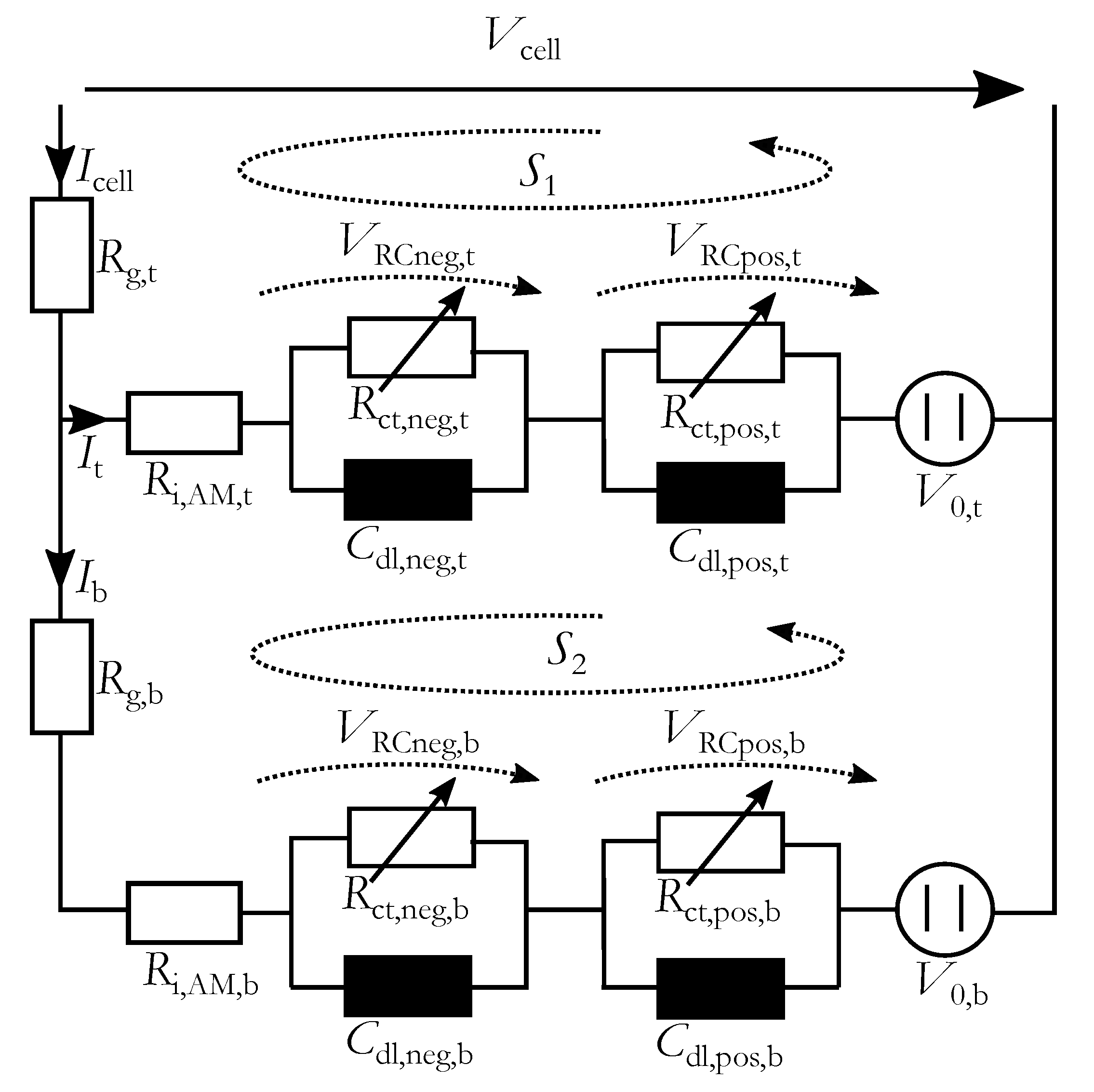
To reproduce the changes of impedance spectrum due to stratification a spatially-resolved equivalent electrical circuit (srEEC) was used. It consists of two layers to simulate inhomogeneous current distribution over the height of the electrodes, which is intensified by the stratification. Every layer contains a resistance connected in series to two RC-elements with the charge-transfer resistances and the double-layer capacitances for negative and positive electrode, respectively. The current dependency of the charge-transfer process in the lead-acid battery is significant in a wide range of charging and discharging currents and is considered here [23]. With the corresponding double-layer capacitance the characteristic form of the impedance spectrum is generated. A voltage source indicates the open-circuit voltage (OCV), which depends on the local acid density. The resulting srEEC is shown in Figure 3.
V 0 , x = ρ x + 0.84 V
The relationship between OCV and the density ρ x is assumed to be linear (see Equation (2)), which is a good approximation for a wide range of the acid density [8].
The ohmic resistance of a lead-acid battery comprises of the lead grid resistance, the active mass and the electrolyte resistance as well as the resistances of the intersections from grid to active mass and to the electrolyte. Here the grid resistance is considered separately and is named R g , t for the top part and R g , b for the bottom part. The other components of the ohmic resistance are summarized in the resistances R i , A M , t and R i , A M , b .
The charge-transfer resistances of the negative R c t , n e g and positive R c t , p o s electrodes were connected in parallel to the corresponding double-layer capacitances ( C d l , n e g and C d l , p o s ). On the negative electrode a second electro-chemical process is present, which can be modeled with an additional RC-element [23]. However, this process could not be described yet [16] and the share to the total battery impedance is small, so that this second RC-element is not considered here.
The Butler-Volmer equation describes the dependency of the charge-transfer rate I on the potential difference to equilibrium potential of the electrode η and is presented in Equation (3). I 0 is the exchange current, α is the symmetry factor between charging and discharging reaction, n is the number of electrons involved in the reaction, F is the Faraday constant, R is the gas constant and T is the temperature in Kelvin [24]. The Butler-Volmer equation provides the current rate I through the charge-transfer resistance.
I = I 0 · e x p α · n · F R · T · η e x p 1 α · n · F R · T · η
The charge-transfer resistance R c t is the quotient of η and I. When I is measured or determined from a system of equations, which is the case here, Equation (3) needs to be resolved for η . This was done numerically with the Matlab function vpasolve.
Due to the nonlinearity of the Butler-Volmer equation, a distinction between the small-signal and the large-signal value of R c t was made here. The small-signal value R c t , s s is measured during EIS with a small amplitude of sinusoidal current and corresponds to the derivative of the Butler-Volmer equation resolved accordingly to η (see Equation (4)). For the calculation of the current distribution in the srEEC the large-signal value R c t , l s is required (Equation (5)), which is equal to the integration of the Butler-Volmer equation resolved accordingly to η over current I [16].
R c t , s s = δ η I δ I
R c t , l s = η I
Equation (3) could be parameterized for the positive electrode in charging and discharging direction, but for the negative electrode only in discharging direction. In charging direction the low concentration of Pb 2 + -ions, caused by a low dissolution rate of PbSO 4 crystals, limits the charge-transfer process on the negative electrode and induced an increase of the charge-transfer resistance. The dissolution rate is affected by the surface area volume ratio of the crystals and not by any over-potentials [16]. In discharging direction the SO 4 -ions are relevant for the reaction and because of their high concentration the charge-transfer process is not limited. The dissolution rate dependent concentration of Pb 2 + -ions for charging could be modeled and integrated in the Butler-Volmer equation, as it is described by Thele and Sauer [23,25] However, this would make the model complex and computationally intensive, so that the measured SoC and current dependency of R c t , n e g in charging direction was described with a surface polynomial function (Equation (17)).
Because of the inhomogeneous current distribution the SoC levels in the top and the bottom become differently, so that the SoC-dependency of the single elements are included in the model. The dependency on SoC is induced by the changing conductivity and density of the acid, the reduction of porosity and the augmented accumulation of lead-sulfate cystals on the surface of the electrodes towards low SoC.
The exchange current I 0 includes the activity of the SO 4 -ions in the electrolyte as factor. For the activity the molar concentration of the electrolyte is used approximately [24]. During the test procedure with stratified electrolyte the molar concentration varied between 4.24 mol L−1 and 6.25 mol L−1, so that due to the concentration change I 0 increased by 47% from low to high concentration. In the parameterization measurements the acid concentration increased only by 6% from 4.681 mol L−1 at 0% SoC to 4.972 mol L−1 at 90% SoC. The small concentration change over SoC during parameterization is caused by the large volume of the electrolyte ( 1200 mL) in the test cell. Because of this small concentration change the dependency of I 0 on molar concentration was separated from the measured SoC dependency. The change of the exchange current over the concentration or the SoC was assumed to be linear, as the OCV SoC relationship was modeled as linear as well (see Equation (2)). This linear change of I 0 was subtracted from the measured I 0 values over SoC. The modified SoC dependency describes now the change of I 0 caused only by transformations in the active mass and is given in Section 2.4. The concentration dependency is modeled using Equation (6) with the present molar concentration c and I 0 , r e f , the exchange current at present SoC and at c r e f , the molar concentration at 0% SoC.
I 0 = I 0 , r e f ( c = c r e f ) · 1 + ( c c r e f c r e f
Equation (6) is applied on I 0 of the positive and the negative electrode in discharging direction. For R c t , n e g in charging direction this separation of the concentration dependency was not made, as the measured increase of the charge-transfer resistance in charging direction is significantly higher than changes generated by the acid concentration.
For the resistances R i , A M , t and R i , A M , b a separated acid concentration dependency had to be introduced as well. During parameterization measurements the conductivity of the acid in the test cell increased from low to high SoC [8]. However, the parameterization measurements presented a decrease of the conductivity (see Section 2.4). With 20% the decrease is lower than measured by Thele on lead-acid starter-batteries (37% for 20 °C) [23]. So the decrease of acid concentration in the test cell extenuated the ohmic resistance increase towards low SoC and the increase is mainly generated by the accumulation of lead-sulfate crystals and the change of porosity. Therefore, a separate consideration of the concentration dependency of R i , A M was implemented. The rate of the electrolyte resistance on R i , A M could not be measured separately, but it was assumed that the electrolyte resistance provides the main part in R i , A M . Equation (7) describes this dependency with R i , A M , h o m o g e n e o u s as the resistance corresponding to the present SoC and determined with Equation (20), d r i , a m as the relative change of specific resistance per g/cm 3 density change (here 3 (g cm−3)−1, based on data from Berndt [8]), ρ r e f as reference density (here 1.28 g cm−3) and ρ x as the present densities in the top and bottom of the cell.
R i , A M = R i , A M , h o m o g e n e o u s ( S o C ) · ( 1 + d r i , a m · ( ρ r e f ρ x ) )
In case of stratification this equation is used to adapt R i , A M in the top and the bottom of srEEC to the local acid densities. The influence of these separations of the acid concentration dependence from the measured SoC dependency is presented in Figure S1 provided as supplementary material.
The SoC-dependency of the double-layer capacitances are described with simple polynomial functions (provided in Section 2.4) and no separation of the acid concentration dependency was considered, as the capacitances does not influence the current distribution in the steady-state.
The simulation using this srEEC starts with the calculation of initial values for R i , A M , x and C d l , x based on initial local SoC. The capacitances are not charged at the beginning, therefore they can be assumed as short circuit and the voltages V R C , x is equal to zero. The current I t 0 is determined with Equation (8) and I b 0 is determined with Equation (12). The current I c e l l is the set DC-current during EIS.
I t 0 = I c e l l R g , b + R i , A M , b + V 0 , b V 0 , t R g , b + R i , A M , b + R i , A M , t
In the next step the R c t , x values are determined using the Butler-Volmer equation or Equation (17) for charging currents with I as the currents, which flow through the resistances. At the beginning these currents are zero.
With Equation (9) the voltage drops V R C , x over the RC-elements are calculated for every RC-element. The parameter n is the counter for the time steps, while n x specifies the values from previous time steps. For I x n 1 and I x n 2 the same value are used at first, which are the initial values for I t and I b .
V R C , x n = V R C , x n 1 · 2 · R c t , x · C d l , x Δ t 1 + R c t , x · I x n 1 + I x n 2 2 · R c t , x · C d l , x Δ t + 1
With the determined V R C , x the cell voltage V c e l l is calculated with Equation (10), which was generated with the Kirchhoff’s voltage law applied to the closed circuit S 1 in Figure 3.
V c e l l n = I c e l l · R g , t + I t n 1 · R i , A M , t n + V R C , n e g , t n + V R C , p o s , t n + V 0 , t n
At this point all values in the srEEC are calculated for one simulation step. At next, the local currents I t n and I b n are determined for next simulation step using the perviously calculated voltages V R C , x (Equations (11) and (12)).
I t n = I b a t t · R g , t + R i , A M , t n + V R C , n e g , b n + V R C , p o s , b n + V 0 , b n V R C , n e g , t n V R C , p o s , t n V 0 , t n R i , A M , t n + R g , b + R i , A M , b n
I b n = I b a t t I t n
With these new values the new local S o C x n are determined as well (Equation (13)). Here to an half of C n o m is used for SoC, as the local SoC corresponds to an half of the electrode, respectively.
S o C x n = S o C x n 1 + Δ t · I x n 3600 s · 100 % 0.5 · C n o m
The duration of one time step Δ t is adapted to the dynamic change of the currents through the capacitances. Therefore these currents are determined with Equation (14) for the present simulation step and are compared with the values from previous step.
I C d l , x n = I x n 1 V R C , x n 1 R c t , x
The duration Δ t is used to calculate V R C , x . If the changes of the currents between two steps are too big, Equation (9) is not valid anymore and the model becomes instable. The current changes are limited to 0.02 A. If the limit was exceeded, Δ t is divided by 10 and the values for V R C , x are calculated again for the same simulation step, until the differences are below the limit or Δ t is equal 1 × 10 −5 s. A duration of 1 × 10 −5 s for Δ t ensures the stability of the model with the used parameters and the adaption of Δ t reduces the simulation duration and generated data volume.
The determined currents through the capacitances (Equation (14)) are used in the next simulation step to determine the currents through R c t , x , which are the differences between I x and I C d l , x n 1 .
The model does not simulate the local acid density on the basis of diffusion, generation and consumption of sulfate ions during charging and discharging, gravity and electrolyte mixing, like in the work of Kowal et al. or Sauer [19,25] In the test cell a homogeneous SoC could be set before the measurements with stratification, so that the initial condition of the acid was well known for Strat. X. Furthermore, the duration of EIS measurements, which have to be simulated, was only 14.5 h, so that diffusion processes did not change the local acid densities significantly.
During discharging with constant current the local acid densities are reduced by the consumption of SO 4 2 ions. The generated density gradient between the pores and the bulk forces diffusion, so that an equilibrium state between consumption and diffusion keeps the acid density constant, but lower than the measured value. The same holds for the charging direction. This local density change cannot be measured and is not considered here.
The stratification itself generated equational local currents over the electrodes between top and bottom part, which discharged the bottom part and charged the top part, so that the density difference decreased measurably over time. This is considered in the model with a linear decrease of the density difference over time, parameterized with the measured acid densities before and after the EIS set. During Strat. 1 the acid density changed with 1.72 × 10 −7 g cm−3 s−1 and during Strat. 2 with a higher rate of 3.16 × 10 −7 g cm−3 s−1 because of the larger density difference.
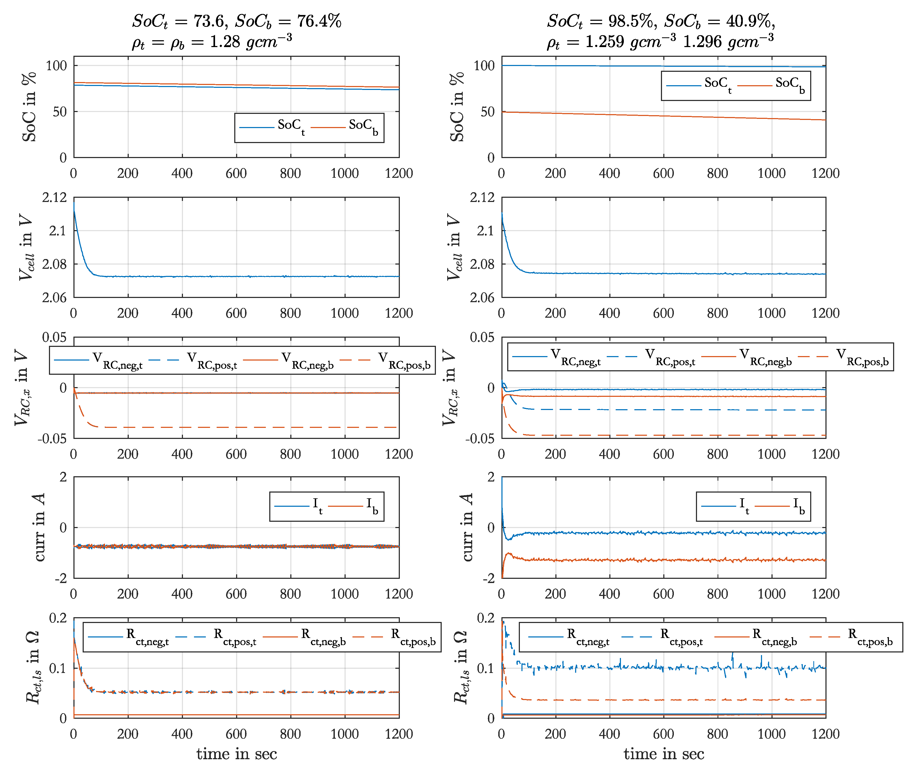
With this model the discharge-charge cycles during an EIS set were simulated. The measured acid densities before the EIS set were used as initial values. The initial local SoC were 80 % for Ref. 1 and Ref. 4. After an EIS set the local SoCs were different and for the subsequent measurements only the acid was either homogenized and stratified and not the local SoC. In these cases the calculated local SoC from the end of the simulated previous measurement were used as initial values for the next simulation.
The output of the simulation is the cell voltage, the local currents, the local SoCs and the values of the srEEC elements over time. Furthermore, one spectrum per discharge or charge phase with constant current is calculated. The impedance of the srEEC is determined at defined times of the simulation with the current srEEC element values using the Kirchhoff’s voltage and current laws. The used equipment for EIS measured the impedances on the test cell at defined frequencies, which can be recalculated to a time, at which the single impedances were determined during EIS measurements with consideration of the three performed sinusoidal waves per frequency. In the simulation the number of frequencies was limited by the maximum SoC change of 4% during EIS as it was the case in the measurements. To generate a shape of the spectra, which is comparable with the measured spectra, the inductance L of the cell ( 1 × 10 7 H) was included and the double-layer capacitances are expected as Constant-Phase-Elements (CPE) in the impedance calculation. The impedance spectrum of a CPE in parallel to a resistance has the shape of a depressed semi-cycle. The depression is defined by the parameter ζ from Equation (23). With Equation (15) the impedance of the double-layer capacitances were calculated in the simulation, using C d l from Equation (22) or the fixed value for positive electrode (see Section 2.4).
Z ̲ C P E = 1 j · ω · C d l ζ

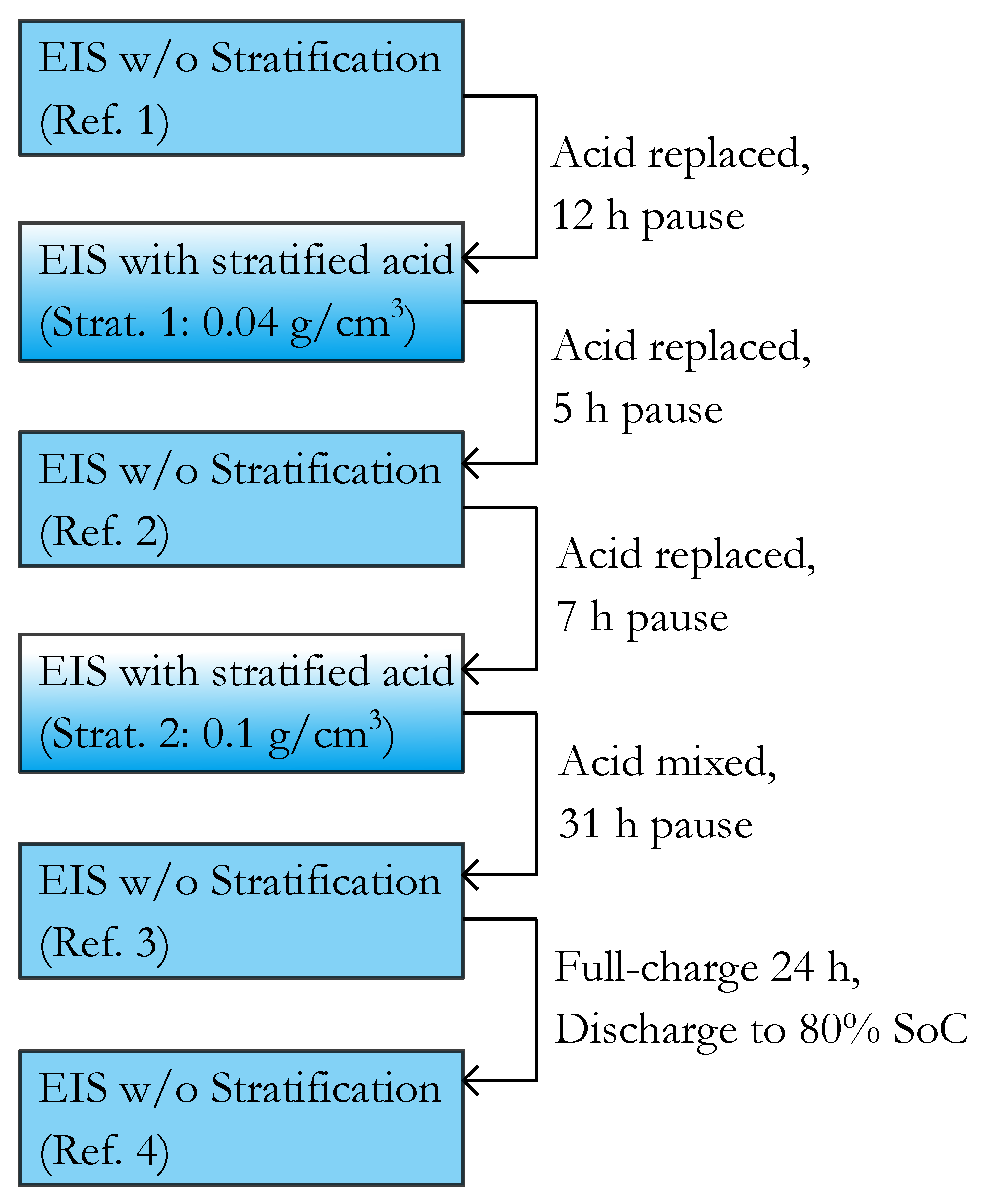
2.4. Parameterization

For the parameterization of the srEEC the same EIS set as denoted in Section 2.1 was performed at 90%, 80%, 60%, 40%, 20%, 10% and 0% SoC. At the beginning the test cell was charged for 24 h with constant-current-constant-voltage charging ( 5 I20, 2.6 V) followed by a pause of 24 h. The single SoC levels were set by discharging with 2 I20 and a subsequent pause of 5 h. During the measurement the acid was mixed to avoid stratification. These parameterization measurements were performed in parallel to the stratification measurements on another test cell with the same configuration.
All impedance spectra of the parameterization measurement were fitted to an equivalent electrical circuit with one resistance connected in series to one RC-element containing the charge-transfer resistance and the double-layer capacitance of the negative electrode. The fitting process is equally performed as described in [17]. The positive electrode parameters were not determined from the spectra, as in most impedance spectra the half-circle of the positive electrode was not adequately visible or affected by time-variant processes.
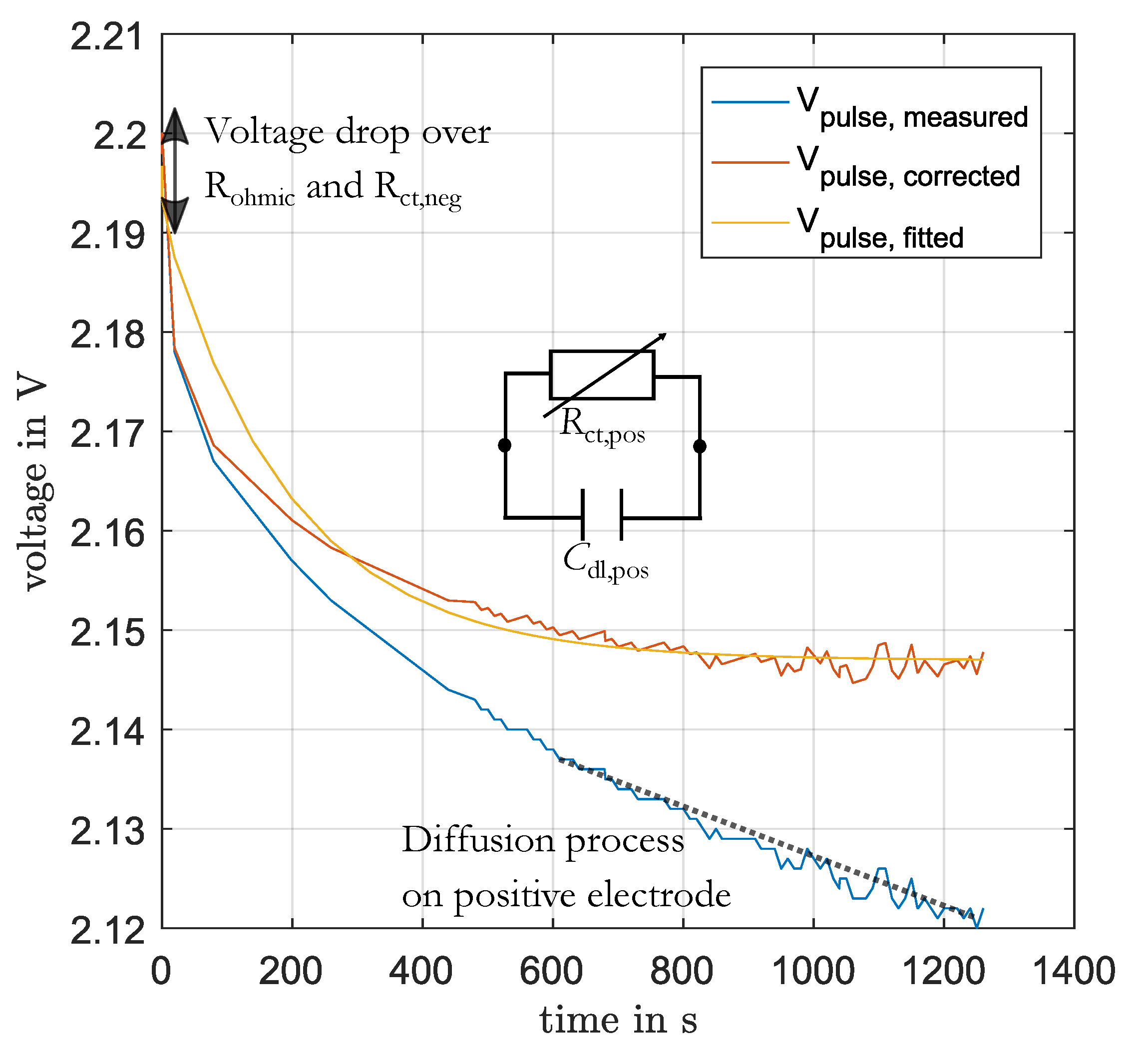
The charge-transfer process and double-layer capacitance of the positive electrode were parameterized from the voltage response during the charging and discharging of 1% SoC before EIS. This voltage response was fitted to an RC-element in time-domain using the function fit in Matlab with default settings. Before, the linear change of voltage (with slope m), generated by diffusion to the end of the pulse, was subtracted as well as the voltage drop over the ohmic resistance R o h m i c and the charge-transfer resistance of the negative electrode R c t , n e g (see Equation (16)). In Figure 4 this process is illustrated. The values for R o h m i c and R c t , n e g were determined for the present DC-current and SoC from the previous parameterization of these elements. The value for the slope m was determined by the fitting of a linear function to the last part of the pulse.
V p u l s e , c o r r e c t e d ( t ) = V p u l s e , m e a s u r e d ( t ) I D C H ( R c t , n e g ( I D C H , S o C ) + R o h m i c ( S o C ) ) m · t
Because of the current dependency of the charge-transfer resistance this approach is not able to determine the double-layer capacitance correctly [3]. The voltage curve is nonlinear and cannot be described by a linear model. However, for the simulation of the current distribution the resistances are relevant and not the capacitances. This also means that the simulated impedance spectra will differ from the measured spectra in the part of positive electrode.
The R c t values at different DC-currents were used to determine I 0 of Equation (3) for the positive and negative electrodes, while α was set fix to 0.25 for the positive electrode and 0.407 for the negative electrode. The values for α were determined from previous parameterization process of Butler-Volmer equation with variable I 0 and α . However, the resulting α values were not constant over the DC-currents, which should be the case. Therefore the average of the single α values were used as fixed value.
I 0 for negative electrode is only valid for discharging, because the measured R c t , n e g in charging direction could not be described by the Butler-Volmer equation, as already described. The measured SoC and current dependency of R c t , n e g in charging direction is described with the surface polynomial function in Equation (17) with the local currents I x and local SoC values S o C x . The R c t values together with the fitting curves are presented in Figure A2.
R c t , n e g , s s = 6.47 × 10 3 Ω + 2.48 × 10 5 Ω % 1 · S o C x + 2.9 × 10 4 Ω A 1 · I x 5.18 × 10 7 Ω % 2 · S o C x 2 1.68 × 10 4 Ω % 1 A 1 · S o C x · I x + 1.15 Ω A 2 · I x 2 + 1.48 × 6 3 Ω % 2 A 1 · S o C x 2 · I x + 1.53 × 10 5 Ω % 1 A 2 · S o C x · I x 2 1.72 × 10 4 Ω A 3 · I x 3
Equation (17) describes the polynomial function for the small-signal value of R c t , n e g . This value was used to calculate the impedance spectrum during simulation. For the calculation of the voltages and current distribution in the srEEC, the large-signal values are required, as already described in Section 2.3. The large-signal value was determined from the integration of Equation (17) from 0 A to the present local currents I t and I b .
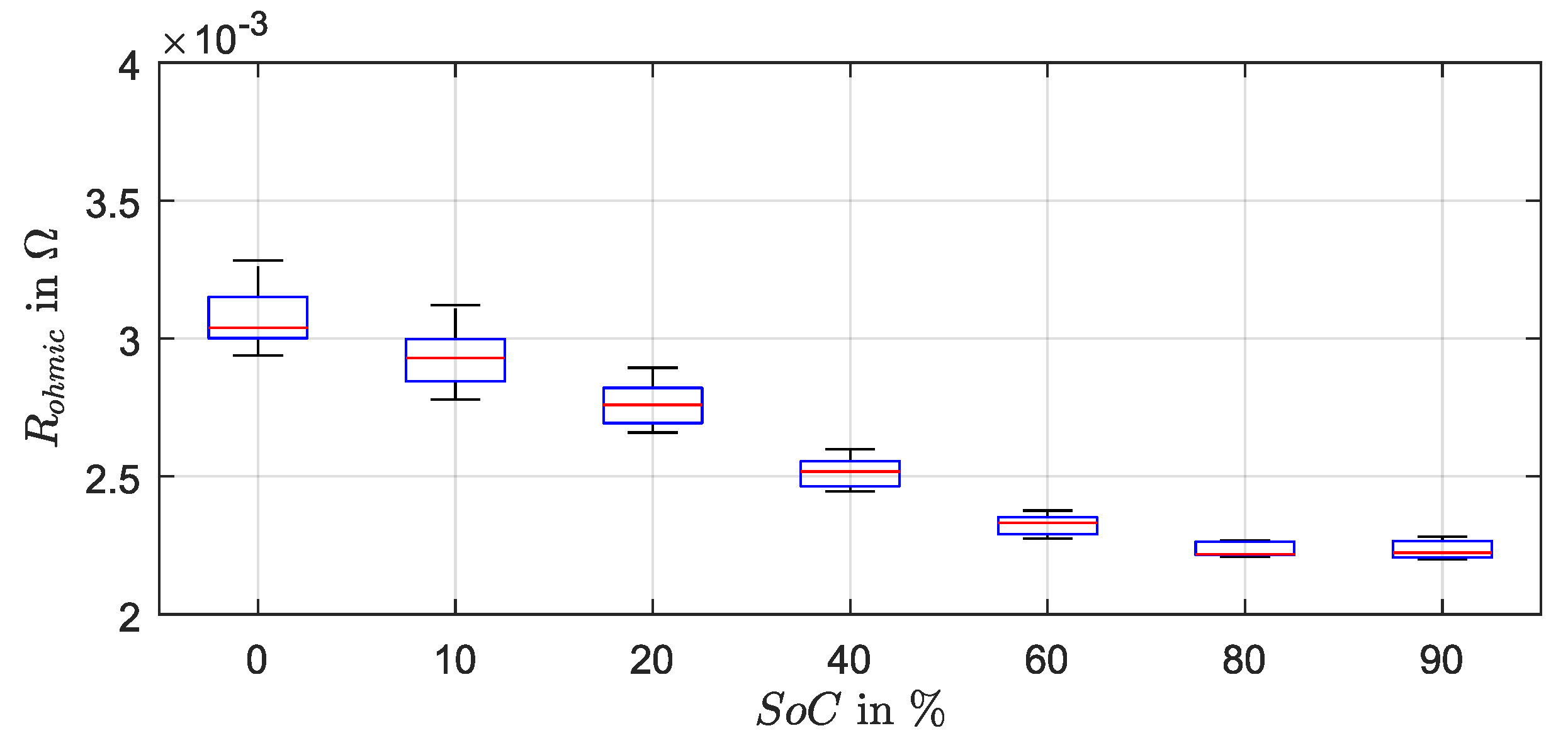
The measured SoC-dependency of the ohmic resistance is described by a polynomial function given in Equation (18). Figure A1 shows the determined resistance values over SoC as boxplot.
R o h m i c = 8.33 × 10 8 Ω % 2 · S o C 2 1.70 × 10 5 Ω % 1 · S o C + 3.06 × 10 3 Ω
The resistance of the lead grid is not SoC-dependent and was separated from the measured ohmic resistance, like presented in the srEEC with R g , t / b and R i , A M . From the design of the lead grid the grid resistance on the top and the bottom was estimated. The grid was 14.5 cm wide, 11 cm high and 1.85 mm thick. The grid bars were 2 mm wide in the middle part and 1 mm in the border area. With 11 bars of 2 mm and 8 bars of 1 mm and a specific resistance of lead of 0.208 Ω mm2/m a resistance value of 0.187 m Ω was calculated for the top part ( R g , t ). For the bottom part with 2 bars of 2 mm and 13 bars of 1 mm the grid resistance R g , b amounted to 0.33 m Ω .
The SoC-dependency of the measured ohmic resistance was attributed to R i , A M . To parameterize this dependency of R i , A M Equation (19) was solved with the Matlab function vpasolve. The equation describes the total impedance of the EEC in Figure 3 for high frequencies, when the RC-elements can be assumed as short-circuits.
R o h m i c = 2 · R g , t + ( 2 · R g , b + R i , A M ) · R i , A M 2 · R g , b + 2 · R i , A M
After Equation (19) was solved for various values of SoC, the determined values for R i , A M over SoC were used to parameterize the polynomial function of R i , A M given in Equation (20).
R i , A M , h o m o g e n e o u s = 1.66 × 10 7 Ω % 2 · S o C 2 3.39 × 10 5 Ω % 1 · S o C + 5.07 × 10 3 Ω
The SoC dependency of R c t , n e g in charging direction is covered by Equation (17). For discharging the determined I 0 , n e g of R c t , n e g over SoC can be described with a polynomial function (Equation (21)).
I 0 , n e g = 3.35 × 10 4 A % 2 · S o C 2 + 4.71 × 10 2 A % 1 c f u l l c r e f c r e f · 100 % · S o C + 1.77 A
According to the separation of acid concentration dependency of I 0 , described in Section 2.3, the parameterized factor of the second term in Equation (21) is adapted. c f u l l is the molar concentration at 100% SoC ( 4.972 mol/L) and c r e f equals to the molar concentration at 0% SoC ( 4.681 mol/L).
I 0 , p o s of the positive electrode did not change significantly over SoC (see Figure A2), so that an average value of 0.15 A was used over the whole SoC range.
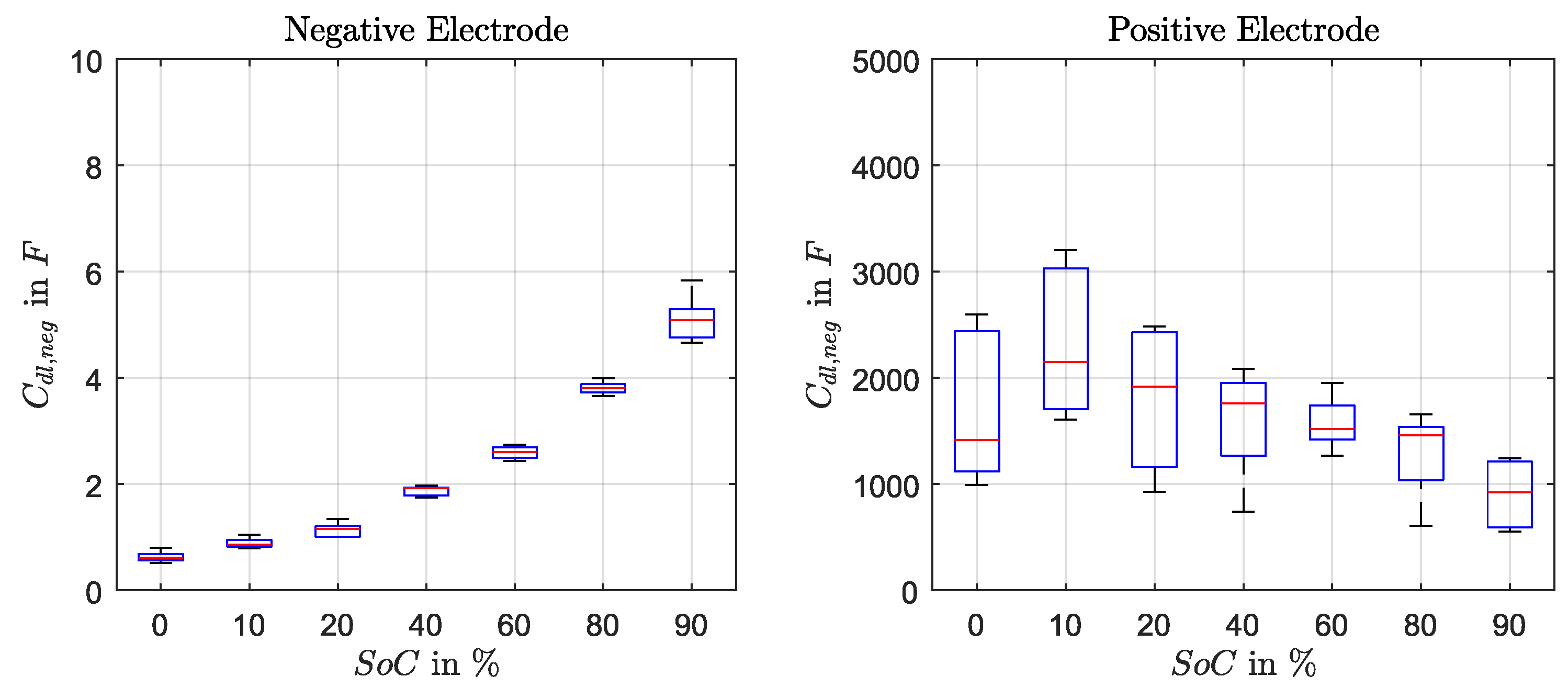
The double-layer capacitance of negative electrode C d l , n e g decreased with the SoC and is described as polynomial function (Equation (22)). For C d l , p o s of the positive electrode a fix value of 1500 F was used, although an increase of the capacity towards low SoC was observed. However, due to the fact that the determination method using discharge pulses in time-domain is not accurate enough this SoC-dependency was not implemented. Figure A3 presents the capacitance values as box plots.
C d l , n e g = 4.01 × 10 4 F % 2 + 9.89 × 10 3 F % 1 + 7.12 × 10 1 F
To generate a comparable shape of the simulated impedance spectra, the double-layer capacitances were used as CPE with the parameter ζ (Equation (15)). The SoC-dependency of ζ was also determined from the parameterization measurements are is given in Equation (23).
ζ = 0.59 + 2.95 × 10 2 A 1 · I x + 1.05 × 10 3 % 1 · S o C x
The parameters of R i , A M , h o m o g e n e o u s are already adapted to the srEEC. The determined capacitance value using Equation (22) and the fix value of C d l , p o s are valid for a one-layer-EEC. In the srEEC, however, one capacitance corresponds to the half of an electrode. Therefore the determined values have to be divided by two.
The exchange currents I 0 are surface area dependent, so that the values are divided by two as well for the srEEC. R c t , n e g for charging direction is multiplied with 2 to be adapted for the srEEC, based on the general dependency of ohmic resistance on the surface area, which is an approximation for the charge-transfer resistance.
Impedance spectra were generated with an 1D-model and the srEEC using the determined parameters with the described adaption for the srEEC. These spectra, presented in the supplementary material, show no differences.

3. Results

3.1. Measurements on Test Cell

Before the impedance spectra, performed during Ref. X and Strat. X, were fitted, the single values of the spectra were checked with the zHit method [21]. In all spectra with superimposed discharging DC-currents the impedance values passed the zHit check, which correspond to the high-frequency tail and the first semi-circle. These spectra could be used for fitting without any restrictions.
The spectra with superimposed charging DC-currents had less valid impedance values. None of the spectra with + 4.5 I 20 , + 6 I 20 and + 8 I 20 had enough valid data points in the first semi-circle. With progressing test procedure more and more spectra with superimposed charging DC-currents became useless for fitting. In Figure 5 impedance spectra with superimposed DC-currents of + 1 I 20 , + 3 I 20 and 8 I 20 are presented, recorded during the test procedure. The squares mark the impedance values, which passed the check with the zHit method.
While during Ref. 1 all of the presented spectra have enough valid points for fitting, the number of valid points decreased with the following EIS sets. The + 3 I 20 spectra in Ref. 3 and Strat. 2 had almost no valid points. After the full-charge of the test cell (Ref. 4) the validity of the spectra improved and is comparable with the validity of the spectra performed in Ref. 1. The 8 I 20 spectra are presented here for comparison and as example for all spectra with superimposed discharge currents, as these spectra provided always an adequate number of valid data points during the whole test procedure.
In the following the fitting results are presented. Figure 6 shows the EEC element values together with the residual from fitting of the spectra from EIS sets Ref. 1, Strat. 1, Ref. 2 and Ref. 4. The EIS set Ref. 4 was performed after 24 h full-charge of the test cell and are presented in the figure for a direct comparison with Ref. 1. In Figure 7 the fitting results from Ref. 2, Strat. 2, Ref. 3 and 4 are shown. Only the results are presented, which come from the impedance spectra with sufficiently enough data points for fitting. For the ± 4.5 I 20 spectra two data points per EIS set are presented in the figures, as these EIS were performed at the beginning and at the end of the EIS set. Values for R o h m i c , R c t , n e g and A d l , n e g determined from the last ± 4.5 I 20 spectra are all larger than from the first ± 4.5 I 20 spectra.
The inductance L, which is generated by the connections of the test cell, varied by 10 % between the EIS sets. This comes from unplugging the measurement equipment and demounting the housing cover during the test procedure. This is not an effect of stratification. The residual for all EIS sets is low with 0.4 × 10 4 Ohm on average, which indicates successful fittings.
Almost all values of R o h m i c during Strat. 1 are smaller by 0.03 m Ω than during the reference measurements presented in Figure 7. R o h m i c varies between the reference measurements by 0.03 m Ω . Furthermore, a light current dependency of the ohmic resistance is visible. The resistance values increase by 6% from large to small discharging currents.
The charge-transfer resistance R c t , n e g as well as the double-layer capacitance A d l , n e g in Figure 6 and Figure 7 increase continuously from Ref. 1 to Ref. 3. The increasing rate from one EIS set to the next EIS set of R c t , n e g is larger towards charging DC-currents. The values corresponding to Ref. 4 decreased again. Over the superimposed current rates R c t , n e g describes the well known current-dependency.
The parameter ζ in Figure 6 is not significantly affected neither by the stratification of the acid nor by the following reference measurements. A current dependency of ζ for discharging currents is visible for all EIS sets in Figure 6 and Figure 7.
In Figure 7 the values from Strat. 2 are only presented for discharging DC-currents, as the other spectra had not enough valid data points for fitting. Similar to Strat. 1 the values for R o h m i c from Strat. 2 are decreased in comparison to the reference measurements in this figure. Only for 6 I 20 and 4.5 I 20 measured at the end of the EIS set R o h m i c is higher in Strat. 2 than in the references.
Similar to Figure 6 R c t , n e g increases with every EIS set in Figure 7, except for Ref. 4, where the resistance drops to the lowest values presented in the figure. Another difference is, that the largest values for R c t , n e g were measured during the Strat. 2 EIS set with 1 I 20 , 6 I 20 and 4.5 I 20 repetition. These are the last DC-currents measured during the EIS set.
Also A d l , n e g increases with every EIS set except Ref. 4. However, for some DC-currents the largest, measured capacitance was measured during Strat. 2. Furthermore, the increase of capacitance is larger at 8 I 20 and 6 I 20 than at smaller discharging DC-currents.
For the two last performed DC-currents in EIS sets Strat. 2 and Ref. 3 a decrease of ζ is visible in Figure 7. This is the only significant variation of ζ ;

3.2. Simulations with Spatially-Resolved Equivalent Electrical Circuit

With the srEEC introduced in Section 2.3 the performed EIS sets on the test cell were simulated. In Figure 8 the current distribution together with the local SoC, the voltages over the RC-elements, the resistance values for R c t , x as well as the simulated cell voltage V c e l l are shown over time during discharging of 5% SoC with 3 I 20 .
On the left side, the results for homogeneous electrolytes are shown. The local SoCs differ by less than 2% from each other at the end of simulation time. The difference was generated during the previous cycles with ± 4.5 I 20 , ± 1.5 I 20 and ± 8 I 20 . Because of the grid resistance the currents I t and I b differ from each other. In the example in Figure 8 the current difference is 0.1 A (6.7% of 3 I 20 ). This generates the difference between the SoC values. The differences between top and bottom of the voltage drops and of the resistance values are small, too.
On the right side the results of the same discharge pulse are presented, but with stratified electrolyte as it was the case during Strat. 1. The local SoCs have already a difference of almost 60%, differences between local currents and voltages are clearly visible. The top part of srEEC is discharged with only 0.23 A, while the bottom part is discharged with 1.27 A. This difference generates a difference in the charge-transfer resistances and also a huge SoC difference.
While the current rate in the bottom part is larger during discharging, it is smaller during charging, when the electrolyte is stratified. During the simulated reference measurements after stratification (Ref. 2), the current rate in the top part is larger for charging and discharging. Because of the lower SoC in the bottom part and the consequently larger resistance values, this inhomogeneous current distribution arises during simulated Ref. 2.
The corresponding impedance spectra for the discharge pulses in Figure 8 are presented in Figure 9 on the left side. On the right side spectra with + 3 I 20 DC-current are presented.
The spectra with homogeneous electrolyte can be compared with Ref. 1 and the spectra simulated with stratification can be comparable with Strat. 1. The first semi-circle increased with the presence of stratification. The increase is larger for charging DC-current, like in the measurements. The high-frequency tail, which crosses the x-axis, is also increased with stratification, which was not the case in the measurements.
In Figure 10 the fitting results of the simulated spectra during Ref. 1, Strat. 1 and Ref. 2 are presented. For fitting an EEC with only one layer of inductance, ohmic resistance and one RC-element was used like for the fitting of the measured spectra.
The values for R c t , n e g from simulation increased from Ref. 1 to Strat. 1, as in the measurements. Between Strat. 1 and Ref. 2 the charge-transfer resistance does not change.
The capacitance A d l , n e g at stratification is for some currents smaller and for some currents larger than at the reference Ref. 1. For Ref. 2 the capacitance is decreased, which is differently to the measurements. ζ is not affected by stratification as it could be observed in the measurements.
The resistance R o h m i c , is larger at stratification than at Ref. 1 for the DC-currents ± 3 I 20 , ± 1 I 20 and + 8 I 20 , which does not match to the measurements. In the spectra, which are at the beginning of the EIS set, R o h m i c is smaller at stratification, which matches with the measured values as well as the simulated increased values of Ref. 2.
During Strat. 2 R c t , n e g further increased as well as R o h m i c , while A d l , n e g behaved similar like during Strat. 1. In Ref. 3 the same observations can be made as in Ref. 1.
In Figure 11 the local SoC values at the end of every discharge or charge pulse during simulated Ref. 1 and Strat. 1 are presented.
During Ref. 1 a difference of 4.5% between local SoC arises, while during Strat. 1 the difference is significantly bigger at the end with 80%. During simulation the maximum and minimum SoC was limited to 100% and 0%, hence the SoC of the top part did not increase over 100% after the simulation of the + 1.5 I 20 pulse. The generated SoC difference after Strat. 1 did not change anymore during Ref. 2. During Strat. 2 this SoC difference further increased to the SoC limits.

4. Discussion

EIS measurements on a test cell with homogeneous and stratified electrolyte have shown a distinct influence of stratification on the impedance, as it was already observed by Budde-Meiwes et al. [7]. Here the influence was analyzed in more details, as the stratification levels were adjusted and impedance spectra with various superimposed DC-currents were performed.
The results from fitting the measured spectra to an EEC have shown a decreased ohmic resistance during stratification in comparison to the reference measurements before and after. With stratification the ionic conductivity of the electrolyte in the top of the test cell was larger than in the bottom. The resistance for the current was already smaller in the top with homogeneous electrolyte, and with stratification this resistance further decreased. Hence, the ohmic resistance of the cell was reduced with stratified electrolyte.
This assumption based on the simulation results. With the implemented dependency of R i , A M on the electrolyte density this decrease of R o h m i c could be reproduced for the first EIS measurements in the EIS set of Strat. 1. To the end of this simulated EIS set R o h m i c increased above the values simulated with homogeneous electrolyte during Ref. 1. In the simulation a huge difference between the local SoC arose and produced a further increased resistance in the bottom due to the SoC-dependency of R i , A M . This increased resistance dominated the resistance of the cell. It is also an explanation for the larger R o h m i c simulated during Ref. 2. In the measurements only the R o h m i c values measured at the end of Strat. 2 were bigger, than during the reference measurements. Here an improvement of the model is required.
The measured increase of R c t , n e g from Ref. 1 to Strat. 1 could be reproduced with the concentration dependency of the exchange current I 0 in srEEC. Also the increasing difference between Ref. 1 and Strat. 1 towards charging currents could be simulated, but not in the same quantity as observed in the measurements. The continues increase of R c t , n e g in the measurements with every EIS set, except Ref. 4, could not be reproduced in the simulations.
Mattera et al. have determined the sulfation rate in the active mass of electrodes after cycling in stratified electrolyte with the result that the bottom part of the electrodes were sulfated, while the top part was almost free of sulfate crystals [10]. The simulated low SoC in the bottom and 100% SoC in the top after simulating Strat. 1 corresponds to these observations. The accumulated crystals in the bottom generate a higher resistance for the current path and the charge-transfer process, which is considered in the srEEC as well. Over time the accumulated crystals reduce their volume to surface area ratio, as this is energetically more convenient [26]. Because of this grow the dissolution rate of Pb 2 + -ions during charging decreases, so that the charge-transfer resistance in charging direction increased with time. This behavior can be a reason for the measured increase of R c t , n e g and was not simulated in srEEC.
The progressing sulfation during the test procedure can be additionally an explanation for the increased R o h m i c at the end of EIS set Strat. 2. The beneficial effect of the stratification on the conductivity of the electrolyte is rescinded by the increasing sulfation. The decrease of ζ at the end of the test procedure denotes an stronger inhomogeneity in the cell generated by the sulfation, because ζ decreases with increasing inhomogeneity [16].
The measured results of Ref. 4 provide a further confirmation of the previous sulfation process. All resistance values decreased after the full-charge to values similar to them in Ref. 1, because the full-charge dissolved the sulfate crystals and cleared up the surface area for the charge-discharge reaction. The characteristic change of impedance could be also observed during cyclic aging tests [17].
The continues increase of A d l , n e g in the measurements could not be simulated with the srEEC. It was expected that the capacitance decreases with progressing generation of sulfate crystals. This is the reason for the decrease of this EEC element with decreasing SoC (see Figure A3) and this was observed during cyclic aging with sulfation as main aging process [17]. Maybe the form or structure of these sulfate crystals are different, when they grew during stratification. Clarifying chemical determination of sulfation rates after cycling in stratified and homogeneous electrolyte were not performed, yet, so that an explanation for this observation could not be found.
This characteristic behavior of the capacitance together with the decrease of R o h m i c and increase of R c t , n e g can be an indicator for stratification and the consequent aging to be detected online. However, impedances, determined for the online estimation of SoC and State-of-Health (SoH), have to be used with care, if the presence of stratification is possible but not detected by the diagnostic tool in an application.

5. Conclusions

Performed impedance spectra on lead-acid test cells with stratified electrolyte have shown characteristic changes of the ohmic resistance, the charge-transfer resistance and the double-layer capacitance of negative electrode. The resistances changed initially because of the stratification of electrolyte itself, as the electrolyte conductivity as well as the exchange current of the charge-transfer process depend both on the electrolyte concentration. With cycling the test cell when electrolyte was stratified the generated inhomogeneous sulfation started to increase not only the resistances but also the double-layer-capacitance. These observations could be used for the development of stratification detection algorithms.
The developed spatially-resolved EEC could not reproduce all observed influences of stratification on the impedance of the lead-acid test cell. The large simulated difference in SoC between top and bottom needs to be verified. Furthermore, the EEC has to contain a model of the sulfate crystal grow, which increases the charge-transfer resistance in charging direction. However, explanations for the decreased ohmic resistance and the increased charge-transfer resistance could be found. Only for the observed increase of the double-layer capacitance further investigations are required to find a reason.

Supplementary Materials

The following are available online at https://www.mdpi.com/2076-3417/8/7/1018/s1, Figure S1: Simulated impedance spectra with −4.5 I20 superimposed DC-current are presented with different features of the model, Figure S2: Simulated impedance spectra with −4.5 I20 superimposed DC-current at 80% using an 1D and the spatial-resolved model with the same set of parameters, only that the parameters were adapted to spatial-resolved model. Also the measured impedance spectrum for the same DC-current and SoC is shown as well.

Author Contributions

M.K., M.H., C.Z. and D.U.S. conceived and designed the experiments. J.B. acquired the funding and was the project administrator. M.K., C.Z., K.K. and Q.Y. performed the experiments. M.K. and C.Z. analyzed the data. M.K. wrote the paper.

Funding

This research was funded by the European EFRE program grant number EU-1-1-081.

Acknowledgments

The underlying work was conducted within the project BSMS (EU-1-1-081) funded through the European EFRE program. Funds were received from the same program for covering the costs to publish in open access.

Conflicts of Interest

The authors declare no conflict of interest. The founding sponsors had no role in the design of the study; in the collection, analyses, or interpretation of data; in the writing of the manuscript; or in the decision to publish the results.

Abbreviations

The following abbreviations are used in this manuscript:
EISElectro-chemical Impedance Spectroscopy
SoCState-of-Charge
EECEquivalent Electrical Circuit
CPEConstant-Phase Element
srEECspatially-resolved equivalent electrical circuit
OCVOpen Circuit Voltage

Appendix A. Parameterization Results

Figure A1. Determined ohmic resistance values from fitting of impedance spectra measured with discharging DC-currents over SoC.
Applsci 08 01018 g0a1
Figure A2. Determined charge-transfer resistances from fitting of impedance spectra for negative electrode and from pulses for positive electrode, together with the fitting curves of Butler-Volmer equation.
Applsci 08 01018 g0a2
Figure A3. Determined double-layer capacity values from fitting of impedance spectra measured with discharging DC-currents (negative electrode) and from fitting of discharge pulses (positive electrode) over SoC.
Applsci 08 01018 g0a3

References

  1. Karden, E.; Buller, S.; Doncker, R.W. A method for measurement and interpretation of impedance spectra for industrial batteries. J. Power Sources 2000, 85, 72–78. [Google Scholar] [CrossRef]
  2. Huet, F.; Nogueira, R.P.; Lailler, P.; Torcheux, L. Investigation of the high-frequency resistance of a lead-acid battery. J. Power Sources 2006, 158, 1012–1018. [Google Scholar] [CrossRef]
  3. Kiel, M. Impedanzspektroskopie an Batterien unter besonderer Berücksichtigung von Batteriesensoren für den Feldeinsatz. In Aachener Beiträge des ISEA; Chapter Impedanzmessungen an Batterien als Beispiel für Nicht-LTI Systeme; Shaker: Aachen, Germany, 2013; Volume Bd. 67. [Google Scholar]
  4. Huang, W.; Qahouq, J.A. An Online Battery Impedance Measurement Method Using DC–DC Power Converter Control. IEEE Trans. Ind. Electron. 2014, 61, 5987–5995. [Google Scholar] [CrossRef]
  5. Nguyen, T.-T.; Tran, V.-L.; Choi, W. Development of the intelligent charger with battery State-Of-Health estimation using online impedance spectroscopy. In Proceedings of the 2014 IEEE 23rd International Symposium on Industrial Electronics (ISIE), Istanbul, Turkey, 1–4 June 2014; IEEE: Piscataway, NJ, USA, 2014; pp. 454–458. [Google Scholar] [CrossRef]
  6. Osaka, T.; Mukoyama, D.; Nara, H. Review—Development of Diagnostic Process for Commercially Available Batteries, Especially Lithium Ion Battery, by Electrochemical Impedance Spectroscopy. J. Electrochem. Soc. 2015, 162, A2529–A2537. [Google Scholar] [CrossRef]
  7. Budde-Meiwes, H.; Kowal, J.; Sauer, D.U.; Karden, E. Influence of measurement procedure on quality of impedance spectra on lead–acid batteries. J. Power Sources 2011, 196, 10415–10423. [Google Scholar] [CrossRef]
  8. Berndt, D. Maintenance-free batteries: Based on aqueous electrolyte lead-acid, nickel/cadmium, nickel/metal hydride: A handbook of battery technology. In Electronic & Electrical Engineering Research Studies; Chapter the Lead-Acid Battery System; Research Studies Press: Baldock, UK, 2003; Volume 5. [Google Scholar]
  9. Guo, Y.; Yan, W.; Hu, J. Effects of Electrolyte Stratification on Performances of Flood Lead-Acid Batteries. J. Electrochem. Soc. 2007, 154, A1–A6. [Google Scholar] [CrossRef]
  10. Mattera, F.; Desmettre, D.; Martin, J.L.; Malbranche, P. Characterisation of photovoltaic batteries using radio element detection: The influence and consequences of the electrolyte stratification. J. Power Sources 2003, 113, 400–407. [Google Scholar] [CrossRef]
  11. Ruetschi, P. Aging mechanisms and service life of lead–acid batteries. J. Power Sources 2004, 127, 33–44. [Google Scholar] [CrossRef]
  12. Albers, J.; Meissner, E.; Shirazi, S. Lead-acid batteries in micro-hybrid vehicles. J. Power Sources 2011, 196, 3993–4002. [Google Scholar] [CrossRef]
  13. Sauer, D.U.; Garche, J. Optimum battery design for applications in photovoltaic systems—Theoretical considerations. J. Power Sources 2001, 95, 130–134. [Google Scholar] [CrossRef]
  14. Ebner, E.; Burow, D.; Börger, A.; Wark, M.; Atanassova, P.; Valenciano, J. Carbon blacks for the extension of the cycle life in flooded lead acid batteries for micro-hybrid applications. J. Power Sources 2013, 239, 483–489. [Google Scholar] [CrossRef]
  15. Swogger, S.W.; Everill, P.; Dubey, D.P.; Sugumaran, N. Discrete carbon nanotubes increase lead acid battery charge acceptance and performance. J. Power Sources 2014, 261, 55–63. [Google Scholar] [CrossRef]
  16. Kowal, J. Spatially-Resolved Impedance of Nonlinear Inhomogeneous Devices: [Using the Example of Lead-Acid Batteries]; Shaker: Aachen, Germany, 2010; Volume Bd. 53. [Google Scholar]
  17. Kwiecien, M.; Badeda, J.; Huck, M.; Komut, K.; Duman, D.; Sauer, D. Determination of SoH of Lead-Acid Batteries by Electrochemical Impedance Spectroscopy. Appl. Sci. 2018, 8, 873. [Google Scholar] [CrossRef]
  18. Kwiecien, M.; Huck, M.; Badeda, J.; Sauer, D.U. Correct processing of impedance spectra for lead-acid batteries to parameterize the charge-transfer process. J. Appl. Electrochem. 2018, 1–16. [Google Scholar] [CrossRef]
  19. Kowal, J.; Schulte, D.; Sauer, D.U.; Karden, E. Simulation of the current distribution in lead-acid batteries to investigate the dynamic charge acceptance in flooded SLI batteries. J. Power Sources 2009, 191, 42–50. [Google Scholar] [CrossRef]
  20. Schulte, D.; Sanders, T.; Waag, W.; Kowal, J.; Sauer, D.U.; Karden, E. Automatic device for continuous measurement of potential distribution and acid stratification in flooded lead-acid batteries. J. Power Sources 2013, 221, 114–121. [Google Scholar] [CrossRef]
  21. Schiller, C.A.; Richter, F.; Gülzow, E.; Wagner, N. Validation and evaluation of electrochemical impedance spectra of systems with states that change with time. Phys. Chem. Chem. Phys. 2001, 3, 374–378. [Google Scholar] [CrossRef]
  22. Witzenhausen, H. FittingGUI. 2016. Available online: https://github.com/HWitz/FittingGUI (accessed on 22 June 2018).
  23. Thele, M. A contribution to the modelling of the charge acceptance of lead-acid batteries: Using frequency and time domain based concepts. In Aachener Beiträge des ISEA; Chapter Equivalent Electrical Circuit; Shaker: Aachen, Germany, 2008; Volume 50. [Google Scholar]
  24. Newman, J.S.; Thomas-Alyea, K.E. Electrochemical Systems, 3rd ed.; Wiley: Hoboken, NJ, USA, 2004. [Google Scholar]
  25. Sauer, D.U. Optimierung des Einsatzes von Blei-Säure-Akkumulatoren in Photovoltaik-Hybrid-Systemen unter Spezieller Berücksichtigung der Batteriealterung. Ph.D. Thesis, der Universität Ulm, Ulm, Germany, 2003. [Google Scholar]
  26. Kappus, W. Homogeneous nucleation, growth and recrystallization of discharge products on electrodes. Electrochim. Acta 1983, 28, 1529–1537. [Google Scholar] [CrossRef]
Figure 1. The voltage and current profiles of the EIS set containing different superimposed DC-currents in charging and discharging direction.
Applsci 08 01018 g001
Figure 2. The sequence of EIS sets performed with homogeneous and stratified acid. The density values specify the measured acid concenctration difference between top and bottom.
Applsci 08 01018 g002
Figure 3. Spatially-resolved equivalent electrical circuit (srEEC) with two layers to simulate an inhomogeneous current distribution.
Applsci 08 01018 g003
Figure 4. Illustration of the pre-processing and fitting of a discharge pulse for the parameterization of positive electrode.
Applsci 08 01018 g004
Figure 5. Impedance spectra with superimposed DC-currents of + 1 I 20 , + 3 I 20 and 8 I 20 performed during the reference measurements and measurements with stratified acid presented as Nyquist-diagrams. The squares in the diagrams mark the impedance values, which passed the zHit check.
Applsci 08 01018 g005
Figure 6. EEC element values together with the residual from fitting of the impedance spectra in EIS sets Ref. 1, Strat. 1, Ref. 2 and Ref. 4. Positive currents are charging currents and negative currents denote the discharging currents.
Applsci 08 01018 g006
Figure 7. EEC element values together with the residual from fitting of the impedance spectra in EIS sets Ref. 2, Strat. 2, Ref. 3 and Ref. 4.
Applsci 08 01018 g007
Figure 8. Simulated current distribution in the srEEC during discharging with 3 I20. S o C x , V c e l l , V R C , x , I x and the values for R c t , x are shown. On the left side the results from simulation with homogenous acid are presented, on the right side with stratification as during Strat. 1.
Applsci 08 01018 g008
Figure 9. Simulated impedance spectra of the srEEC with ± 3 I 20 for I c e l l . The blue spectra corresponds to simulations with homogeneous electrolyte and the red spectra to simulations with stratified electrolyte as during Strat. 1.
Applsci 08 01018 g009
Figure 10. Fitting results of the simulated spectra during Ref. 1, Strat. 1 and Ref. 2 using an EEC with one layer.
Applsci 08 01018 g010
Figure 11. SoC values of top and bottom part from the end of the simulated discharging and charging pulses. The SoC values are plotted over the chronological order of superimposed DC-currents.
Applsci 08 01018 g011
Table 1. Amount of acid with different densities to generate Strat. 1 and Strat. 2.
DensityVolumeAmount of Substance
homo. acid Ref. 1 1.284 g cm-31160 cm3 5.72 mol
low conc. acid Strat. 1 1.246 g cm-3600 cm3 2.56 mol
high conc. acid Strat. 1 1.308 g cm-3580 cm3 3.19 mol
homo. acid Ref. 2 1.284 g cm-31150 cm3 5.67 mol
low conc. acid Strat. 2 1.20 g cm-3605 cm3 1.48 mol
high conc. acid Strat. 2 1.36 g cm-3630 cm3 4.08 mol
Table 2. Measured acid densities in the top and bottom of the test cell at different states of measurement procedure.
PositionRef. 1Before Strat. 1After Strat. 1Ref. 2Before Strat. 2After Strat. 2Ref. 3
top 1.283 g cm-3 1.256 g cm-3 1.264 g cm-3 1.283 g cm-3 1.239 g cm-3 1.246 g cm-3 1.276 g cm-3
bottom 1.284 g cm-3 1.299 g cm-3 1.289 g cm-3 1.284 g cm-3 1.346 g cm-3 1.320 g cm-3 1.276 g cm-3
difference 0.001 g cm-3 0.043 g cm-3 0.025 g cm-3 0.001 g cm-3 0.107 g cm-3 0.074 g cm-3 0.000 g cm-3

