Article

Comparative Analysis of Current Control Techniques to Support Virtual Inertia Applications †

1
Department of Electrical Engineering and Computer Science, South Dakota State University, Brookings, SD 57007, USA
2
Primus Power, Hayward, CA 94545, USA
3
Schweitzer Engineering Laboratories, Pullman, WA 99163, USA
4
Department of Electrical Engineering, Tribhuvan University, Kathmandu 44600, Nepal
*
Author to whom correspondence should be addressed.
This paper is an extended version of our paper published in IEEE 6th International Conference on Power Systems (ICPS), New Delhi, India, 4–6 March 2016.
Appl. Sci. 2018, 8(12), 2695; https://doi.org/10.3390/app8122695
Submission received: 15 November 2018 / Revised: 7 December 2018 / Accepted: 13 December 2018 / Published: 19 December 2018
(This article belongs to the Section Energy Science and Technology)

Abstract

:
The rapid transition towards an inverter-dominated power system has reduced the inertial response capability of modern power systems. As a solution, inverters are equipped with control strategies, which can emulate inertia by exchanging power with the grid based on frequency changes. This paper discusses the various current control techniques for application in these systems, known as virtual inertia systems. Some classic control techniques like the proportional-integral, the proportional-resonant, and the hysteresis control are presented first, followed by the design and discussion of two more advanced control techniques based on model prediction and machine learning, respectively. MATLAB/Simulink-based simulations are performed, and results are presented to compare these control techniques in terms of harmonic performance, switching frequency, and transient response.

1. Introduction

The global demand for green energy has seen a rapid increase in the past few years due to the decrease in generation costs coupled with a variety of incentives for clean energy production and usage [1]. Consequently, renewable energy sources (RES), such as photovoltaic (PV) and wind energy, constitute a major share of the generation in modern power systems. These RES units have a commonality in terms of unpredictable power output and the fact that they are integrated with the power system through power electronic converters [2]. The traditional power system, which was dominated by large synchronous generators, is now evolving towards an inverter-dominated power system, which decouples the mechanical inertia from the grid [3]. Typically, these RES units are operated as non-dispatchable current sources and provide no inertial response, which leads to dynamic stability issues in the power system. In many cases, this limits the RES penetration levels in the power system [2].
Virtual inertia emulation through appropriate control of power electronic converters has been widely proposed as a possible solution to counteract these issues. Virtual inertia is a combination of control algorithms, energy storage systems (ESS), and power electronics that emulates the inertia of a conventional power system [4]. Inertia can be emulated through use of ESS or by operating the RES units below their maximum power points, providing a reserve for the inertial response [5]. A number of algorithms has been proposed for this in the literature under different names such as virtual synchronous machines [6], virtual synchronous generators [7], synchronverters [8], and synchronous power controllers [9]. In most cases, a “current feedback loop” is employed to inject/absorb the inertial power through these systems. Because this power comes in short bursts based on frequency changes, a well-designed “current feedback loop” with good transient response and low steady-state error is required for a functional implementation.
This paper presents the design and a comparative study of different current control techniques that can be employed for the design of the “current feedback loop”. A comparison of some of the basic current control techniques, including proportional-integral (PI) control, proportional-resonant (PR) control, and hysteresis control was previously presented in [10]. This paper expands on our work in [10] by providing a more in-depth analysis of these techniques along with a discussion on two more advanced control approaches. The advancements in the computational capabilities of modern digital signal processors (DSPs) and field-programmable gate arrays (FPGAs) allows the implementation of these sophisticated control algorithms, which optimize the operation of the “current feedback loop”. Furthermore, the maturity in wide bandgap semiconductor technology means that the power electronics switches can be operated at higher switching frequencies with fewer switching losses [11]. In this regard, the paper incorporates (i) a model predictive control (MPC), which generates optimized switching signals based on a current model [12], and (ii) a method of using an adaptive dynamic programming (ADP) controller to optimize the current control through an online learning-based approach [13,14]. These techniques are compared through MATLAB/Simulink simulations, and conclusions are drawn for the selection of the appropriate current control technique for virtual inertia emulation.
The paper is organized as follows: Section 2 introduces the concept of virtual inertia and describes the basic theoretical aspects of different current control techniques. The design procedure for each of the discussed current control approaches is presented in Section 3. Section 4 analyzes the simulation results and performs a comparative study, and Section 5 presents the conclusions.

2. Virtual Inertia and Current Control Techniques

2.1. Concept of Virtual Inertia

Virtual inertia is a combination of control algorithms, ESS, and power electronics that emulates inertia similar to that of a conventional synchronous generator with a large rotating mass and damper windings. The virtual inertia control algorithm presents RES units and/or ESS as a dispatchable energy source with the capability of responding to frequency changes in the power system. There are numerous methods of implementing virtual inertia that are discussed in the literature. Approaches such as synchronous power controllers discussed in [9] use a complete electromechanical model of a synchronous generator to generate a set of reference voltages. The corresponding current references for the inverter are then generated using the concept of virtual admittance. A current controller is finally used to inject the reference current. Other topologies like the synchronverter [8] and Ise labs topology [15] operate the inverters as voltage sources instead of current sources. A review of these various topologies was discussed in detail in [16,17,18].
A simple implementation of the virtual inertia control algorithm is shown in Figure 1. Since this topology does not implement any electromechanical models within the controller, the implementation is quite straightforward [16,17]. The controller continuously measures the frequency of the system typically using a phase-locked loop (PLL) and generates power references, P V I , based on the change in frequency ( Δ f ) and the rate of change of frequency (ROCOF) ( d ( Δ f ) d t ) as:
P V I = ( K d r o o p Δ f ) + K i n e r t i a d ( Δ f ) d t
where K d r o o p is the damping constant similar to a frequency droop and K i n e r t i a is the inertia constant, which tries to arrest the change in frequency. The calculated reference power is then injected/absorbed to/from the system using a current-controlled voltage source inverter (CC-VSI), which uses a current control loop, which are compared in this paper.

2.2. Proportional-Integral Controller

The current control of grid-connected inverters using PI controllers is a mature control strategy. The design method is fairly simple and straightforward, but has limitations especially in terms of the transient performance. The main distinct advantages are that the switching signals have a constant frequency and the harmonics are well-defined. The PI control method used for virtual inertia emulation uses a nested loop structure with two loops. An outer loop generates the reference power based on Equation (1), and the reference current is then calculated. The faster inner loop is a current control loop used to control the output current of the inverter to this reference value. An inherent drawback of the PI controller is that it cannot track sinusoidal current references, thus exhibiting a steady-state error [19]. To overcome this limitation, a transformation into the direct-quadrature ( d q ) synchronous reference frame is used, which transforms the three-phase a b c currents into constant d q currents, which can be tracked by PI controllers. Furthermore, this allows the application of linear control techniques for the design of the current controller. This approach is classified as synchronous d q frame control in the literature [20].
Figure 2 shows the control structure of a PI Type-2-based current control of the grid-connected inverter along with the benchmark that will be used throughout this paper. The PI Type-2 controller is a variation of the traditional PI controller with an extra pole at the high frequency range to compensate for the high frequency switching noises. A PLL is used to track the phase ω t of the grid voltage [20,21]. The three-phase inverter output current is continuously measured using current sensors and first transformed into the d q domain using the Park transformation ( a b c d q ). The cross-coupling terms ( ω L I d and ω L I q ), which are usually neglected during the design of the PI controller, can also be compensated in the control structure, which improves the dynamics of the controller [20]. Moreover, the grid voltage v a b c is also transformed into the d q domain and fed forward, which helps in stabilizing the output voltage of the inverter faster and also aids in the synchronization process [22]. The output of the PI controllers is then transformed back into the a b c domain using the inverse Park transformation ( d q a b c ) and used as modulating signals for the pulse width modulation (PWM) modulator. The transfer function of the plant (i.e., a grid-connected inverter with an LC filter) for the design of the PI controller can be modeled as [22]:
G p l a n t ( s ) = 1 L s + r L
where r represents the internal resistance of the filter inductor and L is the inductance of the filter inductor. The effect of the capacitance C can also be neglected from the point-of-view of the current control design. A modified form of a PI controller, referred to as a PI Type-2 controller, which includes a high frequency pole in the transfer function compared to a classical PI controller [23], is used in this paper. The transfer function is given by:
C P I ( s ) = K P I 1 + s τ s τ 1 1 + s T p
where K P I is the controller gain, τ is the time constant, and T p is the time constant of an additional high frequency pole introduced to reduce the effects of higher frequency switching noises.

2.3. Proportional-Resonant Controller

The PR controller uses a stationary frame-based current control approach while achieving similar transient and steady-state performance as a PI controller [24]. The implementation of the controller in the synchronous frame means that complex transformations, as in the case of PI controllers, are not required, which is especially beneficial for single-phase systems where PI controllers are difficult to implement [19]. The PR controller shows improved performance in tracking sinusoidal signals compared to PI controllers without the need for the decoupling terms and/or voltage feed-forward terms [25]. A PI controller typically has a high gain at lower frequencies, whereas the PR controller can achieve a high gain around a narrow band near the designed resonant frequency. Because of this high gain, the PR controller is able to track sinusoidal signals around this resonant frequency. The transfer function of a typical PR controller is given by:
C P R ( s ) = K P + K I s s 2 + ω 2
where K P is the proportional gain and K I is the resonant gain. K I defines the width of the frequency band (a high K I resulting in a wider band). This is of special importance while designing PR controllers for virtual inertia systems in weak grids. The frequency of the grid may change significantly, which means a relatively wide frequency band is required for a proper current control scheme. For large frequency deviations, the PR controller may show poor performance [25]. There is another slight variation of the transfer function of the PR controller in [26], but it is known to have poor transient performance, as described in [24].
Figure 3 shows the control structure for the PR controller. Again, the PLL is used to extract the phase information of the grid. The reference d q currents are transformed into a b c signals. It is important to note that the transformation is just used for providing the reference currents in the d q domain, keeping consistency with the other controllers analyzed in this paper. The reference currents could easily be provided in the a b c domain, omitting the need for this transformation. The reference current i a b c * is then compared against the feedback current i a b c , and the error is passed onto the PR controller. The output of the PR controller is finally used as the modulating signal for the PWM modulator.

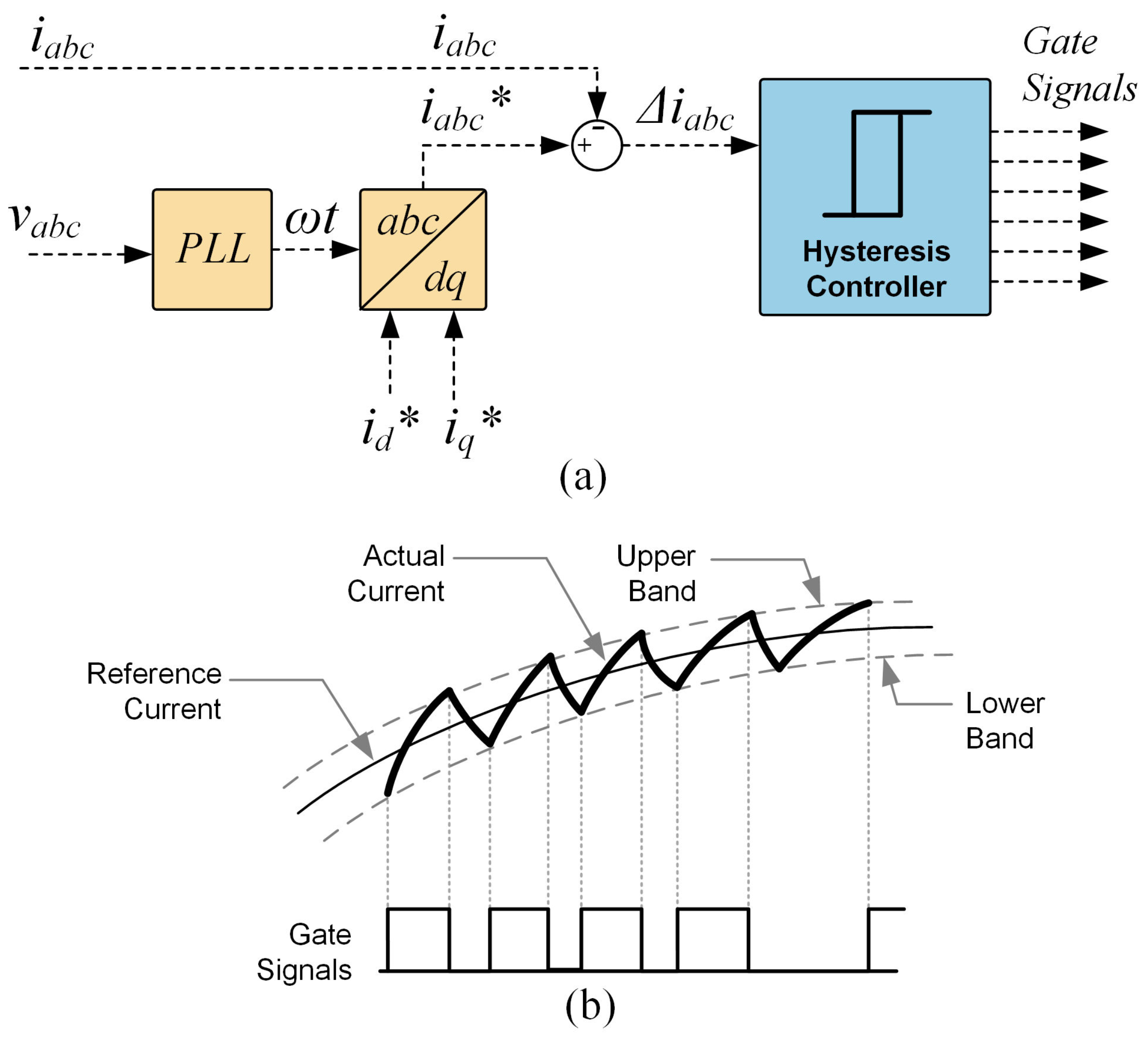
2.4. Hysteresis Controller

The hysteresis current control technique is a simple and effective technique to achieve fast dynamics within the current control loop [27]. The inherent current limiting capability, robustness, and model-free implementation are some of the main benefits of the hysteresis control approach [28]. In this technique, a “hysteresis band” is defined around the reference current that the controller needs to track. The switches of the inverter are then controlled in such a manner that the output current of the inverter always stays within this band; hence, there is no need for a PWM modulator. This greatly improves the transient response time of this control approach, but this also means that the switching frequency is variable, depending largely on the selected hysteresis band and load/operating conditions, making the design of the output filter difficult [29]. Alternate techniques to keep the switching frequency constant are proposed in [30,31]. In [32], a method of using a sinusoidally-varying hysteresis band is proposed to reduce the output current and power ripple. However, for simplicity, a generic hysteresis current controller as shown in Figure 4 is discussed in this paper.
Figure 4a shows the control structure for a hysteresis current controller. The reference current in the d q domain is transformed into the a b c domain. The reference current, i a b c * , is then compared with the feedback current i a b c , and the error is fed into the hysteresis band to generate the switching signals for the three-phase inverter. Figure 4b gives a more detailed description of the gate signals’ generation processes. When the actual current output of the inverter exceeds the pre-defined hysteresis band, the gate signal goes low, causing the current to decay. The rate of decay depends on the time-constant of circuit (r and L parameter values). As the current decays, the current exceeds the lower hysteresis band, and the gate signal goes high, causing the current to rise. In this manner, the actual current waveform is made to follow the reference current within the pre-defined hysteresis band. The hysteresis band selection is often selected to be between 2 and 5% of the reference current [33]. The band is usually limited by the switching capability of the switches and the electromagnetic interference concerns. The lower the band, the higher the switching frequency, and vice versa.

2.5. Model Predictive Controller

MPC is an advanced control technique used to control power electronic systems. The ease in including system non-linearities with an intuitive control design is the main attraction of the MPC technique [34,35]. MPC uses a model of the system to predict the future behavior of the controlled variables. The prediction in turn is used by the controller to generate near-optimal control actions by minimizing a cost function [36].
Figure 5a shows the control structure for current control using MPC. The reference current in the d q domain is transformed into the α β domain. Similarly, the feedback current, i a b c , is also transformed into the α β domain. The MPC controller then uses these signals to generate the gate signals. Figure 5b shows the details of the MPC block. The feedback current is used along with a current prediction model given by Equations (5) and (6) to predict the currents in the next sampling instant [37].
i ^ ( k + 1 ) = 1 r T s + L [ L i ( k ) + T s v ( k + 1 ) T s e ( k + 1 ) ]
where i is the grid current, v is the inverter voltage, and e is the grid voltage. The grid voltage can be estimated as:
e ^ ( k ) = v ( k ) + L T s i ( k 1 ) r T s + L T s i ( k )
An optimization function given by (7) is used within the cost function minimization block that tries to reduce the current tracking error and generates the best switching state [37].
g = | i α * ( k + 1 ) i α ( k + 1 ) | + | i β * ( k + 1 ) i β ( k + 1 ) |
For a three-phase, two-level inverter, the states of each switch in the same leg are complementary to each other. Therefore, there exists only two states for each leg of such an inverter, which is either ON or OFF. Thus, such an inverter has just eight possible switching combinations that need to be considered for the optimization problem [38]. This variation of the MPC is known as finite-control-set MPC (FCS-MPC) [39,40] or predictive direct control [41]. The MPC is able to exhibit superior dynamics due to the absence of the PWM modulator, but the controller is known to be prone to performance deterioration due to parameter uncertainties, as described in [42].

2.6. Supplementary Adaptive Dynamic Programming Controller

The supplementary ADP controller is an efficient method to solve continuous-time and continuous-state optimization problems iteratively. The ADP controller, based on Bellman’s principle of optimality [43], is a powerful neural network-based control technique that has potential for applications in power electronic systems. The ADP controller has a two-neural network-based structure consisting of an action and a critic network. Supplementary ADP controllers work alongside existing controllers to learn from, and adapt to, the original controller. The critic network is designed to evaluate the performance of the supplementary controller, while the action network produces a supplementary control signal to improve control performance [44,45,46,47,48].
The integration of the supplementary ADP controller with the PI controller presented in Figure 2 is shown in Figure 6a. In a model-free ADP-based controller design, the exact mathematical model is not a prerequisite. The controller observes the input error vector, X ( t ) , from the system and provides the control signal, u ( t ) , for the PWM modulator. These control signals are applied on the modulating signals to adjust the PWM gating signal. The details of ADP controller are shown in Figure 6b. A reward signal (or the primary reinforcement signal), r ( t ) , is provided based on the current system performance. The optimal cost function, J, which is also the output of critic network, is used to critique the performance of the control signal.

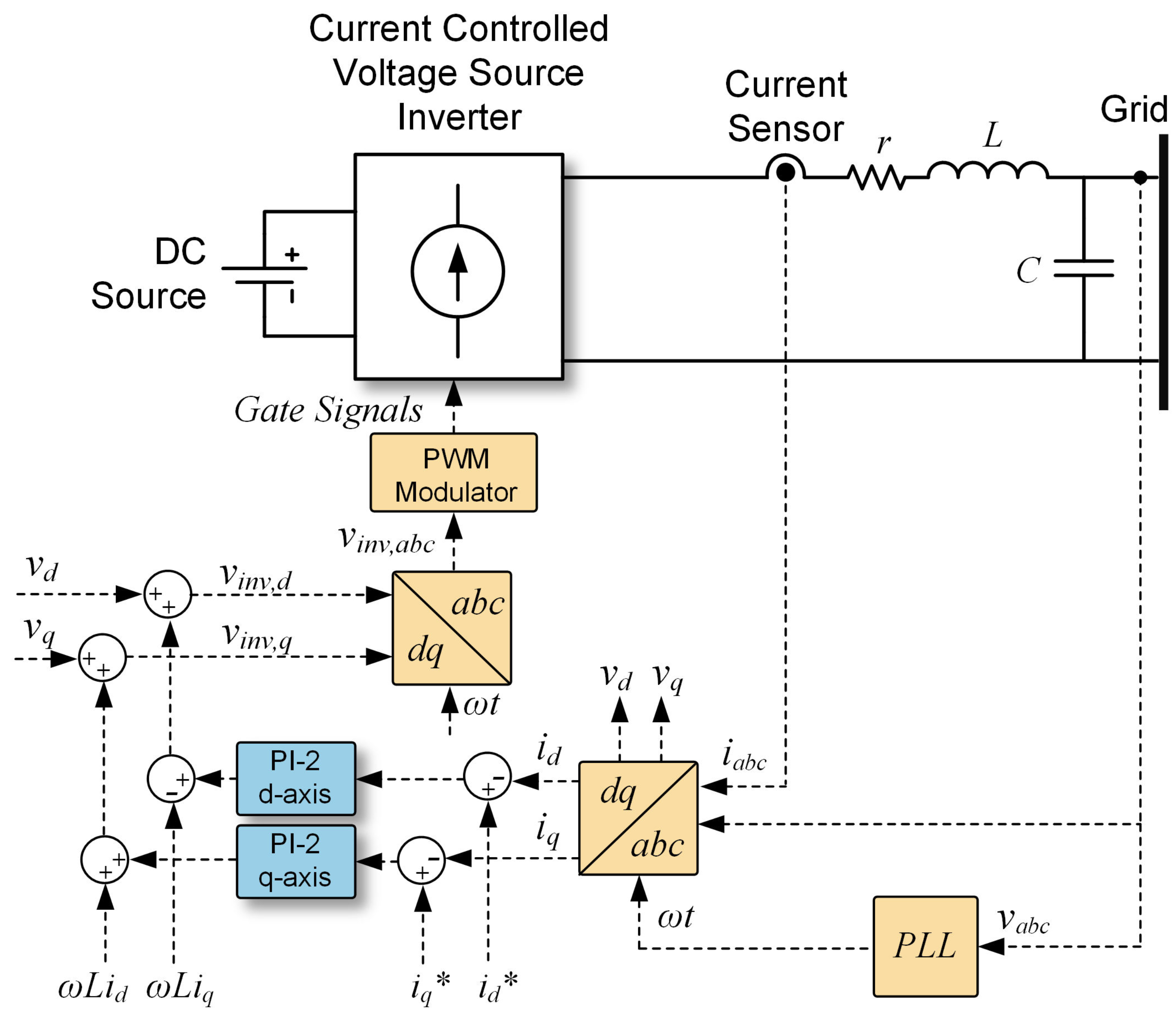
3. Design of Current Controllers

The simulation study of the current control techniques described in Section 2 was performed in MATLAB/Simulink using the parameters summarized in Table 1. The LC filter was designed for a cut-off frequency of 1 kHz, which is a decade below the switching frequency of 10 kHz to attenuate the high switching frequency noises generated by the inverter. For the PLL, typical parameters available in Simulink were used. The “Backward-Euler” technique in MATLAB/Simulink was used to discretize the simulations. The simulations were performed using MATLAB’s “ode23tb” variable-step solver.

3.1. PI (Proportional-Integral) Controller Design

Based on the parameters in Table 1 and using (2), the transfer function of the plant can derived as:
G p l a n t ( s ) = 100 s + 10
Figure 7a shows the frequency response of the plant, the designed PI Type-2 controller, and the loop transfer function of the overall designed system. The PI controller has a high gain at lower frequency regions, which ensures that the controller achieves a zero steady-state error. The controller was designed for a cut-off frequency of 1 kHz, which is a decade below the switching frequency (10 kHz). The controller bandwidth can theoretically be increased by designing the controller for a higher cut-off frequency; however, this will make the system susceptible to switching noises. The slope of the controller eventually decreases around the cut-off frequency region, ensuring the cut-off frequency specification is met. The controller rolls off at a higher slope at high frequency ranges to attenuate the switching noises. The phase margin of the loop transfer function (of the plant and the current controller combined) was selected to be 45 at the cross-over frequency of 1 kHz, which ensures an acceptable overshoot in the system response. The constants k P I , τ , and T p of (3) were thus calculated to be 62.93, 383.24 μ s, and 66.09 μ s, respectively, which corresponds to the following transfer function for the PI Type-2 controller:
C P I ( s ) = 62 . 96 s + 1 . 642 e 5 6 . 609 e 5 s 2 + s

3.2. PR (Proportional-Resonant) Controller

For the design of the PR controller, it is important to ensure that the controller can show zero steady-state error to signals at the resonant frequency, which in this case would be the grid frequency of 60 Hz. As such, the ω parameter in this design was taken to be 376.9 rad/s (60 Hz), and the ratio of the parameters, K I K P , was taken to be 300, which ensures that the resonant constant, K I , has a sufficiently high value. A high value of K I around the resonant frequency ensures the controller can exhibit near to zero steady-state error and track the 60-Hz sinusoidal signal accurately [22]. The constant K P was then calculated such that the resulting loop transfer function had a damping ratio of 0.42, which corresponds to a phase margin of 45 , as in the case of the PI controller designed previously. The calculated value of K P was 13.20. Figure 7 shows the frequency response of the plant, the designed PR controller, and the loop transfer function of the overall system. It can be observed that the controller has a high gain around the grid frequency of 60 Hz, as desired. Using these calculated values in (4), the transfer function of the designed PR controller was:
C P R ( s ) = 13 . 2 s 2 + 3960 s + 1 , 876 , 010 s 2 + 14 , 122

3.3. Hysteresis Controller Design

The hysteresis band controller was designed with a hysteresis band of 2% of the reference current. The hysteresis controller uses the same inductance values as the PI and PR controllers. No capacitance was connected before connecting the inverter to the grid.

3.4. Model Predictive Controller Design

For the design of the MPC, the parameters from Table 1 were used. The current prediction model described in (5) was used for predicting the one time step-ahead currents. The sampling time, T s , used in the simulation was 2 μ s. Similarly, the grid voltage required in (5) is estimated using (6). The predicted currents for each of the possible switching combinations is compared against the reference currents provided within the cost function minimization block. The cost function used in the design is the same as the one described in (7). Both the current prediction model and the cost function are implemented using the m function block within MATLAB/Simulink.

3.5. Supplementary ADP (Adaptive Dynamic Programming) Controller Design

The input of the action network is designed as: X ( t ) = [ x 1 , x 2 , x 3 , x 4 , x 5 , x 6 ] , where x 1 is the error signal between i d * and i d , x 2 and x 3 are the one-time step and two-time step delayed signals, x 4 is the error signal between i q * and i q , and x 5 and x 6 are one-time step and two-time step delayed signals as shown in Figure 6a. Therefore, the architecture of the action network in ADP is designed as a 6-6-2 multi-layer perceptron (MLP) structure, and the critic network is designed as an 8-6-1 MLP structure with six hidden neurons for each network. The output of the ADP controller is the control action, u ( t ) = [ u d ( t ) , u q ( t ) ] , where u d ( t ) and u q ( t ) are control actions for the d-axis and q-axis, which supplements the output of the PI controller. The reward signal is designed as:
r ( t ) = c i = 1 6 a i x i 2 ,
where c, a i for i = 1,...,6 are the coefficients of this quadratic equation. The weights of the two networks are updated using the gradient descent algorithm described in [49]. The typical learning process of the ADP controller includes two trials, as described in [50]. In the first trial, the neural networks were initialized with random weights, and the supplementary control action outputs may not be optimal. The simulations were repeated until there was no further improvement in the total harmonic distortion (THD). At the end of this offline learning process, the ADP learns information about the system and state-action pairs. In the second trial, or online learning, fully-trained control policies in terms of trained weights were used that obtain better control performance over time. After enough training, the actor produced the optimal control action and the critic evaluated the performance of the actor over time.

4. Simulation Results and Comparative Analysis

The simulation results of each of the current control techniques will be presented first, followed by a thorough comparative analysis. For analysis of each of the current control techniques, the d-axis current command was changed from 2 A–6 A at a simulation time of 0.05 s in all cases. This represents the change in reference current, which would be generated from the outer loop with the virtual inertia algorithm in a full implementation. The q-axis current was kept constant at zero through the simulation. The simulation results for each controller are described first, followed by sections on transient performance and harmonic performance comparison.

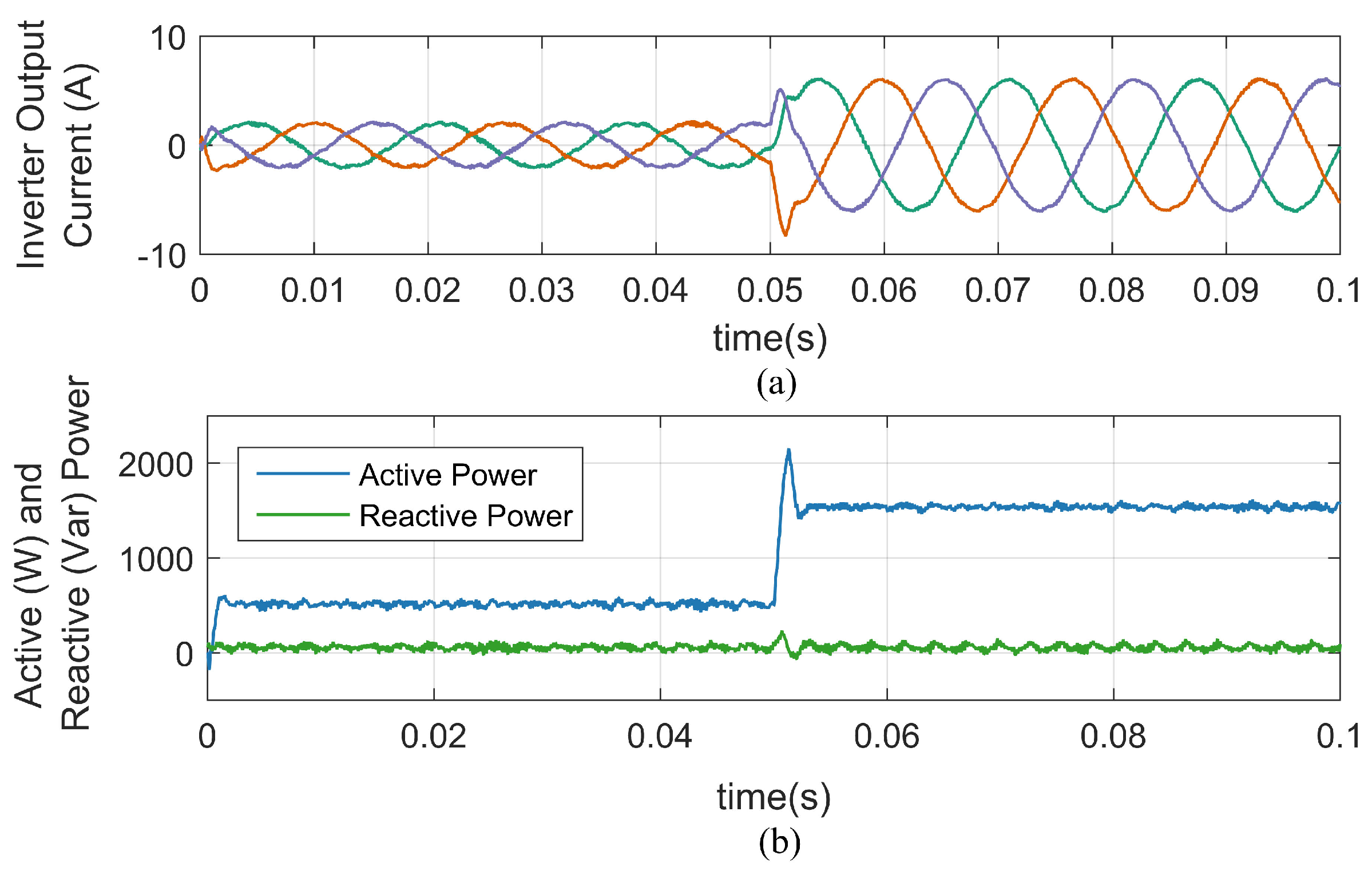
4.1. PI Controller Simulation Results

The output current of the grid-connected inverter when a PI controller was used in the current control loop is shown in Figure 8a. During the change in the reference current command at 0.05 s, the shape of the current waveform was slightly distorted during the transient, but quickly recovered to maintain a sinusoidal shape. The change in d-axis current means that the output power of the inverter changed from 500–1500 W, as shown in Figure 8b. There was an overshoot of 40% in the active power response, which was slightly higher than expected for a PI controller designed with a phase margin of 45°. This can be attributed to the peaks from the switching of the converter. Such an overshoot can be critical for larger systems, as the inverters need to be over-sized, which ultimately increases the cost. The overshoots can theoretically be minimized in the control design phase, but would result in a slower speed response. The reactive power, however, remained constant at around 50 Var (average) throughout the simulation as the q-axis reference was kept at 0 A. There was a short transient pickup in the reactive power when the active power changed.

4.2. PR Controller Simulation Results

The output current of the grid-connected inverter when a PR controller was used in the current control is shown in Figure 9a. With the PR controller, during the change in the reference current command at 0.05 s, there was no distortion in the shape of the current waveform as in the case of the PI controller. In addition, a closer observation of the current waveform, especially for a lower references, shows lower distortion compared to that with a PI controller. Figure 9b shows the change in the active power of the grid-connected inverter corresponding to the change in the output current. The response time was similar to that of the PI controller, but the overshoot was only 8% in this case. This could be beneficial for virtual inertia implementation, as this could greatly reduce the cost of the components, as less overshoot has to be handled by the inverter. In large systems, even this small reduction in the overshoot can translate to significant economic savings.

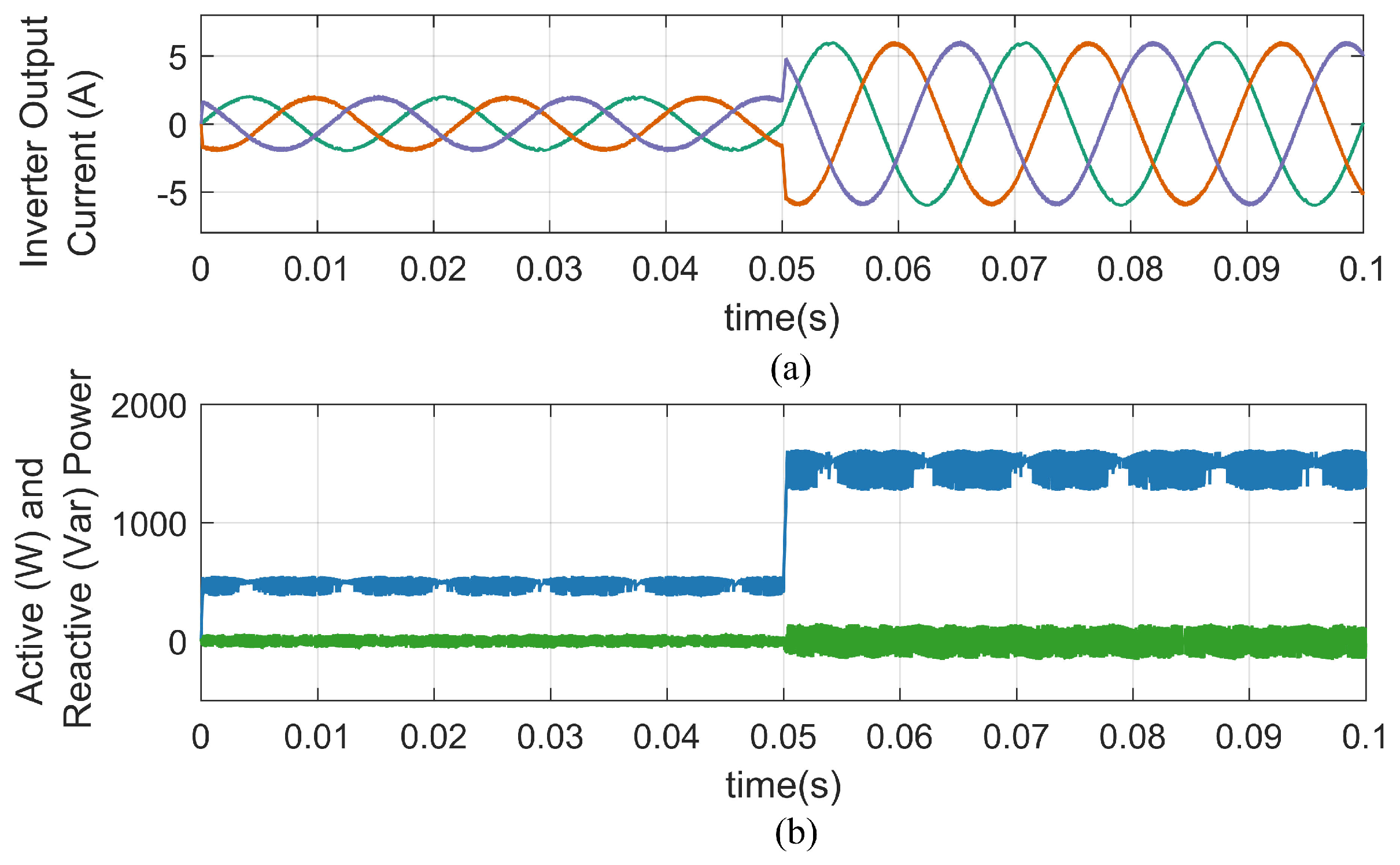
4.3. Hysteresis Controller Simulation Results

The output current of the grid-connected inverter when a hysteresis controller was used in the current control loop is shown in Figure 10a. Similar to the PR controller, in this case, the transition of current during the step change in current reference was smooth without any distortions. Figure 10b shows the change in the active power of the grid-connected inverter corresponding to the change in the output current. The response speed of the output power was quicker than both the PI and PR controllers. Moreover, the overshoot in the active power response was negligible. One disadvantage, however, is that there was increased ripple in both the active and reactive power output, which can be attributed as an effect of the variable switching frequency of this type of controller. Moreover, the ripple seemed to increase for higher values of reference currents.

4.4. Model Predictive Controller Simulation Results

The output current of the grid-connected inverter when a MPC was used in the current control loop is shown in Figure 11a. As with the case of PR and hysteresis control, during the step change in the reference current, there were no distortions. Figure 11b shows the change in the active power of the grid-connected inverter corresponding to the change in the output current. The response speed of the output power was the fastest among PI, PR, and hysteresis control, which was suitable for virtual inertia emulation, as discussed previously. The frequency of a weak grid with lower inertia can decrease/increase quickly, and the additional required inertia has to be emulated almost instantaneously to prevent significant changes in frequency [51]. The fast response of the MPC technique can be exploited for this effect. However, the absence of a modulator and the variable switching operation means both the active and reactive power have a higher output ripple. Moreover, the high switching frequencies generated may lead to increased system losses.

4.5. Supplementary ADP Controller Simulation Results

The output current of the grid-connected inverter when a supplementary ADP control approach was used in the current control loop is shown in Figure 12a. The main objective of the controller is to improve the transient performance of a traditional PI controller. It is worth noting here that the neural network does not completely replace the original PI controller, but only supplements the generated control actions. Figure 12b shows the change in the active power of the grid-connected inverter corresponding to the change in the output current. The overshoot in the active power in this case was reduced to about 26% while improving the response time. This reduction as stated before can bring economic savings. It is also worth noting that the ADP control actions did not increase the switching frequency, as in the case of the hysteresis and MPC controllers.

4.6. Transient Response Comparison

Figure 13 shows the transient response of d-axis and q-axis currents for different current control techniques, along with the percent of overshoot and response time ( t r ), which is the time taken by the response signal to increase from 10–90% of the final value. For the PI controller, there was a significant overshoot of 40%, and the response time was the slowest among all the controllers. The PR controller was able to achieve a lower overshoot of 8% with a slightly faster response time, while the overshoot was negligible at 1% with the hysteresis controller. The MPC controller, on the other hand, was able to achieve both of these objectives of a low overshoot and fast response time (about 50% reduction in response time), but at the cost of a higher average switching frequency about three-times higher than the PI and PR controller. The supplementary ADP was able to reduce the overshoot to 26% from the 40% value of the PI controller with a similar response time. However, the main advantage with this approach is that there was no increase in the switching frequency as in the case of MPC. Moreover, the constant frequency with ADP controller means the harmonics in the current are predictable and can be filtered out easily.

4.7. Harmonic Contents Comparison

Figure 14 presents a comparison of the frequency spectrum of the output current of the grid-connected inverter along with respective THD values. Table 2 summarizes the performance of the different current control techniques discussed in this paper in terms of the THD, overshoot, response time, and number of switching that occurred per 60-Hz AC cycle. The THD was calculated using six full AC cycles of the output current waveform as recommended in IEEE std. 519 [52]. When using the PI controller, the THD was highest among all the controllers at 2.30%, but the constant switching frequency means that the lower order harmonics, which are of the most concern, were concentrated together, which makes the processes of filtering out these harmonics easier. The PR controller was able to achieve a lower THD of 1.01%, and the harmonics were concentrated around lower order as in the case of the PI controller. With the hysteresis and the MPC controllers, on other hand, the frequency spectrum was widespread because of the variable switching frequency. Although the THD values were quite low at 1.60% and 1.35%, respectively, there may be difficulties in the filter design while implementing these controllers. The supplementary controller was able to reduce the overshoot in the response, while achieving a lower THD of 1.68% and response time than that of a PI controller. The THD was however higher than with the hysteresis and/or the MPC control.

5. Conclusions

The design and comparative performance analysis of the PI, PR, hysteresis, MPC, and the supplementary ADP controller were presented in this paper. Simulation studies showed that the PI Type-2 controller had a slow response and high overshoot and was not suitable for virtual inertia systems. The oversizing of the inverters required to handle these overshoots can become an economic barrier. The PR controller on the other hand showed a lower overshoot for a similar response time. However, the performance may deteriorate in weak grids (or microgrids), where the system frequency can deviate by a substantial amount. The hysteresis control and the MPC present robust control options with minimal overshoot and fast response times. However, they suffer from the disadvantages of a variable switching frequency unless appropriate improvements are made in the controller to address these issues. The integration of a supplementary ADP controller was able to reduce the overshoots while achieving a similar response time as the PI and PR controllers. Moreover, the switching frequency remained constant, unlike the hysteresis and MPC controllers. Hence, from the point of view of implementation simplicity, the PI, PR, and hysteresis control appear to be good choices. In weak grids, where the frequency of the system can drop in a very short time, the hysteresis or even the MPC technique with fast response may be more desirable. If the hysteresis or the MPC control approaches are used, proper care needs to be taken in the filter design. Moreover, the MPC will demand higher computational power and improved semiconductor switches. Integrating the traditional PI controller with the ADP can combine the advantage of the PI controller with a lower overshoot and may be more robust in weak grids than PR controllers.

Author Contributions

Conceptualization, I.T. and R.T.; formal analysis, U.T. and I.T.; funding acquisition, T.M.H. and R.T.; investigation, U.T., D.S. and N.M.; methodology, U.T., D.S., N.M., I.T. and R.T.; project administration, R.T.; validation, U.T. and Z.N.; visualization, Z.N. and T.M.H.; writing, original draft, U.T., D.S. and N.M.; writing, review and editing, Z.N., T.M.H., I.T. and R.T.

Funding

This research was funded by South Dakota State University’s (SDSU) Department of Electrical Engineering and Computer Science PhD Funding, South Dakota Board of Regents (SDBoR) and the National Science Foundation (NSF) under Grant Number ECCS-1608722 and the NSF Major Research Instrumentation (MRI) under the Grant Number MRI-1726964 and Microsoft.

Acknowledgments

This paper is an expanded version of our work in [10]. The authors would like to thank Department of Electrical Engineering and Computer Science at South Dakota State University (SDSU) for providing the laboratory resources to perform the studies.

Conflicts of Interest

The authors declare no conflict of interest.

Abbreviations

The following abbreviations are used in this manuscript:
ADPAdaptive dynamic programming
CC-VSICurrent-controlled voltage source inverter
DSPDigital signal processors
ESSEnergy storage system
FCS-MPCFinite control set model predictive control
FPGAField programmable gate array
MLPMulti-layer perceptron
MPCModel predictive control
PIProportional integral
PLLPhase-locked loop
PRProportional resonant
NERCNorth American Electric Reliability Corporation
PIProportional-integral
PVPhotovoltaic
RESRenewable energy system
ROCOF    Rate of change of frequency

References

  1. Kroposki, B.; Mather, B. Rise of Distributed Power: Integrating Solar Energy into the Grid [Guest Editorial]. IEEE Power Energy Mag. 2015, 13, 14–18. [Google Scholar] [CrossRef]
  2. Fang, J.; Li, H.; Tang, Y.; Blaabjerg, F. Distributed power system virtual inertia implemented by grid-connected power converters. IEEE Trans. Power Electron. 2018, 33, 8488–8499. [Google Scholar] [CrossRef]
  3. Tielens, P.; Van Hertem, D. Grid inertia and frequency control in power systems with high penetration of renewables. In Proceedings of the Young Researchers Symposium in Electrical Power Engineering, Delft, The Netherlands, 16–17 April 2012. [Google Scholar]
  4. Tamrakar, U.; Galipeau, D.; Tonkoski, R.; Tamrakar, I. Improving transient stability of photovoltaic-hydro microgrids using virtual synchronous machines. In Proceedings of the IEEE Eindhoven PowerTech, Eindhoven, The Netherlands, 29 June–2 July 2015; pp. 1–6. [Google Scholar]
  5. Shrestha, D.; Tamrakar, U.; Malla, N.; Ni, Z.; Tonkoski, R. Reduction of energy consumption of virtual synchronous machine using supplementary adaptive dynamic programming. In Proceedings of the IEEE International Conference on Electro Information Technology (EIT), Grand Forks, ND, USA, 19–21 May 2016; pp. 690–694. [Google Scholar] [CrossRef]
  6. Beck, H.P.; Hesse, R. Virtual synchronous machine. In Proceedings of the International Conference on Electrical Power Quality and Utilisation, Barcelona, Spain, 9–11 October 2007. [Google Scholar]
  7. Alipoor, J.; Miura, Y.; Ise, T. Power System Stabilization Using Virtual Synchronous Generator With Alternating Moment of Inertia. IEEE J. Emerg. Sel. Top. Power Electron. 2015, 3, 451–458. [Google Scholar] [CrossRef]
  8. Zhong, Q.C.; Weiss, G. Synchronverters: Inverters That Mimic Synchronous Generators. IEEE Trans. Ind. Electron. 2011, 58, 1259–1267. [Google Scholar] [CrossRef]
  9. Zhang, W.; Cantarellas, A.M.; Rocabert, J.; Luna, A.; Rodriguez, P. Synchronous Power Controller With Flexible Droop Characteristics for Renewable Power Generation Systems. IEEE Trans. Sustain. Energy 2016, 7, 1572–1582. [Google Scholar] [CrossRef]
  10. Tamrakar, U.; Tonkoski, R.; Ni, Z.; Hansen, T.M.; Tamrakar, I. Current control techniques for applications in virtual synchronous machines. In Proceedings of the IEEE 6th International Conference on Power Systems (ICPS), New Delhi, India, 4–6 March 2016. [Google Scholar] [CrossRef]
  11. Kassakian, J.G.; Jahns, T.M. Evolving and Emerging Applications of Power Electronics in Systems. IEEE J. Emerg. Sel. Top. Power Electron. 2013, 1, 47–58. [Google Scholar] [CrossRef]
  12. Vazquez, S.; Leon, J.I.; Franquelo, L.G.; Rodriguez, J.; Young, H.A.; Marquez, A.; Zanchetta, P. Model Predictive Control: A Review of Its Applications in Power Electronics. IEEE Ind. Electron. Mag. 2014, 8, 16–31. [Google Scholar] [CrossRef] [Green Version]
  13. Malla, N.; Shrestha, D.; Ni, Z.; Tonkoski, R. Supplementary control for virtual synchronous machine based on adaptive dynamic programming. In Proceedings of the IEEE Congress on Evolutionary Computation (CEC), Vancouver, BC, Canada, 24–29 July 2016; pp. 1998–2005. [Google Scholar] [CrossRef]
  14. Malla, N.; Tamrakar, U.; Shrestha, D.; Ni, Z.; Tonkoski, R. Online learning control for harmonics reduction based on current controlled voltage source power inverters. IEEE/CAA J. Autom. Sin. 2017, 4, 447–457. [Google Scholar] [CrossRef]
  15. Sakimoto, K.; Miura, Y.; Ise, T. Stabilization of a power system with a distributed generator by a Virtual Synchronous Generator function. In Proceedings of the 8th International Conference on Power Electronics—ECCE Asia, Jeju, South Korea, 30 May–3 June 2011; pp. 1498–1505. [Google Scholar] [CrossRef]
  16. D’Arco, S.; Suul, J.A. Virtual synchronous machines—Classification of implementations and analysis of equivalence to droop controllers for microgrids. In Proceedings of the 2013 IEEE Grenoble PowerTech (POWERTECH), Grenoble, France, 16–20 June 2013; pp. 1–7. [Google Scholar]
  17. Bevrani, H.; Ise, T.; Miura, Y. Virtual synchronous generators: A survey and new perspectives. Int. J. Electr. Power Energy Syst. 2014, 54, 244–254. [Google Scholar] [CrossRef]
  18. Tamrakar, U.; Shrestha, D.; Maharjan, M.; Bhattarai, B.; Hansen, T.; Tonkoski, R. Virtual inertia: Current trends and future directions. Appl. Sci. 2017, 7, 654. [Google Scholar] [CrossRef]
  19. Cha, H.; Vu, T.K.; Kim, J.E. Design and control of Proportional-Resonant controller based Photovoltaic power conditioning system. In Proceedings of the IEEE Energy Conversion Congress and Exposition (ECCE), San Jose, CA, USA, 20–24 September 2009; pp. 2198–2205. [Google Scholar]
  20. Blaabjerg, F.; Teodorescu, R.; Liserre, M.; Timbus, A.V. Overview of Control and Grid Synchronization for Distributed Power Generation Systems. IEEE Trans. Ind. Electron. 2006, 53, 1398–1409. [Google Scholar] [CrossRef] [Green Version]
  21. He, J.; Li, Y.W.; Blaabjerg, F.; Wang, X. Active harmonic filtering using current-controlled, grid-connected DG units with closed-loop power control. IEEE Trans. Power Electron. 2014, 29, 642–653. [Google Scholar]
  22. Zhong, Q.C.; Hornik, T. Control of Power Inverters in Renewable Energy and Smart Grid Integration; John Wiley & Sons: Hoboken, NJ, USA, 2012; Volume 97. [Google Scholar]
  23. Dannehl, J.; Wessels, C.; Fuchs, F.W. Limitations of voltage-oriented PI current control of grid-connected PWM rectifiers with LCL filters. IEEE Trans. Ind. Electron. 2009, 56, 380–388. [Google Scholar] [CrossRef]
  24. Vasquez, J.C.; Guerrero, J.M.; Savaghebi, M.; Eloy-Garcia, J.; Teodorescu, R. Modeling, analysis, and design of stationary-reference-frame droop-controlled parallel three-phase voltage source inverters. IEEE Trans. Ind. Electron. 2013, 60, 1271–1280. [Google Scholar] [CrossRef]
  25. Timbus, A.V.; Ciobotaru, M.; Teodorescu, R.; Blaabjerg, F. Adaptive resonant controller for grid-connected converters in distributed power generation systems. In Proceedings of the 21st Annual IEEE Applied Power Electronics Conference and Exposition (APEC), Dallas, TX, USA, 19–23 March 2006. [Google Scholar] [CrossRef]
  26. Sato, Y.; Ishizuka, T.; Nezu, K.; Kataoka, T. A new control strategy for voltage-type PWM rectifiers to realize zero steady-state control error in input current. IEEE Trans. Ind. Appl. 1998, 34, 480–486. [Google Scholar] [CrossRef]
  27. Davoodnezhad, R.; Holmes, D.; McGrath, B. A fully digital hysteresis current controller for current regulation of grid connected PV inverters. In Proceedings of the 2014 IEEE 5th International Symposium on Power Electronics for Distributed Generation Systems (PEDG), Galway, Ireland, 24–27 June 2014; pp. 1–8. [Google Scholar]
  28. Wu, F.; Zhang, L.; Wu, Q. Simple unipolar maximum switching frequency limited hysteresis current control for grid-connected inverter. IET Power Electron. 2014, 7, 933–945. [Google Scholar] [CrossRef]
  29. Suul, J.A.; Ljokelsoy, K.; Midtsund, T.; Undeland, T. Synchronous Reference Frame Hysteresis Current Control for Grid Converter Applications. IEEE Trans. Ind. Appl. 2011, 47, 2183–2194. [Google Scholar] [CrossRef]
  30. Davoodnezhad, R.; Holmes, D.G.; McGrath, B.P. A novel three-level hysteresis current regulation strategy for three-phase three-level inverters. IEEE Trans. Power Electron. 2014, 29, 6100–6109. [Google Scholar] [CrossRef]
  31. Wu, F.; Feng, F.; Luo, L.; Duan, J.; Sun, L. Sampling period online adjusting-based hysteresis current control without band with constant switching frequency. IEEE Trans. Ind. Electron. 2015, 62, 270–277. [Google Scholar] [CrossRef]
  32. Zhang, J.; Yang, H.; Wang, T.; Li, L.; Dorrell, D.G.; Lu, D.D.C. Field-oriented control based on hysteresis band current controller for a permanent magnet synchronous motor driven by a direct matrix converter. IET Power Electron. 2018, 11, 1277–1285. [Google Scholar] [CrossRef]
  33. Tamrakar, I.; Shilpakar, L.; Fernandes, B.; Nilsen, R. Voltage and frequency control of parallel operated synchronous generator and induction generator with STATCOM in micro hydro scheme. IET Gener. Trans. Distrib. 2007, 1, 743–750. [Google Scholar] [CrossRef]
  34. Bolognani, S.; Bolognani, S.; Peretti, L.; Zigliotto, M. Design and Implementation of Model Predictive Control for Electrical Motor Drives. IEEE Trans. Ind. Electron. 2009, 56, 1925–1936. [Google Scholar] [CrossRef]
  35. Rodriguez, J.; Kazmierkowski, M.P.; Espinoza, J.R.; Zanchetta, P.; Abu-Rub, H.; Young, H.A.; Rojas, C.A. State of the Art of Finite Control Set Model Predictive Control in Power Electronics. IEEE Trans. Ind. Inf. 2013, 9, 1003–1016. [Google Scholar] [CrossRef]
  36. Zhang, Y.; Peng, Y.; Qu, C. Model Predictive Control and Direct Power Control for PWM Rectifiers With Active Power Ripple Minimization. IEEE Trans. Ind. Appl. 2016, 52, 4909–4918. [Google Scholar] [CrossRef]
  37. Rodriguez, J.; Pontt, J.; Silva, C.A.; Correa, P.; Lezana, P.; Cortés, P.; Ammann, U. Predictive current control of a voltage source inverter. IEEE Trans. Ind. Electron. 2007, 54, 495–503. [Google Scholar] [CrossRef]
  38. Cortes, P.; Kazmierkowski, M.P.; Kennel, R.M.; Quevedo, D.E.; Rodriguez, J. Predictive Control in Power Electronics and Drives. IEEE Trans. Ind. Electron. 2008, 55, 4312–4324. [Google Scholar] [CrossRef]
  39. Aguilera, R.P.; Lezana, P.; Quevedo, D.E. Finite-Control-Set Model Predictive Control With Improved Steady-State Performance. IEEE Trans. Ind. Inf. 2013, 9, 658–667. [Google Scholar] [CrossRef]
  40. Kouro, S.; Cortes, P.; Vargas, R.; Ammann, U.; Rodriguez, J. Model Predictive Control—A Simple and Powerful Method to Control Power Converters. IEEE Trans. Ind. Electron. 2009, 56, 1826–1838. [Google Scholar] [CrossRef]
  41. Drobnic, K.; Nemec, M.; Nedeljkovic, D.; Ambrozic, V. Predictive Direct Control Applied to AC Drives and Active Power Filter. IEEE Trans. Ind. Electron. 2009, 56, 1884–1893. [Google Scholar] [CrossRef]
  42. Young, H.A.; Perez, M.A.; Rodriguez, J. Analysis of Finite-Control-Set Model Predictive Current Control With Model Parameter Mismatch in a Three-Phase Inverter. IEEE Trans. Ind. Electron. 2016, 63, 3100–3107. [Google Scholar] [CrossRef]
  43. Bellman, R. Dynamic Programming; Princeton University Press: Princeton, NJ, USA, 1957. [Google Scholar]
  44. Lewis, F.; Liu, D. (Eds.) Reinforcement Learning and Approximate Dynamic Programming for Feedback Control; Wiley-IEEE Press: Piscataway, NJ, USA, 2013. [Google Scholar]
  45. Si, J.; Barto, A.G.; Powell, W.B.; Wunsch, D.C. (Eds.) Handbook of Learning and Approximate Dynamic Programming; Wiley-IEEE Press: Piscataway, NJ, USA, 2004. [Google Scholar]
  46. He, H.; Ni, Z.; Fu, J. A Three-Network Architecture for On-Line Learning and Optimization based on Adaptive Dynamic Programming. Neurocomputing 2012, 78, 3–13. [Google Scholar] [CrossRef]
  47. Guo, W.; Liu, F.; Si, J.; He, D.; Harley, R.; Mei, S. Approximate dynamic programming based supplementary reactive power control for DFIG wind farm to enhance power system stability. Neurocomputing 2015, 170, 417–427. [Google Scholar] [CrossRef]
  48. Zhang, H.G.; Zhang, X.; Yan-Hong, L.; Jun, Y. An overview of research on adaptive dynamic programming. Acta Autom. Sin. 2013, 39, 303–311. [Google Scholar] [CrossRef]
  49. Si, J.; Wang, Y.T. Online learning control by association and reinforcement. IEEE Trans. Neural Netw. 2001, 12, 264–276. [Google Scholar] [CrossRef] [PubMed] [Green Version]
  50. Lu, C.; Si, J.; Xie, X. Direct heuristic dynamic programming for damping oscillations in a large power system. IEEE Trans. Syst. Man Cybern. Part B (Cybern.) 2008, 38, 1008–1013. [Google Scholar]
  51. Ulbig, A.; Borsche, T.S.; Andersson, G. Impact of low rotational inertia on power system stability and operation. IFAC Proc. Vol. 2014, 47, 7290–7297. [Google Scholar] [CrossRef]
  52. IEEE Recommended Practices and Requirements for Harmonic Control in Electrical Power Systems; IEEE Std 519-1992; IEEE: Piscataway, NJ, USA, 2014.
Figure 1. Operating principle of a virtual inertia emulation system.
Applsci 08 02695 g001
Figure 2. Schematic diagram of the grid-connected inverter benchmark and PI (proportional-integral) Type-2 based current controller; PLL: Phase Locked Loop; PWM: Pulse Width Modulation; “*” represents the reference values of the signals.
Applsci 08 02695 g002
Figure 3. Schematic diagram of a PR-based current controller; PR: proportional-resonant; PWM: pulse width modulation; “*” represents the reference values of the signals.
Applsci 08 02695 g003
Figure 4. Hysteresis current controller. (a) Schematic diagram. (b) gate signal generation.
Applsci 08 02695 g004
Figure 5. Model predictive controller. (a) Schematic diagram. (b) detailed structure.
Applsci 08 02695 g005
Figure 6. Supplementary ADP (adaptive dynamic programming) controller. (a) Schematic diagram. (b) detailed structure showing the action and critic network.
Applsci 08 02695 g006
Figure 7. Frequency response of the plant, the designed controller, and the loop transfer function (LTF) of the overall system. (a) PI Type-2 controller. (b) PR controller.
Applsci 08 02695 g007
Figure 8. Simulation results with the PI controller. (a) Three-phase output current of the inverter. (b) Active and reactive power output.
Applsci 08 02695 g008
Figure 9. Simulation results with PR controller. (a) Three-phase output current of inverter. (b) Active and reactive power output.
Applsci 08 02695 g009
Figure 10. Simulation results with hysteresis controller. (a) Three-phase output current of inverter. (b) Active and reactive power output.
Applsci 08 02695 g010
Figure 11. Simulation results with MPC. (a) Three-phase output current of inverter. (b) Active and reactive power output.
Applsci 08 02695 g011
Figure 12. Simulation results with the ADP controller. (a) Three-phase output current of inverter. (b) Active and reactive power output.
Applsci 08 02695 g012
Figure 13. Comparison of d-axis and q-axis current responses. (a) PI controller. (b) PR controller. (c) Hysteresis controller. (d) MPC. (e) Supplementary ADP controller; O.S.: Overshoot.
Applsci 08 02695 g013
Figure 14. Comparison of the harmonic spectrum of the output current. (a) PI controller. (b) PR controller. (c) Hysteresis controller. (d) MPC. (e) Supplementary ADP controller. THD: Total Harmonic Distortion.
Applsci 08 02695 g014
Table 1. Simulation parameters; PI: proportional-integral; PR: proportional-resonant; ADP: adaptive dynamic programming.
ParametersValues
DC Voltage ( V D C )400 V
Grid Frequency (f)60 Hz
Grid Voltage ( V g )208 V (L-L)
Grid Impedance ( Z g r i d ) ( 0.135 + j 0.169 ) Ω
Switching Frequency (PI, PR, and ADP) ( f s w )10 kHz
Switch Dead-time ( t d )2 μ s
Filter Inductance (L)10 mH
Filter Resistance (r)0.1 Ω
Filter Capacitance (C)3.3 μ F
Table 2. Performance comparison of current controllers.
ControllerTHDOvershootResponse Time ( μ s)Switching/Cycle
PI2.30%40.5%492333
PR1.02%8.2%462333
Hysteresis1.60%1.0%447669
MPC1.35%0.9%238935
ADP1.68%26.1%465333

