Influence of Three-Dimensional Coral Structures on Hyperspectral Benthic Reflectance and Water-Leaving Reflectance


Abstract
Featured Application
Abstract
1. Introduction
- Investigate how the spectral reflectance at the scale of coral macro-morphology (shape) relates to coral surface-scale spectral reflectance.
- Quantify the error arising from making simplifying modelling assumptions, such as using a single reflectance spectrum to represent a coral under different light environments, or excluding water attenuation and scattering between coral structures within the canopy.
- Characterize the BRDF of assemblages of corals in different densities.
- Apply those BRDFs as the bottom boundary in HydroLight, to model BRDF effects in the remote sensing reflectance arising from canopy BRDF properties in different depths and conditions.
2. Materials and Methods
2.1. Overview
2.2. Coral Surface Reflectances and Shape
2.3. Radiative Transfer Modelling
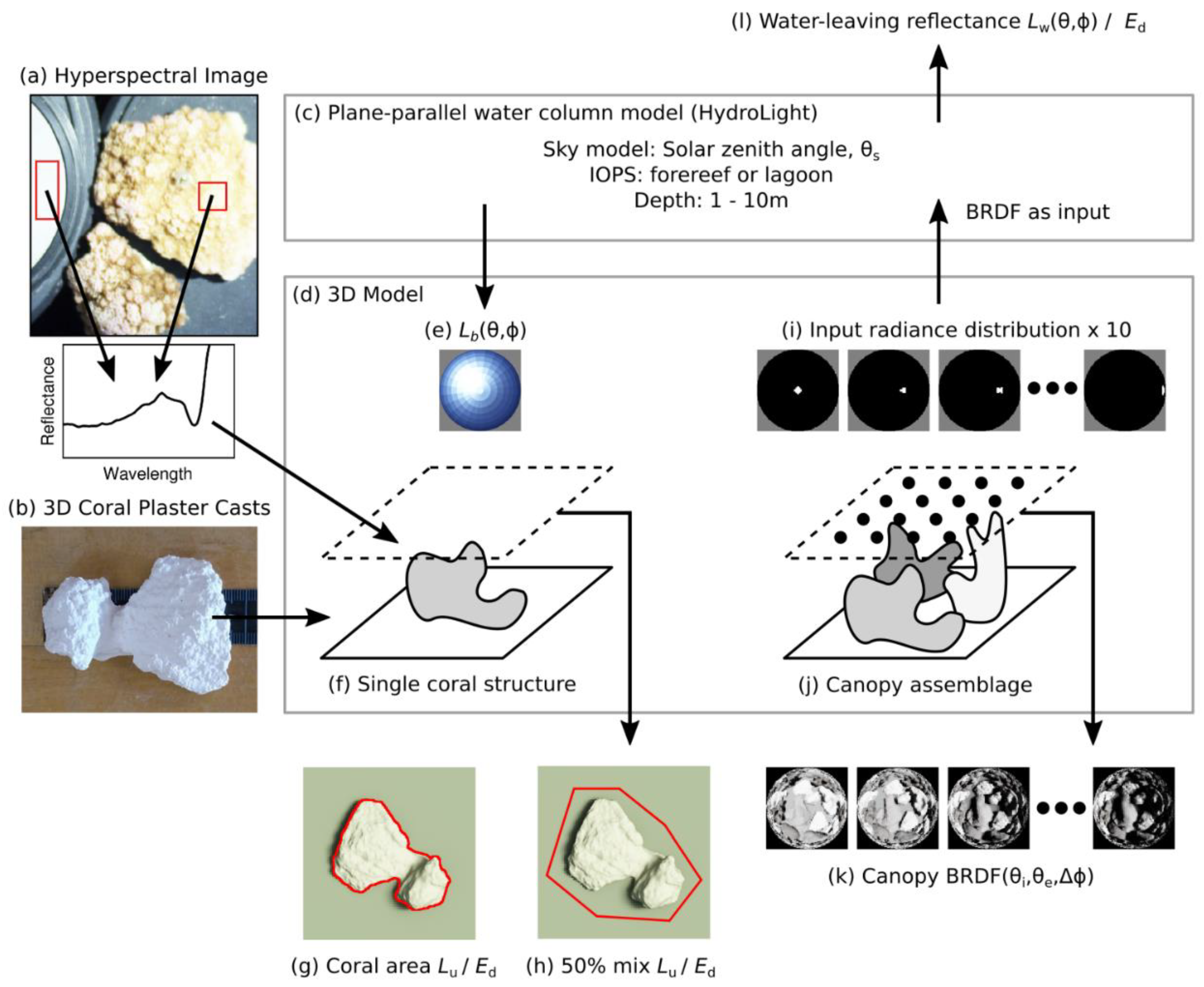
- HydroLight was used to generate a bottom of water column radiance distribution, and this was used to illuminate the individual coral structures, standing on flat dead coral substrate, by being used as the input radiance boundary condition (Figure 1e,f). From these model runs, the reflectance over the coral structure was determined under different illumination conditions to deduce the average reflectance and its variability due to shading and other effects, across a range of illumination conditions (Figure 1g,h). Treatments were applied corresponding to the range limits of interest: Depths of 1 m and 10 m; solar zenith angles of 10° and 50°, azimuth angles of 0°, 90°, 180°, 270°, and two sets of Inherent Optical Properties (IOPs) denoted “forereef” and “lagoon” (described below). Water surface roughness was set to correspond to a wind speed of 5 ms−1 but note that only water leaving radiance was used in the results, so surface reflectance was excluded. This method was used for tests 1 to 4, listed in Table 1.
- Mixtures of 3D living coral structures were assembled on flat dead coral rock substrate, in areal cover densities from 39% to 75%. The 3D model was used with horizontal periodic boundaries to generate a canopy BRDF function, which was then used as a bottom boundary condition in HydroLight (Figure 1i,j). By this method, spectral water-leaving reflectances derived as water-leaving radiance at a given wavelength (λ) normalized to downwelling planar irradiance (Lw(θ, Δφ, λ)/Ed(λ)), could be derived above the water for different view directions under different solar zenith angles and water column conditions (Figure 1l). Incorporating the water column this way spatially averages the results, and scope of the results corresponds to pixels larger than the coral structures, i.e., pixels ≥ 1 m, since the coral structures were less than 20 cm across. This modelling covered the same range of depths, solar zenith angles, and the two IOP treatments mentioned above. This aspect of the work corresponds to activities 5 and 6 in Table 1.
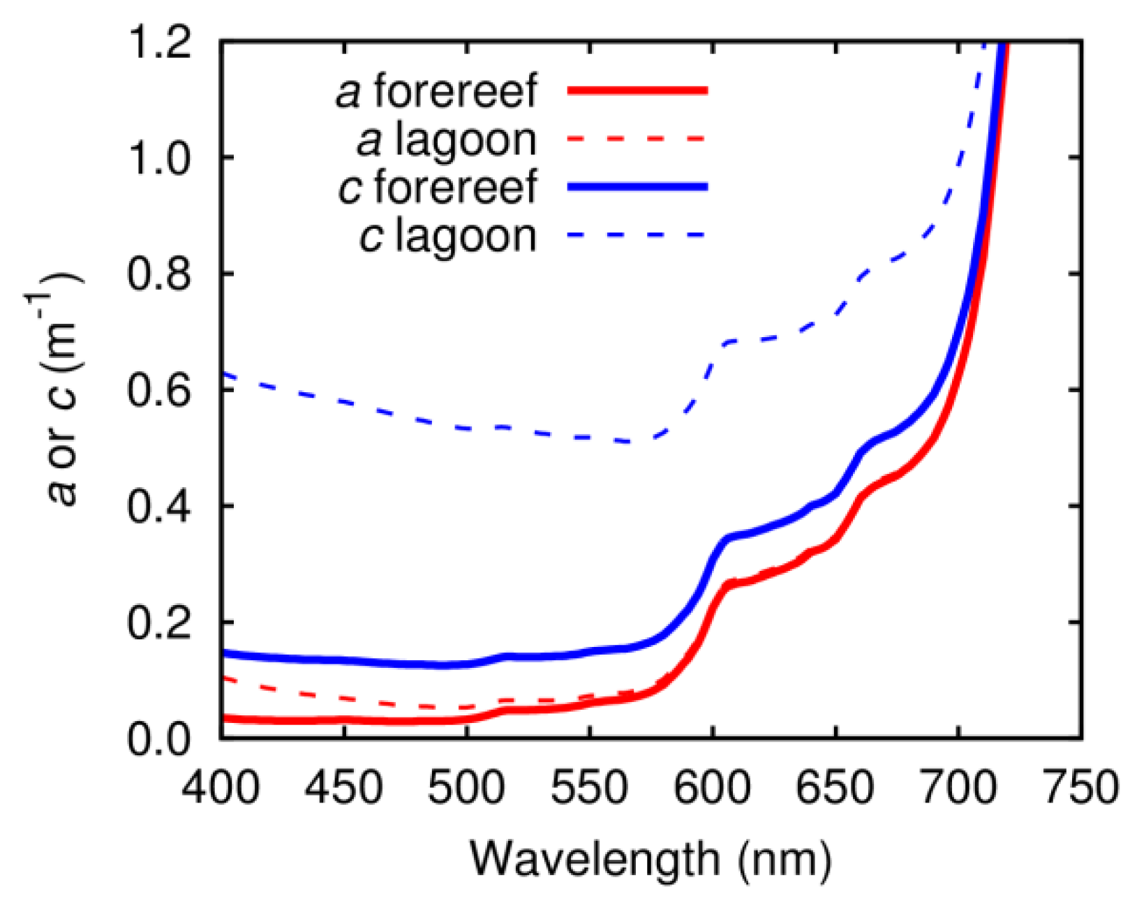
2.4. Inherent Optical Properties
2.5. Coral Canopy Assemblages
2.6. Coral Model Outputs and Processing
3. Results and Discussion
3.1. Effect of Coral Shape on Nadir View Reflectance
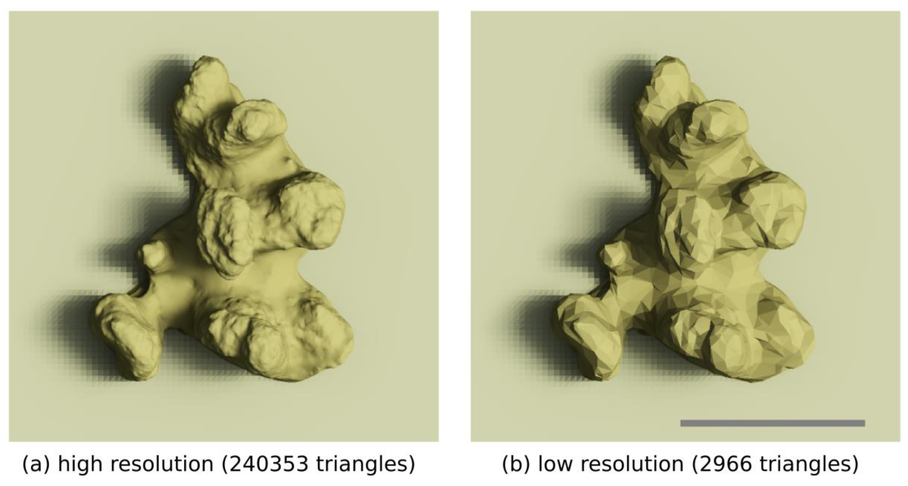
3.2. Effect of 3D Model Resolution
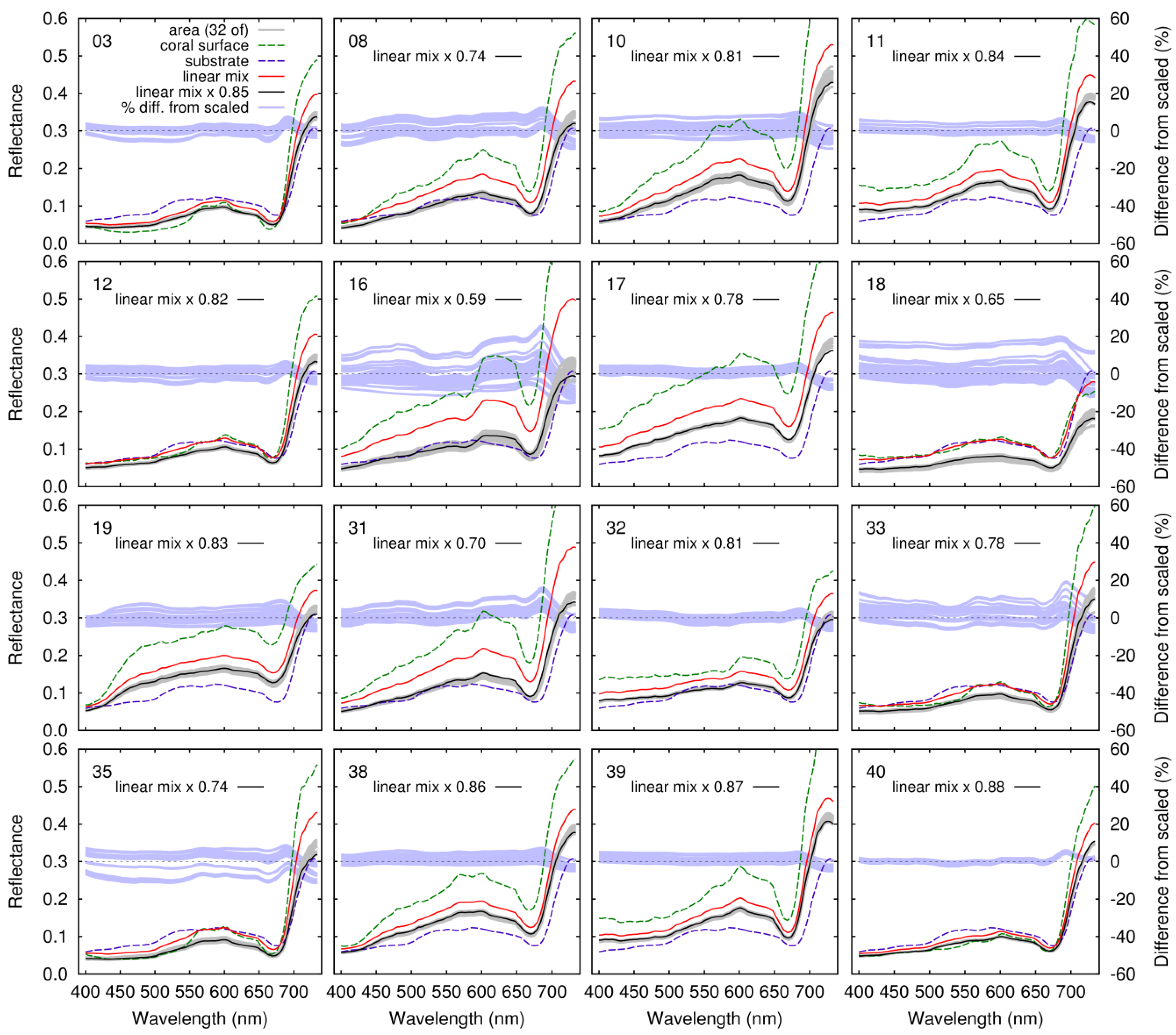
3.3. Linear Mixing of Reflectance over Coral Shapes and Surrounding Substrate
3.4. Effect of Interstitial Scattering and Absorption
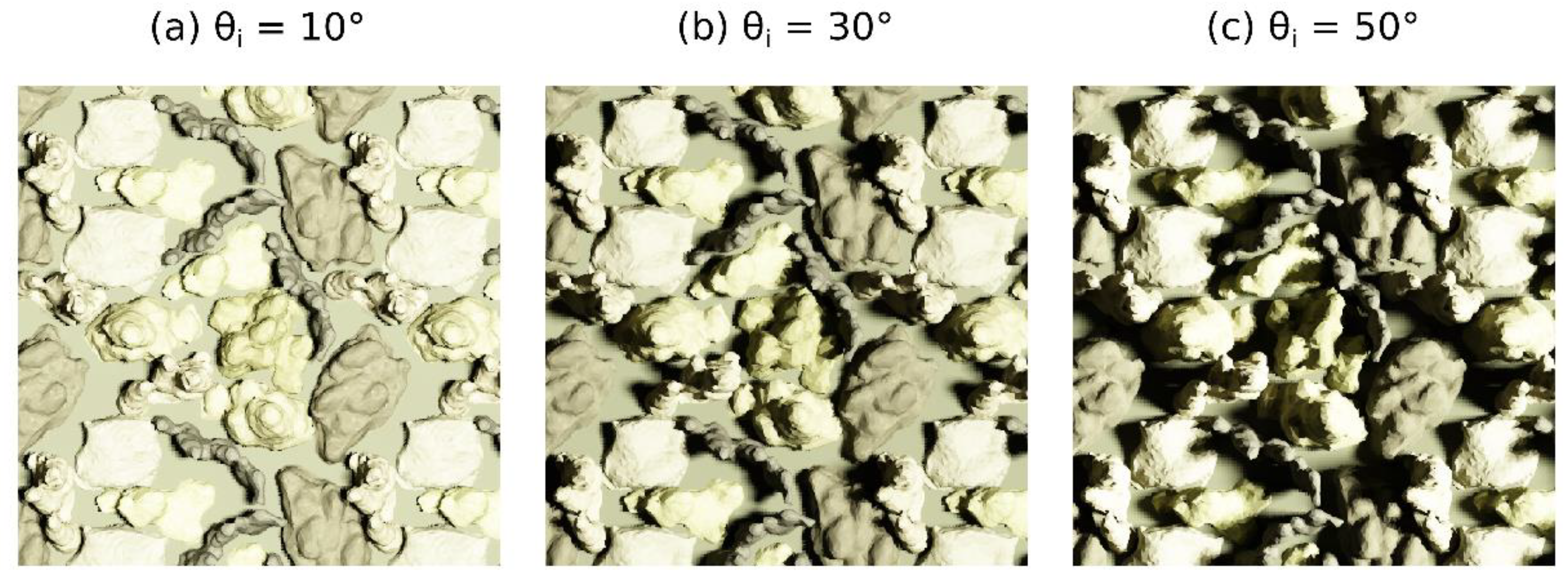
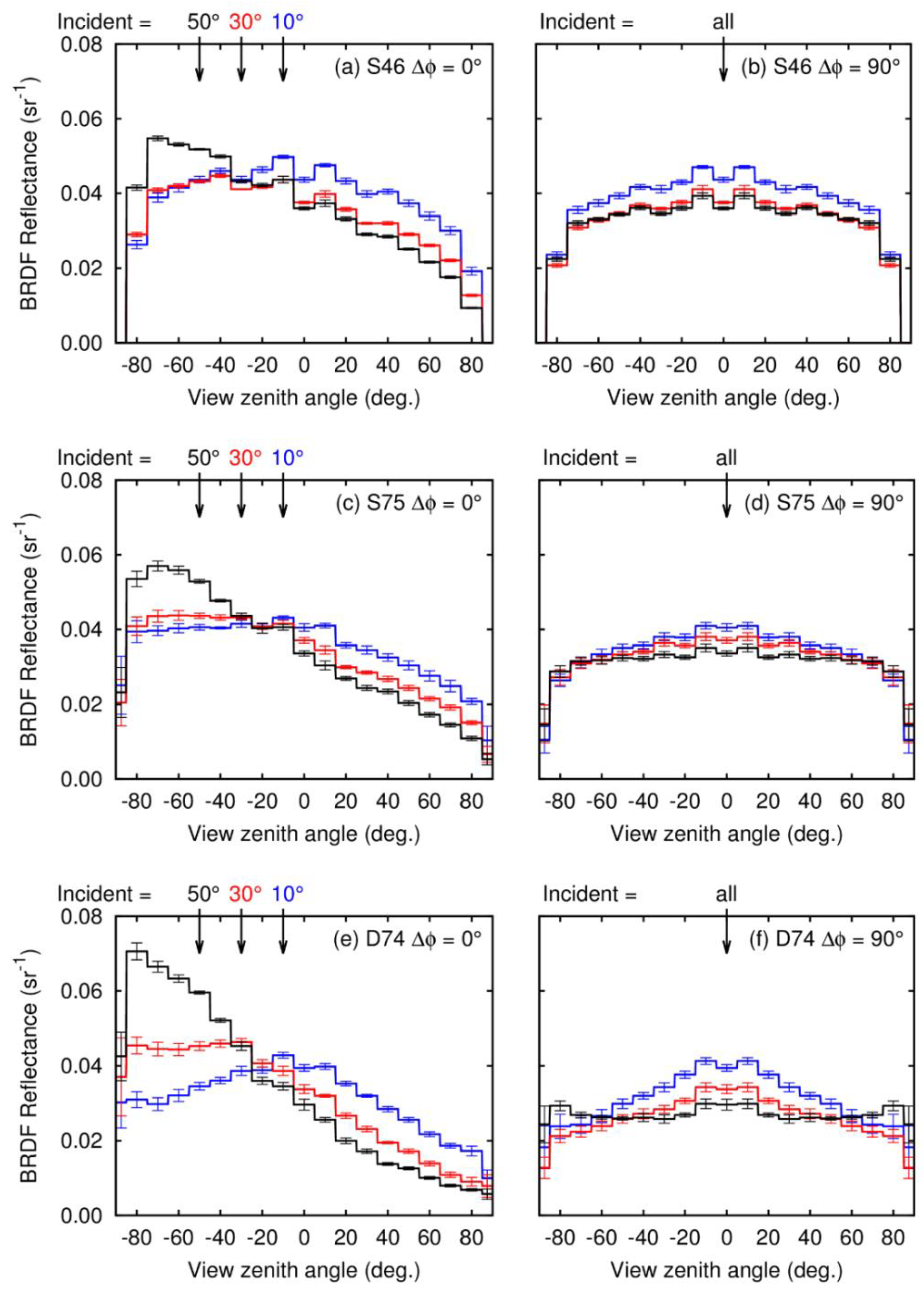
3.5. Canopy Assemblage BRDF Effects
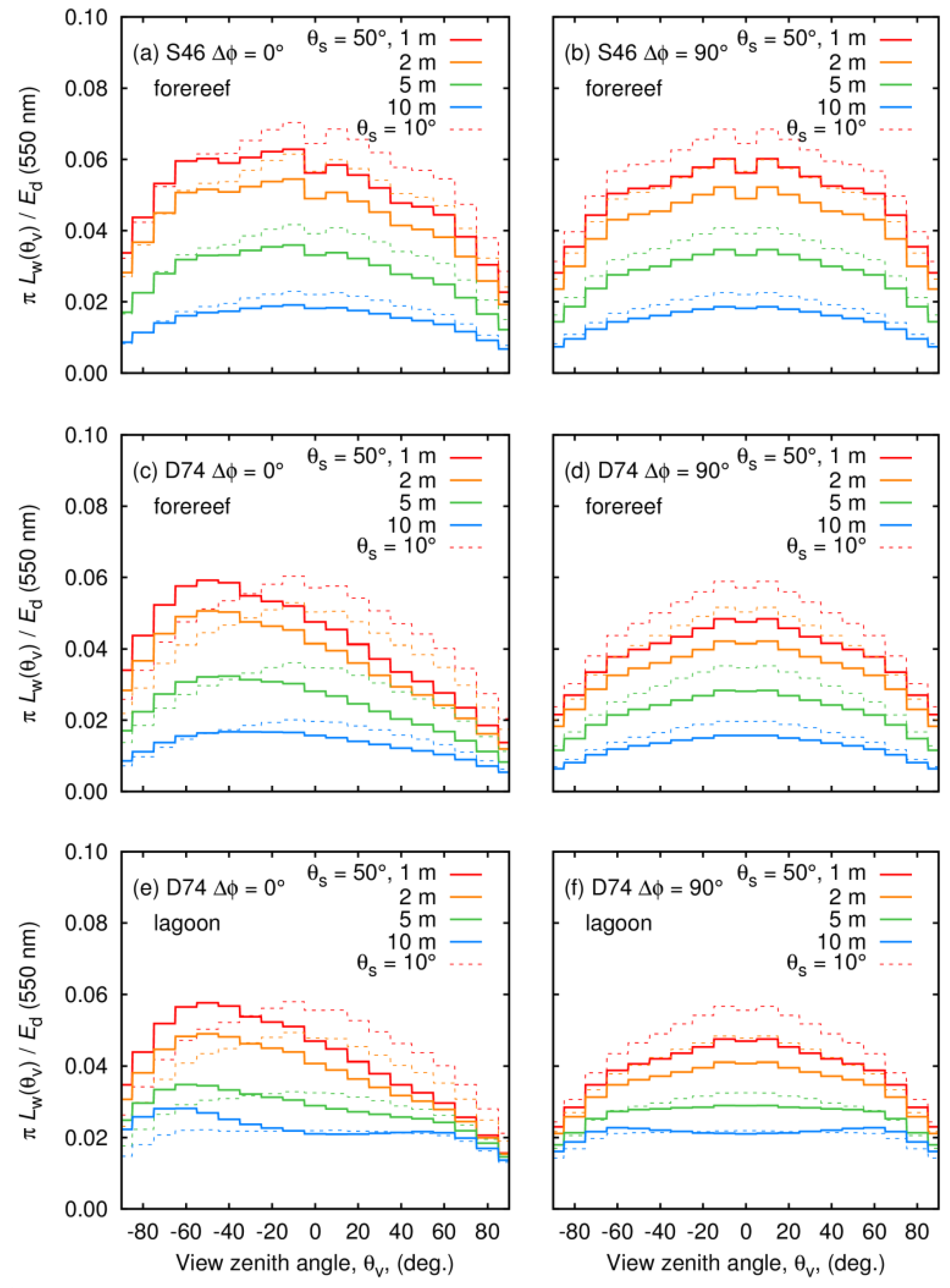
3.6. Above-Water BRDF Effects
4. Conclusions
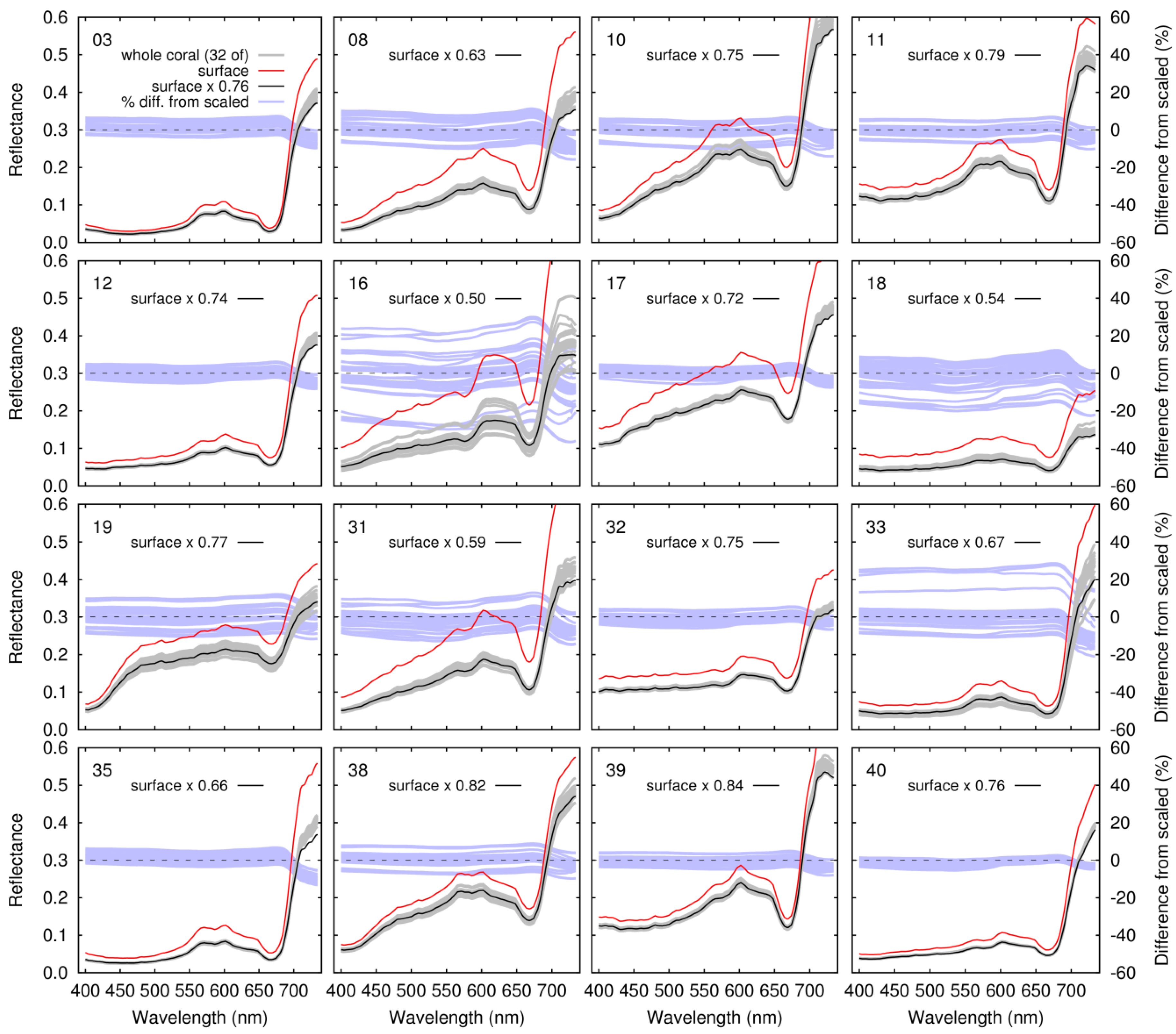
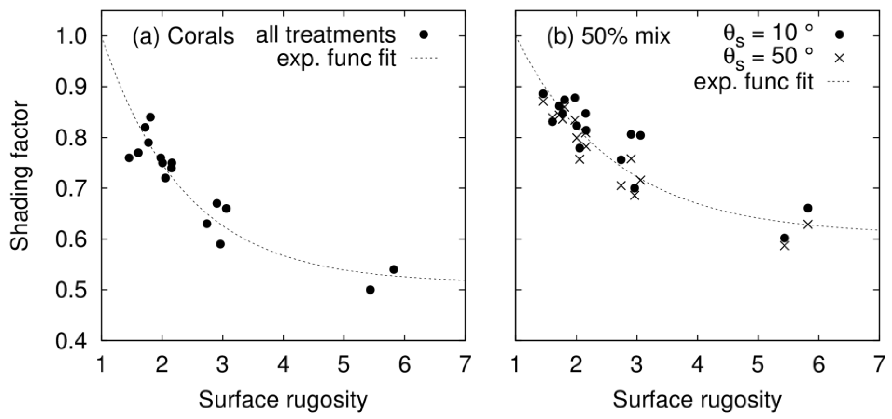
- If the input reflectances for different benthic types can be considered ‘pure’ surface reflectances, then structural complexity implies the introduction of a shading scale factor or a black shade endmember in mixing models is required. In our data, that shading scale factor could be anywhere from 0.5 to 0.9, whereas for a genuinely flat substrate it would be 1.0.
- The magnitude of the shading factor is inversely related to surface rugosity; hence the shade factor value could be set based on the expected bottom types, or if derivable in an image analysis, it would give additional information on benthic type.
- Nadir viewing reflectance over the bottom (Lu/Ed) for individual corals varies as much as ~20% (more only in exceptional cases) under the range of light environments found on reefs, under typical remote sensing conditions.
- Regarding view directions beyond a few 10s of degrees from nadir for dense canopies in shallow water shading, hotspot effects become relevant, leading to potentially a 50% difference (factor of 1.5) in above water reflectance. At narrower remote sensing geometries (view zenith angles < 20°), differences can be 20% (factor of 1.2).
- For all modelled canopy assemblages, there were only small BRDF effects at a relative viewing angle of 90° to the incident solar plane. The advice for minimizing cross-track BRDF effects in airborne imagery is therefore consistent with that for minimizing surface glint, i.e., fly in a direction close to the solar plane with a solar zenith angle greater than 30°.
- Collection of in-situ spectra of benthic types requires consideration of what level of shading is already included, or whether the data is close to being a surface reflectance measurement. However, including shading in field measurements cannot fully accommodate the influence of canopy interactions, because there are effects at canopy scale involving different benthic types.
- These modelling results provide useful concepts and parameter ranges, which can assist in the interpretation of empirical data and the development of image processing algorithms.
Author Contributions
Funding
Acknowledgments
Conflicts of Interest
References
- Hedley, J.D.; Roelfsema, C.M.; Chollet-Ordaz, I.; Harborne, A.R.; Heron, S.F.; Weeks, S.; Skirving, W.J.; Strong, A.E.; Eakin, C.M.; Christensen, T.R.L.; et al. Remote sensing of coral reefs for monitoring and management: A review. Remote Sens. 2016, 8, 118. [Google Scholar] [CrossRef]
- Mumby, P.J.; Skirving, W.; Strong, A.E.; Hardy, J.T.; LeDrew, E.F.; Hochberg, E.J.; Stumpf, R.P.; David, L.T. Remote sensing of coral reefs and their physical environment. Mar. Pollut. Bull. 2004, 48, 219–228. [Google Scholar] [CrossRef] [PubMed]
- Mumby, P.J.; Green, E.P.; Edwards, A.J.; Clark, C.D. Coral reef habitat-mapping: How much detail can remote sensing provide? Mar. Biol. 1997, 130, 193–202. [Google Scholar] [CrossRef]
- Hochberg, E.J.; Atkinson, M.J. Capabilities of remote sensors to classify coral, algae, and sand as pure and mixed spectra. Remote Sens. Environ. 2003, 85, 174–189. [Google Scholar] [CrossRef]
- Capolsini, P.; Andréfouët, S.; Rion, C.; Payri, C. A comparison of Landsat ETM+, SPOT HRV, Ikonos, ASTER, and airborne MASTER data for coral reef habitat mapping in South Pacific islands. Can. J. Remote Sens. 2007, 23, 87–200. [Google Scholar] [CrossRef]
- Lubin, D.; Li, W.; Dustan, P.; Mazel, C.H.; Stamnes, K. Spectral Signatures of coral reefs: Features from space. Remote Sens. Environ. 2001, 75, 127–137. [Google Scholar] [CrossRef]
- Hedley, J.D.; Roelfsema, C.; Phinn, S.R.; Mumby, P.J. Environmental and sensor limitations in optical remote sensing of coral reefs: Implications for monitoring and sensor design. Remote Sens. 2012, 4, 271–302. [Google Scholar] [CrossRef]
- Hedley, J.D.; Mumby, P.J. Biological and remote sensing perspectives of pigmentation in coral reef organisms. Adv. Mar. Biol. 2002, 43, 277–317. [Google Scholar] [PubMed]
- Mumby, P.J.; Hedley, J.D.; Chisholm, J.R.M.; Clark, C.D.; Ripley, H.; Jaubert, J. The cover of living and dead corals from airborne remote sensing. Coral Reefs 2004, 23, 171–183. [Google Scholar] [CrossRef]
- Goodman, J.A.; Ustin, S.L. Classification of benthic composition in a coral reef environment using spectral unmixing. J. Appl. Remote Sens. 2007, 1, 011501. [Google Scholar]
- Hochberg, E.J.; Atkinson, M.J. Spectral discrimination of coral reef benthic communities. Coral Reefs 2000, 19, 164–171. [Google Scholar] [CrossRef]
- Lesser, M.P.; Mobley, C.D. Bathymetry, water optical properties, and benthic classification of coral reefs using hyperspectral remote sensing imagery. Coral Reefs 2007, 26, 819–829. [Google Scholar] [CrossRef]
- Leiper, I.A.; Phinn, S.R.; Roelfsema, C.M.; Joyce, K.E.; Dekker, A.G. Mapping Coral Reef Benthos, Substrates, and Bathymetry, Using Compact Airborne Spectrographic Imager (CASI) Data. Remote Sens. 2014, 6, 6423–6445. [Google Scholar] [CrossRef]
- Garcia, R.A.; Lee, Z.; Hochberg, E.J. Hyperspectral Shallow-Water Remote Sensing with an Enhanced Benthic Classifier. Remote Sens. 2018, 10, 147. [Google Scholar] [CrossRef]
- Joyce, K.E.; Phinn, S.R. Bi-directional reflectance of corals. Int. J. Remote Sens. 2002, 23, 389–394. [Google Scholar] [CrossRef]
- Miller, I.; Foster, B.C.; Laffan, S.W.; Brander, R.W. Bidirectional reflectance of coral growth-forms. Int. J. Remote Sens. 2016, 37, 1553–1567. [Google Scholar] [CrossRef]
- Hedley, J.D.; Mumby, P.J.; Joyce, K.E.; Phinn, S.R. Spectral unmixing of coral reef benthos under ideal conditions. Coral Reefs 2004, 23, 60–73. [Google Scholar] [CrossRef]
- Hedley, J.D. A three-dimensional radiative transfer model for shallow water environments. Optics Express 2008, 16, 21887–21902. [Google Scholar] [CrossRef] [PubMed]
- Mobley, C.D.; Sundman, L. Hydrolight 5.2 User’s Guide. Sequoia Scientific. Available online: https://www.sequoiasci.com/wp-content/uploads/2013/07/HE52UsersGuide.pdf (accessed on 25 July 2018).
- Young, G.C.; Dey, S.; Rogers, A.D.; Exton, D. Cost and time-effective method for multi-scale measures of rugosity, fractal dimension, and vector dispersion from coral reef 3D models. PLoS ONE 2017, 12, e0175341. [Google Scholar] [CrossRef] [PubMed]
- Hedley, J.D.; Enríquez, S. Optical properties of canopies of the tropical seagrass Thalassia testudinum estimated by a three-dimensional radiative transfer model. Limnol. Oceanogr. 2010, 55, 1537–1550. [Google Scholar] [CrossRef]
- Hedley, J.D.; McMahon, K.; Fearns, P. Seagrass canopy photosynthetic response is a function of canopy density and light environment: A model for Amphibolis griffithi. PloS ONE 2014, 9, e111454. [Google Scholar] [CrossRef] [PubMed]
- Hedley, J.D.; Russell, B.; Randolph, K.; Dierssen, H. A physics-based method for the remote sensing of seagrasses. Remote Sens. Environ. 2015, 174, 134–147. [Google Scholar] [CrossRef]
- Mobley, C.D. Light and Water: Radiative Transfer in Natural Waters; Academic Press: San Diego, CA, USA, 1994; ISBN 0-12-502750-8. [Google Scholar]
- Russell, A.B.; Hochberg, E.; Dierssen, H.M. Comparison of water column optical properties across geomorphic zones of Pacific coral reefs. Limnol. Oceanogr. under review.
- Adams, J.B.; Smith, M.O.; Johnson, P.E. Spectral mixture modelling: A new analysis of rock and soil types at the Viking Lander I site. J. Geophys. Res. 1986, 91, 8098–8112. [Google Scholar] [CrossRef]
- Dekker, A.G.; Phinn, S.R.; Anstee, J.; Bissett, P.; Brando, V.E.; Casey, B.; Fearns, P.; Hedley, J.; Klonowski, W.; Lee, Z.P.; et al. Intercomparison of shallow water bathymetry, hydro–optics, and benthos mapping techniques in Australian and Caribbean coastal environments. Limnol. Oceanogr. Methods 2011, 9, 396–425. [Google Scholar] [CrossRef]
- Roelfsema, C.M.; Marshall, J.; Phinn, S.R.; Joyce, K. Underwater Spectrometer System 2006 (UWSS04)—Manual; Biophysical Remote Sensing Group, Centre for Spatial Environmental Research, University of Queensland: Queensland, Australia, 2006. [Google Scholar]
- Roelfsema, C.M.; Phinn, S.R. Spectral Reflectance Library of Healthy and Bleached Corals in the Keppel Islands, Great Barrier Reef. PANGAEA. Available online: https://doi.org/10.1594/PANGAEA.872507 (accessed on 25 July 2018).
- Liang, S. Quantitative Remote Sensing of Land Surfaces; Wiley: Hoboken, NJ, USA, 2004; ISBN 978-0471281665. [Google Scholar]
- Mobley, C.D.; Zhang, H.; Voss, K.J. Effects of optically shallow bottoms on upwelling radiances: Bidirectional reflectance distribution function effects. Limnol. Oceanogr. 2003, 48, 337–345. [Google Scholar] [CrossRef]
- Kay, S.; Hedley, J.D.; Lavender, S. Sun glint correction of high and low spatial resolution images of aquatic scenes: A review of methods for visible and near-infrared wavelengths. Remote Sens. 2009, 1, 697–730. [Google Scholar] [CrossRef]


| Modelled Property | Res. | I. | Derived Reflectance and Purpose of Activity | Position | |
|---|---|---|---|---|---|
| 1 | Reflectance averaged over each of the 16 coral shapes, for the coral area only (substrate masked out). Bottom of water column incident radiance distribution generated by HydroLight with 32 treatments, combining: Solar zenith angles 10° and 50°; depths 1 m and 10 m; forereef and lagoon IOPs; and four rotational positions of the coral shape. | high | N | π Lu/Ed Effect of shape on reflectance over coral area only. | above canopy |
| 2 | low | N | π Lu/Ed Effect of resolution of 3D models. | above canopy | |
| 3 | Reflectance averaged over a single coral shape, plus in each case, surrounding substrate to give a 50% mix in terms of areal cover. Incident radiance distributions as above. | low | N | π Lu/Ed Validity of linear mixing model for reflectance over coral and surrounding substrate. | above canopy |
| 4 | low | Y | π Lu/Ed Effect of ignoring water scattering and attenuation within canopy. | above canopy | |
| 5 | Azimuthally averaged BRDF function for six canopy assemblages ranging from 39% to 75% coral cover. BRDF tabulated in HydroLight standard directional discretization. | low | N | π BRDF(θi, θe, Δφ) Demonstrate canopy BRDF effects and generate function for input to HydroLight. | above canopy |
| 6 | Above-water remote sensing reflectance as a function of solar-view geometry, depth, and IOPs, for six canopy BRDFs generated as above. | low | N | π Lw(θs, θv, Δφ)/Ed Demonstrate above water BRDF effects under typical solar-view geometries. | above water |
| ID | Species | Polygon Count | Rugosity | Max Lu/Ed Difference | ||
|---|---|---|---|---|---|---|
| Group | Low Res. | High Res. | Low vs. High | |||
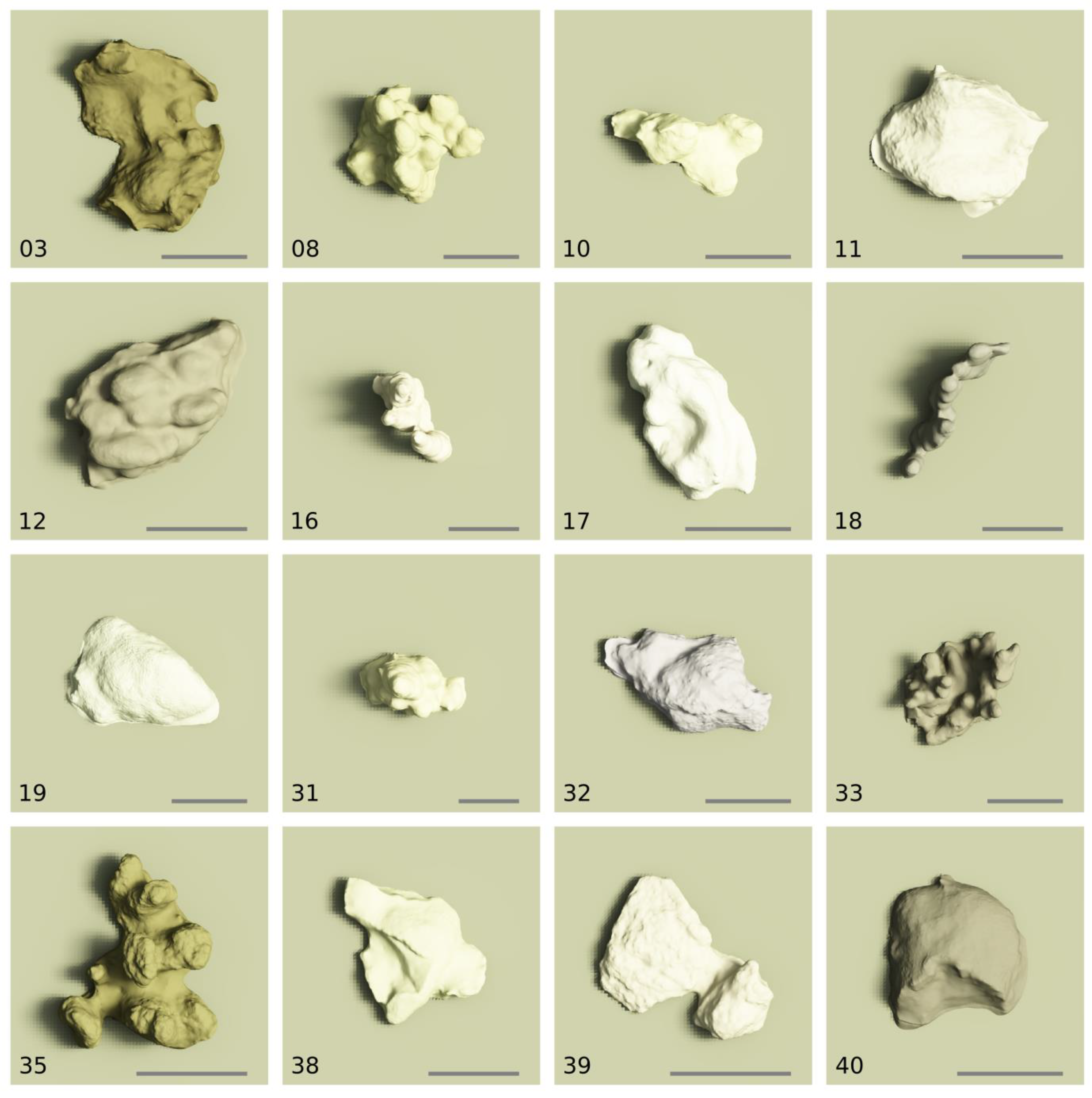
| 03 | Montipora capitata | n/a | 2306 | 152,185 | 1.98 | 0.36 |
| 08 | Porites evermanni | D | 1712 | 69,945 | 2.74 | 0.51 |
| 10 | Porites evermanni | D | 1832 | 75,524 | 2.16 | 0.28 |
| 11 | Montipora capitata | D | 1830 | 103,394 | 1.77 | 0.29 |
| 12 | Porites evermanni | D | 2150 | 51,954 | 2.16 | 0.24 |
| 16 | Porites compressa | D | 1454 | 89,703 | 5.43 | 1.33 |
| 17 | Porites evermanni | S | 2079 | 124,092 | 2.05 | 0.27 |
| 18 | Porites compressa | D | 1898 | 103,430 | 5.82 | 0.47 |
| 19 | Porites evermanni | S | 1804 | 183,283 | 1.61 | 0.22 |
| 31 | Porites compressa | D | 1226 | 56,726 | 2.96 | 0.43 |
| 32 | Montipora capitata | S | 2461 | 100,886 | 2.01 | 0.31 |
| 33 | Porites compressa | S | 2160 | 98,502 | 2.90 | 0.47 |
| 35 | Pocillopora sp. | S | 2966 | 240,353 | 3.06 | 0.21 |
| 38 | Porites evermanni or lutea | S | 1908 | 95,265 | 1.72 | 0.17 |
| 39 | Montipora patula | S | 2264 | 133,594 | 1.81 | 0.39 |
| 40 | Porites evermanni or lutea | S | 1403 | 56,696 | 1.45 | 0.17 |
| ID | Species | Shading Scale Factor Coral only | Shading Scale Factor 50% Coral-Substrate Mix | Max Lu/Ed diff. with Interstitial IOPs (≤690 nm) | ||
|---|---|---|---|---|---|---|
| Range | Median | Range | Median | |||
| 03 | Montipora capitata | 0.71–0.79 | 0.76 | 0.83–0.88 | 0.85 | 2.6% |
| 08 | Porites evermanni | 0.57–0.69 | 0.63 | 0.68–0.77 | 0.74 | 2.8% |
| 10 | Porites evermanni | 0.71–0.82 | 0.75 | 0.75–0.84 | 0.81 | 1.6% |
| 11 | Montipora capitata | 0.75–0.84 | 0.79 | 0.80–0.85 | 0.84 | 1.0% |
| 12 | Porites evermanni | 0.71–0.77 | 0.74 | 0.79–0.85 | 0.82 | 1.7% |
| 16 | Porites compressa | 0.39–0.66 | 0.50 | 0.51–0.64 | 0.59 | 3.1% |
| 17 | Porites evermanni | 0.69–0.75 | 0.72 | 0.75–0.79 | 0.78 | 1.0% |
| 18 | Porites compressa | 0.50–0.65 | 0.54 | 0.55–0.68 | 0.65 | 3.0% |
| 19 | Porites evermanni | 0.69–0.85 | 0.77 | 0.78–0.86 | 0.83 | 1.9% |
| 31 | Porites compressa | 0.54–0.65 | 0.59 | 0.64–0.71 | 0.70 | 2.8% |
| 32 | Montipora capitata | 0.72–0.78 | 0.75 | 0.79–0.83 | 0.81 | 1.2% |
| 33 | Porites compressa | 0.51–0.74 | 0.67 | 0.71–0.81 | 0.78 | 2.6% |
| 35 | Pocillopora sp. | 0.62–0.68 | 0.66 | 0.70–0.81 | 0.74 | 2.1% |
| 38 | Porites evermanni or lutea | 0.76–0.88 | 0.82 | 0.82–0.87 | 0.86 | 1.5% |
| 39 | Montipora patula | 0.81–0.88 | 0.84 | 0.83–0.88 | 0.87 | 0.7% |
| 40 | Porites evermanni or lutea | 0.75–0.79 | 0.76 | 0.87–0.89 | 0.88 | 1.7% |
© 2018 by the authors. Licensee MDPI, Basel, Switzerland. This article is an open access article distributed under the terms and conditions of the Creative Commons Attribution (CC BY) license (http://creativecommons.org/licenses/by/4.0/).
Share and Cite
Hedley, J.D.; Mirhakak, M.; Wentworth, A.; Dierssen, H.M. Influence of Three-Dimensional Coral Structures on Hyperspectral Benthic Reflectance and Water-Leaving Reflectance. Appl. Sci. 2018, 8, 2688. https://doi.org/10.3390/app8122688
Hedley JD, Mirhakak M, Wentworth A, Dierssen HM. Influence of Three-Dimensional Coral Structures on Hyperspectral Benthic Reflectance and Water-Leaving Reflectance. Applied Sciences. 2018; 8(12):2688. https://doi.org/10.3390/app8122688
Chicago/Turabian StyleHedley, John D., Maryam Mirhakak, Adam Wentworth, and Heidi M. Dierssen. 2018. "Influence of Three-Dimensional Coral Structures on Hyperspectral Benthic Reflectance and Water-Leaving Reflectance" Applied Sciences 8, no. 12: 2688. https://doi.org/10.3390/app8122688
APA StyleHedley, J. D., Mirhakak, M., Wentworth, A., & Dierssen, H. M. (2018). Influence of Three-Dimensional Coral Structures on Hyperspectral Benthic Reflectance and Water-Leaving Reflectance. Applied Sciences, 8(12), 2688. https://doi.org/10.3390/app8122688