Concentrations of Multiple Phytoplankton Pigments in the Global Oceans Obtained from Satellite Ocean Color Measurements with MERIS

Abstract

The remote sensing of chlorophyll a concentration from ocean color satellites has been an essential variable quantifying phytoplankton in the past decades, yet estimation of accessory pigments from ocean color remote sensing data has remained largely elusive. In this study, we validated the concentrations of multiple pigments (Cpigs) retrieved from in situ and MEdium Resolution Imaging Spectrometer (MERIS) measured remote sensing reflectance (R_rs(λ)) in the global oceans. A multi-pigment inversion model (MuPI) was used to semi-analytically retrieve Cpigs from R_rs(λ). With a set of globally optimized parameters, the accuracy of the retrievals obtained with MuPI is quite promising. Compared with High-Performance Liquid Chromatography (HPLC) measurements near Bermuda, the concentrations of chlorophyll a, b, c ([Chl-a], [Chl-b], [Chl-c]), photoprotective carotenoids ([PPC]), and photosynthetic carotenoids ([PSC]) can be retrieved from MERIS data with a mean unbiased absolute percentage difference of 38%, 78%, 65%, 36%, and 47%, respectively. The advantage of the MuPI approach is the simultaneous retrievals of [Chl-a] and the accessory pigments [Chl-b], [Chl-c], [PPC], [PSC] from MERIS R_rs(λ) based on a closure between the input and output R_rs(λ) spectra. These results can greatly expand scientific studies of ocean biology and biogeochemistry of the global oceans that are not possible when the only available information is [Chl-a].

1. Introduction

Ocean color remote sensing has been focused on phytoplankton due to the important role that they play in the global biogeochemical cycles and ocean food webs [1,2]. With the development of remote sensing technology, a variety of approaches have been developed to remotely obtain information about phytoplankton, such as their chlorophyll concentration [3,4,5], functional groups, and size classes [6,7,8,9,10,11]. The most widely used satellite-based product of phytoplankton is chlorophyll a concentration ([Chl-a], mg∙m⁻³) [3,4,5,12,13]. Satellite retrieved [Chl-a] has been utilized in estimation of phytoplankton biomass, primary production, and detection of harmful algal blooms [14,15]. However, many studies have indicated that [Chl-a] alone is not a good indicator of phytoplankton biomass or physiological status [16,17,18,19,20]. Some accessory pigments have been recognized as biomarkers for phytoplankton groups or species [18,21,22,23,24]. These accessory pigments provide better estimation of the biomass of particular phytoplankton groups or species, such as phycocyanin (PC) for cyanobacteria [25,26]. The variation in the accessory pigment composition has been widely used in estimating different phytoplankton functional groups [27,28,29,30,31,32,33,34,35,36,37,38,39,40,41,42], and physiological status of the phytoplankton [43,44].

In an effort to obtain pigment concentrations beyond [Chl-a] from remote sensing reflectance (R_rs(λ), sr⁻¹), phycocyanin concentration, instead of [Chl-a], has been retrieved and used as a better index for cyanobacteria biomass and potential toxicity for cyanobacteria bloom waters [25,26]. To obtain phycocyanin and [Chl-a], empirical and semi-analytical methods have been proposed and good results obtained in their application to bloom detection and monitoring [13,25,26]. Either empirical or analytical, these methods are based upon relationships between bio-optical information and one or two pigment concentrations.

Empirical approaches have been the most widely used to obtain information for two or more pigments. Similar to the empirical relationships used by NASA for the estimation of [Chl-a] from R_rs(λ) [4], Pan et al. [45] developed empirical relationships between High-Performance Liquid Chromatography (HPLC) measured pigment concentrations and R_rs(λ) for coastal waters in the northeast coast of the United States. Moissan et al. [46] directly used satellite-derived [Chl-a] as model input to retrieve other pigments in the Atlantic Ocean off the east coast of United States with the underlining assumption that all accessory pigments co-vary with chlorophyll a.

Semi-analytical models, which are based on mechanistic relationships derived from radiative transfer, allow the estimation of inherent optical properties (absorption and backscattering) from R_rs(λ) measured by any radiometer [47,48,49,50,51,52,53,54,55,56,57,58,59,60,61,62]. These semi-analytical models make it possible to obtain optical properties of the water components simultaneously from measured R_rs(λ). Taking advantage of this property of semi-analytical algorithms, Wang et al. [63] incorporated the Gaussian decomposition method proposed by Hoepffner and Sathyendranath [64] into a semi-analytical model, termed as multi-pigment inversion model (MuPI), and demonstrated the potential of obtaining Gaussian peak heights representing the absorption coefficients from various pigments. Chase et al. [65] also adopted a similar scheme and applied it to hyperspectral in situ R_rs(λ) measurements from the open ocean for the estimation of accessory pigments. However, as demonstrated in many studies [37,39,64,65,66], the assumption that each Gaussian amplitude represents the light absorption of one specific pigment is not always feasible. This is further shown in Chase et al. [65] where mixed results were obtained when a Gaussian peak height was linked with a single pigment. In this study, with in situ data from the global oceans, a thorough examination between the Gaussian peak heights and pigment concentrations was conducted.

The purpose of this study is twofold: (1) to evaluate the updated MuPI in retrieving concentrations of multiple phytoplankton pigments across the global ocean from MEdium Resolution Imaging Spectrometer (MERIS) measurements, and (2) to present the spatial distributions of accessory pigments across the global ocean that were previously not available. Model parameters were updated, and its performance was evaluated with different datasets covering a large dynamic range of ocean water conditions. The model was then applied to satellite remote sensing data from MERIS to obtain the global distribution and variation of different pigment concentrations. Finally, limitations and future developments of the MuPI model are discussed.

2. Data and Methods

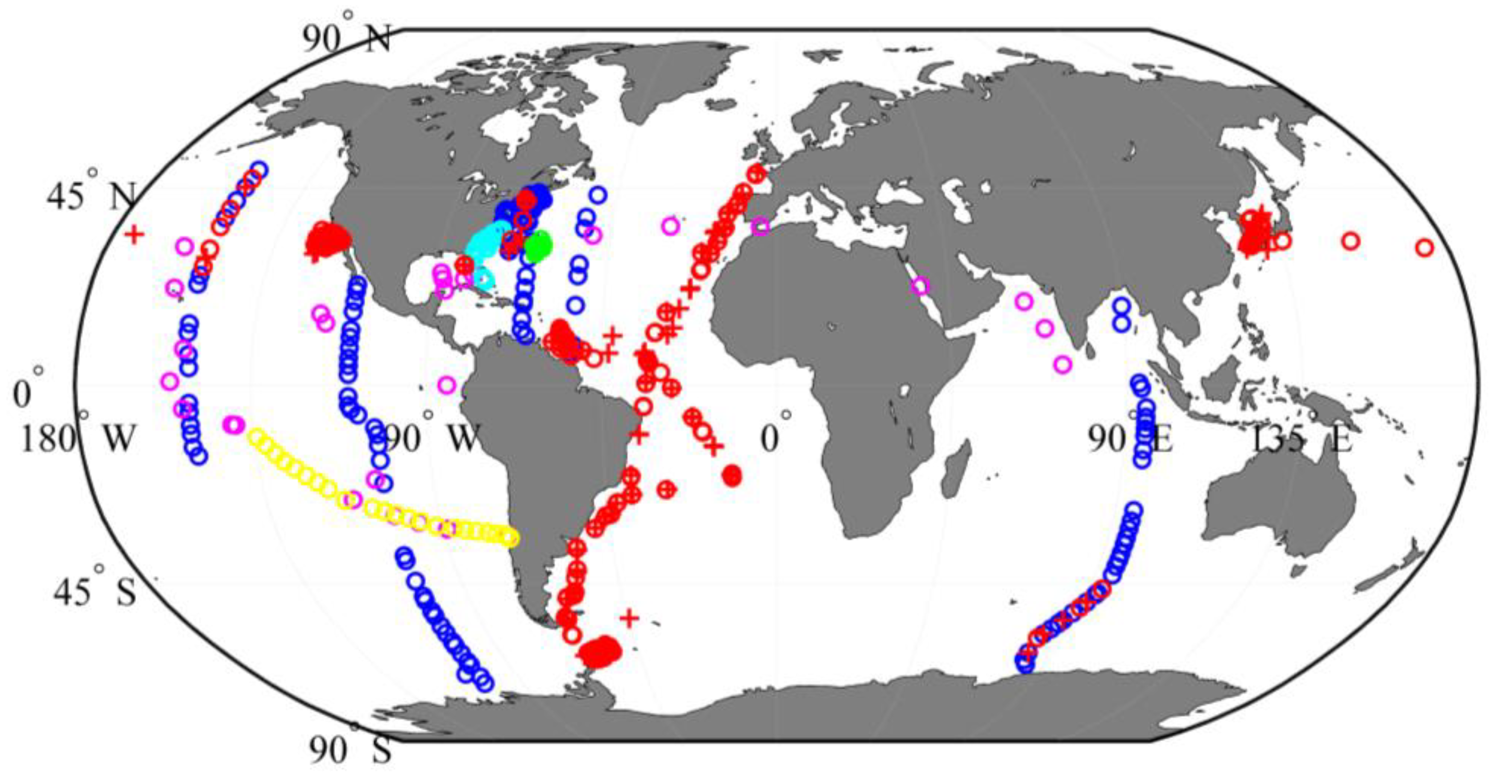
2.1. Datasets and Study Sites

The datasets used in this study can be broadly classified into six different categories: (a) phytoplankton absorption coefficients (a_ph(λ)) from the global oceans; (b) simultaneously collected a_ph(λ) and HPLC; (c) simultaneously measured R_rs(λ), a_ph(λ) and/or HPLC; (d) HPLC time series; (e) R_rs(λ) from MERIS imagery; and (f) HydroLight simulated R_rs(λ), a_ph(λ), particulate backscattering coefficients (b_bp(λ)) and absorption coefficients of colored dissolved and detrital matters (a_dg(λ)) (International Ocean-Color Coordinating Group (IOCCG) dataset [50]).

Table 1. Datasets, time, variables, size and their usages in this study. Cpigs: pigment concentrations, N: the number of samples, NA: not applicable.

Datasets/Cruises	Time	Size (N)	Measurements	Chl-a (mg∙m−3)	Usage
SeaBASS	2001–2012	1619	aph(λ)	NA	Gaussian curves
	1991–2007	430	aph(λ), HPLC	0.02–13.2	aGau(λ) vs. Cpigs relationships
IOCCG	NA	500	Rrs(λ), aph(λ), adg(λ), bbp(λ)	0.03–30	aGau(λ) and Cpigs validation
Tara Oceans expedition	2010–2012	23	Rrs(λ), aph(λ), HPLC	0.02–0.95
VIIRS cal/val	2014–2015	21	Rrs(λ), aph(λ), HPLC	0.15–1.5
BIOSOPE	2004	31	Rrs(λ), aph(λ), HPLC	0.00036–3.06
BATS	2002–2012	148	HPLC	0.002–0.486	Cpigs variation
MERIS	2002–2012	148	Rrs(λ)	0.037–0.325

provides an overview of the different datasets, time, size, variables, [Chl-a] range, and the main usage. The description of each dataset and the data measurements are included in the following paragraphs.

A series of a_ph(λ) spectra measured with the quantitative filter technique (QFT [67]) were used to find the globally optimized Gaussian parameters and the relationships among them. This dataset was obtained by searching the SeaWiFS Bio-optical Archive and Storage System (SeaBASS), which covers 1619 stations across the global oceans observed during 2001–2011. A set of 430 observations that had a_ph(λ) and HPLC measurements coincidently observed were obtained from this dataset and were further randomly separated into two equal subsets (N = 215). The Subset_1 was used for regression analysis between Gaussian peak height (a_Gau(λ)) and pigment concentrations (Cpigs) to obtain the relationships among them; and the Subset_2 together with the a_ph(λ) and HPLC from Tara Oceans, BIOSOPE, and VIIRS cal/val cruises were used to validate the relationships obtained from Subset_1.

The Tara Oceans expedition contains 23 match-ups of R_rs(λ), a_ph(λ) and HPLC around the global ocean. The BIOSOPE dataset includes 31 match-ups of R_rs(λ), a_ph(λ) and HPLC which were collected in the southeastern Pacific Ocean (obtained from: http://www.obs-vlfr.fr/proof/vt/op/ec/biosope/bio.htm). The VIIRS cal/val dataset is composed of 21 R_rs(λ), a_ph(λ) and HPLC measurements obtained from cruises covering the coastal oceans in North Atlantic Ocean off the United States east coast. The BATS (Bermuda Atlantic Time-Series Study) dataset is composed of HPLC time series from 2002 to 2012 and was obtained from the Bermuda Atlantic Time-Series Study (near Bermuda) (http://bats.bios.edu/bats_measurements.html). All of the in situ measurements used are from the surface, defined as a depth ≤5 m. The sampling locations of all these measurements are shown in Figure 1.

The IOCCG dataset was simulated using HydroLight software version 5.1 [68]. It was designed to cover the dynamic range observed across the global ocean but is biased to coastal waters (http://www.ioccg.org/data/synthetic.html). The R_rs(λ), a_ph(λ), a_dg(λ) and b_bp(λ) obtained from this dataset were used to validate the MuPI retrievals.

2.2. Radiometric Measurements

The in situ remote sensing reflectance, R_rs(λ), was calculated based on the measurements of radiance and irradiance sampled with the Radiometer Incorporating the Skylight-Blocked Apparatus (RISBA) [69], Hyper Spectral Radiometer HyperPro free-fall profiler (Satlantic, Inc. Halifax, Nova Scotia, Canada), or above water radiometers [70]. The R_rs(λ) spectra from 350–800 nm with different spectral increments were interpolated to 1 nm resolution.

Standard Level 3 MERIS R_rs(λ) was acquired from the National Aeronautics and Space Administration (NASA) ocean color website (https://oceancolor.gsfc.nasa.gov). The HPLC data from BATS were matched to Level 3 MERIS 8-day products, at 4 km resolution and plus or minus one pixel (3 × 3 window). This criterion, although less restricting than NASA’s 3-h window for data and algorithm validation [71], was adopted to maximize the number of match-ups.

The MuPI model was applied to MERIS R_rs(λ) imagery from 2002–2012 to obtain the seasonal variation of chlorophyll a, b, c, photoprotective and photosynthetic carotenoids concentrations ([Chl-a], [Chl-b], [Chl-c], [PPC], [PSC]) near Bermuda. As examples, global maps of these five different pigments were also obtained from MERIS R_rs(λ) imagery of 2007. The ratios of these concentrations to [Chl-a] are also presented to highlight their independence from chlorophyll a.

2.3. Absorption Measurements

Water samples for absorption and HPLC measurements were filtered onto a GF/F filter and stored in liquid nitrogen before laboratory measurements. Spectrophotometers were used to measure the absorbance and then to calculate the absorption coefficient of particles (a_p) and detrital matter (a_d). The phytoplankton absorption coefficient (a_ph(λ)) were obtained by subtracting a_d from a_p following NASA Ocean Optics Protocols, Revision 4, Volume IV protocol [72]. These a_ph(λ) spectra generally cover 400–800 nm with spectral resolution around 3 nm. They were interpolated into 1 nm resolution for studies here.

Following Hoepffner and Sathyendranath [37,64] and Wang et al. [63,73], the phytoplankton absorption coefficients were decomposed into 13 Gaussian curves using the least square curve fitting technique provided in MATLAB and Statistics Toolbox (Release 2016a, MathWorks, Inc. Natick, MA, USA):

$$a_{\mathrm{ph}}(\lambda )={\displaystyle \sum _{i=1}^n{a}_{\mathrm{Gau}}\left({\lambda }_i\right)\exp \left[-0.5{\left(\frac{\lambda -{\lambda }_i}{{\sigma }_i}\right)}^2\right]}$$

(1)

where σ_i and a_Gau(λ_i) are the width and peak magnitude of the i-th Gaussian curve at peak center (λ_i) as shown in

Table 2. The 12 Gaussian curves corresponding to the phytoplankton pigment absorption coefficients, with Peak_loc as the center location of each pigment absorption peak and width as the full width at half maximum (FWHM). The relationships indicate the power-law relationships used to estimate the Gaussian peak amplitudes from the two independent variables: x₁: a_Gau(434) and x₂: a_Gau(492). Chl-a: chlorophyll a, Chl-b: chlorophyll b, Chl-c: chlorophyll c, PPC: photo-protective carotenoids, PSC: photosynthetic carotenoids, PE: phycoerythrin and PC: phycocyanin.

Peak	Pigments	Peak_loc (nm)	Width(FWHM) (nm)	Relationships	R2
1	Chl-a	406	16	1.13x11.01	0.98
2	Chl-a	434	12	x1	--
3	Chl-c	453	12	0.60x10.95	0.99
4	Chl-b	470	13	0.51x10.97	0.98
5	PPC	492	16	x2	--
6	PSC	523	14	0.87x21.17	0.99
7	PE	550	14	0.79x21.27	0.96
8	Chl-c	584	16	0.40x21.17	0.96
9	PC	617	13	0.34x11.14	0.93
10	Chl-c	638	11	0.47x21.19	0.96
11	Chl-b	660	11	0.30x21.11	0.94
12	Chl-a	675	10	0.86x11.11	0.98

. The obtained a_Gau(λ) are used as ground truth to validate the inversion results from R_rs(λ).

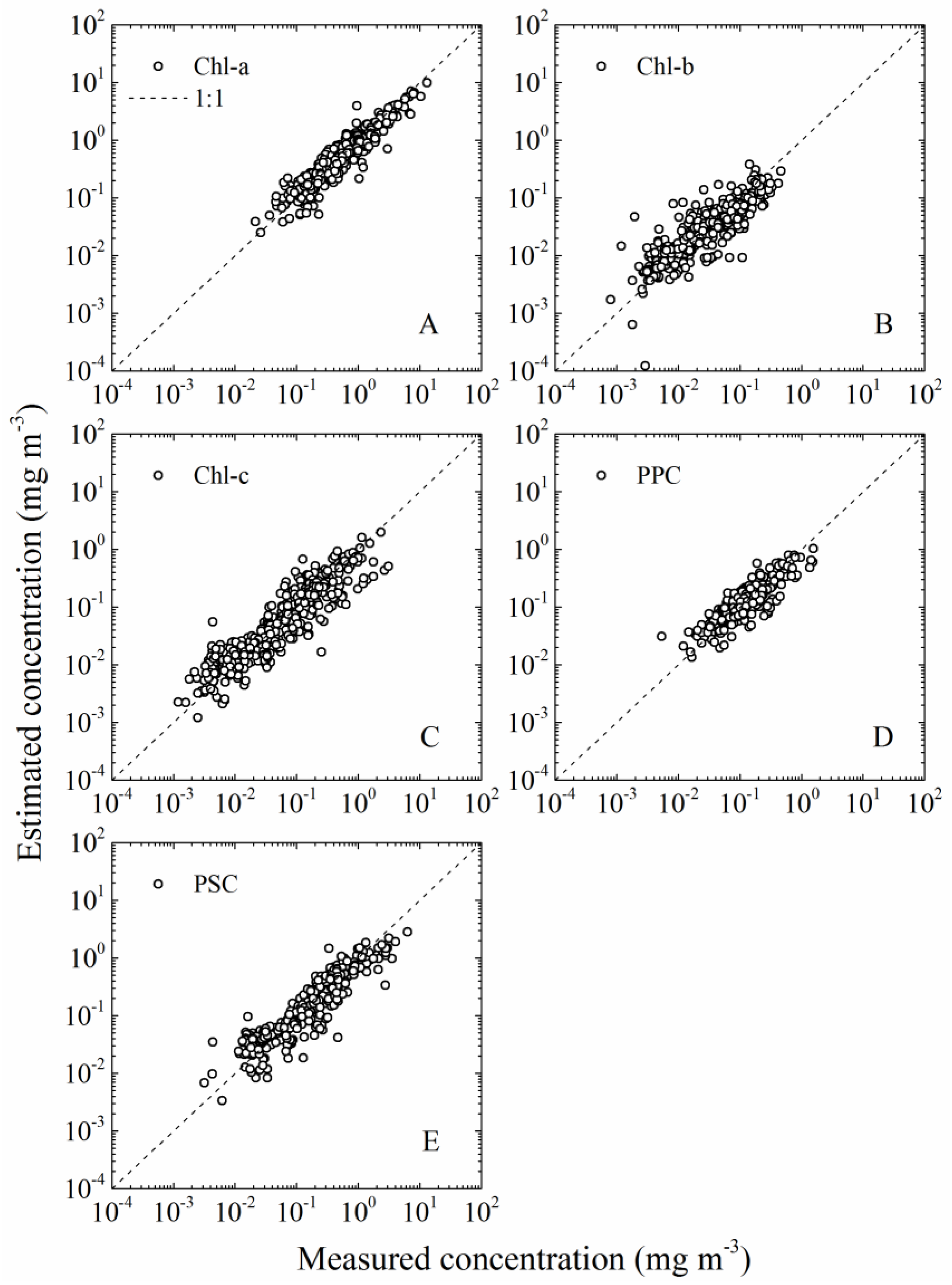
2.4. Pigment Concentrations

All the HPLC analyses were carried out according to the method following or adapted from Van Heukelem and Thomas [23]. The concentrations of chlorophyll a, b, c, photo-protective carotenoids (PPC) and photosynthetic carotenoids (PSC) were estimated from HPLC measurements as:

(A)

Total chlorophyll a (Chl-a) = chlorophyll a + divinyl chlorophyll a + chlorophyllide a;

(B)

Total chlorophyll b (Chl-b) = chlorophyll b + divinyl chlorophyll b;

(C)

chlorophyll c (Chl-c) = chlorophyll c1 + chlorophyll c2;

(D)

PPC = α-carotene + β-carotene + zeaxanthin + alloxanthin + diadinoxanthin;

(E)

PSC = 19′-hexanoyloxyfucoxanthin + fucoxanthin + 19′-butanoyloxyfucoxanthin + peridinin.

MERIS [Chl-a] was estimated from the Level 3 R_rs(λ) following the standard algorithm OC4E provided by NASA [4]. Details about this algorithm can be found on the following webpage: https://oceancolor.gsfc.nasa.gov/atbd/chlor_a/.

2.5. Pigment Retrieval from R_rs(λ)

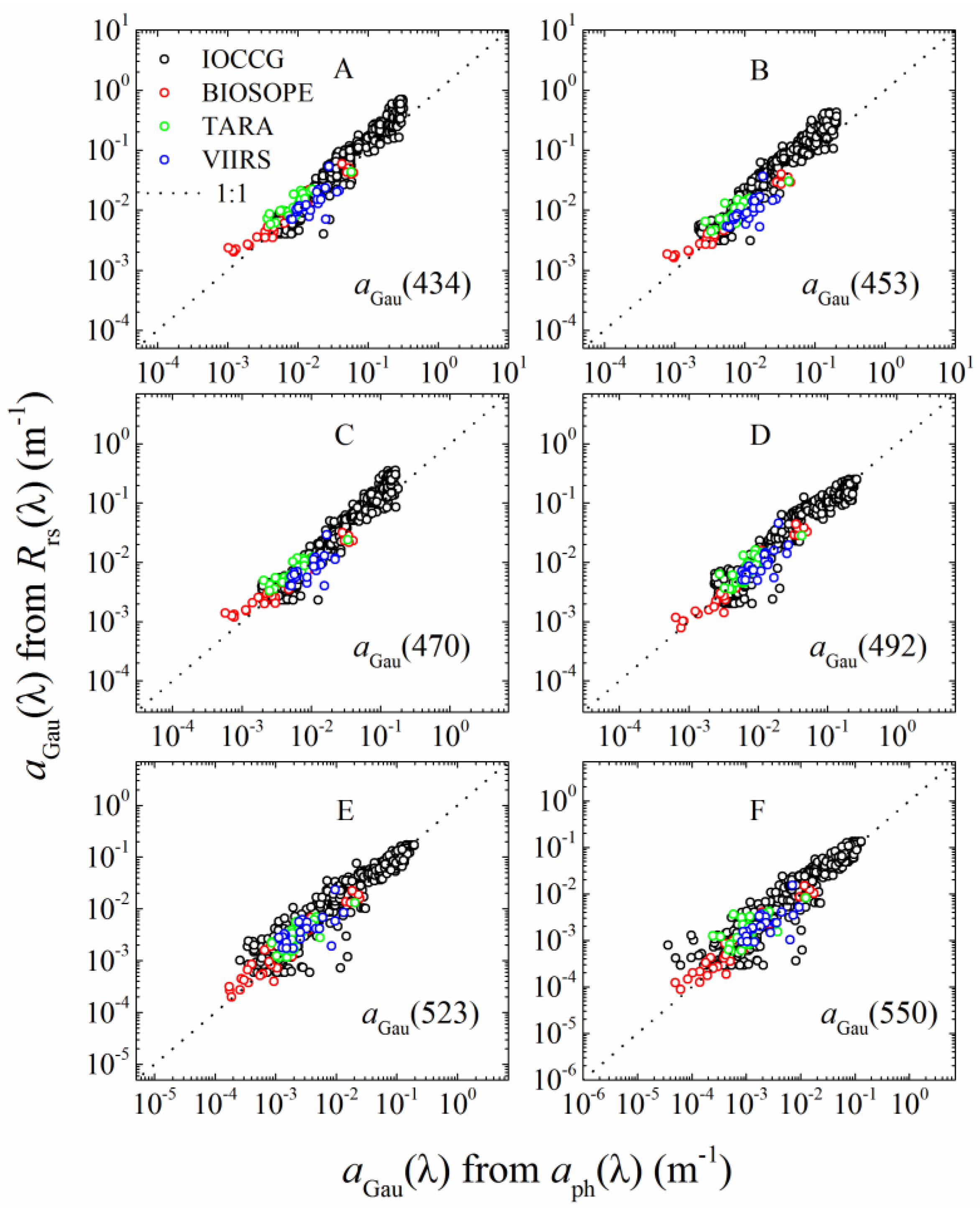
2.5.1. a_Gau(λ) from R_rs(λ)

The multi-pigment inversion model (MuPI) was used to retrieve a_Gau(λ) from R_rs(λ). Wang et al. [63,73] developed this semi-analytical inversion model (MuPI) to retrieve a_Gau(λ) from hyper- or multi-spectral R_rs(λ). A brief description of MuPI is presented here. The functional relationship between R_rs(λ) and inherent optical properties (IOPs) is taken from Gordon et al. [47] and Lee et al. [49]:

$$R_{\mathrm{rs}}\left(\lambda \right)=0.52{\displaystyle \sum _{i=1}^2{g}_i}{\left[\frac{b_{\mathrm{b}}\left(\lambda \right)}{a\left(\lambda \right)+b_{\mathrm{b}}\left(\lambda \right)}\right]}^i/\left\{1-1.7{\displaystyle \sum _{i=1}^2{g}_i}{\left[\frac{b_{\mathrm{b}}\left(\lambda \right)}{a\left(\lambda \right)+b_{\mathrm{b}}\left(\lambda \right)}\right]}^i\right\}$$

(2)

where g₁ (sr⁻¹) and g₂ (sr⁻¹) are fixed to 0.089 and 0.125 sr⁻¹. The IOP spectra, a(λ) and b_b(λ), are partitioned into relevant components

$$b_{\mathrm{b}}\left(\lambda \right)=b_{\mathrm{bw}}\left(\lambda \right)+b_{\mathrm{bp}}\left(\lambda \right)$$

(3)

$$a\left(\lambda \right)=a_{\mathrm{w}}\left(\lambda \right)+a_{\mathrm{ph}}\left(\lambda \right)+a_{\mathrm{dg}}\left(\lambda \right)$$

(4)

with b_bw(λ) for seawater backscattering coefficient [74] and a_w(λ) for seawater absorption coefficient [75,76]. Phytoplankton absorption coefficient (a_ph(λ)) is modeled following Equation (1); b_bp(λ), particulate backscattering coefficient, is modeled following Equations (5) and (6) [49]; and the combined dissolved and detrital particulate absorption coefficient a_dg(λ) is modeled using Equation (7) [52,77,78].

$$b_{\mathrm{bp}}=b_{\mathrm{bp}}({\lambda }_0){\left(\frac{{\lambda }_0}{\lambda }\right)}^{\eta }$$

(5)

$$\eta =2\left(1-1.2\exp \left(-0.9\frac{R_{\mathrm{rs}}(440)}{R_{\mathrm{rs}}(550)}\right)\right)$$

(6)

$$a_{\mathrm{dg}}\left(\lambda \right)=a_{\mathrm{dg}}\left({\lambda }_0\right)\exp \left(-S\left(\lambda -{\lambda }_0\right)\right)$$

(7)

where λ₀ is a reference wavelength (nearest to 440 nm), S is the spectral decay constant for absorption of detrital and dissolved materials and kept as an unknown within 0.007 to 0.02 nm⁻¹ [52,77,78]. η is the power-law exponent for the particulate backscattering coefficient calculated from the R_rs(440) to R_rs(550) ratio following Lee et al. [49].

In the determination of Gaussian parameters (σ_i and λ_i) for a_ph(λ) in the global scale, we also tested various combinations of parameters using data published in the literature [63,64,65]. The existing parameters were not successful at obtaining satisfactory results for every data range due to various reasons, including the fact that the initial datasets used to obtain the parameters had a small dynamic range unable to cover varied conditions such as coastal regions and non-bloom natural oceanic waters. Thus, a refinement of the parameters σ_i and λ_i was conducted using the a_ph(λ) dataset obtained from SeaBASS to improve the overall performance of the MuPI model for global oceans. The non-linear least square fitting procedure in MATLAB was used to solve Equation (1). A set of refined Gaussian parameters for σ_i and λ_i were obtained and are presented in Table 2. For oceanic waters, as the absorption coefficient from water molecules contributes >80% of the total absorption coefficient for wavelengths >550 nm, it is difficult to obtain accurate a_Gau(λ) by directly inverting R_rs(λ) in the longer wavelengths. On the other hand, since the Gaussian peaks at 434 and 492 nm cover the main absorption features of the different pigments, the two a_Gau(λ) at 434 and 492 nm were chosen as the independent variables in this effort.

Following Wang et al. [73], the implementation of this model used two Gaussian peak heights [a_Gau(λ₁) and a_Gau(λ₂)] to reconstruct a_ph(λ), in which empirical relationships as shown in Table 2 were used. These relationships between a_Gau(λ) were obtained by regression analysis with the purpose of reducing the unknowns in the R_rs(λ) inversion procedure [63,73]. With this design, there will be five unknowns [a_Gau(λ₁), a_Gau(λ₂), b_bp(λ₀), a_dg(λ₀) and S] to be retrieved from a R_rs(λ) spectrum, which is obtained by a minimization of the cost function (Equation (8)):

$$\delta =\frac{\sqrt{\frac{1}{N_{\lambda }}{\displaystyle \sum _{i=1}^{N_{\lambda }}{\left({\widehat{R}}_{\mathrm{rs}}\left({\lambda }_i\right)-R_{\mathrm{rs}}\left({\lambda }_i\right)\right)}^2}}}{\frac{1}{N_{\lambda }}{\displaystyle \sum _{i=1}^{N_{\lambda }}{R}_{\mathrm{rs}}\left({\lambda }_i\right)}}$$

(8)

with N_λ as the wavelength number, R_rs(λ) as the measured, and Ȓ_rs(λ) the modeled spectrum, respectively. Basically, δ value provides a measure of the relative difference between the input and output R_rs spectra. The generalized reduced gradient (GRG) nonlinear optimization procedure [79] was used to solve Equation (8).

The statistical indices used to estimate the agreement between the two values (Ȓ and R) was the unbiased absolute percentage difference (UAPD), defined as Equation (9) and root mean square error (RMSE, Equation (10)) with N as the number of samples.

$$\mathrm{UAPD}=\frac{\left|\widehat{R}-R\right|}{0.5\left(\widehat{R}+R\right)}\times 100\%$$

(9)

$$\mathrm{RMSE}=\sqrt{\frac{1}{N}{\left(\widehat{R}-R\right)}^2}$$

(10)

2.5.2. a_Gau(λ) Versus Cpigs

Hoepffner and Sathyendranath [64] indicated that each Gaussian curve represents the absorption contributed by one or multiple pigments. However, attempts to obtain the concentration of a specific pigment from a single Gaussian curve is not always successful [39,65,66]. For a better understanding of the Gaussian curves and their relationships with Cpigs, a series of regression analyses were applied to relate a_Gau(λ) with Cpigs for data from SeaBASS. The t-statistics and p-value were calculated to test the significance of the parameters. Using p < 0.05 as the criteria, the significant contributors to each Gaussian peak and the corresponding R² of these parameters were obtained (see

Table 3. The p-value and R² from the t-statistics, with a_Gau(λ) at 12 different wavelengths: 406, 434, 453, 470, 492, 523, 550, 584, 617, 638, 660, and 675 nm, and Chl-a: chlorophyll a, Chl-b: chlorophyll b, Chl-c: chlorophyll c, PPC: photo-protective carotenoids, PSC: photosynthetic carotenoids.

p-Value	Peak 406	Peak 434	Peak 453	Peak 470	Peak 492	Peak 523	Peak 550	Peak 584	Peak 617	Peak 638	Peak 660	Peak 675
Chl-a	0.01	0.00	0.00			0.01	0.03	0.00	0.00	0.00	0.00	0.00
Chl-b		0.03		0.00
Chl-c							0.04	0.03			0.00	0.04
PPC	0.00		0.00	0.00	0.00
PSC				0.00	0.02	0.01
R2	0.80	0.87	0.83	0.87	0.83	0.78	0.64	0.68	0.76	0.73	0.81	0.91

). The possible existence of other pigments that are not detectable with current HPLC techniques, such as phycoerythrin (PE) and phycocyanin (PC), likely explains the relatively lower R² values for Peaks 7, 8, 9 and 10.

After a series of multivariable regression analyses, it was found that Cpigs could be estimated from a_Gau(λ) following the function:

$${\log }_{10}\left(\mathrm{Cpigs}\right)=a_0+{\displaystyle \sum _{i=1}^n{a}_i{\log }_{10}\left(a_{\mathrm{Gau}}({\lambda }_i)\right)}$$

(11)

The corresponding a_Gau(λ), parameters, and the R² value are shown in

Table 4. Parameters for estimation of pigment concentrations: the pigment-specific a_Gau(λ), coefficients and R². Chl-a: chlorophyll a, Chl-b: chlorophyll b, Chl-c: chlorophyll c, PPC: photo-protective carotenoids, PSC: photosynthetic carotenoids.

Pigments	aGau(λ)	Parameters (a0, a1, …, ai)	R2
Chl-a	675	1.804, 0.975	0.89
Chl-b	434, 453, 470	−0.066, 2.470, −3.073, 1.379	0.72
Chl-c	470, 492, 523, 675	1.334, 2.022, −3.125, 0.745, 1.119	0.83
PPC	453, 470	0.734, 1.311, −0.416	0.76
PSC	470, 492, 523	1.67, 3.034, −2.670, 0.725	0.84

. Further, it was found that the estimated Cpigs agree with the measured values very well throughout the concentration range when the relationships were applied to the validation dataset (with data points scattered closely to the 1:1 line; Figure 2).

3. Results

3.1. Retrievals from R_rs(λ)

3.1.1. a_Gau(λ) Validation

The MuPI model was first tested with datasets that contained different levels of chlorophyll a concentration from the IOCCG synthesized data and different cruises in the global ocean. The main purpose of this test was to evaluate, and validate, the implementation of the MuPI approach for a wide range of environments. A mean UAPD of 36% was obtained between a_Gau(λ) from R_rs(λ) inversion and a_Gau(λ) from water samples throughout the data range for different datasets (see Figure 3). The differences in statistical results, noted in

Table 5. Mean (Mea.) and median (Med.) of the unbiased percentage errors for a_Gau(λ) retrieval from R_rs(λ) for different datasets.

Peak Center	IOCCG		Tara Oceans		BIOSOPE		VIIRS Cruises
	Mea.	Med.	Mea.	Med.	Mea.	Med.	Mea.	Med.
406	45	45	34	27	34	28	28	20
434	37	36	34	28	26	25	28	13
453	47	49	28	24	23	18	27	15
470	35	34	29	25	30	27	31	18
492	34	31	26	21	22	18	29	18
523	44	34	38	28	34	29	48	44
550	45	35	53	41	37	34	41	35
584	55	48	48	37	38	36	53	57
617	51	45	47	38	36	29	37	40
638	54	42	66	68	41	35	41	35
660	52	48	35	23	32	29	43	34
675	46	40	30	26	60	56	32	21

for a_Gau(λ) retrieval from different datasets, are strongly influenced by their different dynamic ranges and characteristics as implied in Section 2.1.

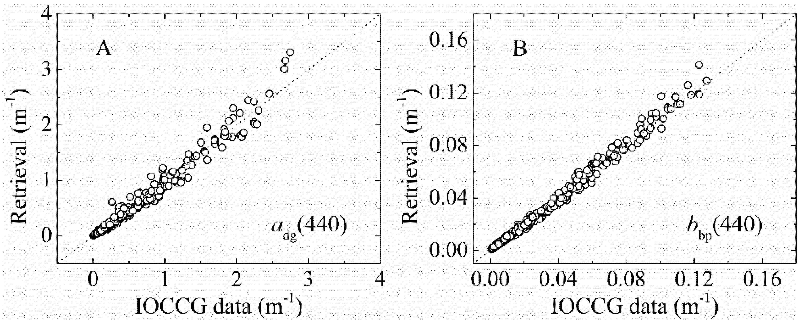
3.1.2. b_bp(λ) and a_dg(λ) Validation

The backscattering coefficients of particles and absorption coefficients of detrital and dissolved materials retrieved from R_rs(λ) by MuPI have also been validated with the IOCCG dataset (with values at 440 nm as examples). The b_bp(440) showed very high accuracy with mean UAPD of 4.8%, and all samples showed no bias in the entire data range as presented in Figure 4A. The estimated a_dg(440) also showed very good agreement with the simulated values, with the mean UAPD of 21.3%. No inter-comparisons were made for the products a_dg(λ) and b_bp(λ) for other datasets because of lacking corresponding measured data.

3.2. Cpigs from Satellite Remote Sensing

3.2.1. Cpigs Validation and Their Seasonal Variation

The ability of MuPI to capture the magnitudes of Cpigs and their seasonal variability from satellite R_rs(λ) was then validated using a time series of HPLC measurements at BATS from the years 2002 to 2012. During this period of time, Cpigs varied in these ranges: [Chl-a]: 0.016–0.486 mg∙m⁻³, [Chl-b]: 0.001–0.108 mg∙m⁻³, [Chl-c]: 0.001–0.206 mg∙m⁻³, [PPC]: 0.004–0.147 mg∙m⁻³, and [PSC]: 0.003–0.106 mg∙m⁻³.

To obtain Cpigs from satellite R_rs(λ), a_Gau(λ) were inverted first from R_rs(λ) using MuPI, then Equation (11) was applied to convert the retrieved a_Gau(λ) to Cpigs. As shown in Figure 5, it is found that there are good matches in the magnitudes and the seasonal cycles for the five pigments, with mean UAPD values as 38%, 78%, 65%, 36%, and 47% (and the medians are 34%, 79%, 64%, 30% and 55%) for [Chl-a], [Chl-b], [Chl-c], [PPC] and [PSC], respectively. The [Chl-a] accuracy is comparable with the NASA adopted standard [Chl-a] algorithms, for which the color index (CI) algorithm [5] showed a mean UAPD of 38.6% and OC4E of 46.7%. There are many reasons for the relatively low accuracy in the retrieval of [Chl-b] and [Chl-c], which include very low concentrations (e.g., in situ [Chl-b] and [Chl-c] were close to the HPLC detection minimum), as well as uncertainties in satellite measured R_rs(λ), and the derived a_Gau(λ) from R_rs(λ).

Beyond the seasonal cycles in Cpig magnitudes, variation in pigment composition over time implied in the change of pigment ratios was also noticed in Figure 6A. On further examination, we found the ratios derived from MERIS R_rs(λ) using MuPI can pick up the variation in the [Chl-b], [Chl-c], [PPC], [PSC] to [Chl-a] ratios observed from HPLC measurements very well with the mean UAPD of 50%, 47%, 25%, 37%, and median of 38%, 39%, 19% and 29% respectively (Figure 6B). Since these phytoplankton pigment ratios do not co-vary with the [Chl-a] product and cannot be empirically estimated from [Chl-a] alone, the Gaussian peaks and multiple pigments retrieved here provide a valuable glimpse into potential applications of these ratios in ocean changes that can be studied at large spatial and high temporal scales.

3.2.2. Global Distribution of Cpigs

As an example, MuPI was applied to MERIS L3 global annual (2007) average R_rs(λ) to obtain the global distribution of the five different pigment concentrations (Figure 7 and Figure 8) and their ratios to [Chl-a] (Figure 9). The global patterns of [Chl-a], [Chl-b], [Chl-c], [PPC], and [PSC] mimic the major gyre systems and other large-scale circulation features of the world ocean. High values of Cpigs are found within regions of persistent large-scale upwelling (e.g., subarctic gyres, equatorial divergences, eastern boundary currents, etc.), while low values are observed where large-scale downwelling is observed (e.g., subtropical gyres).

The basin-scale [Chl-a] distribution follows the pattern reported in the literature [4,5]. In comparing the global map of [Chl-a] derived in this study with the standard product from NASA ocean color website (Figure 7), some differences were noticed. In the previous section, when using HPLC data from BATS for validation, the retrieved [Chl-a] showed higher accuracy via MuPI than that from the standard OC4E algorithm. To better understand the differences in [Chl-a] distribution at the global scale, a validation dataset from SeaBASS was used. This dataset was obtained by searching match-ups of in situ measured [Chl-a] with those from MERIS R_rs(λ). A dataset containing 608 pairs of [Chl-a] and MERIS R_rs(λ) were obtained in which [Chl-a] concentrations ranged from ~0.017 to ~40.3 mg∙m⁻³ (locations shown in Figure 7A). In comparing the estimated [Chl-a] from two different methods with in situ measurements (Figure 7C), MuPI and OC4E showed comparable results with mean UAPD of 48.8% and RMSE of 4.51 mg∙m⁻³ for OC4E and mean UAPD of 49.3% and RMSE of 4.05 mg∙m⁻³ for MuPI. As shown in Figure 7C, the [Chl-a] estimated from OC4E is biased slightly high (~10%) in the range of 1–10 mg∙m⁻³ compared with results from MuPI. This range of [Chl-a] (1–10 mg∙m⁻³) is mainly from coastal and inland waters for which the influences from colored dissolved and detrital matter result in lower accuracy in band-ratio estimated [Chl-a] [80]. For several samples, the [Chl-a] values from MuPI are biased low (~70%) as shown in Figure 7C. There are two possible reasons for this: (1) bad input MERIS R_rs(λ), not only the values but also the spectral shape, especially at the blue bands that are susceptible to poor atmospheric correction, where negative values are often observed for coastal waters [81]; (2) the limitation of the algorithm as a result of the empirical parameters used to reduce the unknowns in MuPI, and the low contribution of a_ph(λ) to the total absorption coefficients in the 400–750 nm range, which will be further discussed in Section 4.

The pigment ratios to [Chl-a] showed complicated patterns (Figure 9). In high [Chl-a] regions, [Chl-b]/[Chl-a] and [PPC]/[Chl-a] are low. In some low [Chl-a] regions, the ratios of [Chl-c]/[Chl-a] and [PSC]/[Chl-a] are relatively high, such as in the East Pacific Ocean. These results agree with previous findings about the global distribution of phytoplankton groups and pigment ratios, as lower [PPC]/[Chl-a] ratios correspond to high [Chl-a] and larger particle size [9,17,82,83,84]. As recorded in the literature, in different regions of the global ocean, the quality and quantity of light and nutrient, as well as temperature, is highly variable [85]. These highly unpredictable and rapid changes of the environment usually result in phytoplankton taxonomic composition variation (long-term adaptation) or physiological acclimation (short-term acclimation) [24]. The variation in pigment ratios obtained from MuPI can directly reflect these changes in phytoplankton and provide valuable information for phytoplankton studies in large spatial and high temporal scales.

4. Discussion

Based on the initial model of Wang et al. [63] that was developed for bloom waters, we have demonstrated that using a set of refined parameters for the Gaussian curves for global waters (Table 2), the MuPI model demonstrates consistent performance in a_Gau(λ) retrievals on a global scale, as shown in Figure 3 and Figure 4 and Table 5. Compared with HPLC measurements, the estimates of [Chl-a], [Chl-b], [Chl-c], [PPC] and [PSC] from satellite R_rs(λ) showed reasonable accuracies, with the mean UAPD of 38%, 78%, 65%, 36%, and 47% respectively (Figure 5). Further, the distribution of these pigments and their ratios to [Chl-a], were obtained from MERIS measurements on the global scale (Figure 8 and Figure 9).

The phytoplankton pigment ratios are critical indicators of the variation in phytoplankton groups and species due to their physiological adaptation to changes in nutrients, temperature, and light availability over time and space. The HPLC measured pigment concentrations and ratios have been widely used for determining the phytoplankton taxonomic composition and estimating the biomass of different groups, such as in CHEMTAX [27] and PFT analyses [10]. However, lacking effective methods, the estimation of phytoplankton pigments from satellite remote sensing has been limited to only [Chl-a] in the past decades [3,4,5], and the efforts made to obtain the accessory pigments have been more or less based on empirical relationships with Chl-a [45,46]. Thus, these products provided limited ability to capture the variation in the physiological status of phytoplankton. However, these unknown physiological variations in phytoplankton pigments have been one of the main uncertainties in traditional phytoplankton remote sensing models that use [Chl-a] as input to represent the phytoplankton biomass, such as the traditional [Chl-a] based primary productivity [14,20]. MuPI, as shown in this study, fills in this gap by obtaining not only the accessory pigment concentrations but also their ratios to [Chl-a] on the global scale, and reasonable accuracy has been obtained in validation with in situ data.

[Chl-a] is by far the easiest quantity to validate as it is routinely measured. An independent evaluation of the model has been conducted with the MERIS match-up dataset (Figure 7). This dataset contains nearly simultaneous in situ [Chl-a] measurements and MERIS R_rs(λ) at coincident locations. To evaluate other pigments, an independent evaluation was conducted with MERIS R_rs(λ) and in situ HPLC match-ups from 2002 to 2012 near Bermuda (Figure 5). The match-up dataset contains data from different seasons over a decadal scale. Use of the model with the match-up dataset from BATS confirms good overall behavior of the MuPI model for pigment concentration and pigment ratio retrievals, demonstrating the ability of the model to obtain accurate information from satellite ocean color imagery. However, because of the limitation of in situ pigment concentrations, the potential of obtaining PE and PC concentrations from satellite remote sensing data was not addressed in this study.

The main difficulty in making the model more applicable with any waterbody comes from the parameterization of the Gaussian curves, particularly the empirical relationships among a_Gau(λ). Although it is reasonably straightforward to optimize the parameters with each dataset to obtain better retrievals, it would be extremely difficult (if not impossible) to do so when in situ measurements from the target location are hard to obtain. Instead, a set of globally optimized parameters were obtained using a dataset that covers a large dynamic range of the global ocean. Another challenge for a_Gau(λ) retrieval in the open ocean lies in the low contribution of pigment absorption to the total absorption coefficient around 550–650 nm. Thus, it is difficult to directly invert R_rs(λ) to obtain pigment absorption coefficients at the longer wavelengths (>550 nm).

This version of the MuPI model should be considered interim because the model could be further updated when more global data become available. In its present form, the model is optimized to work with R_rs(λ) data from the first nine MERIS bands. As a first step, several components of the Gaussian model were deliberately formulated by use of empirical relationships to limit the number of unknowns to be solved via the spectral optimization procedure. This is particularly true for estimation of 13 a_Gau(λ) from two independent Gaussian curves, which significantly reduced the unknowns. Instead of the Gaussian scheme, another potential way to obtain different pigment information from remote sensing data is through the specific absorption coefficients as adopted by many studies [46,86]. However, the specific absorption coefficients have significant limitations, such as the variation of the coefficients in different waters and the lack of routine measurements of some pigments, such as PE and PC [46,86,87].

With the information of accessory pigments obtained from MuPI, different biogeochemical studies could be conducted: 1. Remotely sensed PE and PC concentrations could be validated and applied to the estimation of cyanobacteria on a global scale. 2. The pigment ratios could be used as a direct indicator for estimation of phytoplankton functional types or functional traits, and phytoplankton physiological variation over space and time. 3. The pigment absorption coefficients (photoprotective and photosynthetic) could be estimated from satellite remote sensing data and incorporated into models for more accurate estimation of primary productivity.

5. Conclusions

The multi-pigment inversion model, namely MuPI, which semi-analytically obtains concentrations of multiple pigments from remote sensing reflectance, has been validated and applied to MERIS R_rs(λ) imagery to obtain not only [Chl-a], but also [Chl-b], [Chl-c], [PPC], [PSC] (and subsequently their ratios to [Chl-a]) in the global oceans. The obtained pigment concentrations and the pigment ratios showed good agreement with in situ HPLC data, with the mean UAPD of 38%, 78%, 65%, 36%, and 47% respectively. Further, at the global scale, the MuPI obtained [Chl-a] from MERIS showed comparable results with those estimated from the widely used OC4E algorithm with mean UAPD of 48.8% and RMSE of 4.51 mg∙m⁻³ for OC4E and mean UAPD of 49.3% and RMSE of 4.05 mg∙m⁻³ for MuPI. However, unlike OC4E, MuPI as a semi-analytical model provided reasonable retrievals of several parameters {[Chl-a], [Chl-b], [Chl-c], [PPC], [PSC], a_dg(440) and b_bp(440)} simultaneously from satellite obtained remote sensing reflectance. The information of these accessory pigments would extend the application of satellite ocean color data in global biogeochemical studies that was previously limited due to [Chl-a] as the only available pigment.

References

1. Falkowski, P.G. The role of phytoplankton photosynthesis in global biogeochemical cycles. Photosynth. Res. 1994, 39, 235–258. [Google Scholar] [CrossRef] [PubMed] [Green Version]
2. Kiørboe, T. Turbulence, phytoplankton cell size, and the structure of pelagic food webs. In Advances in Marine Biology; Academic Press: Cambridge, MA, USA, 1993; Volume 29, pp. 1–72. [Google Scholar]
3. Gordon, H.R.; Clark, D.K.; Brown, J.W.; Brown, O.B.; Evans, R.H.; Broenkow, W.W. Phytoplankton pigment concentrations in the Middle Atlantic Bight: Comparison of ship determinations and CZCS estimates. Appl. Opt. 1983, 22, 20–36. [Google Scholar] [CrossRef] [PubMed]
4. O’Reilly, J.E.S.; Maritorena, B.G.; Mitchell, D.A.; Siegel, K.L.; Carder, S.A.; Garver, M.; Kahru, C.R. McClain, Ocean color chlorophyll algorithms for SeaWiFS. J. Geophys. Res. 1998, 103, 24937–24953. [Google Scholar] [CrossRef]
5. Hu, C.; Lee, Z.; Franz, B. Chlorophyll algorithms for oligotrophic oceans: A novel approach based on three-band reflectance difference. J. Geophys. Res. 2012, 117. [Google Scholar] [CrossRef]
6. Alvain, S.; Moulin, C.; Dandonneau, Y.; Bréon, F.M. Remote sensing of phytoplankton groups in case 1 waters from global SeaWiFS imagery. Deep Sea Res. Part I Oceanogr. Res. Pap. 2005, 52, 1989–2004. [Google Scholar] [CrossRef] [Green Version]
7. Bracher, A.; Vountas, M.; Dinter, T.; Burrows, J.P.; Röttgers, R.; Peeken, I. Quantitative observation of cyanobacteria and diatoms from space using PhytoDOAS on SCIAMACHY data. Biogeosciences 2009, 6, 751–764. [Google Scholar] [CrossRef] [Green Version]
8. Ciotti, A.M.; Bricaud, A. Retrievals of a size parameter for phytoplankton and spectral light absorption by colored detrital matter from water-leaving radiances at SeaWiFS channels in a continental shelf region off Brazil. Limnol. Oceanogr. Methods 2006, 4, 237–253. [Google Scholar] [CrossRef] [Green Version]
9. Brewin, R.J.; Sathyendranath, S.; Hirata, T.; Lavender, S.J.; Barciela, R.M.; Hardman-Mountford, N.J. A three-component model of phytoplankton size class for the Atlantic Ocean. Ecol. Model. 2010, 221, 1472–1483. [Google Scholar] [CrossRef]
10. Hirata, T.; Hardman-Mountford, N.J.; Brewin, R.J.W.; Aiken, J.; Barlow, R.; Suzuki, K.; Yamanaka, Y. Synoptic relationships between surface Chlorophyll-a and diagnostic pigments specific to phytoplankton functional types. Biogeosciences 2011, 8, 311–327. [Google Scholar] [CrossRef] [Green Version]
11. Mouw, C.B.; Yoder, J.A. Optical determination of phytoplankton size composition from global SeaWiFS imagery. J. Geophys. Res. Oceans 2010, 115. [Google Scholar] [CrossRef] [Green Version]
12. Sathyendranath, S.; Cota, G.; Stuart, V.; Maass, H.; Platt, T. Remote sensing of phytoplankton pigments: A comparison of empirical and theoretical approaches. Int. J. Remote Sens. 2001, 22, 249–273. [Google Scholar] [CrossRef]
13. Gitelson, A.A.; Schalles, J.F.; Hladik, C.M. Remote chlorophyll-a retrieval in turbid, productive estuaries: Chesapeake Bay case study. Remote Sens. Environ. 2007, 109, 464–472. [Google Scholar] [CrossRef]
14. Behrenfeld, M.J.; Falkowski, P.G. Photosynthetic rates derived from satellite-based chlorophyll concentration. Limnol. Oceanogr. 1997, 42, 1–20. [Google Scholar] [CrossRef] [Green Version]
15. Stumpf, R.P.; Culver, M.E.; Tester, P.A.; Tomlinson, M.; Kirkpatrick, G.J.; Pederson, B.A.; Soracco, M. Monitoring Karenia brevis blooms in the Gulf of Mexico using satellite ocean color imagery and other data. Harmful Algae 2003, 2, 147–160. [Google Scholar] [CrossRef]
16. Lehman, P.W. Comparison of chlorophyll a and carotenoid pigments as predictors of phytoplankton biomass. Mar. Biol. 1981, 65, 237–244. [Google Scholar] [CrossRef]
17. Schitüter, L.; Riemann, B.; Søndergaard, M. Nutrient limitation in relation to phytoplankton carotenoid/chlorophyll a ratios in freshwater mesocosms. J. Plankton Res. 1997, 19, 891–906. [Google Scholar] [CrossRef]
18. Breton, E.; Brunet, C.; Sautour, B.; Brylinski, J.M. Annual variations of phytoplankton biomass in the Eastern English Channel: Comparison by pigment signatures and microscopic counts. J. Plankton Res. 2000, 22, 1423–1440. [Google Scholar] [CrossRef]
19. Kruskopf, M.; Flynn, K.J. Chlorophyll content and fluorescence responses cannot be used to gauge reliably phytoplankton biomass, nutrient status or growth rate. New Phytol. 2006, 169, 525–536. [Google Scholar] [CrossRef] [PubMed]
20. Behrenfeld, M.J.; O’Malley, R.T.; Boss, E.S.; Westberry, T.K.; Graff, J.R.; Halsey, K.H.; Brown, M.B. Revaluating ocean warming impacts on global phytoplankton. Nat. Clim. Chang. 2016, 6, 323. [Google Scholar] [CrossRef]
21. Bidigare, R.R.; Morrow, J.H.; Kiefer, D.A. Derivative analysis of spectral absorption by photosynthetic pigments in the western Sargasso Sea. J. Mar. Res. 1989, 47, 323–341. [Google Scholar] [CrossRef]
22. Jeffrey, S.W.; Vesk, M. Introduction to marine phytoplankton and their pigment signature. In Phytoplankton Pigments in Oceanography; UNESCO Publishing: Paris, France, 1997; p. 3784. [Google Scholar]
23. Kirkpatrick, G.J.; Millie, D.F.; Moline, M.A.; Schofield, O. Optical discrimination of a phytoplankton species in natural mixed populations. Limnol. Oceanogr. 2000, 45, 467–471. [Google Scholar] [CrossRef] [Green Version]
24. Van Heukelem, L.; Thomas, C.S. Computer-assisted high-performance liquid chromatography method development with applications to the isolation and analysis of phytoplankton pigments. J. Chromatogr. A 2001, 910, 31–49. [Google Scholar] [CrossRef]
25. Roy, S.; Llewellyn, C.A.; Egeland, E.S.; Johnsen, G. (Eds.) Phytoplankton Pigments: Characterization, Chemotaxonomy and Applications in Oceanography; Cambridge University Press: Cambridge, UK, 2011. [Google Scholar]
26. Simis, S.G.; Peters, S.W.; Gons, H.J. Remote sensing of the cyanobacterial pigment phycocyanin in turbid inland water. Limnol. Oceanogr. 2005, 50, 237–245. [Google Scholar] [CrossRef] [Green Version]
27. Wynne, T.; Stumpf, R.; Tomlinson, M.; Warner, R.; Tester, P.; Dyble, J.; Fahnenstiel, G. Relating spectral shape to cyanobacterial blooms in the Laurentian Great Lakes. Int. J. Remote Sens. 2008, 29, 3665–3672. [Google Scholar] [CrossRef]
28. Mackey, M.D.; Mackey, D.J.; Higgins, H.W.; Wright, S.W. CHEMTAX—A program for estimating class abundances from chemical markers: Application to HPLC measurements of phytoplankton. Mar. Ecol. Prog. Ser. 1996, 144, 265–283. [Google Scholar] [CrossRef]
29. Vidussi, F.; Claustre, H.; Manca, B.B.; Luchetta, A.; Marty, J.C. Phytoplankton pigment distribution in relation to upper thermocline circulation in the eastern Mediterranean Sea during winter. J. Geophys. Res. Oceans 2001, 106, 19939–19956. [Google Scholar] [CrossRef] [Green Version]
30. Uitz, J.; Claustre, H.; Morel, A.; Hooker, S.B. Vertical distribution of phytoplankton communities in open ocean: An assessment based on surface chlorophyll. J. Geophys. Res. Oceans 2006, 111. [Google Scholar] [CrossRef] [Green Version]
31. Sathyendranath, S.; Aiken, J.; Alvain, S.; Barlow, R.; Bouman, H.; Bracher, A.; Clementson, L.A. Phytoplankton functional types from Space. In Reports of the International Ocean-Colour Coordinating Group (IOCCG); International Ocean-Colour Coordinating Group: Dartmouth, Canada, 2014; pp. 1–156. [Google Scholar]
32. Uitz, J.; Stramski, D.; Reynolds, R.A.; Dubranna, J. Assessing phytoplankton community composition from hyperspectral measurements of phytoplankton absorption coefficient and remote-sensing reflectance in open-ocean environments. Remote Sens. Environ. 2015, 171, 58–74. [Google Scholar] [CrossRef]
33. Catlett, D.; Siegel, D.A. Phytoplankton pigment communities can be modeled using unique relationships with spectral absorption signatures in a dynamic coastal environment. J. Geophys. Res. Oceans 2018, 123, 246–264. [Google Scholar] [CrossRef]
34. Bracher, A.; Bouman, H.A.; Brewin, R.J.; Bricaud, A.; Brotas, V.; Ciotti, A.M.; Hardman-Mountford, N.J. Obtaining phytoplankton diversity from ocean color: A scientific roadmap for future development. Front. Mar. Sci. 2017, 4, 55. [Google Scholar] [CrossRef]
35. Bricaud, A.; Mejia, C.; Blondeau-Patissier, D.; Claustre, H.; Crepon, M.; Thiria, S. Retrieval of pigment concentrations and size structure of algal populations from their absorption spectra using multilayered perceptrons. Appl. Opt. 2007, 46, 1251–1260. [Google Scholar] [CrossRef] [PubMed]
36. Ciotti, A.M.; Lewis, M.R.; Cullen, J.J. Assessment of the relationships between dominant cell size in natural phytoplankton communities and the spectral shape of the absorption coefficient. Limnol. Oceanogr. 2002, 47, 404–417. [Google Scholar] [CrossRef] [Green Version]
37. Devred, E.; Sathyendranath, S.; Stuart, V.; Platt, T. A three component classification of phytoplankton absorption spectra: Application to ocean-color data. Remote Sens. Environ. 2011, 115, 2255–2266. [Google Scholar] [CrossRef]
38. Hoepffner, N.; Sathyendranath, S. Determination of the major groups of phytoplankton pigments from the absorption spectra of total particulate matter. J. Geophys. Res. Oceans 1993, 98, 22789–22803. [Google Scholar] [CrossRef]
39. Hirata, T.; Aiken, J.; Hardman-Mountford, N.; Smyth, T.J.; Barlow, R.G. An absorption model to determine phytoplankton size classes from satellite ocean colour. Remote Sens. Environ. 2008, 112, 3153–3159. [Google Scholar] [CrossRef]
40. Lohrenz, S.E.; Weidemann, A.D.; Tuel, M. Phytoplankton spectral absorption as influenced by community size structure and pigment composition. J. Plankton Res. 2003, 25, 35–61. [Google Scholar] [CrossRef] [Green Version]
41. Moisan, J.R.; Moisan, T.A.; Linkswiler, M.A. An inverse modeling approach to estimating phytoplankton pigment concentrations from phytoplankton absorption spectra. J. Geophys. Res. Oceans 2011, 116. [Google Scholar] [CrossRef] [Green Version]
42. Organelli, E.; Bricaud, A.; Antoine, D.; Uitz, J. Multivariate approach for the retrieval of phytoplankton size structure from measured light absorption spectra in the Mediterranean Sea (BOUSSOLE site). Appl. Opt. 2013, 52, 2257–2273. [Google Scholar] [CrossRef] [PubMed]
43. Mouw, C.B.; Hardman-Mountford, N.J.; Alvain, S.; Bracher, A.; Brewin, R.J.; Bricaud, A.; Hirawake, T. A consumer’s guide to satellite remote sensing of multiple phytoplankton groups in the global ocean. Front. Mar. Sci. 2017, 4, 41. [Google Scholar] [CrossRef]
44. Jensen, A.; Sakshaug, E. Studies on the phytoplankton ecology of the trondheemsfjord. II. Chloroplast pigments in relation to abundance and physiological state of the phytoplankton. J. Exp. Mar. Biol. Ecol. 1973, 11, 137–155. [Google Scholar] [CrossRef]
45. Suggett, D.J.; Moore, C.M.; Hickman, A.E.; Geider, R.J. Interpretation of fast repetition rate (FRR) fluorescence: Signatures of phytoplankton community structure versus physiological state. Mar. Ecol. Prog. Ser. 2009, 376, 1–19. [Google Scholar] [CrossRef]
46. Pan, X.; Mannino, A.; Russ, M.E.; Hooker, S.B.; Harding, L.W., Jr. Remote sensing of phytoplankton pigment distribution in the United States northeast coast. Remote Sens. Environ. 2010, 114, 2403–2416. [Google Scholar] [CrossRef]
47. Moisan, T.A.; Rufty, K.M.; Moisan, J.R.; Linkswiler, M.A. Satellite observations of phytoplankton functional type spatial distributions, phenology, diversity, and ecotones. Front. Mar. Sci. 2017, 4, 189. [Google Scholar] [CrossRef]
48. Gordon, H.R.; Brown, O.B.; Evans, R.H.; Brown, J.W.; Smith, R.C.; Baker, K.S.; Clark, D.K. A semianalytic radiance model of ocean color. J. Geophys. Res. Atmos. 1988, 93, 10909–10924. [Google Scholar] [CrossRef]
49. Lee, Z.; Carder, K.L.; Mobley, C.D.; Steward, R.G.; Patch, J.S. Hyperspectral remote sensing for shallow waters. I. A semianalytical model. Appl. Opt. 1998, 37, 6329–6338. [Google Scholar] [CrossRef] [PubMed]
50. Lee, Z.; Carder, K.L.; Arnone, R.A. Deriving inherent optical properties from water color: A multiband quasi-analytical algorithm for optically deep waters. Appl. Opt. 2002, 41, 5755–5772. [Google Scholar] [CrossRef] [PubMed]
51. Lee, Z. Remote Sensing of Inherent Optical Properties: Fundamentals, Tests of Algorithms, and Applications; International Ocean-Colour Coordinating Group: Dartmouth, Canada, 2006; Volume 5. [Google Scholar]
52. Maritorena, S.; Siegel, D.A.; Peterson, A.R. Optimization of a semianalytical ocean color model for global-scale applications. Appl. Opt. 2002, 41, 2705–2714. [Google Scholar] [CrossRef] [PubMed]
53. Werdell, P.J.; Franz, B.A.; Bailey, S.W.; Feldman, G.C.; Boss, E.; Brando, V.E.; Mangin, A. Generalized ocean color inversion model for retrieving marine inherent optical properties. Appl. Opt. 2013, 52, 2019–2037. [Google Scholar] [CrossRef] [PubMed] [Green Version]
54. Werdell, P.J.; McKinna, L.I.; Boss, E.; Ackleson, S.G.; Craig, S.E.; Gregg, W.W.; Stramski, D. An overview of approaches and challenges for retrieving marine inherent optical properties from ocean color remote sensing. Prog. Oceanogr. 2018. [Google Scholar] [CrossRef]
55. Brando, V.E.; Dekker, A.G.; Park, Y.J.; Schroeder, T. Adaptive semianalytical inversion of ocean color radiometry in optically complex waters. Appl. Opt. 2012, 51, 2808–2833. [Google Scholar] [CrossRef] [PubMed]
56. Brewin, R.J.; Raitsos, D.E.; Dall’Olmo, G.; Zarokanellos, N.; Jackson, T.; Racault, M.F.; Hoteit, I. Regional ocean-colour chlorophyll algorithms for the Red Sea. Remote Sens. Environ. 2015, 165, 64–85. [Google Scholar] [CrossRef] [Green Version]
57. Bukata, R.P.; Jerome, J.H.; Kondratyev, A.S.; Pozdnyakov, D.V. Optical Properties and Remote Sensing of Inland and Coastal Waters; CRC Press: Boca Raton, FL, USA, 2018. [Google Scholar]
58. Devred, E.; Sathyendranath, S.; Stuart, V.; Maass, H.; Ulloa, O.; Platt, T. A two-component model of phytoplankton absorption in the open ocean: Theory and applications. J. Geophys. Res. Oceans 2006, 111. [Google Scholar] [CrossRef] [Green Version]
59. Garver, S.A.; Siegel, D.A. Inherent optical property inversion of ocean color spectra and its biogeochemical interpretation: 1. Time series from the Sargasso Sea. J. Geophys. Res. Oceans 1997, 102, 18607–18625. [Google Scholar] [CrossRef] [Green Version]
60. Hoge, F.E.; Lyon, P.E. Satellite retrieval of inherent optical properties by linear matrix inversion of oceanic radiance models: An analysis of model and radiance measurement errors. J. Geophys. Res. Oceans 1996, 101, 16631–16648. [Google Scholar] [CrossRef]
61. Roesler, C.S.; Perry, M.J. In situ phytoplankton absorption, fluorescence emission, and particulate backscattering spectra determined from reflectance. J. Geophys. Res. Oceans 1995, 100, 13279–13294. [Google Scholar] [CrossRef]
62. Wang, P.; Boss, E.S.; Roesler, C. Uncertainties of inherent optical properties obtained from semianalytical inversions of ocean color. Appl. Opt. 2005, 44, 4074–4085. [Google Scholar] [CrossRef] [PubMed]
63. Loisel, H.; Stramski, D.; Dessailly, D.; Jamet, C.; Li, L.; Reynolds, R.A. An Inverse Model for Estimating the Optical Absorption and Backscattering Coefficients of Seawater from Remote-Sensing Reflectance over a Broad Range of Oceanic and Coastal Marine Environments. J. Geophys. Res. Oceans 2018, 123, 2141–2171. [Google Scholar] [CrossRef]
64. Wang, G.; Lee, Z.; Mishra, D.R.; Ma, R. Retrieving absorption coefficients of multiple phytoplankton pigments from hyperspectral remote sensing reflectance measured over cyanobacteria bloom waters. Limnol. Oceanogr. Methods 2016, 14, 432–447. [Google Scholar] [CrossRef]
65. Hoepffner, N.; Sathyendranath, S. Effect of pigment composition on absorption properties of phytoplankton. Mar. Ecol. Prog. Ser. 1991, 73, l–23. [Google Scholar] [CrossRef]
66. Chase, A.P.; Boss, E.; Cetinić, I.; Slade, W. Estimation of phytoplankton accessory pigments from hyperspectral reflectance spectra: Toward a global algorithm. J. Geophys. Res. Oceans 2017. [Google Scholar] [CrossRef]
67. Lutz, V.A.; Sathyendranath, S.; Head, E.J.H. Absorption coefficient of phytoplankton: Regional variations in the North Atlantic. Mar. Ecol. Prog. Ser. 1996, 197–213. [Google Scholar] [CrossRef]
68. Mitchell, B.G. Algorithms for determining the absorption coefficient for aquatic particulates using the quantitative filter technique. In Ocean Optics X; International Society for Optics and Photonics: Bellingham, WA, USA, 1990; Volume 1302, pp. 137–149. [Google Scholar]
69. Mobley, C.D. Light and Water: Radiative Transfer in Natural Waters; Academic Press: Cambridge, MA, USA, 1994. [Google Scholar]
70. Lee, Z.; Pahlevan, N.; Ahn, Y.H.; Greb, S.; O’Donnell, D. Robust approach to directly measuring water-leaving radiance in the field. Appl. Opt. 2013, 52, 1693–1701. [Google Scholar] [CrossRef] [PubMed]
71. Mueller, J.L. Ocean Optics Protocols for Satellite Ocean Color Sensor Validation, Revision 4: Radiometric Measurements and Data Analysis Protocols; Goddard Space Flight Center: Greenbelt, MD, USA, 2003; Volume 3. [Google Scholar]
72. Bailey, S.W.; Werdell, P.J. A multi-sensor approach for the on-orbit validation of ocean color satellite data products. Remote Sens. Environ. 2006, 102, 12–23. [Google Scholar] [CrossRef]
73. Mitchell, B.G.; Kahru, M.; Wieland, J.; Stramska, M. Determination of spectral absorption coefficients of particles, dissolved material and phytoplankton for discrete water samples. In Ocean Optics Protocols for Satellite Ocean Color Sensor Validation, Revision 4, Volume IV: Inherent Optical Properties: Instruments, Characterizations, Field Measurements and Data Analysis Protocols; NASA/TM-2003-211621; Mueller, J.L., Fargion, G.S., McClain, C.R., Eds.; NASA Goddard Space Flight Center: Greenbelt, MD, USA, 2003; pp. 39–64. [Google Scholar]
74. Wang, G.; Lee, Z.; Mouw, C. Multi-spectral remote sensing of phytoplankton pigment absorption properties in cyanobacteria bloom waters: A regional example in the western basin of Lake Erie. Remote Sens. 2017, 9, 1309. [Google Scholar] [CrossRef]
75. Morel, A. Optical properties of pure water and pure sea water. Opt. Asp. Oceanogr. 1974, 1, 22. [Google Scholar]
76. Pope, R.M.; Fry, E.S. Absorption spectrum (380–700 nm) of pure water. II. Integrating cavity measurements. Appl. Opt. 1997, 36, 8710–8723. [Google Scholar] [CrossRef] [PubMed]
77. Lee, Z.; Wei, J.; Voss, K.; Lewis, M.; Bricaud, A.; Huot, Y. Hyperspectral absorption coefficient of “pure” seawater in the range of 350–550 nm inverted from remote sensing reflectance. Appl. Opt. 2015, 54, 546–558. [Google Scholar] [CrossRef]
78. Nelson, N.B.; Siegel, D.A.; Michaels, A.F. Seasonal dynamics of colored dissolved material in the Sargasso Sea. Deep Sea Res. Part. I Oceanogr. Res. Pap. 1998, 45, 931–957. [Google Scholar] [CrossRef]
79. Babin, M.; Stramski, D.; Ferrari, G.M.; Claustre, H.; Bricaud, A.; Obolensky, G.; Hoepffner, N. Variations in the light absorption coefficients of phytoplankton, nonalgal particles, and dissolved organic matter in coastal waters around Europe. J. Geophys. Res. Oceans 2003, 108. [Google Scholar] [CrossRef] [Green Version]
80. Lasdon, L.S.; Waren, A.D.; Jain, A.; Ratner, M. Design and testing of a generalized reduced gradient code for nonlinear programming. ACM Trans. Math. Softw. (TOMS) 1978, 4, 34–50. [Google Scholar] [CrossRef]
81. Gilerson, A.A.; Gitelson, A.A.; Zhou, J.; Gurlin, D.; Moses, W.; Ioannou, I.; Ahmed, S.A. Algorithms for remote estimation of chlorophyll-a in coastal and inland waters using red and near infrared bands. Opt. Express 2010, 18, 24109–24125. [Google Scholar] [CrossRef] [PubMed]
82. Ruddick, K.; Park, Y.; Astoreca, R.; Neukermans, G.; Van Mol, B. Validation of MERIS water products in the Southern North Sea. In Proceedings of the 2nd MERIS—(A) ATSR Workshop; ESA Publications Office Frascati: Frascati, Spain, 2008. [Google Scholar]
83. Claustre, H. The trophic status of various oceanic provinces as revealed by phytoplankton pigment signatures. Limnol. Oceanogr. 1994, 39, 1206–1210. [Google Scholar] [CrossRef] [Green Version]
84. Aiken, J.; Pradhan, Y.; Barlow, R.; Lavender, S.; Poulton, A.; Holligan, P.; Hardman-Mountford, N. Phytoplankton pigments and functional types in the Atlantic Ocean: A decadal assessment, 1995–2005. Deep Sea Res. Part II Top. Stud. Oceanogr. 2009, 56, 899–917. [Google Scholar] [CrossRef]
85. Descy, J.P.; Sarmento, H.; Higgins, H.W. Variability of phytoplankton pigment ratios across aquatic environments. Eur. J. Phycol. 2009, 44, 319–330. [Google Scholar] [CrossRef] [Green Version]
86. Behrenfeld, M.J.; O’Malley, R.T.; Siegel, D.A.; McClain, C.R.; Sarmiento, J.L.; Feldman, G.C.; Boss, E.S. Climate-driven trends in contemporary ocean productivity. Nature 2006, 444, 752. [Google Scholar] [CrossRef] [PubMed]
87. Bricaud, A.; Claustre, H.; Ras, J.; Oubelkheir, K. Natural variability of phytoplanktonic absorption in oceanic waters: Influence of the size structure of algal populations. J. Geophys. Res. Oceans 2004, 109. [Google Scholar] [CrossRef] [Green Version]
Figure 1. In situ data distribution, the (o) are the stations for quantitative filter technique (QFT) aph(λ) from SeaBASS, (o) and (+) are the subset_1 and subset_2 stations of matchups of aph(λ) and HPLC from SeaBASS, (o) is the HPLC location for BATS (Bermuda Atlantic Time-Series Study), (o) are the BIOSOPE Rrs(λ), aph(λ) and HPLC locations, (o) are locations of the Rrs(λ), aph(λ) and HPLC from VIIRS val/cal cruises in 2014 and 2015, and (o) are the locations of Rrs(λ), aph(λ) and HPLC from Tara Oceans expedition.
Applsci 08 02678 g001
Figure 2. aGau(λ) estimated pigment concentrations versus the measured concentrations from HPLC using the aph(λ) and HPLC from SeaBASS: A: chlorophyll a (Chl-a), B: chlorophyll b (Chl-b), C: chlorophyll c (Chl-c), D: photoprotective carotenoids (PPC), and E: photosynthetic carotenoids (PSC).
Applsci 08 02678 g002
Figure 3. aGau(λ) heights retrieved from Rrs(λ) at MEdium Resolution Imaging Spectrometer (MERIS) bands versus measured Gaussian peak (decomposed from aph(λ)) for the data from different datasets (shown in different colors).
Applsci 08 02678 g003
Figure 4. MuPI retrieved adg(440) and bbp(440) versus those from the International Ocean-Colour Coordinating Group (IOCCG) dataset.
Applsci 08 02678 g004
Figure 5. Time series of pigment concentrations from BATS HPLC and MERIS Rrs(λ), and the determination coefficients (R2). A: Chl-a: chlorophyll a, B: Chl-b: chlorophyll b, C: Chl-c: chlorophyll c, D: PPC: photoprotective carotenoids, E: PSC: photosynthetic carotenoids, F: the scatterplot of estimated versus in situ pigment concentrations.
Applsci 08 02678 g005
Figure 6. A: Time series of phytoplankton pigment to chlorophyll a (Chl-a) ratios at BATS from HPLC measurements. B: Chl-b, Chl-c, PPC and PSC to Chl-a ratios from HPLC versus from MERIS measured Rrs(λ) using MuPI.
Applsci 08 02678 g006
Figure 7. Global distributions of chlorophyll a concentration estimated from 2007 MERIS L3 Rrs(λ) imagery using NASA standard algorithm OC4E (A) and MuPI model (B). The locations (o) of in situ Chl-a and MERIS Rrs(λ) matchups for further comparison of OC4E and MuPI were plotted on the OC4E Chl-a map. C: Chlorophyll a concentration (Chl-a) from in situ measurements and from those estimated from matchups of MERIS Rrs(λ) using OC4E and MuPI algorithms with mean UAPD of 48.8% and RMSE of 4.51 mg∙m−3 for OC4E and mean UAPD of 49.3% and RMSE of 4.05 mg∙m−3 for MuPI.
Applsci 08 02678 g007
Figure 8. Global distributions of chlorophyll b (Chl-a), chlorophyll c (Chl-c), photoprotective carotenoids (PPC) and photosynthetic carotenoids (PSC) from 2007 L3 annual MERIS Rrs(λ) imagery.
Applsci 08 02678 g008
Figure 9. Global distributions of the accessory pigment to chlorophyll a ratios: ratio of concentrations of chlorophyll b (Chl-b/Chl-a), chlorophyll c (Chl-c/Chl-a), photoprotective carotenoids (PPC/Chl-a), and photosynthetic carotenoids to chlorophyll a (PSC/Chl-a).
Applsci 08 02678 g009