Inversion of a Thunderstorm Cloud Charging Model Based on a 3D Atmospheric Electric Field


Abstract
:1. Introduction
2. Materials and Methods
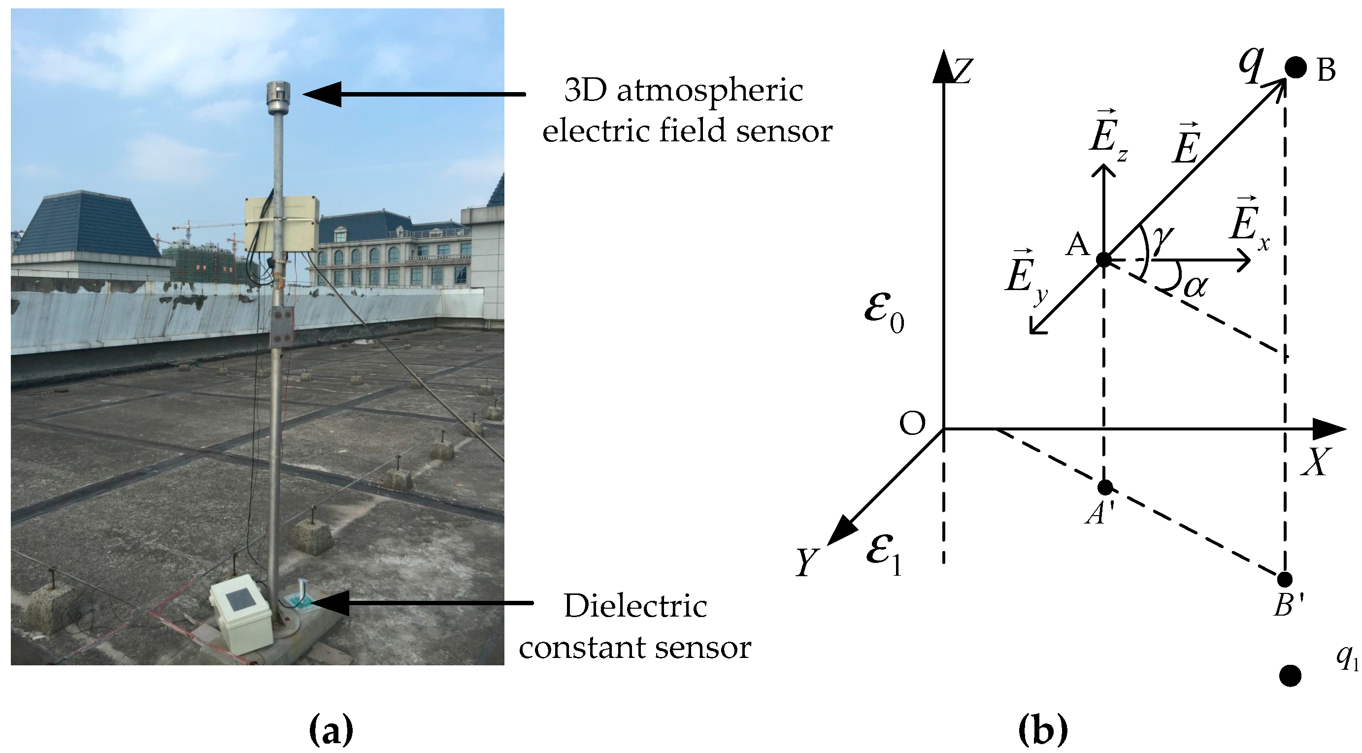
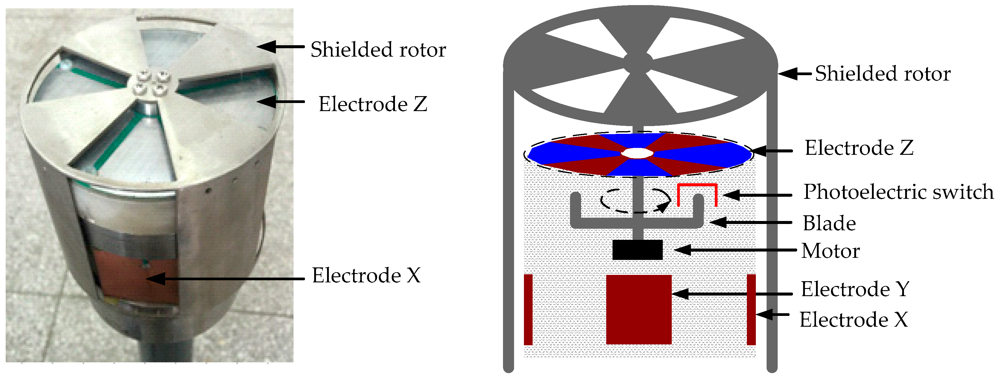
2.1. Principles of Measurement and Calibration
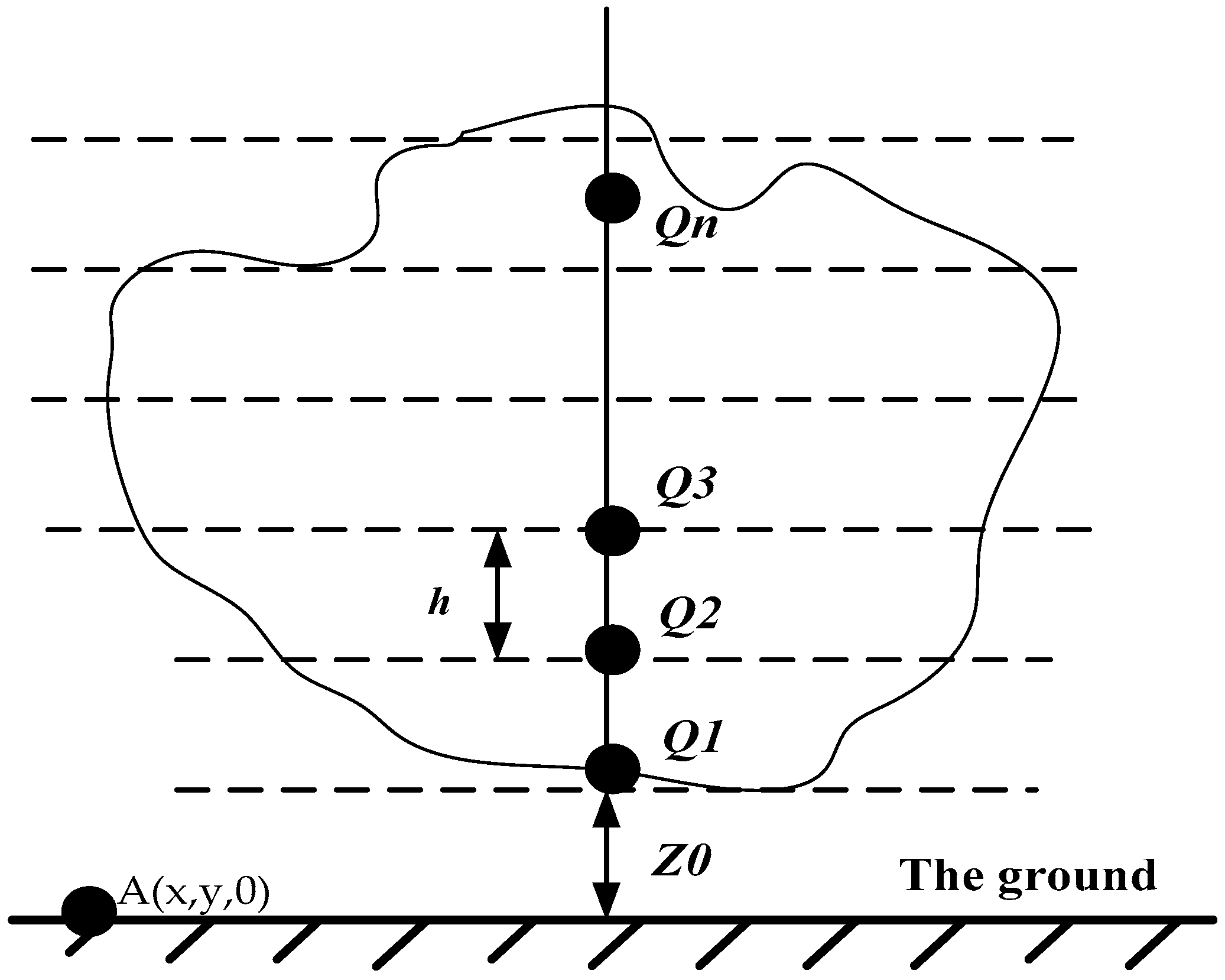
2.2. The Relationship between a Three-Dimensional Atmospheric Electric Field and Thunderstorm Cloud Charge
2.3. Nonlinear Inversion Method for Thunderstorm Cloud Charge Parameters
- (1)
- Initialization of the charge structure parametersIn order to avoid blind searching of structural parameters in the inversion process, the velocity and position of structural parameters need to be initialized. Combined with the classical charged structural parameters of thunderstorm clouds, the inversion parameters are limited to a certain range and , the initial velocity of charge parameter should be [−5, 5], the relative distance between the thunderstorm clouds and three-dimensional atmospheric electric field meter should be assumed. The initial speed of the parameter (, , ) is [−100, 100]. The initial location of the charge parameter is [−30, 30], and the initial location of the relative distance is [−10,000, 10,000].
- (2)
- Fitness function of the three-dimensional electric fieldThe difference between the measured value of the ground electric field and the inverted ground electric field value is defined as a fitness function. When value Y of the fitness function approaches zero, the optimal solution of the parameters can be obtained:
- (3)
- Find the initial extremum of the inversion parameter setAssuming the population size i of the charged structure parameter is 5 and the dimension of search space D is the number of inversion variables, and assuming the thunderstorm cloud is a classical three-layer charged structure, then . That is, the inversion parameter set is {}. If it is a two-layer charged structure, then , that is, the set of inversion parameters is {}.The initial extremum of each parameter of the charged structure is the position of the individual when the initial fitness is optimal, and the global initial extremum Gbest is the position with the best fitness searched in the parameter sets. Let the initial velocity of the structural parameters be , the individual initial extremum is , and the population initial global extremum is .
- (4)
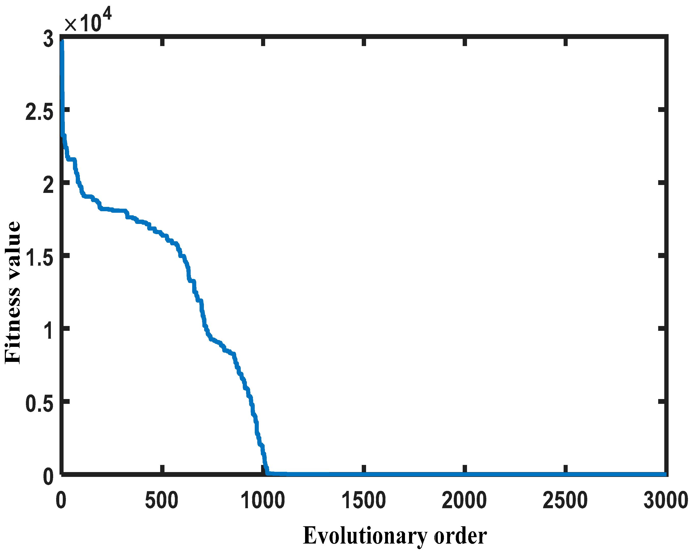
- Update of inversion parametersThe velocity and position of the structural parameters in the iteration are obtained by updating the individual extremum and the global extremum of the iteration. Each time the position is updated, the fitness value is calculated once, and the position update and speed update are shown in Equations (24) and (25):where and are the convergence speeds of the and structural parameters, respectively, and and are the structural parameter values of the and times, respectively. and are acceleration factors that determine the ability of particles to search for global optimal values and individual optimal values. is the number of inverse evolutions, is the weight coefficient, and is the particle at the kth iteration. is the global extremum of the structural parameter set at the iteration.
3. Experimental Results and Analysis
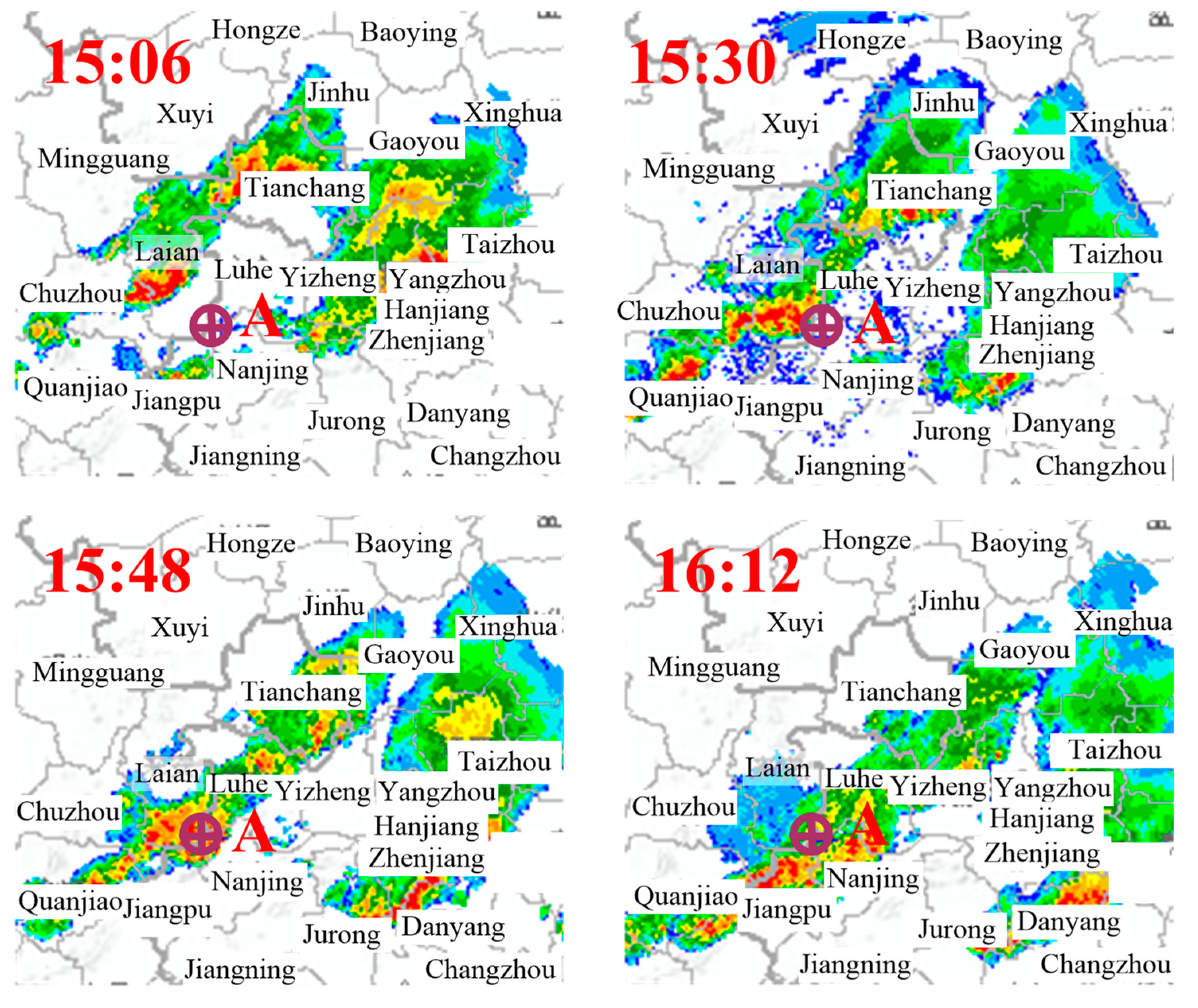
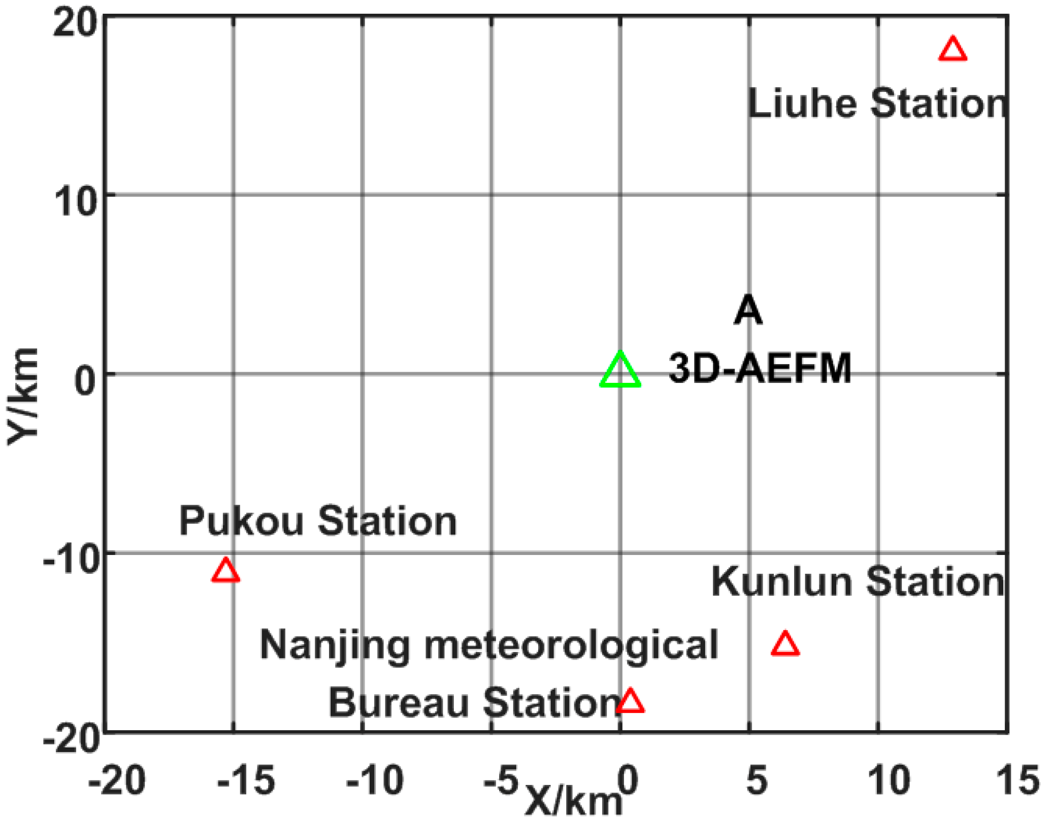
3.1. Three-Dimensional Atmospheric Electric Field and Radar Observation Experiments
3.2. Inversion of the Charge Model
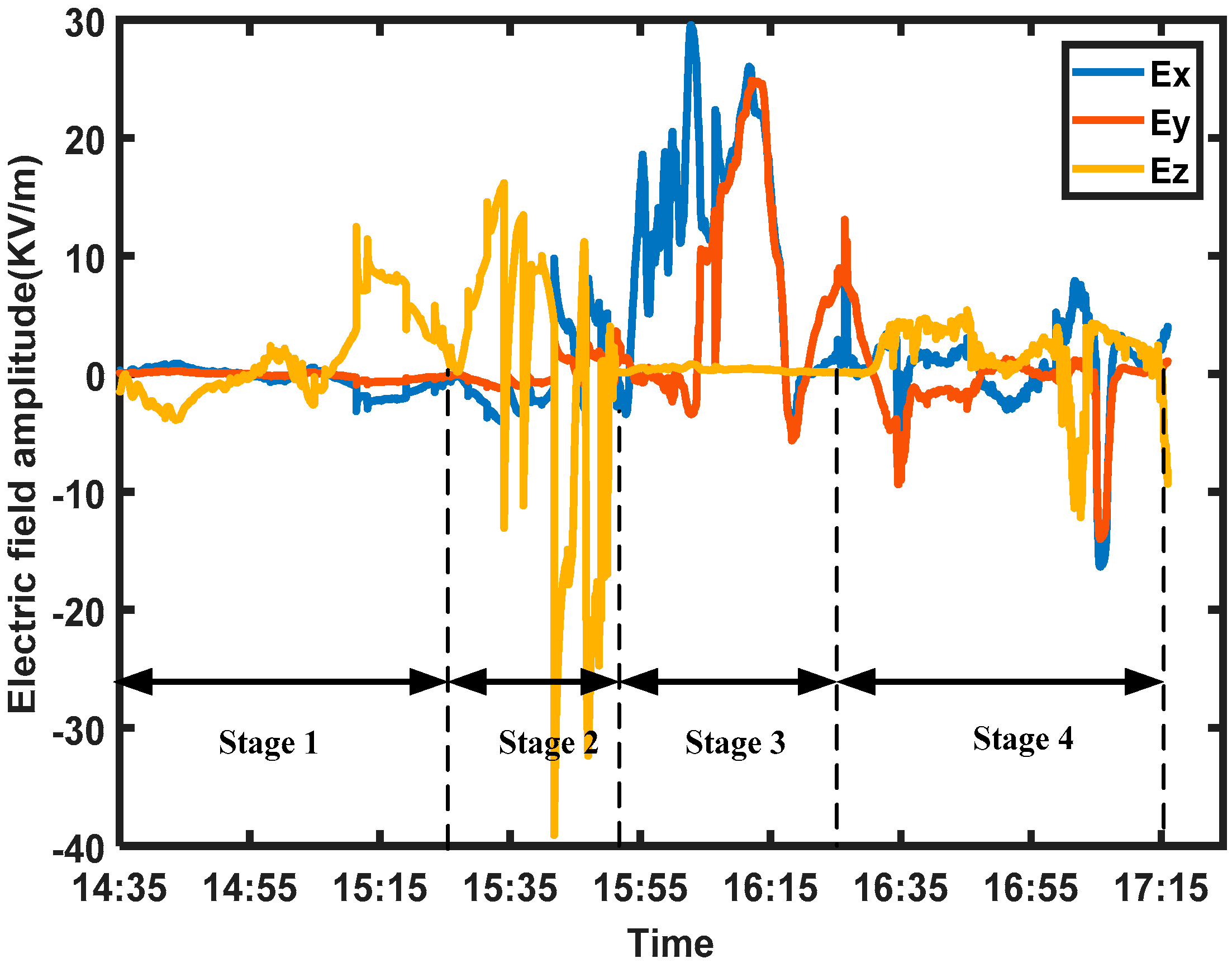
3.3. Comparative Analysis of Electric Field Data
4. Discussion and Conclusions
Author Contributions
Funding
Conflicts of Interest
References
- Simpson, G.; Scrase, F.J. The Distribution of Electricity in Thunderclouds. Proc. R. Soc. Lond. 1937, 161, 309–352. [Google Scholar] [CrossRef]
- Zhao, P.; Yin, Y.; Xiao, H.; Zhou, Y.; Liu, J. Role of Water Vapor Content in the Effects of Aerosol on the Electrification of Thunderstorms: A Numerical Study. Atmosphere 2016, 7, 137. [Google Scholar] [CrossRef]
- Tsenova, B.D.; Barakova, D.; Mitzeva, R. Numerical study on the effect of charge separation at low cloud temperature and effective water content on thunderstorm electrification. Atmos. Res. 2017, 184, 1–14. [Google Scholar] [CrossRef]
- Fan, X.; Zhang, Y.; Zhang, G.; Zheng, D. Lightning Characteristics and Electric Charge Structure of a Hail-Producing Thunderstorm on the Eastern Qinghai–Tibetan Plateau. Atmosphere 2018, 9, 295. [Google Scholar] [CrossRef]
- Gao, W.; Kou, Z.; Ding, P. A Numerical Study of Hail Process Effects on Charge Structure and Lightning Flash Rate of Thunderstorms. In Proceedings of the IEEE Asia-Pacific International Symposium on Electromagnetic Compatibility, Shenzhen, China, 17–21 May 2016; pp. 594–596. [Google Scholar]
- Galanaki, E.; Lagouvardos, K.; Kotroni, V.; Flaounas, E.; Argiriou, A. Thunderstorm climatology in the Mediterranean using cloud-to-ground lightning observations. Atmos. Res. 2018, 207, 136–144. [Google Scholar] [CrossRef]
- Montanya, J.; Bergas, J.; Hermoso, B. Electric field measurements at ground level as a basis for lightning hazard warning. J. Electrostat. 2004, 60, 241–246. [Google Scholar] [CrossRef]
- Ferro, M.A.D.S.; Yamasaki, J.; Pimentel, D.R.M.; Naccarato, K.P.; Saba, M.M.F. Lightning risk warnings based on atmospheric electric field measurements in Brazil. J. Aerosp. Technol. Manag. 2011, 3, 301–310. [Google Scholar] [CrossRef]
- Zeng, Q.; Wang, Z.; Guo, F.; Feng, M.; Zhou, S.; Wang, H.; Xu, D. The application of lightning forecasting based on surface electrostatic field observations and radar data. J. Electrostat. 2013, 71, 6–13. [Google Scholar] [CrossRef]
- Fort, A.; Mugnaini, M.; Vignoli, V.; Rocchi, S.; Perini, F.; Monari, J.; Schiaffino, M.; Fiocchi, F. Design, modeling, and test of a system for atmospheric electric field measurement. IEEE Trans. Instrum. Meas. 2011, 60, 2778–2785. [Google Scholar] [CrossRef]
- Wilson, C.T.R. On some determinations of the sign and magnitude of electric discharges in lightning flashes. Proc. R. Soc. Lond. A 1916, A92, 555–574. [Google Scholar] [CrossRef]
- Chen, Q.; Wei, G.; Wan, H. Quantum inversion of thunderstorm cloud charge model. J. Geophys. 2010, 53, 2237–2243. [Google Scholar]
- Amoruso, V.; Lattarulo, F. Thundercloud pre-stroke electrostatic modeling. J. Electrostat. 2002, 56, 255–276. [Google Scholar] [CrossRef]
- Schumann, C.; Silva, R.B.G.D.; Schulz, W. Electric fields changes produced by positives cloud-to-ground lightning flashes. J. Atmos. Sol. Terr. Phys. 2013, 92, 37–42. [Google Scholar] [CrossRef]
- Yang, D.; Oldenburg, D.W. Electric field data in inductive source electromagnetic surveys. Geophys. Prospect. 2018, 66, 207–225. [Google Scholar] [CrossRef]
- Jayaratne, E.R.; Saunders, C.P.R. The interaction of ice crystals with hailstones in wet growth and its possible role in thunderstorm electrification. Q. J. R. Meteorol. Soc. 2016, 142, 1809–1815. [Google Scholar] [CrossRef]
- Khan, S.U.; Yang, S.; Wang, L.; Liu, L. A Modified Particle Swarm Optimization Algorithm for Global Optimizations of Inverse Problems. IEEE Trans. Magn. 2016, 52, 1–4. [Google Scholar] [CrossRef]
- Pallero, J.L.; Fernández-Muñiz, M.Z.; Cernea, A.; Álvarez-Machancoses, Ó.; Pedruelo-González, L.M.; Bonvalot, S.; Fernández-Martínez, J.L. Particle Swarm Optimization and Uncertainty assessment in Inverse Problems. Entropy 2018, 20, 96. [Google Scholar] [CrossRef]
- Huang, Y.F.; Tan, T.H.; Chen, B.A.; Liu, S.H.; Chen, Y.F. Performance of Resource Allocation in Device-to-Device Communication Systems Based on Particle Swarm Optimization. In Proceedings of the IEEE International Conference on Systems, Man and Cybernetics, Banff, AB, Canada, 5–8 October 2017; pp. 400–404. [Google Scholar]
- Xing, H.; He, G.; Ji, X. Analysis on Electric Field Based on Three Dimensional Atmospheric Electric Field Apparatus. J. Electr. Eng. Technol. 2018, 13, 1696–1703. [Google Scholar]
- Wang, Z.H.; Zeng, Q.F.; Guo, F.X.; Xu, D.P.; Wang, H. A Study of the Electrostatic Field Networking in Three Isolated Thunderstorms. Appl. Mech. Mater. 2013, 239, 775–784. [Google Scholar] [CrossRef]


| 30C | 30 C | −18.38 C | 30 C | 30 C | −18.379 C | 2.856 km | 863.38 m | 1.3115 km |
| Station | Distance (Km) | Official Data (KV/m) | 3D AEFM (KV/m) |
|---|---|---|---|
| Pukou | 18.91 | −1.6 | −1.583 |
| Nanjing Meteorological Bureau | 18.40 | −1.4 | −1.367 |
| Kunlun | 16.49 | −1.9 | −1.931 |
| Liuhe | 22.14 | −0.8 | −0.830 |
© 2018 by the authors. Licensee MDPI, Basel, Switzerland. This article is an open access article distributed under the terms and conditions of the Creative Commons Attribution (CC BY) license (http://creativecommons.org/licenses/by/4.0/).
Share and Cite
Xu, W.; Zhang, C.; Ji, X.; Xing, H. Inversion of a Thunderstorm Cloud Charging Model Based on a 3D Atmospheric Electric Field. Appl. Sci. 2018, 8, 2642. https://doi.org/10.3390/app8122642
Xu W, Zhang C, Ji X, Xing H. Inversion of a Thunderstorm Cloud Charging Model Based on a 3D Atmospheric Electric Field. Applied Sciences. 2018; 8(12):2642. https://doi.org/10.3390/app8122642
Chicago/Turabian StyleXu, Wei, Cancan Zhang, Xinyuan Ji, and Hongyan Xing. 2018. "Inversion of a Thunderstorm Cloud Charging Model Based on a 3D Atmospheric Electric Field" Applied Sciences 8, no. 12: 2642. https://doi.org/10.3390/app8122642
APA StyleXu, W., Zhang, C., Ji, X., & Xing, H. (2018). Inversion of a Thunderstorm Cloud Charging Model Based on a 3D Atmospheric Electric Field. Applied Sciences, 8(12), 2642. https://doi.org/10.3390/app8122642