Abstract
The main aim of this paper was to find the correct method of calculating equations of heat and mass transfer for the adsorption process and to calculate it numerically in reasonable time and with proper accuracy. An adsorption heat pump with a silica gel adsorbent and water adsorbate is discussed. We developed a mathematical model of temperature and uptake changes in the adsorber/desorber comprising the set of heat and mass balance partial differential equations (PDEs), together with the initial and boundary conditions and solved it by the numerical method of lines (NMOL). Spatial discretization was performed with equally spaced axial nodes and the PDEs were reduced to a set of ordinary differential equations (ODEs). We focused on the comparison of results obtained when the set of heat and mass balance ODEs for an adsorber was solved using: (1) the Runge–Kutta fixed step size fourth-order method (RKfixed), (2) the Runge–Kutta–Fehlberg 4.5th-order method with a variable step size (RK45), and (3) the Gear Backward Differentiation Formulae numerical (Gear BDF) methods. In our experience, all three types of ODE numerical methods (RKfixed, RK45, and Gear BDF) can be applied in simple models to model an adsorber with attention on their limitations. The Gear BDF method usually requires much fewer steps than the RK45 method for almost the same calculating time. RK methods require many more steps to obtain results, and the calculating time depends on accuracy or defined time step. Moreover, one should pay attention to the number of nodes or possible oscillations.
1. Introduction
In the face of the growing need to search for ecologically safe sources of energy, research on increasing the use of available low-temperature heat sources by means of various physical processes has intensified. One of them is the adsorption process used, among others, in sorption heat pumps. During the past two decades, adsorption heat pumps have been exploited in theory and in practice to generate cooling [1] and heating [2,3].
Adsorption heat pump applications in cooling refer to useful cooling [4]; chilled water circuits [5,6]; electric vehicle air conditioners [7]; heat rejection systems, such as dry or wet cooling towers or ground coupled heat exchangers [8]; and solar systems as the driving heat source [9,10]. Heating applications of adsorption heat pumps are found in heating systems, waste heat utilization [3,5], low-temperature heat sources (e.g., ground heat exchangers and geothermal water installations [11]) and driving heat sources (e.g., gas furnace) [12]. Adsorptive storage of CO2 can be an interesting example of another application [13].
Adsorption heat pumps have, aside from environmental benefits, several advantages compared to conventional vapor compression systems, such as: simplicity, no moving parts, low maintenance requirements, and the use of stable, nontoxic reactants as adsorbents and adsorbates. They also have disadvantages: discontinuous operation, high design requirements for maintaining the vacuum, large size, and a relatively low coefficient of performance [4,12]. The performance of an adsorption heat pump is controlled by many parameters, such as adsorbent and adsorbate properties, system design, and operating conditions.
Recently, much research has been done on various types of adsorption heat pumps as an alternative to vapor compression systems [14]. Transient modeling of a two-bed silica gel–water adsorption chiller [15] and an adsorbent bed of a zeolite/water cooling system and its numerical modeling of combined heat and mass transfer [16] are examples of one- or two-bed single-stage heat pump modeling. Second law analysis of adsorption cycles with thermal regeneration [17] cannot be overestimated. In order to improve efficiency, more advanced four-bed [18] or even multibed [19] heat pumps have been studied.
Different numerical methods to solve mathematical equations describing adsorption beds or adsorption heat pumps can be found in the literature. For example, a nonuniform temperature, nonuniform pressure dynamic model of heat and mass transfer in compact adsorbent beds was presented by Marletta et al. [20]. The model was described by a set of second-order partial differential equations (PDEs) and solved. Further steps and methods to obtain a numerical solution together with a discussion on parameters affecting the numerical resolution were carefully presented. Dimensionless equations were discretized using a forward difference scheme for time derivatives and boundary conditions for a spatial first-order derivatives quickest upstream difference scheme and a spatial second-order derivatives central difference scheme. To obtain the solution, the alternating direction implicit method was used.
In Restuccia et al. [21], information of the implicit finite difference method of Crank–Nicholson was used to solve the differential equations of the developed model. In a numerical study of a novel cascading adsorption cycle [22], equations representing the model were solved concurrently using the finite difference method. The next example [23] discussed heat transfer in the adsorbent of a waste heat adsorption cooling system, in which the model calculating domain was first discretized in angle, radial, and axial directions, and the three dimensional equations of the adsorbent were calculated by the alternating direction implicit method. The quadratic upstream differencing scheme was used to approximate the convection terms in the equations. Diffusion terms were replaced by the centered difference analogs.
Issues of stability and stiffness of the numerical method were considered in [24]. Integration of partial differential equations with the numerical method of lines is described widely in the literature by Finlayson [25,26] and Schiesser [27]. For many problems described by nonstiff differential system equations, just about any reasonable method is basically stable, for example, the Runge–Kutta fourth-order method, even called the “workhorse” method in MATLAB®. It is a very robust method and the best function to apply as a “first try” for most problems where computational efficiency is of no concern. For convenience or for low precision, adaptive step size Runge–Kutta dominates [28,29].
In many problems, certain parameters change quickly and others change more slowly. For example, in packed-bed chemical reactors, the concentration varies quickly in time, but the temperature does not change rapidly because of the large heat capacity of the solid. Due to the high values of temperature and uptake gradients in an adsorption column (bed), equations describing the heat and mass balance operation of adsorption heat pumps are often described as “stiff” [25]. For stiff problems, many time steps would need to be taken with a small time step, and the calculations would be very slow. The Gear Backward Differentiation Formulae (BDF) method has been developed to overcome this problem [28,29]. Crucial to the success of a stiff integration scheme is an automatic step size adjustment algorithm [30,31].
In this paper, a single-stage adsorption heat pump with a silica gel adsorbent and water adsorbate was considered. The adsorption heat pump consisted of two adsorber/desorber columns, an evaporator, and a condenser.
The mathematical model, developed to calculate temperature and uptake changes in the adsorber/desorber, was established comprising a set of heat and mass balance PDEs together with the initial and boundary conditions and was solved by the numerical method of lines (NMOL). The spatial discretization was performed with equally spaced axial nodes and the PDEs were reduced to a set of ordinary differential equations (ODEs).
Although models of adsorption heat pumps and an adsorber/desorber have been extensively studied in the literature (examples above), very few studies have analyzed the selection of the numerical method and its influence on the calculated results as well as the error of the method. In addition, most of the studies refer to one numerical method, with only a general description. Therefore, a comparison of three numerical methods and their limitations in calculations of the adsorption model is presented in this paper.
In the present paper, the authors focused on the comparison of results obtained when the set of heat and mass balance ODEs was solved using: (1) the Runge–Kutta fixed step size fourth-order method (RKfixed); (2) the Runge–Kutta–Fehlberg 4.5th-order method (RK45) with a variable step size; and (3) the Gear BDF numerical method. The set of balance equations of the adsorber was solved by the previously mentioned numerical ODE subroutines available in the MATLAB® platform. Obtained simulation results from numerical methods were compared with the results from the experiment in [21].
The rest of the paper is organized as follows. The heat and mass balance model of adsorption heat pump performance is established in Section 2. The numerical method for the PDEs of the model is described in Section 3. Comparison of the three numerical methods for the obtained set of ODEs is presented in Section 4. Section 5 presents the numerical calculation results. For the validation of the numerical model, a comparison with the experimental data of Restuccia et al. [21] was made. The main conclusions are summarized in Section 6.
2. Heat and Mass Balance Equations for Adsorber of Adsorption Heat Pump
The ability of a porous solid medium to adsorb volumes of vapor is called adsorption. That process is caused by a mass separation agent (adsorbent) and determined by the quality of the sorbent. At low temperatures, the porous adsorbent adsorbs vapor (adsorbate), while at high temperatures, it desorbs it. This is the basis of the adsorption heat pump with silica gel operation. Vapour molecules (adsorbate) come into contact with adsorbent and are captured by the surfaces’ pores. The use of a porous solid is relatively simple and provides high adsorptive capacity (domain of equilibria of the process). Small pores in a porous medium give rise to diffusional resistance (domain of kinetics of the process). Usually, adsorption in a porous solid medium is performed in columns packed with sorbent particles or fixed bed adsorbers; however, it is primarily a surface rather than a bulk process [32,33].
An adsorption heat pump with silica gel adsorbent and water adsorbate was considered. A silica gel/water pair was used because it is considered suitable for utilizing low-temperature heat sources less than 100 °C (waste heat, geothermal water) due to silica gel’s high capacity at low temperatures and moderate pressures as well as due to temperature for activation and regeneration of this sorbent [32,33,34]. The Dubinin–Astakhov (D–A) adsorption equilibria of the selected adsorbent/adsorbate pair were sourced from the available literature [35,36,37]. The adsorption heat pump under consideration consists of an evaporator, an adsorber/desorber, and a condenser. The configuration of the single stage adsorption heat pump under consideration is presented in Figure 1.
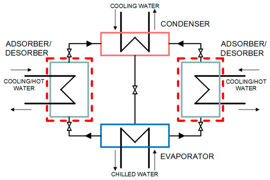
Figure 1.
Configuration of the adsorption heat pump under consideration.
The adsorber/desorber column was encapsulated and contained tubes with deposited adsorbent (silica gel). The design of the adsorber/desorber tube arrangement is presented in Figure 2.
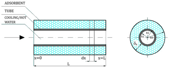
Figure 2.
Design of the adsorber/desorber element (tube with deposited silica gel bed).
The adsorption heat pump’s operation mechanism included a series of cyclic transient processes. These processes ran at different temperatures and pressure levels. The adsorption process was followed by a preheating process to raise the temperature and pressure of the sorption reactor to the condenser pressure. The desorption process began afterwards. Next, the precooling process started, which cooled down the adsorber/desorber so that it would have a low pressure equal to the evaporator pressure. When the refrigerant from the evaporator was transported to the condenser and returned back to the evaporator, one cycle was completed and the circuit was restarted. A one-dimensional numerical model was created to describe the temperature and uptake changes in the adsorber/desorber and consequently to describe the performance of the adsorption heat pump. Only heat and mass transfer were taken into account during operation of the assumed adsorption heat pump.
Noting that although the advanced models of these components are more accurate in simulation, they are too time-consuming in the research process, which may reduce the possibility of finding better solutions in a limited time. Thus, the following main simplifying assumptions were made:
- Pressure losses of vapor at the adsorbate flows both from the evaporator to the silica gel grains and from the grains to the condenser are negligibly small.
- During the adsorption process, pressure inside the adsorber/desorber equals that inside the evaporator. During the desorption process, pressure inside the adsorber/desorber equals that inside the condenser.
- The average temperature of reactor’s cooling and hot water as well as the average specific heat of the adsorbent and water are constant.
- Thermal conductivity of the adsorbent is constant.
- The temperature inside evaporator as well as inside condenser is constant.
- Vapor temperature and pressure during the adsorption process are equal to the evaporator temperature and pressure.
- Vapor temperature during desorption process is related to the heat balance of the bed, and the vapor pressure during desorption process is equal to the condenser pressure.
- Switching between adsorption and desorption cycles (cooling water is switched to hot water) takes place in an instant.
- Desorption kinetics is described and modeled as the adsorption kinetics.
The heat and mass balance PDEs were formulated for calculation element dx (Figure 2). Those equations took into account: heat flow supplied to the process, the heat flow generated, the heat flow discharged from the process, and the heat flow accumulated.
In this article, the authors focused on describing methods for solving the set of partial differential equations and other assumptions. A detailed description of the developed model can be found in articles [38,39], where the performance of two-bed as well as six-bed single-stage adsorption heat pumps were considered. The set of heat and mass balance equations for the adsorber subelement dx (Figure 2) of the considered adsorption heat pump can be described by
where constant parameters , , and from the above set are listed in Table 1. Equation (1) is the fluid (water) energy balance equation, where is the fluid/metal tube heat transfer coefficient, is the fluid thermal conductivity, and is the tube internal radius. Equation (2) is the heat energy balance for the metal tube, where is the adsorbent/fluid heat transfer coefficient, is the metal tube thermal conductivity, and is the tube outer radius. Equation (3) is the heat and mass balance equation for the adsorbent, where is the adsorbent thermal conductivity and is the isosteric heat of adsorption. Equation (4) is an adsorption and desorption process dynamics described by the application of the linear driving force model (LDF), where is the mass transport equation and [16]. This equation calculates the time dependent change in concentration (uptake) for the working bed (silica gel) subelement. The heat of adsorption for both the adsorption and desorption processes was determined by the Clausius–Clapeyron equation [33].

Table 1.
Constant parameters from the set of heat and mass balance partial differential equations of the adsorbent model.
All components were assumed at an initial temperature of , while initial uptake was considered for initial pressure :
For adsorption and desorption pressures, it was assumed
The boundary conditions for the fluid, considering the temperature of the process water supplied to the column, were equal to the driving heat temperature:
The model assumed perfect insulation. Therefore, the heat transfer to and from the ambient was equal to zero:
3. Numerical Method for the PDEs
The NMOL is a well-established technique (or rather a semianalytical method) for solving partial differential equations by typically using a finite difference relationship for the spatial derivatives and ordinary differential equations for the time derivative [27,40]. This is essentially a two-step process: the spatial (boundary value) derivatives are approximated algebraically, for example, by finite difference or a flux limiter, on a spatial grid. The resulting system of ODEs in the initial value variable (typically time) is then integrated by an initial value ODE integrator (e.g., Euler’s method, RK45, Backward Differentiation Formulae method). All of the major classes of PDEs can be accommodated (elliptic, hyperbolic, and parabolic) [27].
The semianalytical character of the formulation leads to a simple and compact algorithm, which yields accurate results with less computational effort than other techniques. In NMOL, by separating discretization of space and time, it is easy to establish stability and convergence for a wide range of problems [27,41].
The mathematical model was established comprising the set of heat and mass balance PDEs (Equations (1)–(4)), together with the initial and boundary conditions (Equations (5)–(12)). The model was solved by the NMOL. The first step was discretization of the x-variable (Figure 3).
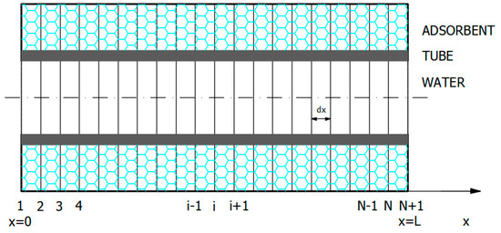
Figure 3.
Illustration of adsorber discretization in the x-direction (numerical method of lines, NMOL).
The region was divided into strips by N sections with N + 1 nodes, where was the spacing between the discretized line:
To avoid meaningless results (characteristic in adsorption equation oscillation) or numerical diffusion, especially with respect to convection segments [27], in this work, first- and second-order derivatives (1–4) used the five-point difference scheme of four-order truncation error discretization.
Let be any of the functions , and means here . Replacing the first- and second-order derivatives at nodes i = 3 to N − 1 with respect to using a central five-point difference formula becomes [27]
Replacing the first- and second-order derivatives at nodes i = 1 and i = 2 using a forward five-point difference formula becomes, respectively,
The first- and second-order derivatives at nodes N and N + 1, using a backward five-point difference formula, can be rewritten, respectively, as follows:
Equations (14)–(23) are characterized by a four-order truncation error of approximation. The boundary conditions represented by Equations (10)–(12) at nodes I = 1 and N + 1 can be generally written for function , respectively, as follows:
hence:
hence:
The functions (from Equations (1)–(4)) were stored as an array of indexes , where refers to the time and to the spatial node. To summarize, the spatial discretization was performed with equally spaced axial nodes and the PDEs were reduced to a set of ODEs.
4. Numerical Method for the ODEs
There are many mathematical types of software that have built-in functions to perform numerical integration of ODEs. The obtained set of ODEs was solved numerically in the MATLAB R2018b (MathWorks®, Massachusetts, USA) platform using two different in problem nature solvers: the Runge–Kutta fourth-order algorithm (RKfixed classical fixed step size and RK45 adaptive step size) and the Gear BDF algorithm.
4.1. Runge–Kutta Fourth-Order Method (Classical)
Runge–Kutta methods propagate a solution over an interval by combining the information from several Euler-style steps and then using the information obtained to match a Taylor series expansion up to some higher order. The common opinion of Runge–Kutta is that it is the best function to apply as a first try for most problems or for trivial problems where computational efficiency is of no concern and succeeds virtually very often. However, it is not usually the fastest method, except when moderate accuracy 1e-5is required [30].
The classical Runge–Kutta method is based on the Simpson quadrature rule and uses four explicit stages, hence four function evaluations per step, to achieve accuracy. Local truncation error is fourth order if has five continuous derivatives. In general, the classical fourth-order Runge–Kutta method requires four evaluations K of the right-hand side of the differential equation per time step [25,26,27].
The Runge–Kutta classical fixed time step size method for the discussed set of ODE balance equations was written as
where is the increase of the independent variable , and are time derivatives of searched functions implicitly dependent on time and where n is the time point of the known values of the function and n + 1 is the next time point. The resulting equations were implemented manually as a code and solved in MATLAB® platform.
4.2. Runge–Kutta–Fehlberg 4.5th-Order Method
A popular method for integrating equations in time is the Runge–Kutta–Fehlberg (RK45 order) method. This is a fourth-order method but achieves fifth-order accuracy. Adaptive step size methods allow changing the step size during the integration. The time step is changed to guarantee the accuracy of the calculation. The accuracy is estimated at each step, and the step size is reduced to meet the specified accuracy. The method has a stability limitation. The variable step size overcomes two of the problems—knowing what step size to use and using a small enough step size to guarantee a specified accuracy [25,26,27].
The general form of a Runge–Kutta–Fehlberg 4.5th-order method with adaptive step size is widely described in the literature, for example, in the extra materials described by Finlayson in [25]. For the results, a MATLAB® subroutine called “ode45” was implemented.
4.3. Gear Method (Backward Differentiation Formulae)
The BDF implicit method is one of many linear multistep methods (LMM). It is called BDF because it differentiates the solution using past (backward) values. The simplest BDF method (BDF1) is Backward Euler (BE), but the Gear method is well known and has been validated especially for stiff differential equations systems. The disadvantage of that method is the fact that it requires at each time step the solution of a nonlinear system of equations [28,29,42].
The general form of the Gear fourth-order method with variable step size is described in the literature, for example, in the extra materials in [25,28]. Methods like this are also implemented in MATLAB® (i.e., “ode15s”, a subroutine that adjusts the step size to maintain a specified accuracy).
The set of equations mentioned earlier was implemented and solved by the fourth-order Gear BDF method in the “ode15s” subroutine of the MATLAB® platform.
5. Results
The fixed as well as the adaptive step size fourth-order methods were successfully implemented and tested on the experimental results [43]. For validation of the numerical model, a comparison with the experimental data of Restuccia et al. [21] was made. There, the experimental setup consisted of a lab-scale single-bed module using a pack of finned stainless-steel tubes and the composite sorbent SWS-1L. The geometrical specifications and the operating conditions of the numerical model were adjusted to their counterparts in the tested lab-scale chilling module with the adsorption/desorption bed. Inlet water heating and cooling temperatures were adjusted to 95 and 40 °C. Other settings, such as time control for isobaric and isosteric phases, that were the same as those in Restuccia et al. [21] were also considered.
The comparison between the time variations of the presented numerical methods and the experimental averaged bed temperatures is shown in Figure 4. To achieve results, the implemented Runge–Kutta fourth-order method, with the fixed time step , required 132,952 steps; RK45, with (1e-5) accuracy, required 206,423 steps; and the Gear BDF method (accuracy 1e-2) required only 132 steps (for N = 20). The accuracy was adapted to the method to make it possible to obtain results, which is associated with stability, stiffness, and other characteristic limitations of each of the presented numerical methods’ calculating results based on the one-dimensional model of adsorber described above. Runge–Kutta fourth-order methods (fixed time step as well adaptive step) obtained results that were very similar, while the results based on the Gear BDF method were slightly different in several points from the Runge–Kutta results but even closer to experimental points.
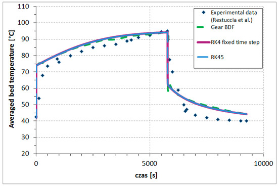
Figure 4.
Comparison between the time variations of the presented numerical methods and experimental averaged bed temperatures. (Restuccia et al. [21]).
The reasons for the differences between the results of the experiment and the results of the numerical methods of the described model can be divided into three categories.
First, the differences were related to the simplifying assumptions adopted in the model (described in point 2) regarding the constancy of some parameters, such as density, thermal conductivity, or specific heat, at variable temperatures and pressures. A simplified description of the adsorption and desorption pressures and temperatures was also assumed. The assumption of rapidly switching between adsorption and desorption cycles (cooling water is switched to hot water) also had an impact. Another aspect was the assumption of the desorption kinetics modeled as the adsorption kinetics (Equation (4)), which was a significant simplification. Second, the experimental data for validation of the model was reconstructed based on the literature and on the description of the test stand and measurement results given by the authors of [21]. According to Restuccia et al. [21], the typical experimental error in the various tests was about 5%. Third, the discretization methods were characterized by fourth-order truncation error of approximation.
In conclusion, in order to reduce the difference, a model describing the more complex heat and mass transfer could be prepared. However, the presented difference between the results of the experiment and the numerical model was at an acceptable level. Reasonable agreement between the results is an indication of proper mathematical modeling and the accuracy of the numerical schemes.
For the considered one-dimensional model of the adsorber in the adsorption heat pump, one calculation case of driving parameters was chosen to investigate limitations in use of the presented numerical methods.
The variables studied were: temperature of desorption, which was equal to the hot driving water temperature ; temperature of the adsorption process, equal to the cooling water temperature ; temperature of evaporation ; and temperature of condensation . Cycle duration in the examined case was as well as heating/cooling medium (water) flow rate . Parameters of adsorption equilibrium described by the Dubinin–Astakhov (D–A) equation used for the calculations were: limiting adsorption amount , characteristic energy of the adsorbent , constant in the D–A Equation , process constant , and activation energy [15,34]. Other parameter values used for the calculations are given in Table 2. Due to the initial starter cycles and the characteristics of the adsorption devices, the calculations were carried out for 10 adsorber/desorber cycles. To compare the results of the numerical methods in the last two cycles, stable operation of the modeled adsorption column (adsorber/desorber) was used.
Table 2.
Parameters used in the calculation (sourced from [15,34,44,45]).
Figure 5 shows the results comparison of the calculated temperatures of the modeled fluid (water) , metal tube , and adsorbent in function of time based on the ODE numerical methods RKfixed, RK45, and Gear BDF for the described one-dimensional model of the adsorber. Temperatures at the beginning of the adsorption column are presented in Figure 5a, while temperatures in the middle and at the end of the adsorption column are presented in Figure 5b,c, respectively. The graphs in Figure 5 show the temperatures curves in the following order (as viewed in desorption—the upper part of the graph): the highest curves are fluid temperatures, the middle curves shows the metal tube temperatures, and the bottom curves show the adsorbent temperatures. It can be observed that when the change of for x = 0, i = 1 takes place, the oscillations of , , and appear. Such oscillations are characteristic of numerical solutions of so-called stiff problems. Stiffness is a property of a system of differential equations rather than its solution. For such problems, an implicit multistep method (e.g., Gear BDF) rather than explicit multistep methods (e.g., RKfixed or RK45) should be used.
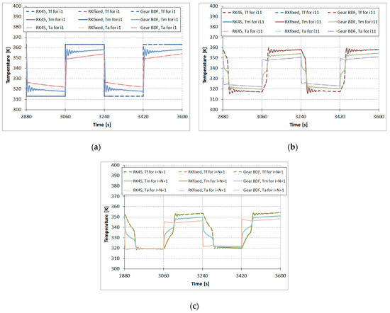
Figure 5.
Results comparison of the Runge–Kutta fixed step size fourth-order (RKfixed), the Runge–Kutta–Fehlberg 4.5th-order method with a variable step size (RK45), and the Gear Backward Differentiation Formulae (Gear BDF) methods, calculated temperatures of the modeled fluid (water) , metal tube , and adsorbent , N = 20: (a) node i = 1, (b) node i = 11, and (c) node i = 21.
Figure 6 shows calculated uptake for the nodes i = 1 (lowest curve), i = 11 (in the middle), and i = 21 (highest curve) of the adsorber column.
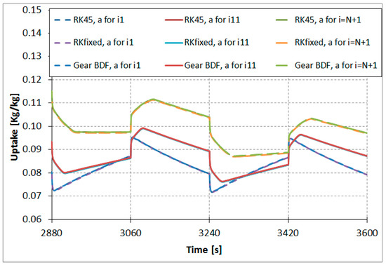
Figure 6.
Results comparison of RKfixed, RK45, and Gear BDF methods, calculated uptake in nodes i = 1, i = 11, and i = 21 (N = 20).
For the above-introduced calculation case of the adsorption heat pump, there was no significant difference in results based on the discussed fixed RK method as well as adaptive step size numerical fourth-order methods. The absolute temperature difference was smaller than 1% and was irrelevant from the perspective of engineering applications. In our experience, the Runge–Kutta and Gear routines give adequate results for relatively simple one-dimensional adsorption models.
Table 3 presents additional comparisons of discretization, accuracy, CPU (Central Processing Unit) process time, and number of steps for the RKfixed, RK45, Gear BDF numerical methods as well as some of limitations. The Gear BDF routine “ode15s” (BDF “on”) integrated a set of equations in the smallest number of steps and had the shortest processing time. For example, for the 20 sections in MOL (N = 20) and accuracy (1e-7), it takes 9525 steps in 10 s of CPU time. By contrast, the RK45 routine “ode45” requires 16,776 steps, while RKfixed time step size (dt = 0.1 s) takes 36,010 steps in 122 s of CPU time.
Table 3.
Comparison of discretization, accuracy, process time, and numbers of steps for the following numerical methods: RKfixed, RK45, and Gear BDF (Processor Intel, Xeon (R) X5690, 3.46 GHz, 8 GB RAM, 64-bits System).
Additionally, the research identified restrictions on the use of all these numerical methods. Examples of limitations are presented in Table 3. In the Runge–Kutta fourth-order fixed time step method, for the above-introduced calculation case of adsorption, it was not possible to obtain results for discretization N < 5, fixed time step > 1 s or accuracy ≤ (1e-4). In the range of 5 ≤ N ≤ 10, there was no realistic result. In the Runge–Kutta–Fehlberg 4.5th-order adaptive step method, there were no results for N < 18 or . Since this method is mainly used for nonstiff systems of equations—and apparently for listed parameters, the stiffness of solving systems of equations is growing—there is a decreasing possibility of obtaining real results with this method.
For use in a wider operating range, there is the Gear BDF method. With that method, results could be obtained for the accuracy range from (1e-1) to (1e-8) or even higher, and for discretization, from N ≥ 5 to N ≥ 40, but the advantage is to take into account reasonable processing time.
The results comparison of the RKfixed, RK45, and Gear BDF methods in different accuracies and discretizations for the calculated averaged temperatures of the modeled fluid (water) (Figure 7), calculated averaged adsorption bed temperatures (Figure 8), as well as averaged water vapor uptake on the silica gel adsorbent (Figure 9) shows small differences in the course of the curves, particularly in the area of undesired oscillations. There was one main exception; the results obtained from RKfixed (N20, time step 1 s) differed from the other results by about 10 K for adsorbent temperature and about 9% absolute difference for the uptake. This means that the time step 1 s is overly large and the results are overly rough.
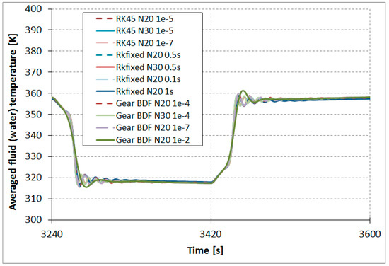
Figure 7.
Results comparison of the RKfixed, RK45, and Gear BDF methods in different accuracies and discretizations, calculated averaged temperatures of the modeled fluid (water) .
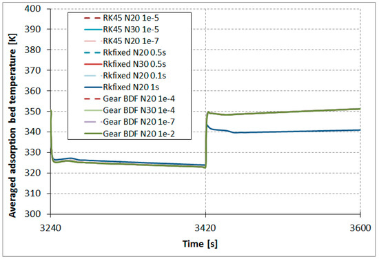
Figure 8.
Results comparison of the RKfixed, RK45, and Gear BDF methods in different accuracies and discretizations, calculated averaged adsorption bed temperatures .
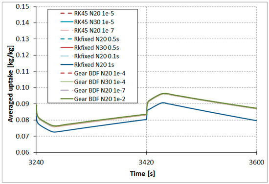
Figure 9.
Results comparison of the RKfixed, RK45, and Gear BDF methods in different accuracies and discretizations, calculated averaged uptake .
6. Conclusions
The main aim of this work was to find the correct method of calculating equations of heat and mass transfer for the adsorption process and to calculate it numerically in a reasonable amount of time and with proper accuracy. The calculation of the coefficient of performance is a secondary effect to the one presented in the article, but it is widely described in previous papers [38,39], where the performance of two-bed as well six-bed single-stage adsorption heat pumps was considered in detail. The obtained results allowed us to calculate the COP for the abovementioned case of parameters. Based on the RKfixed method, for cooling applications, the results was ; so, for heating applications, . The set of balance equations of the adsorber was solved by the previously mentioned numerical ODE subroutines available in the MATLAB® platform. For the Runge–Kutta fixed step size fourth-order method, the resulting equations were implemented as code and solved in MATLAB®. For the Runge–Kutta method with a variable step size (Runge–Kutta–Fehlberg 4.5th-order method), the MATLAB® subroutine called “ode45” was implemented. The fourth-order Gear BDF method was implemented in the “ode15s“ (BDF “on“) subroutine of MATLAB®. The fixed as well as the adaptive time step fourth-order methods were implemented and compared successfully with the experimental data.
It can be observed that, when the change of water temperature for adsorption (or for desorption) starts, oscillations of adsorbent, tube, and vapor temperatures appear. Such oscillations are characteristic for numerical solutions of so-called stiff problems. Stiffness is a property of a system of differential equations rather than its solution. For such problems, an implicit multistep method (e.g., Gear BDF) rather than explicit multistep methods (e.g., RKfixed or RK45) should be used.
It is possible to use Runge–Kutta methods to solve systems of equations for an adsorber in adsorption heat pumps, which are characterized by growing stiffness with different parameters. However, taking into account the limited scope of these methods, this decreases the possibility of obtaining real results in an acceptable processing time. For use in a wider operating range and in reasonable operating time (less time steps), the Gear BDF method is better. For example, the Gear BDF routine integrated the presented set of equations in only 3633 steps (N = 20, 1e-4). By contrast, the Runge–Kutta–Fehlberg 4.5th routine required 9537 steps, while Runge–Kutta fixed time step size (dt = 0.5 s) took 7201 steps. The error of the methods depends on the step size. A small step size leads to better precision, but requires greater CPU time.
For use in a wider operating range, the Gear BDF method is preferred. With that method, results could be obtained for the accuracy range from (1e-1) to (1e-8) or even higher, and for discretization, from N ≥ 5 to N ≥ 40. However, the advantage is to take into account reasonable processing time.
The results comparison of the RKfixed, RK45, and Gear BDF methods in different accuracies and discretizations for calculated averaged temperatures of the modeled fluid (water) (Figure 7), calculated averaged adsorption bed temperatures (Figure 8), as well as averaged water vapor uptake on silica gel adsorbent (Figure 9) shows small differences in the course of the curves, particularly in the area of undesired oscillations. There is one main exception; the results obtained from the RKfixed (N20, time step 1 s) differ from the other results by about 10 K for adsorbent temperature and about 9% absolute difference for the uptake. This means that the time step 1 s is overly large and the results are overly rough.
In our experience, the Runge–Kutta and Gear routines give adequate results for relatively simple one-dimensional models of an adsorber in an adsorption heat pump. In general, all three types of ODE numerical methods (RKfixed, RK45, and Gear BDF) can be applied in simple models (one-dimensional) to model an adsorption column in an adsorption heat pump, with attention on their limitations. The Gear BDF method usually requires much fewer steps than the RK45 method for almost the same CPU time, and the results are without oscillations for low accuracy. RK methods require many more steps to obtain results, but the CPU time depends on the accuracy or defined time step. Moreover, one should pay attention to the number of nodes or possible oscillations.
For the introduced above calculation case of the adsorption heat pump, there is no significant difference in results based on the discussed fixed as well as adaptive step size numerical fourth-order methods. The absolute temperature difference is smaller than 1%, and is irrelevant from the perspective of engineering applications. In our experience, the Runge–Kutta and Gear routines give adequate results for relatively simple one-dimensional adsorption model.
Since the appropriate numerical method has been developed for modeling the adsorption process, future research should focus on developing multibed adsorption systems. It could be advantageous in respect to its power output control and its efficiency optimization.
Author Contributions
K.Z.-M. provides conceptualization, resources, data curation, methodology, validation, formal analysis and calculations, writing—original draft preparation and review editing, visualization. D.M.-M. provides methodology, formal analysis and calculations, software, writing—review and editing.
Funding
This research received no external funding.
Conflicts of Interest
The authors declare no conflict of interest.
Nomenclature
| mass/amount adsorbed/desorbed on adsorbent at time τ, (uptake) | |
| limiting adsorption amount, | |
| characteristic energy of the adsorbent, | |
| specific heat, | |
| process constant, | |
| calculation element (spatial), m | |
| calculation element (time), s | |
| activation energy, | |
| function, - | |
| isosteric heat of adsorption, | |
| i | node, |
| length, | |
| mass flow rate, | |
| sections, | |
| constant in the D–A equation, | |
| truncation error of approximation | |
| pressure, | |
| heat, | |
| gas constant, | |
| R1 | tube internal radius, |
| R2 | tube outer radius, |
| R3 | adsorber outer radius, |
| particle radius, | |
| temperature, | |
| Greek letters | |
| heat transfer coefficient, | |
| thermal conductivity, | |
| ρ | density, |
| time, | |
| Subscripts | |
| a | adsorbent |
| ads | adsorption |
| cond | condenser |
| des | desorption |
| eq | equilibrium |
| evap | evaporator |
| f | fluid (water) |
| m | metal tube/pipe |
Abbreviations
| BDF | Backward Differentiation Formulae |
| BE | Backward Euler Method |
| CPU | Central Processing Unit |
| D–A | Dubinin–Astakhov |
| LMM | Linear Multistep Method |
| NMOL | Numerical Method of Lines |
| ODEs | Ordinary Differential Equations |
| PDEs | Partial Differential Equations |
| RKfixed | Runge–Kutta fixed step size fourth-order Method |
| RK45 | Runge–Kutta–Fehlberg 4.5th-order Method |
References
- Restuccia, G.; Cacciola, G. Performances of adsorption systems for ambient heating and air conditioning. Int. J. Refrig. 1999, 22, 18–26. [Google Scholar] [CrossRef]
- Pons, M.; Meunier, F.; Cacciola, G.; Critoph, R.E.; Groll, M.; Puigjaner, L.; Spinner, B.; Ziegler, F. Thermodynamic based comparison of sorption systems for cooling and heat pumping. Int. J. Refrig. 1999, 22, 5–17. [Google Scholar] [CrossRef]
- Zwarycz-Makles, K.; Kuczynski, K.; Ambrozek, B. Modeling of adsorption heat pump integrated with district heating network. In Proceedings of the 26th International Conference on Efficiency, Cost, Optimization, Simulation and Environmental Impact of Energy Systems (ECOS 2013), Guilin, China, 16–19 July 2013. [Google Scholar]
- Wongsuwan, W.; Kumar, S.; Neveu, P.; Meunier, F. A review of chemical heat pump technology and applications. Appl. Therm. Eng. 2001, 21, 1489–1519. [Google Scholar] [CrossRef]
- Nunez, T.; Mittelbach, W.; Henning, H.M. Development of an adsorption chiller and heat pump for domestic heating adn air-conditioning applications. Appl. Therm. Eng. 2007, 27, 2205–2212. [Google Scholar] [CrossRef]
- Wang, D.; Zhang, J.; Xia, Y.; Han, Y.; Wang, S. Investigation of adsorption performance deterioration in silica gel–water adsorption refrigeration. Energy Convers. Manag. 2012, 58, 157–162. [Google Scholar] [CrossRef]
- Aceves, S.M. An Analytical Comparison of Adsorption and Vapor Compression Air Conditioners for Electric Vehicle Applications. J. Energy Resour. Technol. 1996, 118, 16–21. [Google Scholar] [CrossRef]
- Rege, S.U.; Yang, R.T.; Buzanowski, M.A. Sorbents for air prepurification in air separation. Chem. Eng. Sci. 2000, 55, 4827–4838. [Google Scholar] [CrossRef]
- Sekret, R.; Turski, M. Research on an adsorption cooling system supplied by solar energy. Energy Build. 2012, 51, 15–20. [Google Scholar] [CrossRef]
- Sarbu, I.; Sebarchievici, C. Review of solar refrigeration and cooling systems. Energy Build. 2013, 67, 286–297. [Google Scholar] [CrossRef]
- Zwarycz-Makles, K.; Szaflik, W. Comparison of Analytical and Numerical Models of Adsorber/desorber of Silica Gel-water Adsorption Heat Pump. J. Sustain. Dev. Energy Water Environ. Syst. 2017, 5, 69–88. [Google Scholar] [CrossRef]
- Demir, H.; Mobedi, M.; Ulku, S. A review on adsorption heat pump: Problems and solutions. Renew. Sustain. Energy Rev. 2008, 12, 2381–2403. [Google Scholar] [CrossRef]
- Ben-Mansour, R.; Olufemi Eyitope, B.; Antar, M.A. Simulation of Adsorptive Storage of CO2 in Fixed Bed of MOF-5. J. Energy Resour. Technol. 2015, 138, 012001. [Google Scholar] [CrossRef]
- Chahbani, M.H.; Labidi, J.; Paris, J. Modeling of adsorption heat pumps with heat regeneration. Appl. Therm. Eng. 2004, 24, 431–447. [Google Scholar] [CrossRef]
- Chua, H.T.; Ng, K.C.; Wang, W.; Yap, C.; Wang, X.L. Transient modeling of a two-bed silica gel–water adsorption chiller. Int. J. Heat Mass Transf. 2004, 47, 659–669. [Google Scholar] [CrossRef]
- Leong, K.C.; Liu, Y. Numerical modeling of combined heat and mass transfer in the adsorbent bed of a zeolite/water cooling system. Appl. Therm. Eng. 2004, 24, 2359–2374. [Google Scholar] [CrossRef]
- Pons, M. Second Law Analysis of Adsorption Cycles with Thermal Regeneration. J. Energy Resour. Technol. 1996, 118, 229–236. [Google Scholar] [CrossRef]
- Ng, K.C.; Wang, X.; Lim, Y.S.; Saha, B.B.; Chakarborty, A.; Koyama, S.; Akisawa, A.; Kashiwagi, T. Experimental study on performance improvement of a four-bed adsorption chiller by using heat and mass recovery. Int. J. Heat Mass Transf. 2006, 49, 3343–3348. [Google Scholar] [CrossRef]
- Akisawa, A.; Miyazaki, T. Mutli-bed adsorption heat pump cycles and their optimal operation. In Advances in Adsorption Technology; Saha, B.B., Ng, K.C., Eds.; Nova Science Publishers Inc.: Hauppauge, NY, USA, 2010; pp. 241–279. ISBN 978-1-60876-833-2. [Google Scholar]
- Marletta, L.; Maggio, G.; Freni, A.; Ingrasciotta, M.; Restuccia, G. A non-uniform temperature non-uniform pressure dynamic model of heat and mass transfer in compact adsorbent beds. Int. J. Heat Mass Transf. 2002, 45, 3321–3330. [Google Scholar] [CrossRef]
- Restuccia, G.; Freni, A.; Vasta, S.; Aristov, Y. Selective water sorbent for solid sorption chiller: Experimental results and modelling. Int. J. Refrig. 2004, 27, 284–293. [Google Scholar] [CrossRef]
- Liu, Y.; Leong, K.C. Numerical study of a novel cascading adsorption cycle. Int. J. Refrig. 2006, 29, 250–259. [Google Scholar] [CrossRef]
- Zhang, L.Z.; Wang, L. Momentum and heat transfer in the adsorbent of a waste-heat adsorption cooling system. Energy 1999, 24, 605–624. [Google Scholar] [CrossRef]
- Eberly, D. Stability Analysis for Systems of Differential Equations. Geometric Tools, LLC., 2006. Available online: http://www.geometrictools.com/ (accessed on 23 July 2018).
- Finlayson, B.A. Nonlinear Analysis in Chemical Engineering; McGraw-Hill: New York, NY, USA, 1980; ISBN 978-0070209152. [Google Scholar]
- Finlayson, B.A. Introduction to Chemical Engineering Computing; John Wiley & Sons, Inc.: Hoboken, NJ, USA, 2006; ISBN 978-0-471-74062-9. [Google Scholar]
- Schiesser, W.E. Numerical Method of Lines Integration of Partial Differential Equations; Academic Press: San Diego, CA, USA, 1991; Available online: http://www.lehigh.edu/~wes1/apci/28apr00.pdf (accessed on 23 July 2018).
- Gear, C.W. Numerical Initial Value Problems in Ordinary Differential Equations; Prentice Hall: Englewood Cliffs, NJ, USA, 1971; ISBN 013-626606-1. [Google Scholar]
- Forsythe, G.; Malcolm, M.; Moler, C. Computer Methods for Mathematical Computation; Prentice-Hall: Englewood Cliffs, NJ, USA, 1977; ISBN 0131653326. [Google Scholar]
- Press, W.H.; Teukolsky, S.A.; Vetterling, W.T.; Flannery, B.P. Numerical Recipes in Fortran 77: The Art of Scientific Computing, 2nd ed.; Fortran Numerical Recipes; Cambridge University Press: Cambridge, UK, 1992; Volume 1, ISBN 0-521-43064-X. [Google Scholar]
- Ascher, U.; Greif, C. A First Course in Numerical Methods; Computational Science and Engineering; SIAM: Philadelphia, PA, USA, 2011; ISBN 9780898719970. [Google Scholar]
- Ruthven, D.M. Principles of Adsorption and Adsorption Processes; John Wiley & Sons: Hoboken, NJ, USA, 1984; ISBN 978-0-471-86606-0. [Google Scholar]
- Do, D.D. Adsorption Analysis: Equilibria and Kinetics; Yang, R.T., Ed.; Series on Chemical Engineering; Imperial College Press: London, UK, 2008; Volume 2, ISBN 978-1860941375. [Google Scholar]
- Coulson, J.M.; Richardson, J.F. Chemical Engineering Design, 4th ed.; Sinnot, R.K., Ed.; Elsevier: Amsterdam, The Netherlands, 2005; Volume 6, ISBN 0-7506-6538-6. [Google Scholar]
- Lee, J.S.; Kim, J.H.; Kim, J.T.; Suh, J.K.; Lee, J.M.; Lee, C.H. Adsorption equilibria of CO2 on zeolite 13X and zeolite X/Activated carbon composite. J. Chem. Eng. Data 2002, 47, 1237–1242. [Google Scholar] [CrossRef]
- Ambrozek, B.; Zwarycz-Makles, K.; Szaflik, W. Equilibrium and heat of adsorption for selected adsorbent-adsorbate pairs used in adsorption heat pumps. Polska Energetyka Słoneczna 2012, 1–4, 5–11. [Google Scholar]
- Park, I.; Knaebel, K.S. Adsorption breakthrough behavior: Unusual effects and possible causes. AIChE J. 1992, 38, 660–670. [Google Scholar] [CrossRef]
- Zwarycz-Makles, K.; Szaflik, W.; Kuczynski, K. Comparative analysis of mathematical models of a silica gel–water adsorber of the adsorption heat pump. In Proceedings of the 27th International Conference on Efficiency, Cost, Optimization, Simulation and Environmental Impact of Energy Systems (ECOS 2014), Turku, Finland, 15–19 June 2014; Turku, Z.R., Ed.; Abo Akademi University: Turku, Finland, 2014. [Google Scholar]
- Zwarycz-Makles, K.; Szaflik, W. Comparison of analytical and numerical model of adsorber/desorber of silica gel-water adsorption heat pump. In Proceedings of the 9th Conference on Sustainable Development of Energy, Water and Environment Systems (SDEWES 2014), Venice, Italy; Istanbul, Turkey, 20–27 September 2014. [Google Scholar]
- Sadiku, M.N.O.; Obiozor, C.N. A Simple Introduction to the Method of Lines. Int. J. Electr. Eng. Educ. 2000, 37, 282–296. [Google Scholar] [CrossRef]
- Campo, A.; Lacoa, U. Adaptation of the Method of Lines (MOL) to the MATLAB Code for the Analysis of the Stefan Problem. WSEAS Trans. Heat Mass Transf. 2014, 9, 19–26. [Google Scholar]
- Wang, Y.X.; Wen, J.M. Gear Method for Solving Differential Equations of Gear Systems. J. Phys. Conf. Ser. 2006, 48, 143–148. [Google Scholar] [CrossRef]
- Zwarycz-Makles, K.; Majorkowska-Mech, D. Numerical Gear’s and Runge-Kutta discretization methods in differential equations of adsorption in adsorption heat pump. In Proceedings of the 4th International Conference on Contemporary Problems of Thermal Engineering (CPOTE 2016), Gliwice, Poland; Katowice, Poland, 14–16 September 2016; pp. 819–834. [Google Scholar]
- Freni, A.; Tokarev, M.M.; Restuccia, G.; Okunev, A.G.; Aristov, Y.I. Thermal conductivity of selective water sorbents under the working conditions of a sorption chiller. Appl. Therm. Eng. 2002, 22, 1631–1642. [Google Scholar] [CrossRef]
- Restuccia, G.; Freni, A.; Maggio, G. A zeolite-coated bed for air conditioning adsorption systems: Parametric study of heat and mass transfer by dynamic simulation. Appl. Therm. Eng. 2002, 22, 619–630. [Google Scholar] [CrossRef]
© 2018 by the authors. Licensee MDPI, Basel, Switzerland. This article is an open access article distributed under the terms and conditions of the Creative Commons Attribution (CC BY) license (http://creativecommons.org/licenses/by/4.0/).