AA-HMM: An Anti-Adversarial Hidden Markov Model for Network-Based Intrusion Detection

Abstract
Featured Application
Abstract
1. Introduction
2. Motivation
3. Foundation
3.1. Pattern Entropy
3.2. PE Reduction
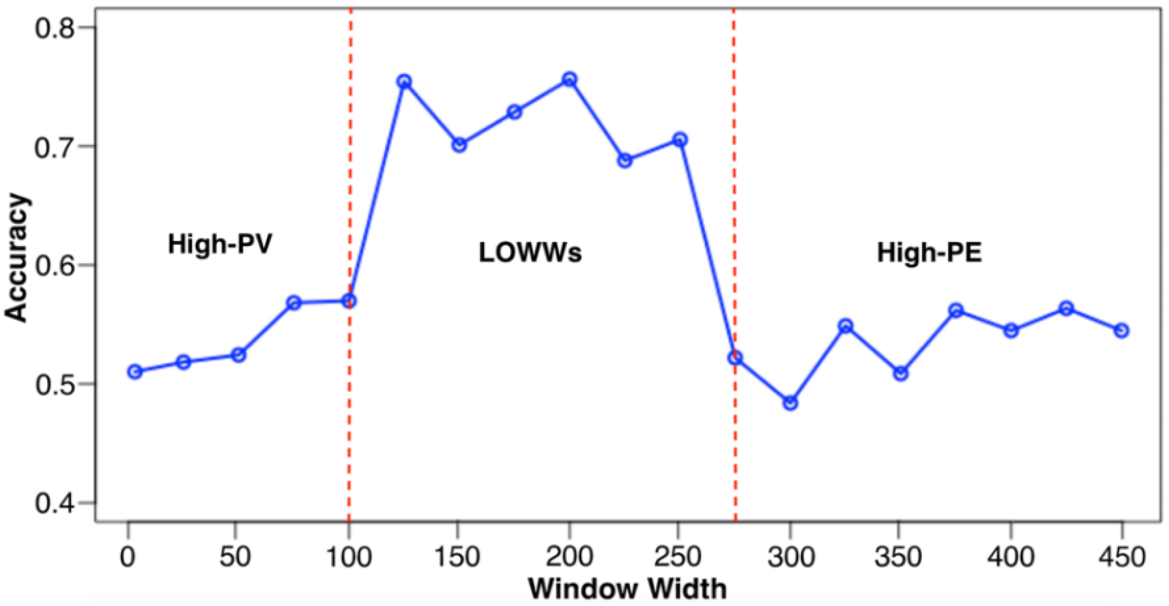
3.3. Window Width
3.4. Local Optimal Window Width
3.5. Dynamic Window
4. Methodology
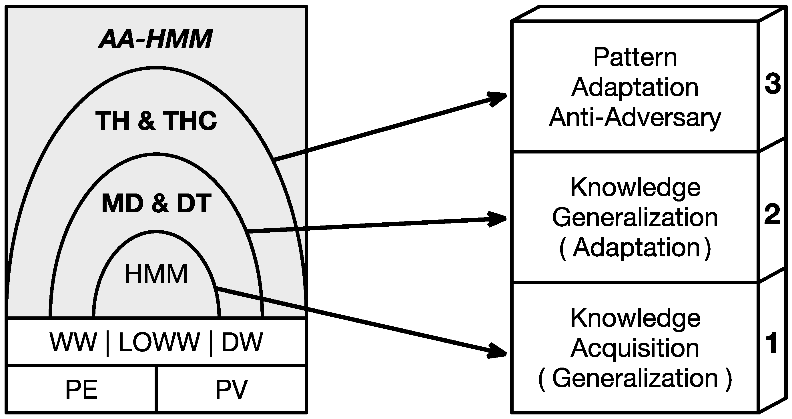
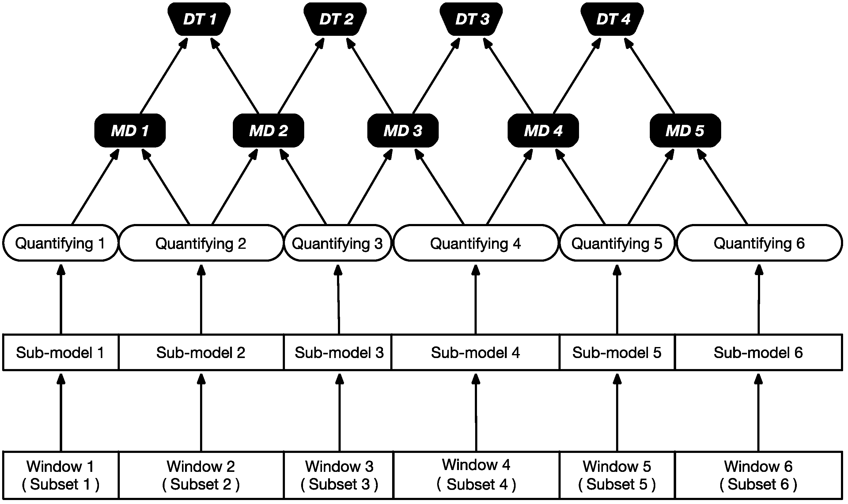
4.1. Architecture
- In order to achieve the lowest security level, the regular HMM was adopted as the base algorithm to learn the traffic pattern and make predictions.
- To attain the second security level, a pair of feedback variables, called Model Difference (MD) and Difference Trend (DT), were designed to improve the adaptability of base HMM.
- To achieve the top security level, the variable pair called Threshold (TH) and Threshold Controller (THC) were integrated to realize the required anti-adversary ability.
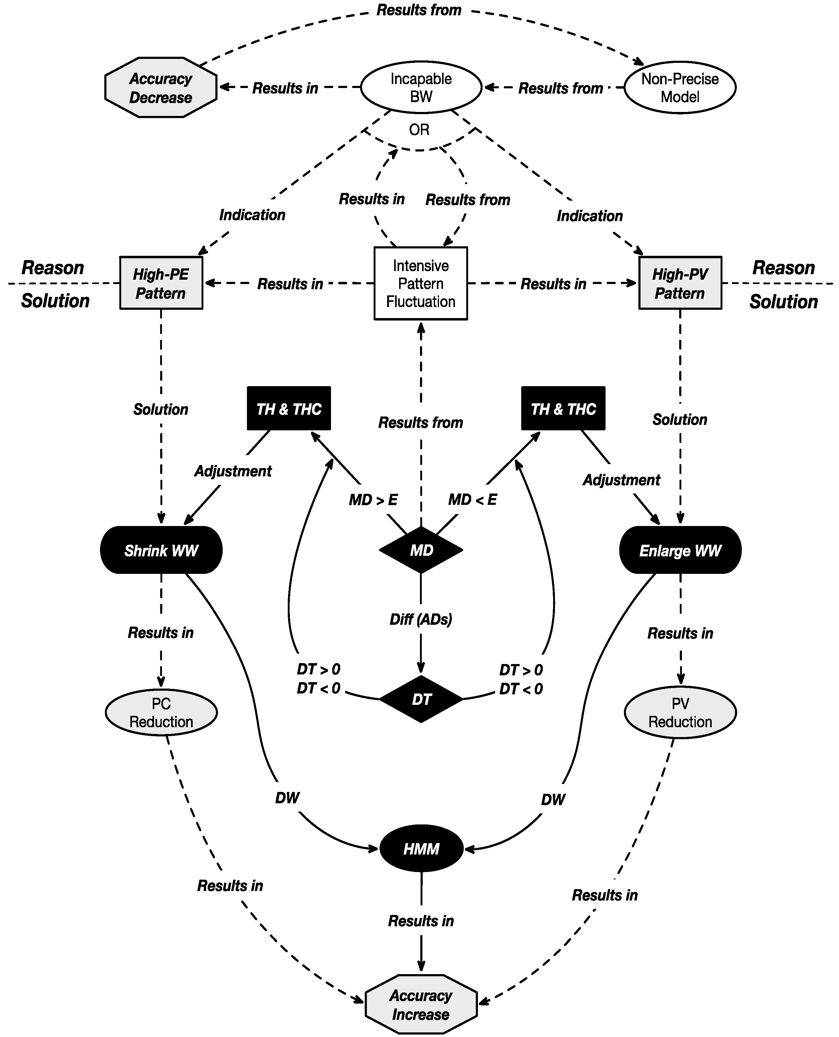
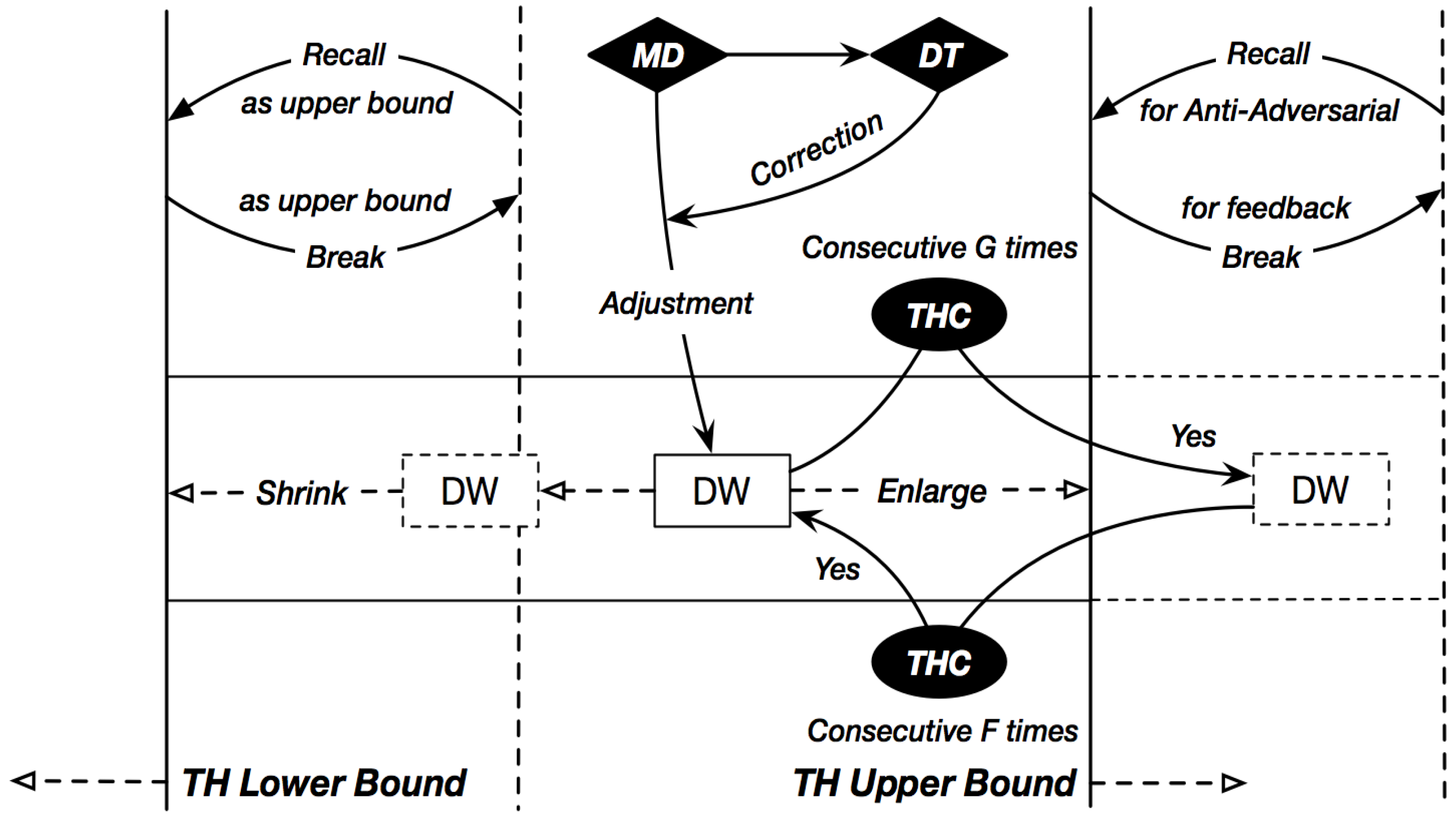
4.2. Adaptive Mechanism: MD and DT
- When MD > E, based on the difference magnitude between MD and E, the WW should be decreased to reduce the PE, then:
- ○
- If DT > 0, based on the difference magnitude between the DT and 0, the WW should be decreased again because the DT indicates that the PE of recent windows has continued to increase.
- ○
- If DT < 0, based on the difference in magnitude between the DT and 0, the WW should be increased because the DT indicates that the PE of recent windows has kept decreasing.
- When MD < E, based on the difference in magnitude between MD and E, the WW should be increased to reduce the PV, then:
- ○
- If the DT > 0, based on the difference in magnitude between DT and 0, the WW should be increased again because the DT indicates that the PV of recent windows has kept increasing.
- ○
- If DT < 0, based on the difference magnitude between the DT and 0, the WW should be decreased because the DT indicates that the PV of recent windows has kept decreasing.
4.3. Anti-Adversarial (AA) Mechanism: TH and THC
5. Implementation
5.1. Variables
5.2. Ensemble
- Even if the number of qualified sub-models is not enough for ensemble, we can build multiple dummy sub-models with varied parameters (e.g., the WW) on the same feature. Since the trajectories of different DWs would vary, the prediction results toward the same sample within different windows would be distinctive, which can be used to ensemble the result.
- Since the sub-models are working concurrently, and considering the time cost of ensemble procedure remains constant, the total time cost is only bounded by the sub-model with the highest time cost: , where the function represents the time cost of each sub-model.
5.3. Pseudocode
| AA-HMM (default setting, minor variables are omitted) |
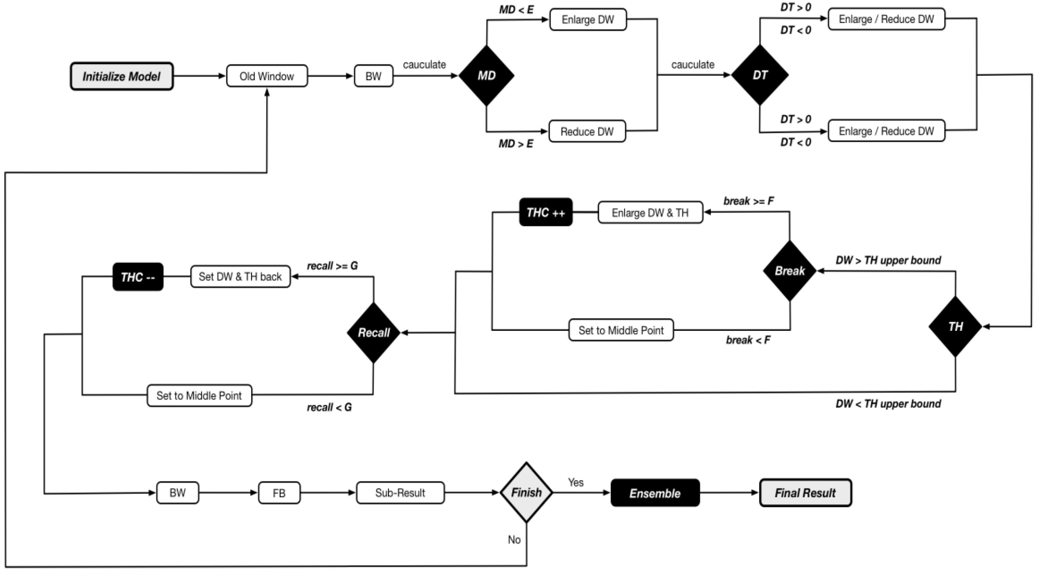
| Initial the model While (until reach the end of the data set) DW moves forward by the step of the current WW BW updates the model based on the current window Quantifying the current model Calculating Adjusting Window Width based on if MD in (0, 0.1) then WW = WW MD vector [0] else if MD in (0.1, 0.2) then WW = WW MD vector [1] else if MD in (0.2, 0.3) then WW = WW MD vector [2] …… else MD in (1, ∞) then WW = WW MD vector [10] end if Calculating Adjusting Window Width based on DT: if DT in (0, 0.1) then WW = WW DT vector_en [0] else if DT in (0.1, 0.2) then WW = WW DT vector_en [1] else if DT in (0.2, 0.3) then WW = WW DT vector_en [2] …… else DT in (1, ∞) then WW = WW DT vector_en [10] end if if DT in (−0.1, 0) then WW = WW DT vector_rd [0] else if DT in (−0.2, −0.1) then WW = WW DT vector_ rd [1] else if DT in (−0.3, 0.2) then WW = WW DT vector_ rd [2] …… else DT in (−∞, −1) then WW = WW DT vector_ rd [10] end if Adjusting WW & TH: if TH break > F + THC then new WW = {current upper bound + average [sum (intended WWs in recent F times)]}/2 new TH upper bound = {current upper bound + average [sum (intended WWs in recent F times)]/2} new TH lower bound = current lower bound + increased section of upper bound THC ++ else then new WW = (current lower bound + current upper bound)/2 end if if TH recall > G then new WW = {current lower bound − average [sum (intended WWs in recent G times)]/2} new lower bound = {current lower bound − average [sum (intended WWs in recent G times)]}/2 new upper bound = current upper bound − decreased section of lower bound THC -- else then new WW = (current lower bound + current upper bound)/2 end if BW updates the model based on the current window Quantifying the current model Calculating FW predicts the samples in DW → sub-result: End while Ensemble → majority voting among → ensemble results X |
5.4. Workflow
6. Measurement Metrics
6.1. Precision and Recall
6.2. Efficiency Matrix
7. Experiments
7.1. Goal and Strategy
7.2. Evaluation Methodology
7.2.1. Balanced Initial Model
7.2.2. Preprocessing: Compact Matrices (CM)
7.2.3. Ensemble: Assigning Different Weights
7.3. Experiment about Accuracy and Adaptivity: NSL-KDD
7.3.1. Introduction to NSL-KDD
7.3.2. Evaluation on NSL-KDD
Data Pre-Processing
Performance: Precision and Recall
Performance: Efficiency Matrix
= 8.3 + 11.25 + 65.8 + 111.3 = 196.6500
= 9.656 + 8.9373 + 66.93 + 145.5 = 231.0233
= 8.544 + 14.3925 + 93.6 + 117.615 = 234.1715
= 9.337 + 14.2965 + 93.63 + 136.59 = 253.8535
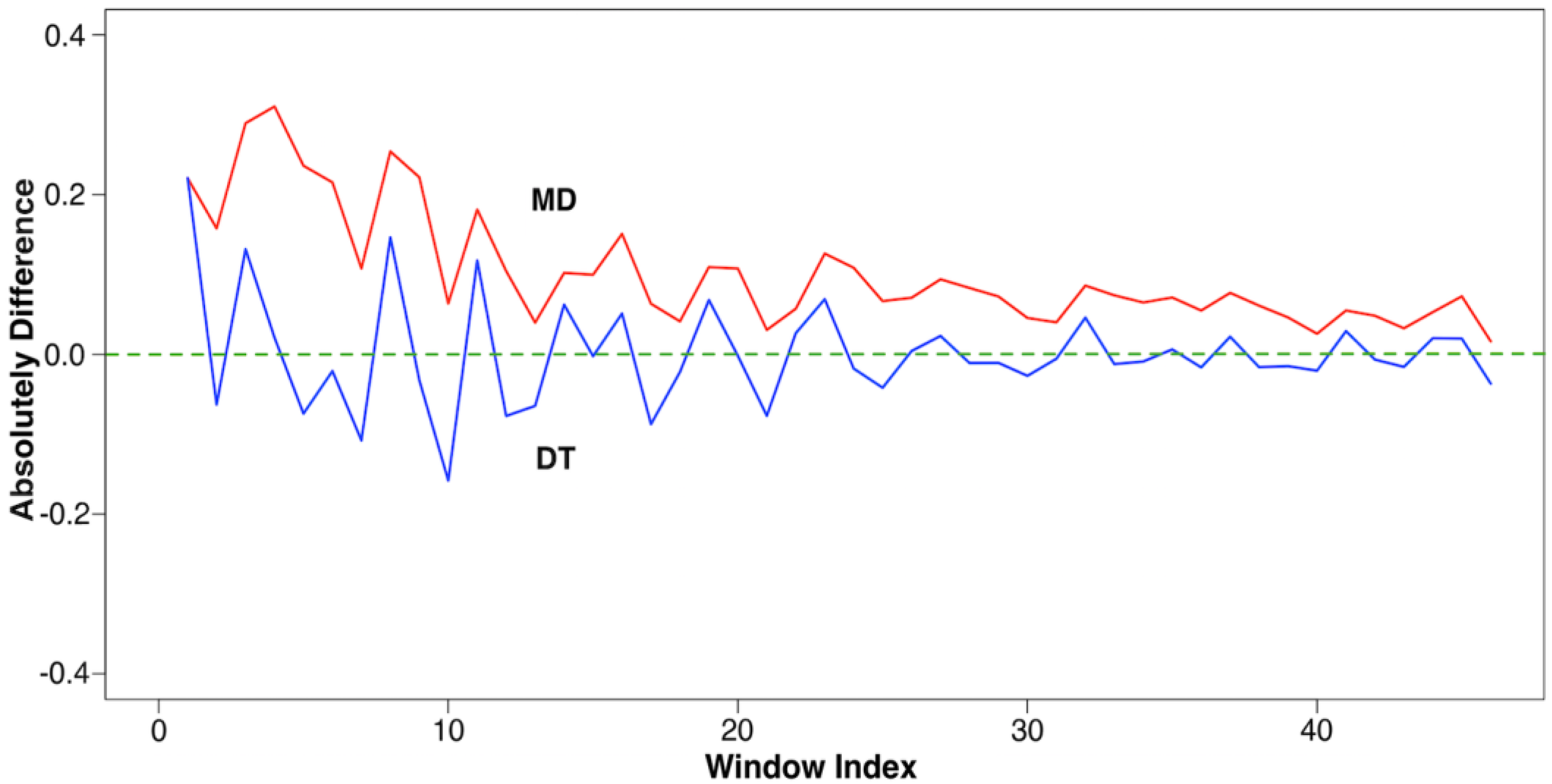
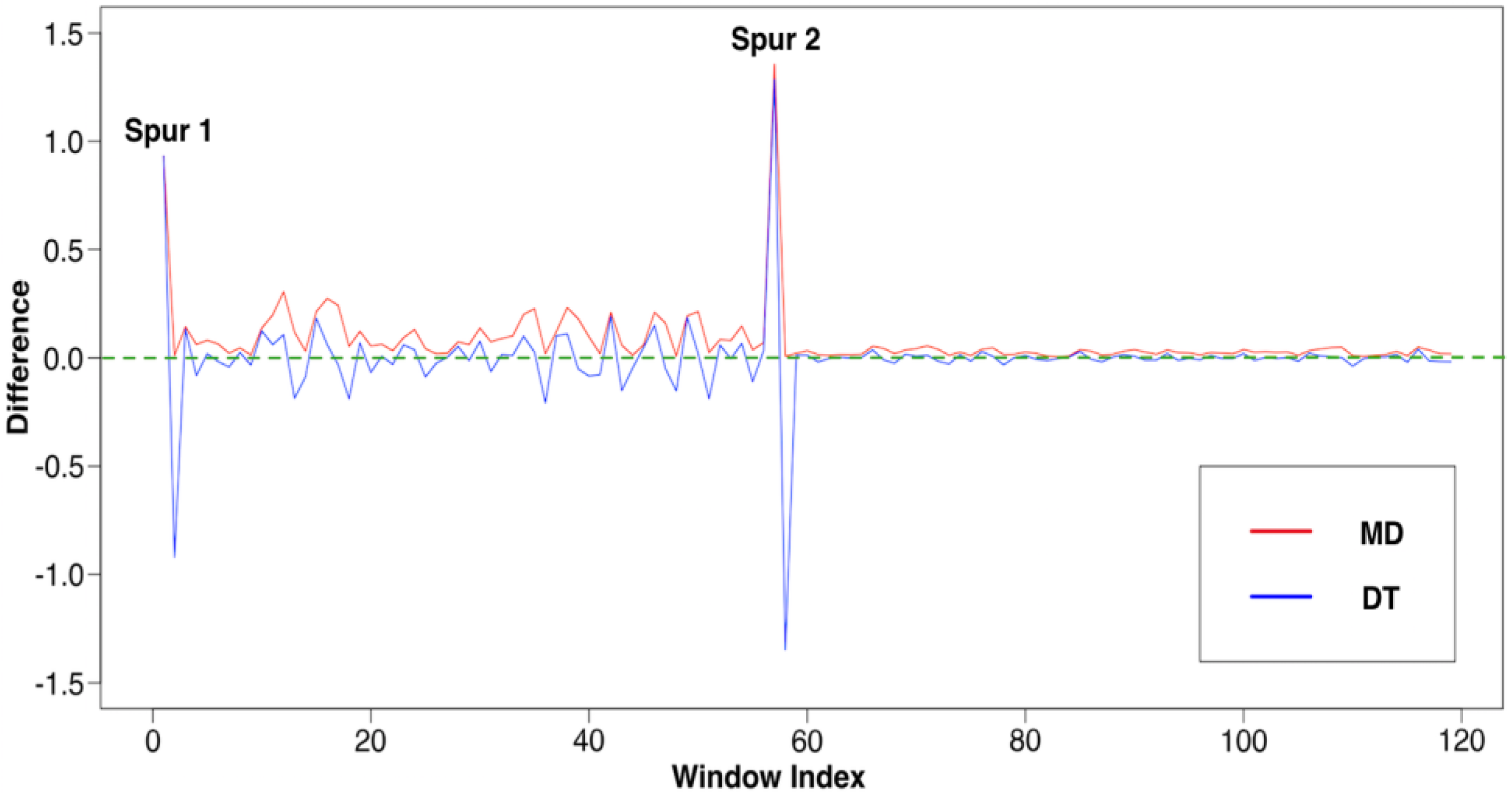
Verifications: MD and DT
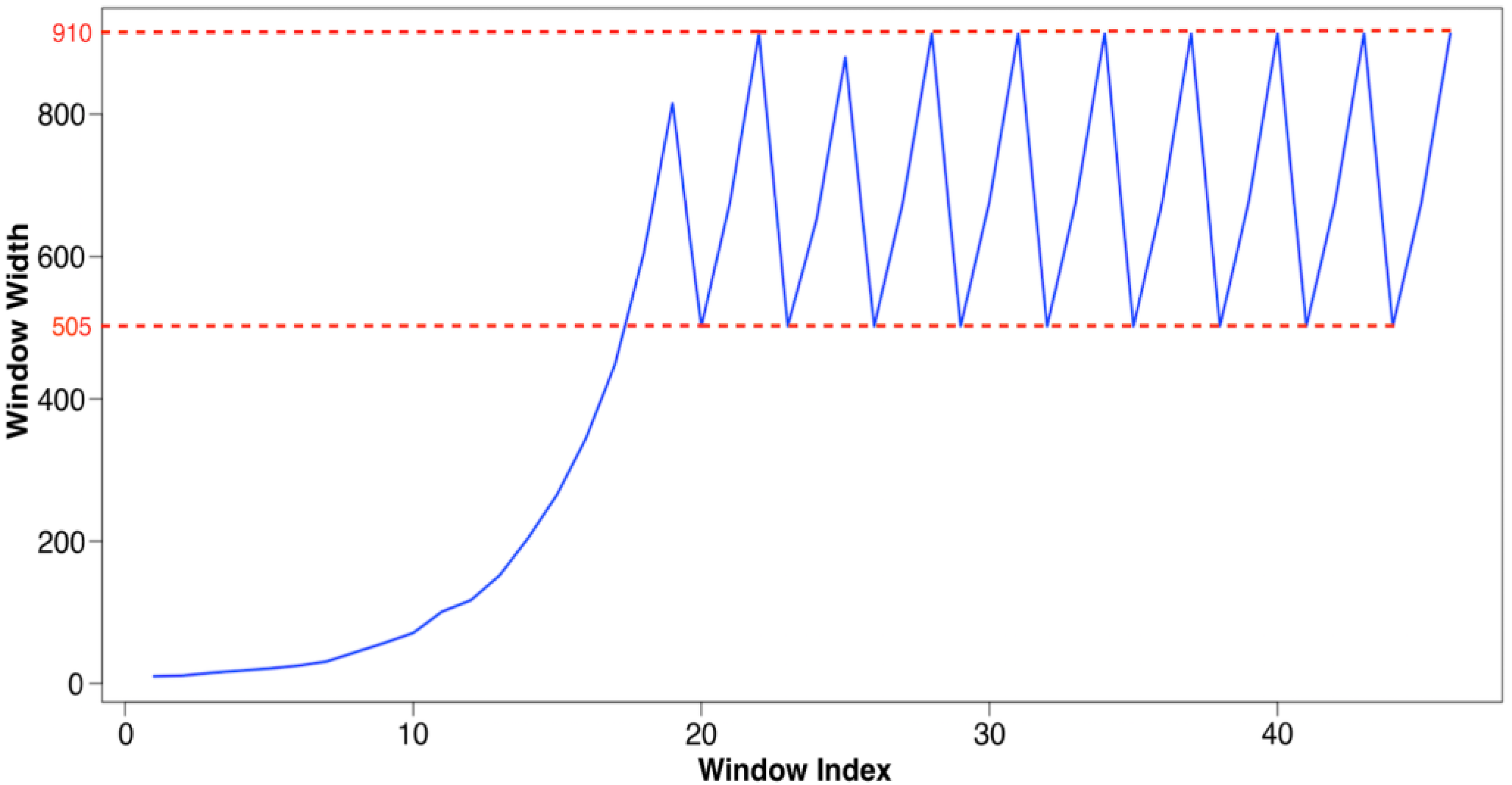
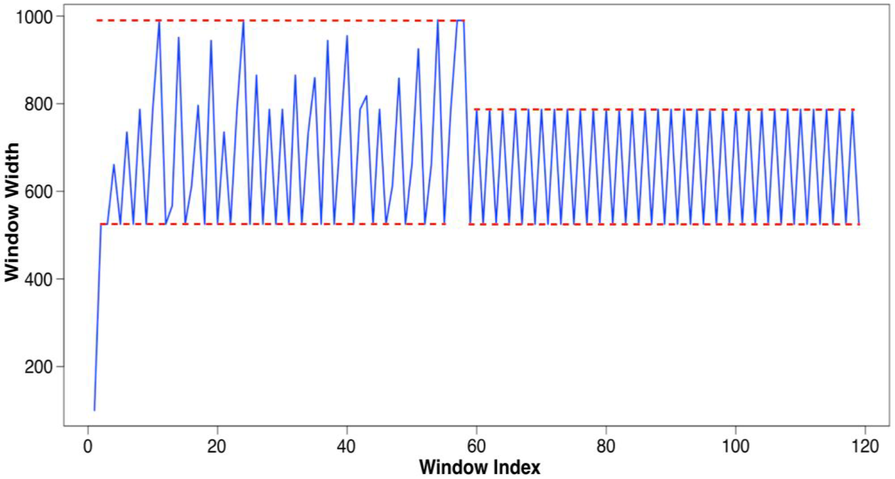
Verification: DW and TH
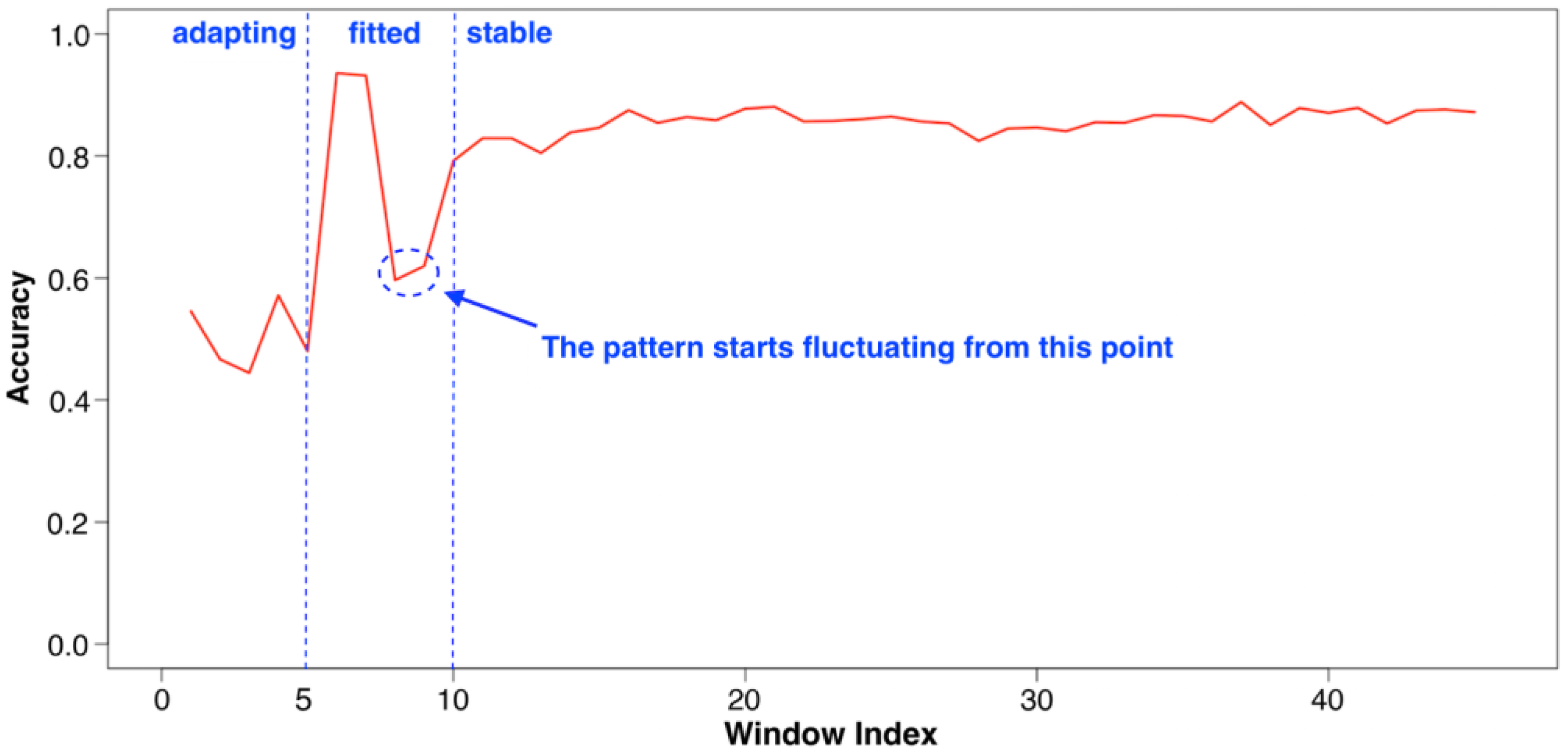
Evaluation: Adapting Rate
7.4. Anti-Adversarial Experiment: CTU-13
7.4.1. Introduction to CTU-13
7.4.2. Evaluation on CTU-13
Data Pre-Processing
Anti-Adversary and Adaptivity Performance
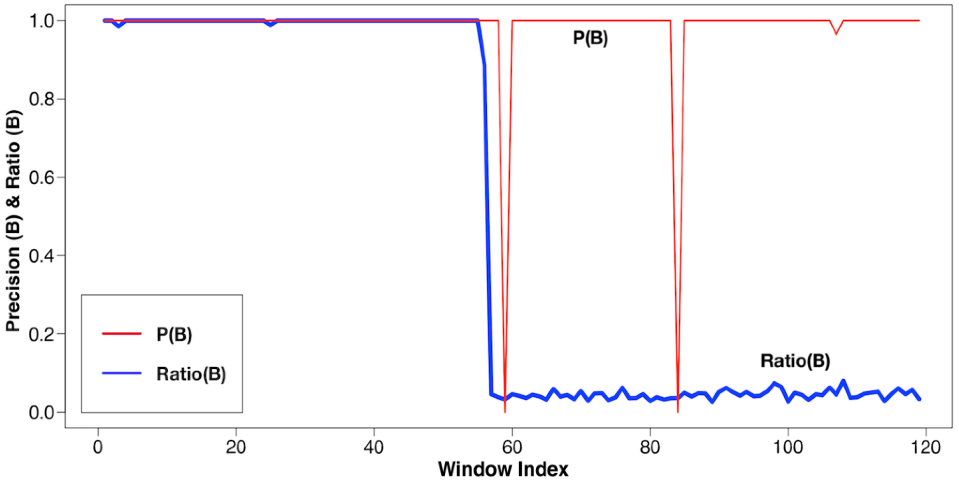
Performance: Imbalance Classes
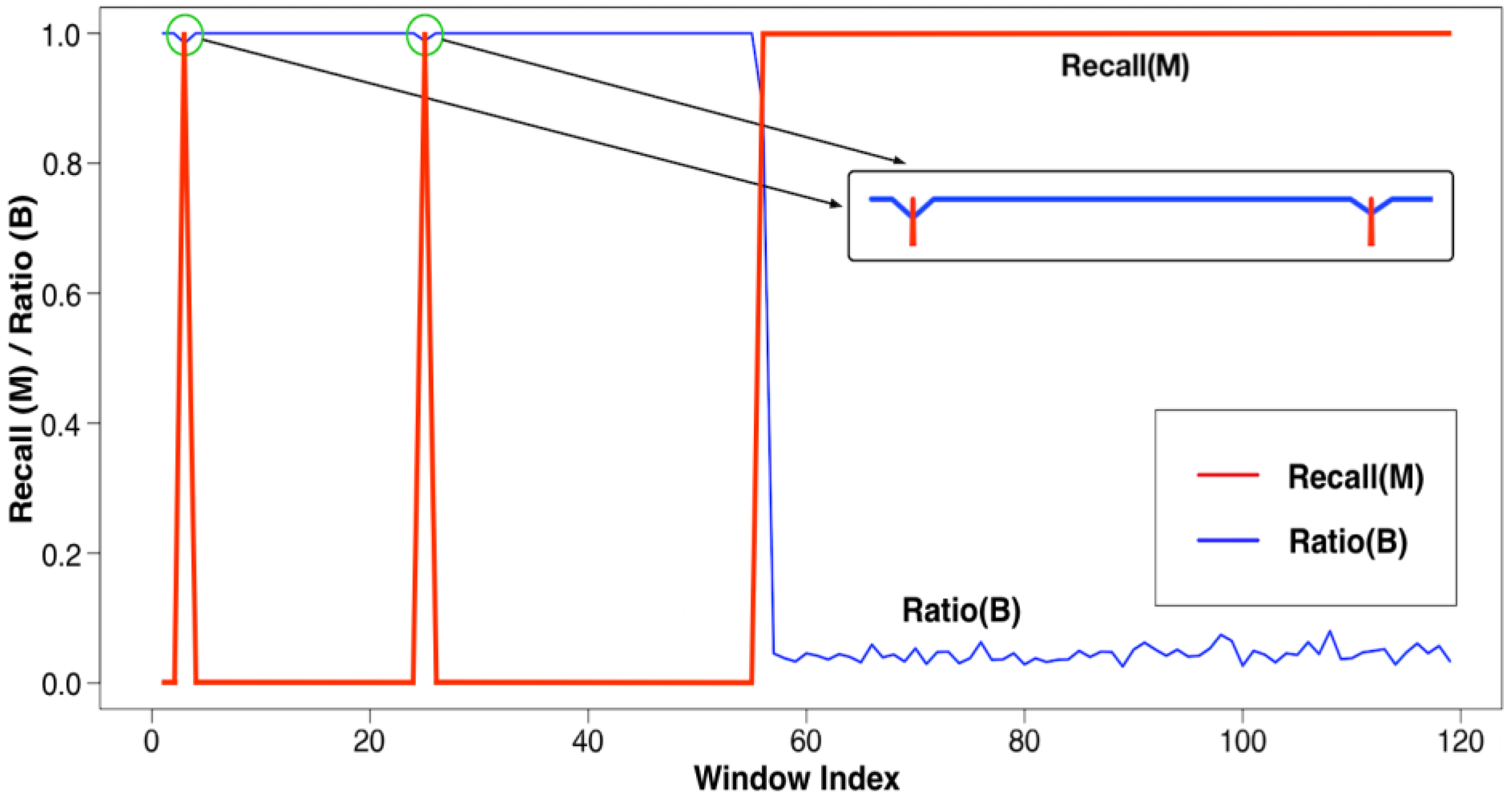
Attack Visualization
Re-Verification: MD and DT
7.5. Time Cost Experiment
8. Conclusions
Author Contributions
Funding
Conflicts of Interest
Abbreviations
| AA-HMM | Anti-Adversarial Hidden Markov Model |
| B | benign (samples) |
| BM | Balance Model |
| BW | Baum-Welch |
| CM | Compact Matrix |
| DDoS | Distributed Denial-Of-Service |
| DNN | Deep neural network |
| DT | Difference Trend |
| DW | Dynamic Window |
| EM | Efficiency Matrix |
| FB | Forward-Backward |
| HMM | Hidden Markov Model |
| LDA | Linear Discriminant Analysis |
| LOWW | Local Optimal Window Width |
| M | Malicious (samples) |
| MD | Model Difference |
| ML | Machine Learning |
| NIDS | Network Intrusion Detection System |
| OE | Optimal Evasion |
| PCA | Principal Component Analysis |
| PE | Pattern Entropy |
| PERD | PE ReDuction |
| PV | Pattern Variation |
| ROC curve | Receiver Operating Characteristic curve |
| SMR | Soft-Max Regression |
| STL | Self-Taught Learning |
| TH | Threshold |
| THC | Threshold Controller |
| TTC | Total Time Cost |
| WW | Window Width |
References
- Sommer, R.; Paxson, V. Outside the Closed World—On Using Machine Learning for Network Intrusion Detection. In Proceedings of the IEEE Symposium on Security and Privacy, Berkeley/Oakland, CA, USA, 16–19 May 2010. [Google Scholar]
- Linden, G.; Smith, B.; York, J. Amazon.com recommendations: Item-to-item collaborative filtering. IEEE Internet Comput. 2003, 7, 76–80. [Google Scholar] [CrossRef]
- Gomez-Uribe, C.A.; Hunt, N. The Netflix Recommender System: Algorithms, Business Value, and Innovation. ACM Trans. Manag. Inf. Syst. 2016, 6, 13. [Google Scholar] [CrossRef]
- Khan, N.H.; Adnan, A. Urdu Optical Character Recognition Systems: Present Contributions and Future Directions. IEEE Access 2018, 6, 46019–46046. [Google Scholar] [CrossRef]
- Chen, K.; Zhao, T.; Yang, M.; Liu, L.; Tamura, A.; Wang, R.; Utiyama, M.; Sumita, E. A Neural Approach to Source Dependence Based Context Model for Statistical Machine Translation. IEEE Access 2018, 6, 266–280. [Google Scholar] [CrossRef]
- Hsia, J.H.; Chen, M.S. Language-model-based detection cascade for efficient classification of image-based spam e-mail. In Proceedings of the 2009 IEEE international conference on Multimedia and Expo ICME’09, New York, NY, USA, 28 June–3 July 2009; pp. 1182–1185. [Google Scholar]
- Zhang, F.; Chan, P.P.; Biggio, B.; Yeung, D.S.; Roli, F. Adversarial Feature Selection Against Evasion Attacks. IEEE Trans. Cybern. 2016, 46, 766–777. [Google Scholar] [CrossRef] [PubMed]
- Polychronakis, M.; Anagnostakis, K.G.; Markatos, E.P. Real-world Polymorphic Attack Detection using Network-level Emulation. In Proceedings of the 4th Annual Workshop on Cyber Security and Information Intelligence Research: Developing Strategies to Meet the Cyber Security and Information Intelligence Challenges Ahead, Oak Ridge, TN, USA, 12–14 May 2008. [Google Scholar]
- Kaur, H.; Singh, G.; Minhas, J. A Review of Machine Learning based Anomaly Detection Techniques. Int. J. Comput. Appl. Technol. Res. 2013, 2, 185–187. [Google Scholar] [CrossRef]
- Bhuyan, M.H.; Bhattacharyya, D.K.; Kalita, J.K. Network Anomaly Detection: Methods, Systems and Tools. IEEE Commun. Surv. Tutor. 2014, 16, 303–336. [Google Scholar] [CrossRef]
- Kuncheva, L.I. Combining Pattern Classifiers: Methods and Algorithms; Wiley: Hoboken, NJ, USA, 2004. [Google Scholar]
- Kuncheva, L.I. Diversity in multiple classifier systems. Inf. Fusion 2005, 6, 3–4. [Google Scholar] [CrossRef]
- Weng, F.; Jiang, Q.; Shi, L.; Wu, N. An Intrusion Detection System Based on the Clustering Ensemble. In Proceedings of the International Workshop on Anti-Counterfeiting, Security and Identification (ASID), Xiamen, China, 16–18 April 2007; pp. 121–124. [Google Scholar]
- Hodo, E.; Bellekens, X.; Hamilton, A.; Tachtatzis, C.; Atkinson, R. Shallow and Deep Networks Intrusion Detection System: A Taxonomy and Survey. arXiv, 2017; arXiv:1701.02145. [Google Scholar]
- Shankar, V.; Chang, S. Performance of Caffe on QCT Deep Learning Reference Architecture—A Preliminary Case Study. In Proceedings of the IEEE 4th International Conference on Cyber Security and Cloud Computing (CSCloud), New York, NY, USA, 26–28 June 2017; pp. 35–39. [Google Scholar]
- Khreich, W.; Granger, E.; Sabourin, R.; Miri, A. Combining Hidden Markov Models for Improved Anomaly Detection. In Proceedings of the IEEE International Conference on Communications, Dresden, Germany, 14–18 June 2009; pp. 1–6. [Google Scholar]
- Hu, J.; Yu, X.; Qiu, D.; Chen, H.H. A simple and efficient hidden Markov model scheme for host-based anomaly intrusion detection. IEEE Netw. 2009, 23, 42–47. [Google Scholar] [CrossRef]
- Hurley, T.; Perdomo, J.E.; Perez-Pons, A. HMM-Based Intrusion Detection System for Software Defined Networking. In Proceedings of the 15th IEEE International Conference on Machine Learning and Applications (ICMLA), Anaheim, CA, USA, 18–20 December 2016; pp. 617–621. [Google Scholar]
- Jain, R.; Abouzakhar, N.S. Hidden Markov Model based anomaly intrusion detection. In Proceedings of the International Conference for Internet Technology and Secured Transactions, London, UK, 10–12 December 2012; pp. 528–533. [Google Scholar]
- Song, X.; Chen, G.; Li, X. A Weak Hidden Markov Model based intrusion detection method for wireless sensor networks. In Proceedings of the International Conference on Intelligent Computing and Integrated Systems, Guilin, China, 22–24 October 2010; pp. 887–889. [Google Scholar]
- Ren, H.; Ye, Z.; Li, Z. Anomaly detection based on a dynamic Markov model. Inf. Sci. 2017, 411, 52–65. [Google Scholar] [CrossRef]
- Ahmadian, R.A.; Rasoolzadegan, A.; Javan, J.A. A systematic review on intrusion detection based on the Hidden Markov Model. Stat. Anal. Data Min. ASA Data Sci. J. 2018, 11, 111–134. [Google Scholar] [CrossRef]
- Ariu, D.; Tronci, R.; Giacinto, G. HMMPayl: An intrusion detection system based on Hidden Markov Model. Comput. Secur. 2011, 30, 221–241. [Google Scholar] [CrossRef]
- Russell, S.J.; Norvig, P. Artificial Intelligence: A Modern Approach, 3rd ed.; Pearson: Kuala Lumpur, Malaysia, 2009. [Google Scholar]
- Tan, P.N.; Steinbach, M.; Kumar, V. Introduction to Data Mining; Pearson: London, UK, 2006. [Google Scholar]
- Rabiner, L.R. A Tutorial on Hidden Markov Model and Selected Applications in Speech Recognition. Proc. IEEE 1989, 77, 257–286. [Google Scholar] [CrossRef]
- Zhao, F.; Zhao, J.; Niu, X.; Luo, S.; Xin, Y. A Filter Feature Selection Algorithm Based on Mutual Information for Intrusion Detection. Appl. Sci. 2018, 8, 1535. [Google Scholar] [CrossRef]
- Hindy, H.; Brosset, D.; Bayne, E.; Seeam, A.; Tachtatzis, C.; Atkinson, R.; Bellekens, X. A Taxonomy and Survey of Intrusion Detection System Design Techniques, Network Threats and Datasets. arXiv, 2018; arXiv:1806.03517. [Google Scholar]
- The R Project for Statistical Computing. Available online: https://cran.r-project.org/web/packages/HMM/HMM.pdf (accessed on 11 October 2018).
- Lowd, D.; Meek, C. Adversarial learning. In Proceedings of the Eleventh ACM SIGKDD International Conference on Knowledge Discovery in Data Mining, Chicago, IL, USA, 21–24 August 200; pp. 641–647.
- Nelson, B.; Rubinstein, B.I.; Huang, L.; Joseph, A.D.; Lee, S.J.; Rao, S.; Tygar, J.D. Query strategies for evading convex-inducing classifiers. J. Mach. Learn. Res. 2012, 13, 1293–1332. [Google Scholar]
- Churbanov, A.; Winters-Hilt, S. Implementing EM and Viterbi algorithms for Hidden Markov Model in linear memory. BMC Bioinform. 2008, 9, 224. [Google Scholar] [CrossRef] [PubMed]
- McHugh, J. Testing Intrusion Detection Systems: A Critique of the 1998 and 1999 DARPA Intrusion Detection System Evaluations as Performed by Lincoln Laboratory. ACM Trans. Inf. Syst. Secur. 2000, 3, 262–294. [Google Scholar] [CrossRef]
- Canadian Institute for Cybersecurity. Available online: http://www.unb.ca/cic/datasets/nsl.html (accessed on 11 October 2018).
- Tang, T.A.; Mhamdi, L.; McLernon, D.; Zaidi, S.A.R.; Ghogho, M. Deep Learning Approach for Network Intrusion Detection in Software Defined Networking. In Proceedings of the International Conference on Wireless Networks and Mobile Communications (WINCOM), Fez, Morocco, 26–29 October 2016. [Google Scholar]
- Niyaz, Q.; Sun, W.; Javaid, A.Y.; Alam, M. A Deep Learning Approach for Network Intrusion Detection System. In Proceedings of the 9th EAI International Conference on Bio-inspired Information and Communications Technologies, BICT’15, New York, NY, USA, 3–5 December 2015; pp. 21–26. [Google Scholar]
- Garcia, S.; Grill, M.; Stiborek, J.; Zunino, A. An empirical comparison of botnet detection methods. Comput. Secur. J. 2014, 45, 100–123. [Google Scholar] [CrossRef]
- Dhanabal, L.; Shantharajah, S.P. A Study on NSL-KDD Data set for Intrusion Detection System Based on Classification Algorithms. Int. J. Adv. Res. Comput. Commun. Eng. 2015, 4, 446–452. [Google Scholar]
- Song, C.; Perez-Pons, A.; Yen, K.K. Building a Platform for Software-Defined Networking Cybersecurity Applications. In Proceedings of the 15th IEEE International Conference on Machine Learning and Applications (ICMLA), Anaheim, CA, USA, 18–20 December 2016; pp. 482–487. [Google Scholar]


| Name | Description | Default Value |
|---|---|---|
| window width | width of the dynamic window | 10 |
| window base line | minimum width of the dynamic window | 10 |
| threshold lower bound | lower bound of the dynamic window | 10 |
| threshold upper bound | upper bound of the dynamic window | 1000 |
| threshold break | a counter that records the number of consecutive requests of increasing the threshold upper bound | starts from 0 |
| F | threshold for increasing the upper bound | 3 |
| threshold recall | a counter that records the number of consecutive times of the increased section of threshold has not been used | starts from 0 |
| G | threshold for recall the increased upper bound | 3 |
| threshold controller | controlling the difficulty of threshold adjustment | 0 |
| MD vector | levels of resizing the window based on the MD | from 1.5 to 0.5 step by −0.1 |
| DT vector_en | he levels of enlarging the window based on the DT | from 1 to 1.2 step by 0.02 |
| DT vector_sh | levels of reducing the window based on the DT | from 1 to 0.8 step by −0.02 |
| levels | graininess of WW adjustment for MD and DT | from 0 to 1 step by 0.1 |
| Efficiency Matrix | Precision | Recall |
|---|---|---|
| Benign | ||
| Malicious |
| Transition | Benign | Malicious |
|---|---|---|
| Benign | 0.5 | 0.5 |
| Malicious | 0.5 | 0.5 |
| Emission | Observation 1 | Observation 2 | … | Observation n |
|---|---|---|---|---|
| Benign | 0.5 | 0.5 | … | 0.5 |
| Malicious | 0.5 | 0.5 | … | 0.5 |
| DNN | Precision | Recall | Accuracy |
|---|---|---|---|
| Benign | 83.00% | 75.00% | 74.67% |
| Malicious | 65.80% | 74.20% |
| SMR | Precision | Recall | Accuracy |
|---|---|---|---|
| Benign | 96.56% | 63.73% | 78.06% |
| Malicious | 66.93% | 97.00% |
| STL | Precision | Recall | Accuracy |
|---|---|---|---|
| Benign | 85.44% | 95.95% | 88.39% |
| Malicious | 93.62% | 78.41% |
| AA-HMM | Precision | Recall | Accuracy |
|---|---|---|---|
| Benign | 93.37% | 95.31% | 93.48% |
| Malicious | 93.63% | 91.06% |
| Efficiency Matrix | Precision | Recall |
|---|---|---|
| Benign | 10 | 15 |
| Malicious | 100 | 150 |
© 2018 by the authors. Licensee MDPI, Basel, Switzerland. This article is an open access article distributed under the terms and conditions of the Creative Commons Attribution (CC BY) license (http://creativecommons.org/licenses/by/4.0/).
Share and Cite
Song, C.; Pons, A.; Yen, K. AA-HMM: An Anti-Adversarial Hidden Markov Model for Network-Based Intrusion Detection. Appl. Sci. 2018, 8, 2421. https://doi.org/10.3390/app8122421
Song C, Pons A, Yen K. AA-HMM: An Anti-Adversarial Hidden Markov Model for Network-Based Intrusion Detection. Applied Sciences. 2018; 8(12):2421. https://doi.org/10.3390/app8122421
Chicago/Turabian StyleSong, Chongya, Alexander Pons, and Kang Yen. 2018. "AA-HMM: An Anti-Adversarial Hidden Markov Model for Network-Based Intrusion Detection" Applied Sciences 8, no. 12: 2421. https://doi.org/10.3390/app8122421
APA StyleSong, C., Pons, A., & Yen, K. (2018). AA-HMM: An Anti-Adversarial Hidden Markov Model for Network-Based Intrusion Detection. Applied Sciences, 8(12), 2421. https://doi.org/10.3390/app8122421