Abstract
Kidney cancer is one of the deadliest diseases and its diagnosis and subtype classification are crucial for patients’ survival. Thus, developing automated tools that can accurately determine kidney cancer subtypes is an urgent challenge. It has been confirmed by researchers in the biomedical field that miRNA dysregulation can cause cancer. In this paper, we propose a machine learning approach for the classification of kidney cancer subtypes using miRNA genome data. Through empirical studies we found 35 miRNAs that possess distinct key features that aid in kidney cancer subtype diagnosis. In the proposed method, Neighbourhood Component Analysis (NCA) is employed to extract discriminative features from miRNAs and Long Short Term Memory (LSTM), a type of Recurrent Neural Network, is adopted to classify a given miRNA sample into kidney cancer subtypes. In the literature, only a couple of kidney subtypes have been considered for classification. In the experimental study, we used the miRNA quantitative read counts data, which was provided by The Cancer Genome Atlas data repository (TCGA). The NCA procedure selected 35 of the most discriminative miRNAs. With this subset of miRNAs, the LSTM algorithm was able to group kidney cancer miRNAs into five subtypes with average accuracy around 95% and Matthews Correlation Coefficient value around 0.92 under 10 runs of randomly grouped 5-fold cross-validation, which were very close to the average performance of using all miRNAs for classification.
1. Introduction
Kidney cancer is one of the deadliest diseases and unfortunately it is hard to detect early through normal clinical means [1]. Despite being one of the top-ten killer-cancers, there is a lack of research effort on kidney cancer. It has been overshadowed by other cancer types in the medical community, which has hindered the development of new techniques to detect and treat it. For decades, patients with kidney cancer have had limited options of treatment beyond surgery, and in most cases, life expectancy is less than one year. Thus, it is crucial to detect the disease early. Besides traditional clinical techniques, the study of various biomarkers brings researchers closer to understanding the onset of kidney cancer, making accurate diagnoses, and removing the ambiguity surrounding this disease. However, even with all the genomic understanding and technological progress, there are many unclear answers and undiscovered paths of research. Researchers need to explore new techniques to detect this disease and diagnose both the stage and sub-type accurately, thus assisting physicians in prescribing the right treatment options to each distinguished case while reducing the undesired harmful side-effects of drugs and increasing the survival rate of patients.
Recently, various efforts have been developed to differentiate among sub-types of kidney cancer. One of these promising paths is the analysis of the genetic information of the patient. Clinical diagnosis through miRNA expression has enticed a significant amount of researchers, especially since the technological revolution of miRNA information extraction during the last two decades. One of the foremost sources of data for genetic information of various cancers is furnished by The Cancer Genome Atlas (TCGA), which is a product of the collaboration between the National Cancer Institute (NCI) and the National Human Genome Research Institute (NHGRI). This platform has generated comprehensive multi-dimensional maps of the key genomic changes in the 33 types of cancers [2], including kidney cancer.
In this study, we focus on kidney cancer sub-type detection and classification in an effort to assist researchers in medicine to address the key points of kidney subtypes and their characteristics. Many studies have shown strong relationships between cancer types and variations in miRNA regulation. In this study, we utilize the variation in miRNAs due to the difference in miRNA up-regulation and down-regulation among the kidney cancer subtypes and consider it as the main attribute to perform this differentiation. With the proposed method, we were able to select high weighted features that led us to obtain 35 miRNAs, which were extracted from a total of 1881 identified by the TCGA dataset for kidney cancer. By performing a deep training procedure, we were able to distinguish the five kidney cancer sub-types in the TCGA and TARGET projects dispensed by the TCGA repository.
More specifically, we use Neighborhood Component Analysis (NCA) [3] as a feature selection algorithm to find the most discriminative miRNAs for each subtype. The selected miRNAs are fed to a classifier to determine the exact kidney subtype. The adopted classification method is a type of Recurrent Neural Network, Long Short-Term Memory (LSTM) [4,5], which is a machine learning tool that deals with sequential and non-sequential data signals. To assess the performance of the proposed method, we adopted the Data Analysis Protocol and the Matthews Correlation Coefficient [6]. It has to be stressed, however, that the effectiveness of the selected miRNA subset for diagnosing specific subtypes of kidney needs to be investigated clinically.
The rest of the paper is organized in the following manner: Section 2 discusses the relationship between miRNA-sequence and cancer in general and kidney cancer in particular. Section 3 gives a summary of the tools used in this study, i.e., the Neighborhood Component Analysis procedure and the Long Short-Term Memory algorithm. Section 4 outlines the adopted data preparation and assessment process. It then provides the classification results with discussions. Conclusions are given in Section 5.
2. The RNA Sequence and Kidney Cancer
MiRNA is a small non-coding RNA, and its length is approximately 19–25 nucleotides, which is relatively short. It has considerable biological importance at the molecular level and acts to control the miRNAs post-transcriptionally in plants, animals, and some viruses. In the human genome, there are thousands of classified miRNAs and they are responsible for targeting about 60% of protein-coding [7,8]. MiRNA plays an important role in basic biological processes inside our bodies such as proliferation, cell cycle control, apoptosis, differentiation, migration, and metabolism. Although many features of the miRNA biogenesis conduct are still hazy, the key processes have been characterized. MiRNA dysregulation can result in numerous types of cancers. Microarray expression data collected from a wide range of cancers have since proved that aberrant miRNA is the initial factor that influences cancer [9,10,11,12,13]. Recent studies on mouse strains have shown that individual miRNAs or miRNA clusters are responsible for a range of diseases. It has been stated that low levels of mature miRNAs are linked to cancerous diseases [10] and miRNAs have been proven to be among the most promising biomarkers for providing information about cancer sub-type differentiation and prognosis [14]. For more details and an understanding of the miRNA and cancer correlation, please refer to [9].
Researchers are seeking to address the significant miRNA bio-factors and to identify the exact miRNAs with the greatest discriminative power as biomarkers which precise diagnosis depends on, especially for the task of identifying kidney cancer sub-types and staging. The following summarizes some of these research efforts done in this field to help understand the relationship between miRNA and kidney cancer sub-types and staging identification. White et al. [15] performed combinatorial analysis on previously reported dysregulated miRNAs and identified 62 miRNAs out of the 133 miRNAs previously reported by other researchers. In [16], 35 miRNAs were found to distinguish between clear cell Renal Cell Carcinoma (ccRCC) and patient-matched normal kidney tissue. Among this group of 35 miRNA, nine were up-regulated and 26 were down-regulated and miRNA 106b was selected as the reference point as endogenous control. Samaan et al. [17] reported that over-expressed levels of miR-210 were found in ccRCC with higher levels of expression in metastatic tumors, where high expression was considered as an independent biomarker of poor prognosis in ccRCC. Higher levels noticed in the clear cell and papillary sub-types compared with chromophobe renal cell carcinoma and oncocytoma. In [18], the authors stated that significantly higher expression levels of exosomal miR-210 and miR-1233 were found in ccRCC patients than in healthy samples. A combined expression level of miR-21 and miR-126 can be used to predict cancer-specific survival in two independent RCC groups depending on the sensitivity of the up-regulation of the mir-21 and down-regulation of mir-126 [19]. Studies reported in [20] showed that the up-regulation of the miR-21 was correlated with clinical characteristics of renal cancer which led to lowering kidney cancer survival time.
From these studies, the reader can deduce that there is a level of uncertainty among the researchers’ claims that a specific group of miRNAs is the best candidate to differentiate among the sub-types or has a significant role in detection. Wach et al. [21] performed micro-array analysis and stated that RCC was a variety of different entities, each having a distinguishable molecular pattern. The high similarity in miRNA expression was observed between matched tumor and normal tissue taken from the same RCC case. Recent studies tried to understand the linkage between RCC tumors or tumor entities and miRNAs. White et al. [22] used 35 miRNAs in a cluster analysis to discriminate between the corresponding pairs of the ccRCC and normal samples. In [23], the authors addressed several pairs of miRNAs that have the capability to differentiate between RCC cases of different entities and a normal sample, they achieved a distinguishing sensitivity of 97% using a vote counting strategy. However, in [21], over 86% accuracy was achieved using only four sets of miRNAs that can be used to distinguish between tumor samples of different RCC entities and normal ones. In [24], a group of nine primary transcripts and 18 mature miRNAs were listed as the differential expression of 27 miRNAs, while [21] claims that only 10 of the 18 mature miRNAs can be used as differential expression according to his analysis. By using vote-counting strategy, 28 miRNAs were able to classify tumor samples into ccRCC, chromophobe RCC, pRCC, or oncocytoma with 87% accuracy. To classify between ccRCC and pRCC, they presented a binary classification system using only 11 miRNAs [23].
It can be seen that most researchers focused on limited groups of miRNAs, or on a specific subtype of kidney cancer. In our research, we consider the entire set of 1881 miRNAs, excluding only the null quantities to obtain a final subset of 1627 miRNAs. We selected the 35 isolated miRNAs using the feature selection tool which will be discussed in Section 3.1. In addition, we will consider five sub-types as categorized by the TCGA and TARGET kidney cancer projects.
3. Machine Learning
A typical machine learning algorithm starts with feature selection, though deep learning algorithms can also be designed to handle raw data [25,26]. With regard to feature selection, it was demonstrated in [3] that NCA is an effective method for selecting significant feature points for high-dimensional data. This method is a nearest neighbor-based feature weighting algorithm. As a feature selection tool, the NCA method was successfully tested on several microarray datasets for various cancers, such as colon cancer, brain tumor, leukemia, lung cancer, and prostate cancer [3]. In this research, we adopt the NCA algorithm for selecting high-rank features form miRNA data.
Another important tool in automated cancer subtype classification is an effective classifier. In the literature [27], various deep learning techniques were used for this purpose. For instance, LSTM networks were used for Pulmonary Nodule Detection given CT Images, illustrating a significant discriminative capability [28]. Similarly, a three-layered 1D LSTM network was trained for extracting prognostic information of colorectal cancer from tissue images [29]. In [30], a segmentation algorithm based on deep-learning was presented for the identification of pathological kidneys in CT images. In this paper, we will explore the efficacy of LSTM networks for kidney cancer subtype classification.
Brief descriptions of the NCA method and LSTM network are given in the following subsections.
3.1. Neighborhood Component Analysis
Let us consider kidney sub-type classification, a multi-class classification problem. Let c be the number of subtype classes, and n the number of observations (patients). Then a given training set can be described as follows [3]:
where are the feature vectors, and are the class labels. Let be the classifier to be trained.
Consider a randomized classifier that picks a reference point randomly, , then labels x using the label of the randomly selected reference point . By choosing the reference point to be the nearest neighbor of the given point x, one makes the algorithm similar to that of the Nearest Neighbor Classifier. However, in the NCA algorithm, the choice of the reference point is based on some probability, which is called the selection probability. The probability will be higher if the reference point of x, , is closer to x, as measured by the distance function .
Where for are the feature weights. Assume that the selection probability is direct proportional to , where k is a kernel or similarity function, such that it produces large values when is small. Since the reference point is chosen from the set, the sum of for all j [3]. Thus, we can consider the following probability P
This is a randomized classifier using the strategy of leave-one-out. The probability that point is picked as the reference point for is
where is the average leave-one-out probability of correct classification, which is the probability of correct classification of the observation i using . We can express the probability of correct classification by the randomized classifier as
where is the regularization parameter, and depends on the weight vector w. The Neighborhood Component Analysis procedure tries to find the maximum with respect to w. Many of the weights in w will vanish by regularization. We can find the vector w by minimizing (7) given . For more details about the regularized objective function, please refer to [3].
3.2. LSTM
The LSTM algorithm is one type of Recurrent Neural Network that deals mostly with sequential input data. Cell state is the key to LSTMs; it is the direct steps from to as shown in the upper part of Figure 1. The cell state is similar to a production chain; the parameter flows straight forward, but some linear processes, such as addition and multiplication, will interact. The state depends on these interactions, and if there are no interactions, it will flow along without changes. The LSTM block will remove or add information to the cell state through gates; gates are structures that allow optional information to cross. These gates can be implemented by sigmoid functions. The sigmoid function produces two decisions: either ‘0’ or ‘1’. Assume that ‘0’ will block information flow and ‘1’ will let it go through. With this, a control will be done on how the information should flow through. Three of these gates are available in a LSTM cell, where these gates will determine the final cell state.
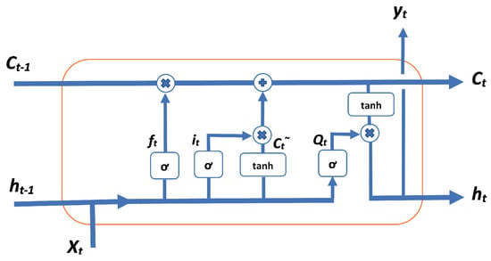
Figure 1.
One Long Short-Term Memory (LSTM) block structure.
- is the activation vector of the forget gate,
- is the sigmoid function,
- W is weight matrices to be learned during training,
- is input vector to the LSTM unit,
- b is bias vector parameters to be learned during training,
- is activation vector of the input gate,
- is cell state vector,
- is activation vector of the output gate, and
- is output vector of the LSTM unit.
4. Data Preparation and Results
In this research, we used kidney cancer RNA-sequence data represented by the miRNA expression that is publicly available on The Cancer Genome Atlas (TCGA) database website. For kidney cancer, three TCGA and two TARGET projects defined the most relevant kidney cancer types as High-Risk Wilms Tumor, Kidney Renal Clear Cell Carcinoma, Kidney Renal Papillary Cell Carcinoma, Kidney Chromophobe, Rhabdoid Tumor and Clear Cell Sarcoma of the Kidney. Figure 2 shows the sub-types project name and the percentage of cases for each project that are available in the TCGA data repository. From Table 1. one can see that the miRNA data is associated with the kidney cancer sub-types. The column “No. of Files” represents the available miRNA files for the cases. Please note that for some cases, more than one file is present, which is because of multiple readings for these cases during the diagnosis time.
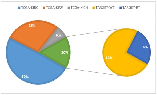
Figure 2.
Kidney diseases projects available in the The Cancer Genome Atlas (TCGA) data repository.

Table 1.
Table Type Styles.
4.1. Data Preparation and Categorization
We have considered all kidney cancer cases in which miRNA information was provided. These cases represent the samples taken from patients who had kidney cancer which belonged to one of five different cancer sub-types. Some individual cases had more than one miRNA sequence data file, which were represented by both isoform expression quantification and miRNA expression quantification. In our study, we only considered the miRNA expression qualification data because it tabulated in a balanced way, i.e., all cases had the same number of miRNAs.
Figure 3 shows the schematic diagram for the data preparation procedure. The data from the TCGA server was downloaded, and then it was categorized using a MATLAB program. First, the information related to each case was matched with its corresponding miRNA quantification files using the file ID. The information of miRNA read per million for each miRNA was considered in our experiment. The miRNA files were then matched with those in clinical data, stored in javascript file, using the case ID. This clinical data provides the record of cancer sub-types and other patient clinical information such as age, sex, and demographics. The above procedure of preparing the cancer data facilitated automatic classification of kidney cancer sub-types based on the miRNA quantification expression information of the patients.

Figure 3.
Data preparation for kidney cancer subtype classification.
With the procedure given above, we obtained all of the miRNAs provided. However, we noticed that many miRNAs had null readings. By removing those fields, we ended up with a total of 1627 out of 1881 miRNA and 1221 cases, which were grouped into the five subtypes as mentioned in Figure 2 and Table 1.
4.2. Results and Discussions
After we categorized and prepared the data from the TCGA repository, we checked the data points and found out that the data variation was too large, therefore it needed to be normalized. For this purpose, a logarithmic kernel was first applied to reduce the variance of the data points, then a normalization procedure was devised to ensure that the data points obeyed zero mean and unit variance.
Once the data was ready, we fed the labeled data files to a feature selection algorithm. We hypothesized that if all the miRNAs were used for cancer subtype classification, it would produce the best possible outcomes. We tested this hypothesis with an experiment as follows. First, we used all the data points without dimension reduction, and then used the NCA algorithm without regularization for five kidney cancer subtype classification. Indeed, we found out that the former in general produced better results. However, one would not know which miRNAs are more important for the classification if all the miRNAs are used. It is therefore important to select the miRNAs that have high discriminative capability.
To find the most discriminative miRNAs, the value of in the NCA algorithm needs to be tuned. For this, a five-fold cross-validation test was performed. For each fold, randomly selected of the data is used as a training set, and the remaining of the data as a test set. To produce reproducible results, the procedure needs to be repeated 10 times. Figure 4 shows the the average loss values of the five-fold validation verses values.
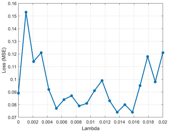
Figure 4.
The average loss values versus lambda () values.
Using the tuned value, NCA is applied to find the maximum weighted features, i.e., the most effective miRNAs that have the greatest discriminative power among the kidney cancer subtypes. Figure 5 shows the selected miRNAs according to NCA features weight value. Having a higher feature weight corresponds with better discriminative power for subtype classification. Table 2 shows the values of the selected Feature weight with corresponding miRNA name and index, where the indices of the miRNAs as appeared in the kidney cancer Quantified RNA sequence files in TCGA.
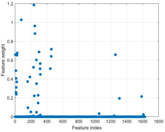
Figure 5.
The selected features/miRNAs according to NCA feature weights. A higher weight value indicates better discrimination power. A threshold of 0.02 was applied to reduce the number of miRNAs to 35.

Table 2.
Selected miRNA names and index with corresponding feature weights.
In the classification phase, we adopted the LSTM network algorithm with two LSTM layers. The first hidden layer had 500 neurons and the second one had 250 neurons. The hardware platform was NVIDIA TITAN X GPU. Ten runs of randomized five-fold validation was adopted for data analysis. The procedure followed largely the Data Analysis Protocol (DAP), which was defined by the US-FDA MAQC-II initiative [31]. Both the selected miRNA subset and the complete miRNA dataset were trained using the LSTM network. In each five-fold validation, a procedure of randomizing all the data points was performed for both the training and testing sets, whose average values were used to compute the total confusion matrices, which are given in Figure 6 and Figure 7, where indices of the classes are as follows: class 1 = WT, class 2 = KICH, class 3 KIRC, class 4 = KIRP, and class 5 = RT.

Figure 6.
Classification results using all of the 1627 miRNAs as features.
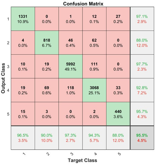
Figure 7.
Classification results using the 35 selected miRNAs as features.
It can be observed in this experimental study that using only the 35 selected miRNAs as features performs competitively with using all the available miRNAs.
One issue with the results presented in Figure 6 and Figure 7 was that the dataset was not balanced. For instance, the number of the Kidney Renal Clear Cell Carcinoma cases (class 1) is far greater than that of the Rhabdoid Tumor cases (class 5); refer to Table 1. Therefore, the training set for each class needs to be balanced to obtain unbiased classification results. For this purpose, a data augmentation procedure, given in [32], was applied. Small, random Gaussian noise with zero Mean and 0.02 variance was added to the data points of those classes with fewer cases, resulting in a balanced dataset. It is essential that the test set samples are removed before data augmentation. One-fifth of each subtype dataset was randomly selected and reserved for this purpose in a five-fold validation process, and then the training set was augmented to have 475 training samples for each subtype set. This process was repeated 10 times to archive the 10 × 5-Cross Validation, and the results were averaged to construct the confusion matrices as shown in Figure 8 and Figure 9.

Figure 8.
Classification accuracy of balanced training of 1627 miRNAs.
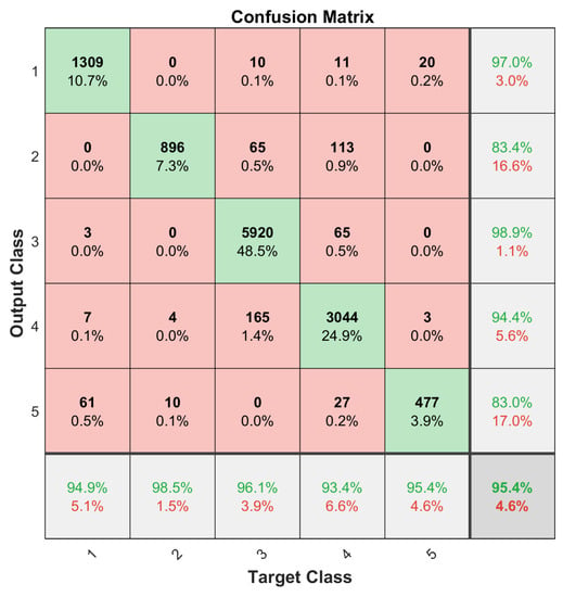
Figure 9.
Classification accuracy of balanced training of 35 selected miRNAs by NCA.
To further assess the classification performance, Matthews Correlation Coefficient (MCC) [6] was adopted. The MCC is given by the following equation:
In order to compute MCC, the true positive (), true negative (), false positive (), and false negative () were extracted as shown in Table 3 and Table 4.

Table 3.
The extracted true positive, true negative, false positive, and false negative from the unbalanced dataset.

Table 4.
The extracted true positive, true negative, false positive, and false negative from the balanced dataset.
The multiclass generalization of the MCC, refer to [33], for the cells of the confusion matrix C is given in Table 5. The proposed method was able to achieve an average classification accuracy of 97.2% and an MCC of 0.949 if all the available miRNAs were used and if the dataset was balanced. If not balanced, the accuracy is reduced to 92.9% and the MCC value to 0.887. With the 35 selected miRNA, the accuracy was 95.4% for both and the MCC values were 0.92 and 0.924, respectively (Figure 6, Figure 7, Figure 8 and Figure 9 and Table 5). It is clear that using the selected set of miRNAs, one can achieve a more consistent performance, in terms of both classification accuracy and MCC [34]. The result also shows that the selected 35 miRNAs performed better without data augmentation, compared to those obtained by using all of the available miRNAs (Table 5).

Table 5.
Classification performance in terms of Matthews Correlation Coefficients.
5. Conclusions
In this paper, we reported a machine learning approach for the classification of five subtypes of kidney cancer. In this approach, the NCA procedure was applied to select the most discriminative miRNAs as features and the LSTM neural network was designed to classify the given patient data files into five subtypes of kidney cancer. The Data Analysis Protocol was largely adopted to control the experiments and the Matthews Correlation Coefficient, together with accuracy, to assess the classification performance.
We demonstrated that with all of the available miRNAs, the proposed method produced an accuracy of 97.2% and an MCC value of 0.924 using an augmented dataset. We further demonstrated that with a subset of 35 miRNAs, the method achieved a more consistent classification performance for both balanced and unbalanced datasets in terms of both accuracy and MCC values. This demonstrates the importance of most discriminate miRNAs in cancer subtype diagnosis and classification.
We hope that the proposed method can be a step forward in the direction of early diagnosis of kidney cancers, which in turn will allow physicians to have better options in treating kidney cancer patients. We also hope that the identified miRNAs in this study can be used as biomarker candidates for kidney cancer subtype classification, though we understand that the effectiveness of these selected miRNAs must be validated by wet-lab experiments and further clinic studies.
Author Contributions
A.M.A. and H.Z. conceived and designed the experiments; A.M.A. and A.I. performed the experiments; M.H. and A.W. did literature survey; A.M.A. and A.I. analyzed the data; A.M.A., H.Z., O.R. and M.H. wrote the paper.
Funding
This research was partially funded by US National Science Foundation grant number 1624497. Ali Ibrahim was partially funded by a grant from GtechProcure.
Acknowledgments
We would like to thank National Cancer Institute and National Human Genome Research Institute for providing us with the TCGA data portal and Nvidia for the hardware platform. This work was partially supported by an NSF Phase II I/UCRC grant. Furthermore, we would like to thank GTech Procure and HCED for their sponsorship. The authors would also like to thank anonymous reviewers for suggesting the Data Analysis Protocol of US-FDA to evaluate the experimental results.
Conflicts of Interest
The authors declare no conflict of interest.
References
- Verbiest, A.; Couchy, G.; Job, S.; Caruana, L.; Lerut, E.; Oyen, R.; de Reyniès, A.; Tosco, L.; Joniau, S.; Van Poppel, H.; et al. Molecular subtypes of clear-cell renal cell carcinoma are prognostic for outcome after complete metastasectomy. Eur. Urol. 2018, 74, 474–480. [Google Scholar] [CrossRef] [PubMed]
- NCI. The NHGRI. The Cancer Genome Atlas Homepage. Available online: https://cancergenome.nih.gov/ (accessed on 28 April 2009).
- Yang, W.; Wang, K.; Zuo, W. Neighborhood Component Feature Selection for High-Dimensional Data. JCP 2012, 7, 161–168. [Google Scholar] [CrossRef]
- Hochreiter, S.; Schmidhuber, J. Long short-term memory. Neural Comput. 1997, 9, 1735–1780. [Google Scholar] [CrossRef] [PubMed]
- Ibrahim, A.K.; Zhuang, H.; Chérubin, L.M.; Schärer-Umpierre, M.T.; Erdol, N. Automatic classification of grouper species by their sounds using deep neural networks. J. Acoust. Soc. Am. 2018, 144, EL196–EL202. [Google Scholar] [CrossRef] [PubMed]
- Matthews, B.W. Comparison of the predicted and observed secondary structure of T4 phage lysozyme. Biochim. Biophys. Acta 1975, 405, 442–451. [Google Scholar] [CrossRef]
- Friedman, R.C.; Farh, K.K.H.; Burge, C.B.; Bartel, D.P. Most mammalian mRNAs are conserved targets of microRNAs. Genome Res. 2008, 19, 92–105. [Google Scholar] [CrossRef] [PubMed]
- Ambros, V. The functions of animal microRNAs. Nature 2004, 431, 350. [Google Scholar] [CrossRef] [PubMed]
- Jansson, M.D.; Lund, A.H. MicroRNA and cancer. Mol. Oncol. 2012, 6, 590–610. [Google Scholar] [CrossRef] [PubMed]
- Croce, C.M. Causes and consequences of microRNA dysregulation in cancer. Nat. Rev. Genet. 2009, 10, 704. [Google Scholar] [CrossRef] [PubMed]
- Lu, J.; Getz, G.; Miska, E.A.; Alvarez-Saavedra, E.; Lamb, J.; Peck, D.; Sweet-Cordero, A.; Ebert, B.L.; Mak, R.H.; Ferrando, A.A.; et al. MicroRNA expression profiles classify human cancers. Nature 2005, 435, 834. [Google Scholar] [CrossRef] [PubMed]
- Munker, R.; Calin, G.A. MicroRNA profiling in cancer. Clin. Sci. 2011, 121, 141–158. [Google Scholar] [CrossRef] [PubMed]
- Volinia, S.; Calin, G.A.; Liu, C.G.; Ambs, S.; Cimmino, A.; Petrocca, F.; Visone, R.; Iorio, M.; Roldo, C.; Ferracin, M.; et al. A microRNA expression signature of human solid tumors defines cancer gene targets. Proc. Natl. Acad. Sci. USA 2006, 103, 2257–2261. [Google Scholar] [CrossRef] [PubMed]
- Papadopoulos, E.I.; Petraki, C.; Gregorakis, A.; Fragoulis, E.G.; Scorilas, A. Clinical evaluation of microRNA-145 expression in renal cell carcinoma: A promising molecular marker for discriminating and staging the clear cell histological subtype. Biol. Chem. 2016, 397, 529–539. [Google Scholar] [CrossRef] [PubMed]
- White, N.M.; Bao, T.T.; Grigull, J.; Youssef, Y.M.; Girgis, A.; Diamandis, M.; Fatoohi, E.; Metias, M.; Honey, R.J.; Stewart, R.; et al. miRNA profiling for clear cell renal cell carcinoma: Biomarker discovery and identification of potential controls and consequences of miRNA dysregulation. J. Urol. 2011, 186, 1077–1083. [Google Scholar] [CrossRef] [PubMed]
- Juan, D.; Alexe, G.; Antes, T.; Liu, H.; Madabhushi, A.; Delisi, C.; Ganesan, S.; Bhanot, G.; Liou, L.S. Identification of a microRNA panel for clear-cell kidney cancer. Urology 2010, 75, 835–841. [Google Scholar] [CrossRef] [PubMed]
- Samaan, S.; Khella, H.W.; Girgis, A.; Scorilas, A.; Lianidou, E.; Gabril, M.; Krylov, S.N.; Jewett, M.; Bjarnason, G.A.; El-said, H.; et al. miR-210 is a prognostic marker in clear cell renal cell carcinoma. J. Mol. Diagn. 2015, 17, 136–144. [Google Scholar] [CrossRef] [PubMed]
- Zhang, W.; Ni, M.; Su, Y.; Wang, H.; Zhu, S.; Zhao, A.; Li, G. MicroRNAs in serum exosomes as potential biomarkers in clear-cell renal cell carcinoma. Eur. Urol. Focus 2016, 4, 412–419. [Google Scholar] [CrossRef] [PubMed]
- Vergho, D.; Kneitz, S.; Rosenwald, A.; Scherer, C.; Spahn, M.; Burger, M.; Riedmiller, H.; Kneitz, B. Combination of expression levels of miR-21 and miR-126 is associated with cancer-specific survival in clear-cell renal cell carcinoma. BMC Cancer 2014, 14, 25. [Google Scholar] [CrossRef] [PubMed]
- Zaman, M.S.; Shahryari, V.; Deng, G.; Thamminana, S.; Saini, S.; Majid, S.; Chang, I.; Hirata, H.; Ueno, K.; Yamamura, S.; et al. Correction: Up-Regulation of MicroRNA-21 Correlates with Lower Kidney Cancer Survival. PLoS ONE 2012, 7, e31060. [Google Scholar] [CrossRef]
- Wach, S.; Nolte, E.; Theil, A.; Stöhr, C.; Rau, T.; Hartmann, A.; Ekici, A.; Keck, B.; Taubert, H.; Wullich, B. MicroRNA profiles classify papillary renal cell carcinoma subtypes. Br. J. Cancer 2013, 109, 714. [Google Scholar] [CrossRef] [PubMed]
- White, N.; Khella, H.; Grigull, J.; Adzovic, S.; Youssef, Y.; Honey, R.; Stewart, R.; Pace, K.; Bjarnason, G.; Jewett, M.; et al. miRNA profiling in metastatic renal cell carcinoma reveals a tumour-suppressor effect for miR-215. Br. J. Cancer 2011, 105, 1741. [Google Scholar] [CrossRef] [PubMed]
- Youssef, Y.M.; White, N.M.; Grigull, J.; Krizova, A.; Samy, C.; Mejia-Guerrero, S.; Evans, A.; Yousef, G.M. Accurate molecular classification of kidney cancer subtypes using microRNA signature. Eur. Urol. 2011, 59, 721–730. [Google Scholar] [CrossRef] [PubMed]
- Petillo, D.; Kort, E.J.; Anema, J.; Furge, K.A.; Yang, X.J.; Teh, B.T. MicroRNA profiling of human kidney cancer subtypes. Int. J. Oncol. 2009, 35, 109–114. [Google Scholar] [CrossRef] [PubMed]
- Wang, J.; Lee, A.; Huang, M.; Ibrahim, A.K.; Zhuang, H.; Muhamed Ali, A. Classification of White Blood Cells with PatternNet-fused Ensemble of Convolutional Neural Networks (PECNN). In Proceedings of the International Symposium on Signal Processing and Information Technology (ISSPIT), Louisville, KY, USA, 6–8 December 2018. [Google Scholar]
- Wang, J.; Ibrahim, A.K.; Zhuang, H.; Muhamed Ali, A.; Li, A. A Study on Automatic Detection of IDC Breast Cancer with Convolutional Neural Networks. In Proceedings of the 2018 International Conference on Computational Science and Computational Intelligence (CSCI’18), Las Vegas, NV, USA, 13–15 December 2018. [Google Scholar]
- Mobiny, A.; Moulik, S.; Gurcan, I.; Shah, T.; Van Nguyen, H. Lung Cancer Screening Using Adaptive Memory-Augmented Recurrent Networks. arXiv, 2017; arXiv:1710.05719. [Google Scholar]
- Ypsilantis, P.P.; Montana, G. Recurrent convolutional networks for pulmonary nodule detection in CT imaging. arXiv, 2016; arXiv:1609.09143. [Google Scholar]
- Bychkov, D.; Linder, N.; Turkki, R.; Nordling, S.; Kovanen, P.E.; Verrill, C.; Walliander, M.; Lundin, M.; Haglund, C.; Lundin, J. Deep learning based tissue analysis predicts outcome in colorectal cancer. Sci. Rep. 2018, 8, 3395. [Google Scholar] [CrossRef] [PubMed]
- Zheng, Y.; Liu, D.; Georgescu, B.; Xu, D.; Comaniciu, D. Deep Learning Based Automatic Segmentation of Pathological Kidney in CT: Local Versus Global Image Context. In Deep Learning and Convolutional Neural Networks for Medical Image Computing; Springer: Berlin, Germany, 2017; pp. 241–255. [Google Scholar]
- Maggio, V.; Chierici, M.; Jurman, G.; Furlanello, C. A multiobjective deep learning approach for predictive classification in Neuroblastoma. arXiv, 2017; arXiv:1711.08198. [Google Scholar]
- DeVries, T.; Taylor, G.W. Dataset augmentation in feature space. arXiv, 2017; arXiv:1702.05538. [Google Scholar]
- Gorodkin, J. Comparing two K-category assignments by a K-category correlation coefficient. Comput. Biol. Chem. 2004, 28, 367–374. [Google Scholar] [CrossRef] [PubMed]
- Boughorbel, S.; Jarray, F.; El-Anbari, M. Optimal classifier for imbalanced data using Matthews Correlation Coefficient metric. PLoS ONE 2017, 12, e0177678. [Google Scholar] [CrossRef] [PubMed]
© 2018 by the authors. Licensee MDPI, Basel, Switzerland. This article is an open access article distributed under the terms and conditions of the Creative Commons Attribution (CC BY) license (http://creativecommons.org/licenses/by/4.0/).