Sparse and Low-Rank Subspace Data Clustering with Manifold Regularization Learned by Local Linear Embedding

Abstract

Data clustering is an important research topic in data mining and signal processing communications. In all the data clustering methods, the subspace spectral clustering methods based on self expression model, e.g., the Sparse Subspace Clustering (SSC) and the Low Rank Representation (LRR) methods, have attracted a lot of attention and shown good performance. The key step of SSC and LRR is to construct a proper affinity or similarity matrix of data for spectral clustering. Recently, Laplacian graph constraint was introduced into the basic SSC and LRR and obtained considerable improvement. However, the current graph construction methods do not well exploit and reveal the non-linear properties of the clustering data, which is common for high dimensional data. In this paper, we introduce the classic manifold learning method, the Local Linear Embedding (LLE), to learn the non-linear structure underlying the data and use the learned local geometry of manifold as a regularization for SSC and LRR, which results the proposed LLE-SSC and LLE-LRR clustering methods. Additionally, to solve the complex optimization problem involved in the proposed models, an efficient algorithm is also proposed. We test the proposed data clustering methods on several types of public databases. The experimental results show that our methods outperform typical subspace clustering methods with Laplacian graph constraint.

1. Introduction

Data clustering or segmentation is an active research topic in data mining, signal processing and unsupervised learning [1,2]. In practice, many data are generated from a space which has intrinsic subspace structure, i.e., the space is composed of union of multiple subspaces. In this case, it is necessary to exploit and reveal the subspace structure, and so different subspace clustering methods were proposed in recent years [3,4]. In all of the subspace clustering methods, the spectral clustering methods based on the affinity matrix of data are considered to have good prospects. The typical methods are the Sparse Subspace Clustering (SSC) [5] and the Low Rank Representation (LRR) methods [6]. The key problems of the subspace spectral clustering are how to find the proper data representation and how to construct the affinity or similarity matrix of the data for spectral clustering. In SSC and LRR methods, the original data are firstly represented by the self expression model with sparse or low-rank constraints. Then the affinity matrix is constructed from the representation coefficients. Using the affinity matrix as input, the final clustering results can be obtained by common spectral clustering algorithms, such as K-means or NCut methods.

It is critical for the spectral subspace clustering methods to construct a proper affinity matrix; one should exploit the data intrinsic properties to form necessary regularization for the data representation model. Based on the assumption that the data sample could only be represented by the samples coming from the same subspace it belongs to, SSC adds sparse constraint onto the representation coefficients matrix by $l_1$ norm [7]. However, the sparse constraint in SSC is an individual constraint for each datum representation. There is no consideration of correlation among the data. For this purpose, LRR adds the holistic constraint of low rank onto the representation coefficients matrix by using nuclear norm ${\parallel ·\parallel }_{*}$, which has been proved to be more helpful to reveal the subspace structure of the data drawn from the true multiple subspaces combined space [6].

Although SSC and LRR clustering methods have shown good clustering performance, the data representation is just formulated by sparse or low rank constraints. The other properties of the data or its representation are not well exploited. For example, in the real world, many high dimensional data are often considered to reside in low-dimensional manifolds space and to have non-linear geometrical structure. The sparse manifold clustering and embedding method [8] showed that introducing the local manifold structure can enhance the clustering performance for the data with non-linear property. However, the basic LRR and SSC methods do not take into account this manifold structure for high dimensional data. As a result, some non-linear metric related properties within data may be corrupted in the procedure of clustering. Observing that, numerous researchers have revised the basic SSC and LRR methods to model the data intrinsic properties by introducing extra constraint or regularization. Zheng et al. [9] proposed a graph regularized sparse coding method to obtain data sparse representations with the constraint of local manifold structure. Gao et al. [10] proposed two types of Laplacian regularizer by incorporating a similarity preserving term into the sparse representation model. Cai et al. [11] developed a graph-based approach for non-negative matrix factorization in order to represent the naive geometric structure in data. He et al. [12] proposed a Laplacian regularized Gaussian mixture model for data clustering by exploiting the probability distribution of the intrinsic manifold structure of data. Incorporating manifold regularization, Zhang et al. [13] proposed a novel low rank matrix factorization model for data representation. Hu et al. [14] proposed a SMooth Representation (SMR) model to enforce grouping effect in the data representation model. Liu et al. [15] proposed a Laplacian regularized LRR (LapLRR) to enhance low-rank subspace clustering by utilizing manifold property of data. Peng at el. [16] improved the low-rank representation via sparse manifold adaption for semi-supervised learning. Yin et al. [17] proposed a Non-negative Sparse Laplacian regularized LRR model (NSLLRR) to improve the performance of LRR. Recently, Wang et al. [18] proposed a LRR model on Grassmann manifold with Laplacian graph constraint. Yin et al. [19] proposed an adaptive way to construct the affinity matrix for eliminating the interference of noise in data. Except for the above Laplacian graph constraints, other constraints like the block-diagonal form of the affinity matrix [20,21,22] and the covariance of the data [23] are also exploited to improve subspace clustering performance.

In spite of obtaining improvement by utilizing the non-linear property hiding in the high dimensional data, most of the current methods justly represent this non-linear property by the Laplacian graph constructed directly from the similarity of the raw data under Euclidean distance, which is hard to fulfill modeling the intrinsic manifold structure. Additionally, these methods are easily biased by the noise and outliers existing in the raw data. Facing these problems, we think that the manifold learning methods, such as Local Linear Embedding (LLE) [24], Isomap [25] and Laplacian Eigenmaps (LE) [26], etc. give a possible solution, as they adopt a data-driven manner to learn and represent the non-linear structure of data and show robustness to noise or outliers. So we try to integrate manifold learning methods and the subspace clustering methods, and construct a subspace clustering method for high dimensional data based on manifold learning. Here, we adopt the classic LLE manifold learning method to learn the non-linear structure in the data and embed it into SSC and LRR subspace clustering procedure, thus we propose two new subspace clustering methods, namely LLE-SSC and LLE-LRR. The main contributions of this paper are listed as follows:

• A new framework of clustering is constructed by integrating the manifold learning methods with subspace clustering methods.
• Instead of building the Laplacian graph from the raw data, the manifold learning method, LLE, is adopted to reveal the non-linear property of the data for clustering, and this strategy is considered superior in dealing with noise and outliers.
• To solve the complicated optimization problem involved in the proposed LLE-SSC and LLE-LRR models, an efficient algorithm is determined as the solution.

The rest of the paper is organized as follows. In Section 2, we summarize the SSC and LRR subspace clustering methods and review the related works of our model. In Section 3, our proposed models, LLE-SSC and LLE-LRR, are described in detail and their solutions are given. In Section 4, the performance of the proposed method is evaluated on several public datasets. Finally, conclusions and future work are provided in Section 5.

2. Related Works

Our work is based on the classic SSC and LRR subspace methods, which make impressive progression and have state of the art clustering performance. In the following, we give a review of these two methods and discuss some related subspace clustering works.

The SSC and LRR subspace clustering methods are typical spectral clustering methods, which generally have two steps to implement clustering. First, the raw data are represented over a dictionary for obtaining the data representation coefficients and constructing the affinity matrix; Second, based on the affinity matrix, the clustering is implemented by using common spectral clustering methods, e.g., K-mean or NCut. As the dictionary training procedure usually has a high cost of computation for large datasets, an alternative scheme is to use the data itself as the dictionary, known as the self-expression property of data [5]. The first step in SSC and LRR is the core step as the affinity matrix has significant influence for the clustering result. So, many works focus on constructing an optimal affinity matrix by exploiting different constraints or regularizations. In SSC and LRR methods, the sparse and low rank constraints are added for the data representation matrix, respectively.

For convenience, we denote the data for clustering by $\mathbf{X}=[{\mathbf{x}}_1,\dots ,{\mathbf{x}}_n]$, which are assumed being generated from k subspaces, i.e., $\mathbf{X}={\bigcup }_{j=1}^k{\mathbf{X}}_j$ s.t. ${\bigcap }_{j=1}^k{\mathbf{X}}_j=\varphi$ and $\forall {\mathbf{x}}_i\in \mathbf{X}$, $\exists {\mathbf{X}}_{j^{*}}$, ${\mathbf{x}}_i\in {\mathbf{X}}_{j^{*}}$. The objective of subspace clustering is to find the proper subspace for each datum. For this purpose, SSC implements clustering by representing the data as the sparse coefficients. The original SSC model is usually formulated as follows [5]:

$$\underset{\mathbf{Z}}{min}{\parallel \mathbf{X}-\mathbf{X}\mathbf{Z}\parallel }_F^2+\lambda {\parallel \mathbf{Z}\parallel }_1,\mathrm{s}.\mathrm{t}.diag\left(\mathbf{Z}\right)=0,$$

(1)

where $\mathbf{Z}$ is the sparse representation coefficient matrix and $\lambda$ is the weight to balance the data self representation error and the sparse representation term.

In SSC, the sparse constraint is just applied for the coefficient of each datum. However, the correlation among the whole dataset or its sparse representation coefficients are not described. Based on this observation, to further reveal the holistic sparsity of the data, LRR proposed using low rank constraint for the coefficient matrix. Additionally, to solve the NP-hard optimization problem with low rank constraint, the nuclear norm ${\parallel ·\parallel }_{*}$ is generally used to replace the low rank constraint. Thus the LRR model can be formulated as the following optimization model [6]:

$$\underset{\mathbf{Z}}{min}{\parallel \mathbf{X}-\mathbf{X}\mathbf{Z}\parallel }_{2,1}+\lambda {\parallel \mathbf{Z}\parallel }_{*},$$

(2)

where ${\parallel ·\parallel }_{2,1}$ norm is used to obtain robustness for noises and outliers.

The above SSC and LRR models only use sparse and low rank constraint to the data coefficients, while the other data intrinsic property, such as the non-linear structure of high dimensional data, is not considered. To reveal the non-linear property of high dimensional data, some researchers proposed to use the Laplacian graph constraint to model the local manifold structure of the data. The SMR method [14] enforces the grouping effect on the data representation matrix by using Laplacian graph constraint as follows:

$$\begin{array}{cc}\hfill \underset{\mathbf{Z}}{min}& {\parallel \mathbf{X}-\mathbf{X}\mathbf{Z}\parallel }_F^2+\lambda tr\left(\mathbf{Z}{\mathbf{L}}_{\mathbf{W}}{\mathbf{Z}}^T\right),\hfill \end{array}$$

(3)

where $\mathbf{Z}$ is the data self representation, and ${\mathbf{L}}_{\mathbf{W}}$ is the Laplacian graph matrix generally constructed from the local neighbours of each data sample. For example, from the local neighbourhood with K nearest neighbours of each data sample, a weight matrix $\mathbf{W}\in {\mathbb{R}}^{n\times n}$ can be constructed with the element ${\mathbf{W}}_{ij}$ defined as follows:

$${\mathbf{W}}_{ij}=\left\{\begin{array}{cc}1\hfill & \mathrm{if}{\mathbf{x}}_i\in N_K\left({\mathbf{x}}_j\right)or{\mathbf{x}}_j\in N_K\left({\mathbf{x}}_i\right);\hfill \\ 0\hfill & \mathrm{otherwise},\hfill \end{array}\right.$$

(4)

where $N_K\left({\mathbf{x}}_i\right)$ denotes the set of K nearest neighbors of ${\mathbf{x}}_i$. From the weight matrix $\mathbf{W}$, it is easy to get its Laplacian matrix ${\mathbf{L}}_{\mathbf{W}}$ with the following element:

$${\mathbf{L}}_{\mathbf{W}}(i,j)=\left\{\begin{array}{cc}-\mathbf{W}(i,j)\hfill & \mathrm{if}i\ne j;\hfill \\ \sum _{l\ne i}\mathbf{W}(i,l)\hfill & \mathrm{otherwise}.\hfill \end{array}\right.$$

(5)

The Laplacian matrix is looked at as a graph which represents the pairwise relation of the data. Intuitively, if two data points ${\mathbf{x}}_i$ and ${\mathbf{x}}_j$ are close in the intrinsic geometry of raw data, their data representations should preserve this property. So it is natural to combine the sparse in (1) or low rank constraint in (2) with the Laplacian graph constraint in (3) to obtain new clustering models. Thus, the LapLRR method [15] presented a manifold regularization for LRR characterized by adopting the Laplacian graph constraint as follows:

$$\begin{array}{c}\underset{\mathbf{Z}}{min}{\parallel \mathbf{X}-\mathbf{X}\mathbf{Z}\parallel }_F^2+{\lambda }_1{\parallel \mathbf{Z}\parallel }_{*}+\frac{{\lambda }_2}{2}tr\left(\mathbf{Z}{\mathbf{L}}_{\mathbf{W}}{\mathbf{Z}}^T\right)\mathrm{s}.\mathrm{t}.\mathbf{Z}\ge \mathbf{0},\hfill \end{array}$$

(6)

where $\mathbf{Z}\ge \mathbf{0}$ demands the elements of $\mathbf{Z}$ being nonnegative.

Considered that there usually exist noise and outliers in the raw data, the NSLLRR method [17] adopted sparse constraints both for the data reconstruction error and the data representation. Additionally, the method exploits the Laplacian matrix construction methods in different cases, which results a hyper Laplacian matrix even when the data sampling is insufficient. The NSLLRR model is shown as follows:

$$\underset{\mathbf{Z}}{min}{\parallel \mathbf{X}-\mathbf{XZ}\parallel }_1+{\gamma \parallel \mathbf{Z}\parallel }_{*}+\lambda {\parallel \mathbf{Z}\parallel }_1+\beta tr\left({\mathbf{ZL}}^h{\mathbf{Z}}^T\right),$$

(7)

where ${\mathbf{L}}^h$ is the hyper Laplacian matrix and $\lambda$, $\beta$ and $\gamma$ are penalty parameters for balancing the regularization terms.

In the above methods, the Laplacian graph constraint is generally constructed from the raw data samples under certain metric, which is easily interfered by the outliers or noise exiting in the original dataset. In this paper, we adopt a new strategy by using the manifold learning method to learn the underlining non-linear structure of the data and use the learned relation of the data to regularize the sparse and low rank representations. The manifold learning methods have been proved successful in representation of high dimensional data and robust to noise [24,25], thus it is considered more suitable to reveal the non-linear property of high dimensional data for clustering, and expected to obtain better clustering performance. In the following section, we will give the proposed methods in detail.

3. SSC and LRR Clustering with LLE Regularization

In this section, we first construct our LRR and SSC models with LLE regularization, i.e., LLE-SSC and LLE-LRR, then we give the models solution in detail.

3.1. The Proposed LLE-SSC and LLE-LRR Models

LLE is a classic manifold learning method for dimension reduction, which can discover non-linear structure in high dimensional data by exploiting the data local geometry by linear reconstruction. Additionally, LLE maps its input data into a single global coordinate system of lower dimensionality and does not involve local minima by generating highly non-linear embedding operation. For the given dataset $\mathbf{X}$, LLE is to find the optimal weight matrix $\mathbf{W}$ to minimize the following sum error of the data samples which are linearly represented by their neighbours:

$$\begin{array}{c}\underset{{\mathbf{W}}_{ij}}{min}\sum _{i=1}^n\parallel {\mathbf{x}}_i-\sum _{{\mathbf{x}}_j\in N\left({\mathbf{x}}_i\right)}{\mathbf{W}}_{ij}{\mathbf{x}}_j{\parallel }_2\mathrm{s}.\mathrm{t}.\sum _{{\mathbf{x}}_j\in N\left({\mathbf{x}}_i\right)}{\mathbf{W}}_{ij}=1,\hfill \end{array}$$

(8)

where $N\left({\mathbf{x}}_i\right)$ is the neighbourhood of ${\mathbf{x}}_i$, and ${\mathbf{W}}_{ij}=0$ if ${\mathbf{x}}_j\notin N\left({\mathbf{x}}_i\right)$. For convenience, the above objective function can be formulated as matrix form as follows:

$$\sum _{i=1}^n\parallel {\mathbf{x}}_i-\sum _{{\mathbf{x}}_j\in N\left({\mathbf{x}}_i\right)}{\mathbf{W}}_{ij}{\mathbf{x}}_j{\parallel }_2=tr\left(\mathbf{X}{(\mathbf{I}-\mathbf{W})}^T(\mathbf{I}-\mathbf{W}){\mathbf{X}}^T\right).$$

(9)

To this minimization problem, there exist several efficient solutions, such as the method in [24]. Once obtaining the solution, denoted by ${\mathbf{W}}^{*}$, which is regarded as the matrix encoding the manifold structure of the data, we can use ${\mathbf{W}}^{*}$ to construct the regularization for SSC and LRR. The argument is that the learned manifold property of the data $\mathbf{X}$ is also valid to its sparse or low rank representations $\mathbf{Z}$. In other words, if we replace $\mathbf{X}$ with $\mathbf{Z}$, the error in (8) will be still minimal as they share the same manifold structure.

If we assume

$${\mathbf{L}}_{\mathbf{M}}={(\mathbf{I}-{\mathbf{W}}^{*})}^T(\mathbf{I}-{\mathbf{W}}^{*}),$$

(10)

then we can obtain the LLE regularization as follows:

$$\begin{array}{c}\underset{\mathbf{Z}}{min}tr\left(\mathbf{Z}{\mathbf{L}}_{\mathbf{M}}{\mathbf{Z}}^T\right).\hfill \end{array}$$

(11)

Integrating the above regularization with SSC and LRR models, we naturally obtain our final LLE-SSC and LLE-LRR models as follows:

$$\begin{array}{c}\hfill \underset{\mathbf{Z}}{min}{\parallel \mathbf{Z}\parallel }_1+\frac{{\lambda }_1}{2}{\parallel \mathbf{X}-\mathbf{X}\mathbf{Z}\parallel }_F^2+{\lambda }_{2}tr\left(\mathbf{Z}{\mathbf{L}}_{\mathbf{M}}{\mathbf{Z}}^T\right),\end{array}$$

(12)

$$\begin{array}{c}\hfill \underset{\mathbf{Z}}{min}{\parallel \mathbf{Z}\parallel }_{*}+\frac{{\lambda }_1}{2}{\parallel \mathbf{X}-\mathbf{X}\mathbf{Z}\parallel }_F^2+{\lambda }_{2}tr\left(\mathbf{Z}{\mathbf{L}}_{\mathbf{M}}{\mathbf{Z}}^T\right).\end{array}$$

(13)

In practice, to avoid numerical instability, ${\mathbf{L}}_{\mathbf{M}}$ is generally added a disturbed value to enforce ${\mathbf{L}}_{\mathbf{M}}$ to be strictly positive definite, i.e., ${\mathbf{L}}_{\mathbf{M}}$ is replaced by ${\mathbf{L}}_{\mathbf{M}}={\mathbf{L}}_{\mathbf{M}}+\epsilon \mathbf{I}$ where $\mathbf{I}$ is the identity matrix and $0<\epsilon \ll 1$, the same as that in [14].

3.2. Solutions to LLE-SSC and LLE-LRR

For the problems in (12) and (13), we use the Alternating Direction Method of Multipliers (ADMM) [27] to find the solutions. To deal with the sparse item and the nuclear norm item of $\mathbf{Z}$ in (12) and (13), we separate the term of $\mathbf{Z}$ by introducing an auxiliary $\mathbf{S}$. Let $\mathbf{S}=\mathbf{Z}$, then the problems in (12) and (13) can be re-written as the following problems with the Augmented Lagrangian items for the introduced constraints,

$$\begin{array}{c}\hfill \underset{\mathbf{Z},\mathbf{S}}{min}{\parallel \mathbf{S}\parallel }_1+\frac{{\lambda }_1}{2}{\parallel \mathbf{X}-\mathbf{XZ}\parallel }_F^2+{\lambda }_{2}tr\left({\mathbf{ZL}}_{\mathbf{M}}{\mathbf{Z}}^T\right)+\langle \mathbf{G},\mathbf{Z}-\mathbf{S}\rangle +\frac{\gamma }{2}{\parallel \mathbf{Z}-\mathbf{S}\parallel }_F^2,\end{array}$$

(14)

$$\begin{array}{c}\hfill \underset{\mathbf{Z},\mathbf{S}}{min}{\parallel \mathbf{S}\parallel }_{*}+\frac{{\lambda }_1}{2}{\parallel \mathbf{X}-\mathbf{XZ}\parallel }_F^2+{\lambda }_{2}tr\left({\mathbf{ZL}}_{\mathbf{M}}{\mathbf{Z}}^T\right)+\langle \mathbf{G},\mathbf{Z}-\mathbf{S}\rangle +\frac{\gamma }{2}{\parallel \mathbf{Z}-\mathbf{S}\parallel }_F^2,\end{array}$$

(15)

where $\mathbf{G}$ is the Lagrangian multiplier and $\gamma$ is the increasing weight parameter enforcing $\mathbf{S}=\mathbf{Z}$. The problems in (14) and (15) can be solved by the following sub-problems with respect to $\mathbf{Z}$, $\mathbf{S}$ in an alternative manner by updating one when fixing the other.

(1) Fixing $\mathbf{S}$, solve for $\mathbf{Z}$   

When $\mathbf{S}$ is fixed, the objective functions in the problems in (14) and (15) will be transformed to the same objective function as follows:

$$\begin{array}{cc}\hfill f\left(\mathbf{Z}\right)=& \frac{{\lambda }_1}{2}{\parallel \mathbf{X}-\mathbf{XZ}\parallel }_F^2+{\lambda }_{2}tr\left({\mathbf{ZL}}_{\mathbf{M}}{\mathbf{Z}}^T\right)+\langle \mathbf{G},\mathbf{Z}-\mathbf{S}\rangle +\frac{\gamma }{2}{\parallel \mathbf{Z}-\mathbf{S}\parallel }_F^2.\hfill \end{array}$$

(16)

As $f\left(\mathbf{Z}\right)$ is a quadratic function with respect to $\mathbf{Z}$, we set the derivative of $f\left(\mathbf{Z}\right)$ to zero and have

$$\begin{array}{c}({\lambda }_1\mathbf{X}{\mathbf{X}}^T+\gamma \mathbf{I})\mathbf{Z}+{\lambda }_2{\mathbf{ZL}}_{\mathbf{M}}={\lambda }_1{\mathbf{X}}^T\mathbf{X}+\gamma \mathbf{S}-\mathbf{G}.\hfill \end{array}$$

(17)

Then vectorizing the matrix $\mathbf{Z}$, we can transform the above equation into the following linear equation and thus obtain the solution of $\mathbf{Z}$.

$$\begin{array}{c}\hfill \left(\mathbf{I}\otimes ({\lambda }_1{\mathbf{XX}}^T+\gamma \mathbf{I})+\lambda {\mathbf{L}}_{\mathbf{M}}\otimes \mathbf{I}\right)vec\left(\mathbf{Z}\right)=vec({\lambda }_1{\mathbf{X}}^T\mathbf{X}+\gamma \mathbf{S}-\mathbf{G}).\end{array}$$

(18)

(2) Fixing $\mathbf{Z}$, solve for $\mathbf{S}$   

When $\mathbf{Z}$ is fixed, the LLE-SSC and LLE-LRR optimization problems in (14) and (15) degenerate as the following problems:

$$\begin{array}{cc}\hfill \underset{\mathbf{S}}{min}& {\parallel \mathbf{S}\parallel }_1+\langle \mathbf{G},\mathbf{Z}-\mathbf{S}\rangle +\frac{\gamma }{2}{\parallel \mathbf{Z}-\mathbf{S}\parallel }_F^2,\hfill \end{array}$$

(19)

$$\begin{array}{cc}\hfill \underset{\mathbf{S}}{min}& {\parallel \mathbf{S}\parallel }_{*}+\langle \mathbf{G},\mathbf{Z}-\mathbf{S}\rangle +\frac{\gamma }{2}{\parallel \mathbf{Z}-\mathbf{S}\parallel }_F^2.\hfill \end{array}$$

(20)

Let $\mathbf{P}=\mathbf{Z}+\frac{\mathbf{G}}{\gamma }$, the above problems have the following equivalent forms:

$$\begin{array}{cc}\hfill \underset{\mathbf{S}}{min}& {\parallel \mathbf{S}\parallel }_1+\frac{\gamma }{2}{\parallel \mathbf{Z}-\mathbf{P}\parallel }_F^2,\hfill \end{array}$$

(21)

$$\begin{array}{cc}\hfill \underset{\mathbf{S}}{min}& {\parallel \mathbf{S}\parallel }_{*}+\frac{\gamma }{2}{\parallel \mathbf{Z}-\mathbf{P}\parallel }_F^2.\hfill \end{array}$$

(22)

For the problem in (21), it has a closed-form solution [28] given by

$$\begin{array}{c}\hfill \mathbf{S}=sign\left(\mathbf{P}\right)max\{|\mathbf{P}|-\frac{1}{\gamma },0\}.\end{array}$$

(23)

For the problem in (22), it also has a closed-form solution [29] given by

$$\mathbf{S}=\mathbf{U}Q\left[\mathsf{\Sigma }\right]{\mathbf{V}}^T,$$

(24)

where ${\mathbf{U}\mathsf{\Sigma }\mathbf{V}}^T$ is the singular value decomposition (SVD) of $\mathbf{P}$. $Q[·]$ is the soft-thresholding operator defined on the diagonal element ${\mathsf{\Sigma }}_{ii}$ of $\mathsf{\Sigma }$ as follows:

$$Q\left[{\mathsf{\Sigma }}_{ii}\right]=\left\{\begin{array}{cc}{\mathsf{\Sigma }}_{ii}-1,\hfill & \mathrm{if}{\mathsf{\Sigma }}_{ii}>1;\hfill \\ {\mathsf{\Sigma }}_{ii}+1,\hfill & \mathrm{if}{\mathsf{\Sigma }}_{ii}<-1;\hfill \\ 0,\hfill & \mathrm{otherwise}.\hfill \end{array}\right.$$

(25)

Once the above two steps are solved, the solutions to the proposed LLE-SSC and LLE-LRR models will be obtained. The complete algorithm for the data representation is summarized in Algorithm 1. It is denoted that the convergence of the ADMM method could not be guaranteed as being discussed in [30]. However, our following experiments show that the algorithm always converges. As to the complexity of Algorithm 1, the main computational cost of the algorithm is determined by the step 2, 3, 5 and 6. For the dataset $\mathbf{X}$ with n sample vectors in the dimension of D, the step 2 is to get the LLE weights ${\mathbf{W}}^{*}$ by solving (8) and its complexity is $\mathcal{O}(D{n}^2+(D+K)K^{2}n)$, where K is the maximal neighbours of the data samples. The calculation of ${\mathbf{L}}_{\mathbf{M}}$ in the step 3 has the complexity of $\mathcal{O}\left(n^2\right)$ according to (10). Step 5 is to solve the data representation matrix $\mathbf{Z}$ by the linear equation in (18), which has the complexity of $\mathcal{O}\left(T_0{\left(n^2\right)}^2\right)$, where $T_0$ is the maximal iterations of (18). The complexity of step 6 is different for LLE-SSC and LLE-LRR methods; the former has the complexity of $\mathcal{O}\left(n^2\right)$ and the latter has the complexity of $\mathcal{O}\left(r{n}^2\right)$ , where r is the estimated rank of the data representation matrix $\mathbf{S}$ or $\mathbf{Z}$. Inductively, we obtain the final complexity of Algorithm 1, i.e., $\mathcal{O}(T{T}_0{n}^4+(D+T+1)n^2+(D+K)K^{2}n)$ for LLE-SSC and $\mathcal{O}(T{T}_0{n}^4+(D+Tr+1)n^2+(D+K)K^{2}n)$ for LLE-LRR, respectively.

Algorithm 1 Solution to the data representation for LLE-SSC and LLE-LRR.

Input:  The dataset $\mathbf{X}$, maximal iteration number T, parameters ${\lambda }_1,{\lambda }_2,\gamma$. Output:  The data representation $\mathbf{Z}$. 1: Initialization: ${\mathbf{Z}}^0=0,{\mathbf{S}}^0=0,\mathbf{Z}=\mathbf{S},t=0,\mathbf{G}=\mathbf{I},\rho =1.3$. 2: Obtain ${\mathbf{W}}^{*}$ by solving (8); 3: Calculate ${\mathbf{L}}_{\mathbf{M}}$ by (10); 4: while$t<T$do 5:   Calculate ${\mathbf{Z}}^t$ by (18); 6:   If LLE-SSC, calculate ${\mathbf{S}}^t$ by (23); 7:   If LLE-LRR, calculate ${\mathbf{S}}^t$ by (24); 8:   Update $\mathbf{G}\leftarrow \mathbf{G}+\gamma ({\mathbf{Z}}^t-{\mathbf{S}}^t)$; 9:   Update $\gamma \leftarrow \rho \gamma$; 10:    Update $t\leftarrow t+1$; 11: end while

Based on the above LLE-SSC anf LLE-LRR data representation algorithm, we can finally obtain the subspace clustering algorithm as shown in Algorithm 2.

Algorithm 2 Subspace clustering based on LLE-SSC and LLE-LRR.

Input:  The data for clustering $\mathbf{X}$. Output:  The clustering results of $\mathbf{X}$. 1: Obtain the sparse representation $\mathbf{Z}$ of $\mathbf{X}$ by Algorithm 1; 2: Calculate the affinity matrix $\mathbf{W}=\left(\right|\mathbf{Z}|+|{\mathbf{Z}}^T\left|\right)/2$; 3: Calculate the Laplace matrix ${\mathbf{L}}_{\mathbf{W}}$ by (5); 4: Implement NCut$\left({\mathbf{L}}_{\mathbf{W}}\right)$ to get the final clustering result of $\mathbf{X}$.

4. Experiments

To evaluate the performance of the proposed methods, we implement clustering experiments on several public databases. Firstly, to test the proposed clustering methods in an ideal situation, we use a dataset with true subspace structure for clustering. Here, the synthetic dataset in [31] is adopted, which can be regarded as the baseline dataset for the subspace clustering methods. Then we test the proposed clustering methods on several real world datasets, including the Extended Yale B face dataset [32], the handwritten digit dataset of United States Postal Service (USPS) [33], the image dataset of COIL20 [34] and the motion track dataset, Hopkins155 [35], which are considered challenging for clustering as there is too much variety in these datasets.

The proposed methods, LLE-SSC and LLE-LRR, are compared with several related subspace methods, including the classic SSC and LRR methods, which are considered the baseline methods in subspace clustering methods. Additionally, the proposed methods are also compared with several variations of SSC and LRR, including SMR [14], LapLRR [15] and NSLLRR [17], which introduced other constraints for the data representation, like Laplacian graph, to improve the clustering performance. We summarize the metrics of the data representation error, the constraints for the data representation and the methods for constructing the Laplacian matrix in the related methods and our methods in

Table 1. The metrics of the data representation error, the constraints for the data representation and the methods for constructing the Laplacian matrix in the related methods and our methods.

Methods	Metrics of the Data Representation Error	Constraints for the Data Representation	Methods for Constructing the Laplacian Matrix
SSC [5]	${\parallel \mathbf{X}-\mathbf{XZ}\parallel }_F^2$	${\parallel \mathbf{Z}\parallel }_1$
LRR [6]	${\parallel \mathbf{X}-\mathbf{XZ}\parallel }_{2,1}$	${\parallel \mathbf{Z}\parallel }_{*}$
SMR[14]	${\parallel \mathbf{X}-\mathbf{XZ}\parallel }_F^2$	$tr\left({\mathbf{ZL}}_{\mathbf{W}}{\mathbf{Z}}^T\right)$	${\mathbf{L}}_{\mathbf{W}}$ is constructed from the relations of the samples and their neighbours.
LapLRR [15]	${\parallel \mathbf{X}-\mathbf{XZ}\parallel }_F^2$	${\parallel \mathbf{Z}\parallel }_{*}\mathrm{and}tr\left({\mathbf{ZL}}_{\mathbf{W}}{\mathbf{Z}}^T\right)$	${\mathbf{L}}_{\mathbf{W}}$ is constructed from the similarities of the samples and their neighbours.
NSLLRR [17]	${\parallel \mathbf{X}-\mathbf{XZ}\parallel }_1$	${\parallel \mathbf{Z}\parallel }_{*},{\parallel \mathbf{Z}\parallel }_1\mathrm{and}tr\left({\mathbf{ZL}}^h{\mathbf{Z}}^T\right)$	${\mathbf{L}}^h$ is constructed from multiple relationships between samples.
LLE-SSC	${\parallel \mathbf{X}-\mathbf{XZ}\parallel }_F^2$	${\parallel \mathbf{Z}\parallel }_1\mathrm{and}tr\left({\mathbf{ZL}}_{\mathbf{M}}{\mathbf{Z}}^T\right)$	${\mathbf{L}}^{\mathbf{M}}$ is learned by manifold learning method of LLE.
LLE-LRR	${\parallel \mathbf{X}-\mathbf{XZ}\parallel }_F^2$	${\parallel \mathbf{Z}\parallel }_{*}\mathrm{and}tr\left({\mathbf{ZL}}_{\mathbf{M}}{\mathbf{Z}}^T\right)$	${\mathbf{L}}^{\mathbf{M}}$ is learned by manifold learning method of LLE.

.

To evaluate the performance of these clustering methods, the Subspace Clustering Error (SCE) defined in [31] is adopted as the measurement with the following form:

$$\begin{array}{c}\hfill SCE=\frac{\mathrm{num}.\mathrm{misclssified}\mathrm{points}}{\mathrm{total}\mathrm{num}.\mathrm{of}\mathrm{points}},\end{array}$$

(26)

where “num.misclssified points” represents the number of misclassified samples, and “total num.of points” is the number of total samples.

There are two parameters ${\lambda }_1,{\lambda }_2$ which should be set in the proposed LLE-SSC and LLE-LRR methods. However, for the balancing parameters in optimization models, few effective methods are available to obtain the optimal value, as it is generally dependent on the specific datasets. So to get the proper values of these parameters, we adopt a tuning method based on a set of pre-experiments. Concretely, we change the values of these parameters in an estimated range, and for each selected value, we implement some clustering experiments. By comparing the clustering results with different values of these parameters, we can get the favorable values, though they may be not the global optimal values. In the following experiments, we will report the parameters setting for each dataset. The parameters of the compared methods are set as the same as the recommended setting in the original paper or tuned manually based on some pre-experiments similar to the above setting of ours.

4.1. Synthetic Experiment

In the synthetic experiment, we adopt the similar method in [31] to produce the data samples for clustering. Firstly, we randomly select five samples from the pure infrared hyper spectral mineral data and form a matrix ${\mathbf{A}}_i=[{\mathbf{a}}_1,\dots ,{\mathbf{a}}_5]\in {\mathbb{R}}^{321\times 5}$. Then we produce a random vector ${\mathbf{w}}_i\in {\mathbb{R}}^5$ by using a uniform distribution and obtain a vector by linear combination ${\mathbf{x}}_i={\mathbf{A}}_i{\mathbf{w}}_i$. Let the generation of ${\mathbf{w}}_i$ be repeated 10 times, we can obtain 10 data samples from the subspace $span\left({\mathbf{A}}_i\right)$, denoted by ${\mathbf{X}}_i=[{\mathbf{x}}_1,\dots ,{\mathbf{x}}_{10}]\in {\mathbb{R}}^{321\times 10}$. If we repeat the process of ${\mathbf{A}}_i$ five times, we finally get a dataset derived from the union of five subspaces, denoted by $\mathbf{X}=[{\mathbf{X}}_1,\dots ,{\mathbf{X}}_5]\in {\mathbb{R}}^{321\times 50}$, which will be used as the dataset for clustering. To further evaluate the robustness of the proposed methods, we add Gaussian noise onto $\mathbf{X}$ with three different magnitudes (10%, 20%, 30%) and so we produce three noisy datasets for clustering experiments. To get stable results, the experiments on different datasets are repeated 50 times with the reproduced $\mathbf{X}$. The minimum, maximum, median and mean clustering errors are recorded for complete evaluation. In the above experiments, the parameters ${\lambda }_1=20,{\lambda }_2=1$ for LLE-SSC and ${\lambda }_1=100,{\lambda }_2=1000$ for LLE-LRR.

The experimental results are shown in

Table 2. Clustering results on the synthetic hyper spectral mineral dataset with various magnitudes of Gaussian noise, lower is better. Numbers in brackets indicate how many times clustering was perfect, i.e., zero error. The best results are in bold font.

Gaussian Noise%		The Clustering Error
		SSC	LRR	NSLLRR	SMR	LapLRR	LLE-SSC	LLE-LRR
0	min	0.00% (50)	0.00% (49)	0.00% (44)	0.00% (50)	0.00% (50)	0.00% (46)	0.00% (50)
	max	0.00%	14.00%	24.00%	0.00%	0.00%	22.00%	0.00%
	med	0.00%	0.00%	0.00%	0.00%	0.00%	0.00%	0.00%
	mean	0.00%	14.28%	0.26%	0.00%	0.00%	0.36%	0.00%
10	min	0.00% (48)	0.00% (36)	0.00% (49)	0.00% (47)	0.00% (48)	0.00% (50)	0% (50)
	max	2.00%	30.00%	1.00%	2.00%	1.00%	0.00%	0.00%
	med	0.00%	0.00%	0.00%	0.00%	0.00%	0.00%	0.00%
	mean	0.08%	3.52%	0.20%	0.12%	0.04%	0.00%	0.00%
20	min	0.00% (10)	0.00% (10)	0.00% (13)	0.00% (15)	0.00% (15)	0.00% (32)	0.00% (27)
	max	42.00%	38.00%	28.00%	30.00%	26.00%	24.00%	34.00%
	med	8.00%	10.00%	4.00%	4.00%	4.00%	0.00%	0.00%
	mean	10.44%	12.80%	8.08%	8.80%	6.32%	4.20%	3.28%
30	min	4.00%	0.00% (2)	0.00% (1)	20.00%	8.00%	0.00% (5)	0.00% (6)
	max	56.00%	54.00%	44.00%	60.00%	70.00%	42.00%	38.00%
	med	36.00%	24.00%	24.00%	42.00%	42.00%	14.00%	15.00%
	mean	34.23%	25.24%	23.06%	43.84%	38.36	14.28%	16.08%

. In the noise free case, almost all clustering methods perform well; SSC, SMR, LapLRR and our model LLE-LRR have completely correct results. However, when the noise amplitude increases, the clustering performances of the compared methods decrease rapidly, while that of our methods drops slowly. It is shown that compared with the other methods, our LLE-SSC method has at least 10% improvements in metric of median and at least 8% improvements in metric of mean when the noise level is 30%, which highlights that our methods have good robustness to noise.

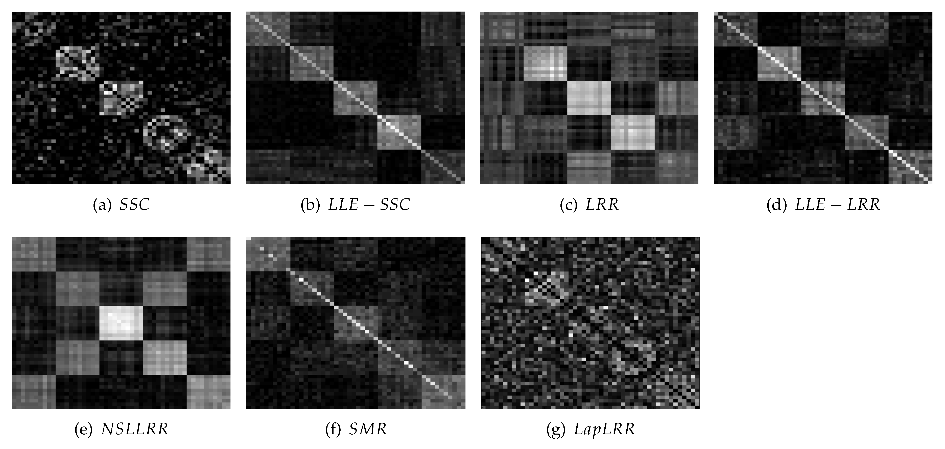
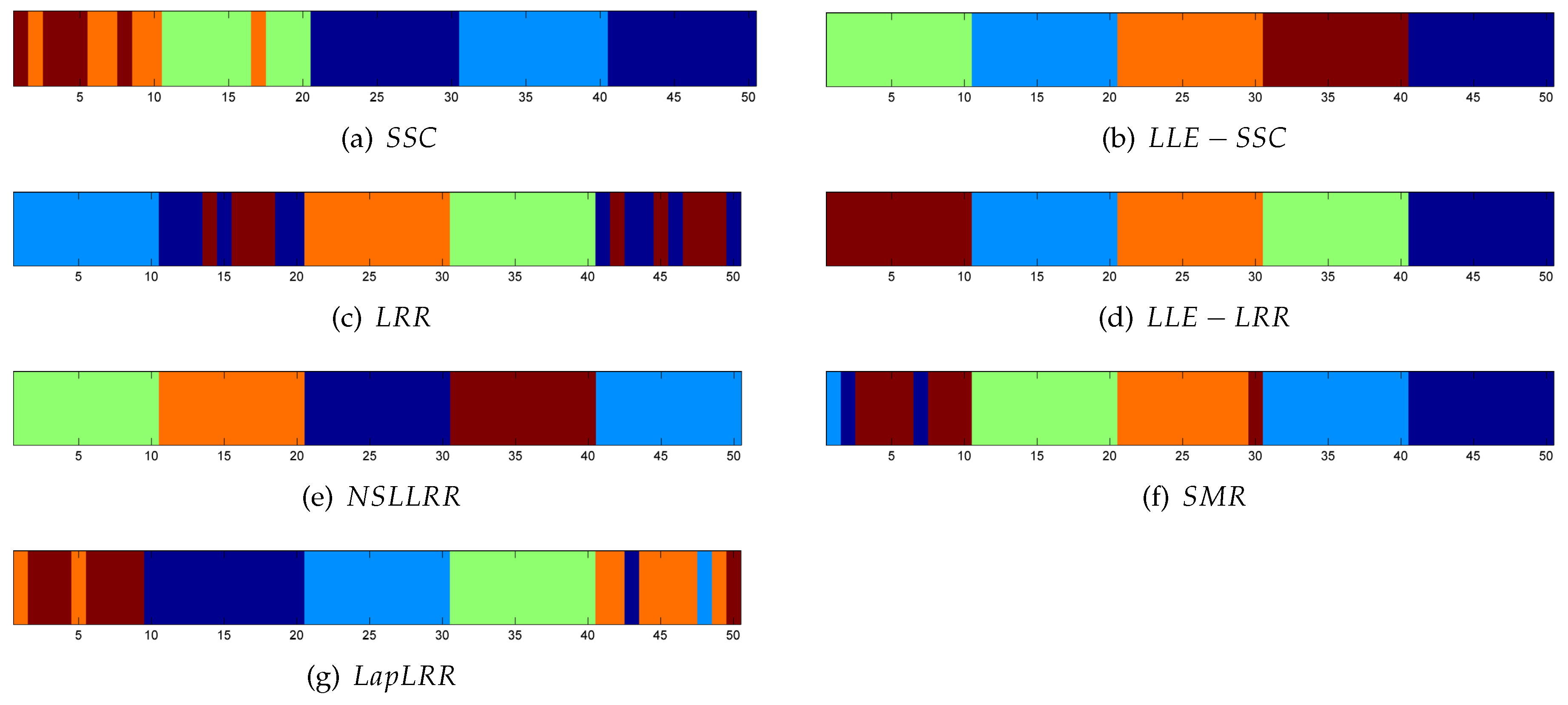
For the subspace clustering methods, the constructed affinity matrix is critical for clustering. The ideal affinity matrix will be a block diagonal form. Generally, the closer to the block diagonal form it is, the better the clustering results will be. Therefore, we provide a visual comparison of affinity matrices produced by different methods in case of adding 20% Gaussian noise, as shown in Figure 1. It is observed that our proposed methods, LLE-SSC and LLE-LRR, have affinity matrices closer to block diagonal shape than other methods. Additionally, we further show the clustering results by visualizing the samples of the same class with the same color, as shown in Figure 2. It is indicted that our methods, LLE-SSC, LLE-LRR and NSLLRR, have the best clustering results.

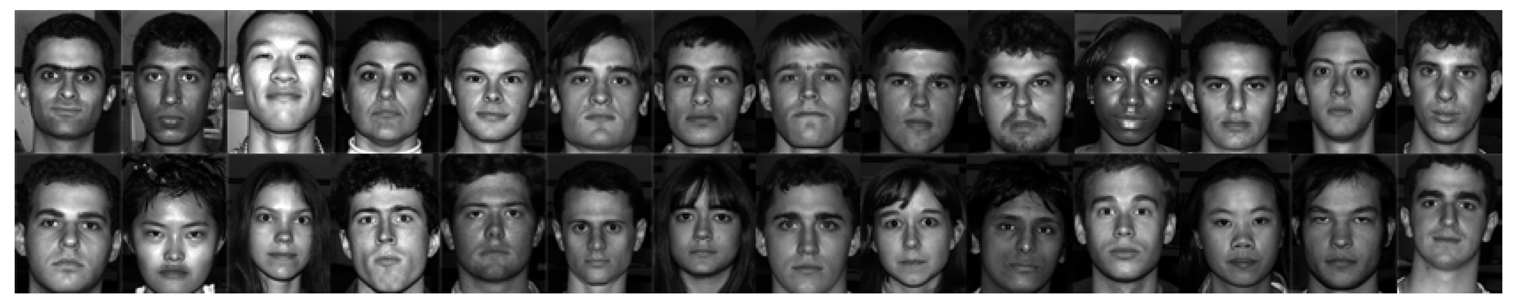
4.2. Face Clustering on Extended Yale B

To test the proposed LLE-SSC and LLE-LRR methods in more complicated scenarios, we perform clustering experiments on the wildly used face dataset, the Extended Yale B, which has face images of 38 persons captured under different illuminations with each person having 64 front face images. Some samples of the dataset are shown in Figure 3. For clustering application, this dataset is considered challenging as there exists too much varsity of illumination, expression and pose. Here, we randomly select $c=[2,3,5,8,10]$ people and each person chooses 32 face images for clustering. All images in our experiment are resized to 32 × 32 pixels. As a result, we obtain the initial sample vectors ${\mathbf{x}}_i\in {\mathbb{R}}^{1024}$. Then we reduce the dimension of these samples to (9 × c) by the Principal Component Analysis (PCA) method according to the similar data processing procedure in [20]. Based on the dimension reduced datasets, we implement clustering on the selected c classes. To get a stable result, we repeat the clustering experiments 30 times by re-selecting c classes of face images and use the mean clustering error as the final results. In the experiment, the parameters ${\lambda }_1=20,{\lambda }_2=1$ for LLE-SSC and ${\lambda }_1=3,{\lambda }_2=0.5\ast c$ for LLE-LRR.

The experimental results are reported in

Table 3. Clustering results on Extended Yale dataset B. The clustering errors for 2, 3, 5, 8, 10 classes and their mean error are shown here. The best results are in bold font.

Number of Classes	The Clustering Error (%)
	SSC	LRR	NSLLRR	SMR	LapLRR	SSC-LLE	LRR-LLE
2	7.74	6.87	3.22	3.49	4.09	2.00	1.23
3	10.83	9.81	5.42	6.16	5.13	2.91	1.80
5	23.81	18.01	17.01	9.05	10.84	3.31	2.78
8	32.47	33.81	31.94	21.23	20.92	3.53	3.18
10	34.73	36.15	34.33	28.36	25.52	3.68	3.55
mean	21.92	20.93	18.38	13.66	13.30	3.09	2.51

. It is observed that our methods significantly outperform the other methods in all cases. Both LLE-SSC and LLE-LRR have at least 10% improvements compared to the other methods in terms of the mean error of different number of classes. In addition, our methods have the advantage that the clustering performances decrease little when the number of classes increases. On the contrary, the clustering performances of other methods drop dramatically when the number of classes increases. This demonstrates that the proposed methods have the application potential for clustering large scale datasets.

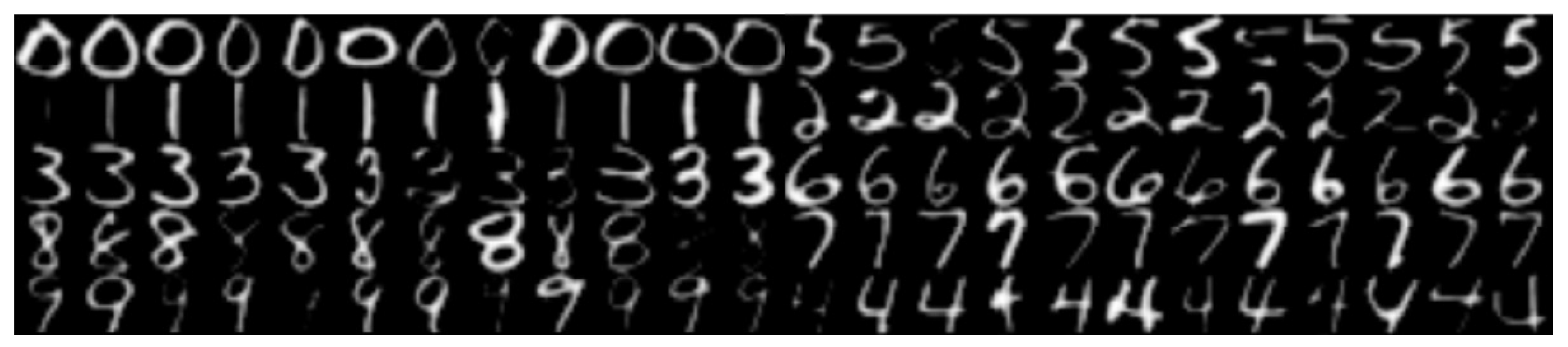
4.3. Handwritten Digit Clustering on USPS

In this experiment, we test the clustering performance of our methods on the handwritten digit dataset of USPS. In total, this dataset contains 9298 handwritten digit images of “0” through “9”, each of which is in the size of 16 × 16 pixels, with 256 gray levels per pixel. Some sample images are provided in Figure 4. We represent the digital images as 256-dimensional vectors and randomly select $c=[2,3,4,5,6,8,7,8,9,10]$ digits for clustering. For each selected digit, 48 images are randomly picked up. We repeat these clustering tests 30 times for each c digits and the mean clustering errors are computed. Here the parameters ${\lambda }_1=800,{\lambda }_2=$ 10,000 for LLE-SSC and ${\lambda }_1=1,{\lambda }_2=10$ for LLE-LRR.

Table 4. Clustering results on USPS dataset. The clustering errors for $2,3,4,5,6,7,8,9,10$ classes and their mean error are shown here. The best results are in bold font.

Number of Classes	The Clustering Error (%)
	SSC	LRR	NSLLRR	SMR	LapLRR	LLE-SSC	LLE-LRR
2	4.26	3.80	7.55	4.49	3.16	4.74	3.02
3	11.45	7.64	8.75	9.77	7.03	7.23	8.34
4	21.51	11.43	15.50	12.33	14.55	8.97	9.46
5	27.35	18.375	14.74	16.78	14.50	12.32	13.17
6	32.14	20.05	18.84	17.91	19.08	16.42	16.74
7	34.55	20.13	19.61	19.74	20.83	20.00	17.86
8	36.45	22.24	21.58	22.91	23.07	24.17	21.33
9	38.17	23.76	23.68	26.07	26.36	26.40	23.84
10	39.32	28.30	26.03	29.58	27.29	28.94	24.16
mean	27.24	17.72	16.88	17.76	17.30	16.47	15.49

reports the clustering results. It is observed that the proposed methods, LLE-SSC and LLE-LRR, almost outperform the compared methods in all cases. Compared with the experimental results on the Extended Yale B face dataset, the improvement of our methods in this experiment is not significant, which is analysed and explained as the handwritten digits written by different people, having too much diversity both in the shape and texture as shown in Figure 4.

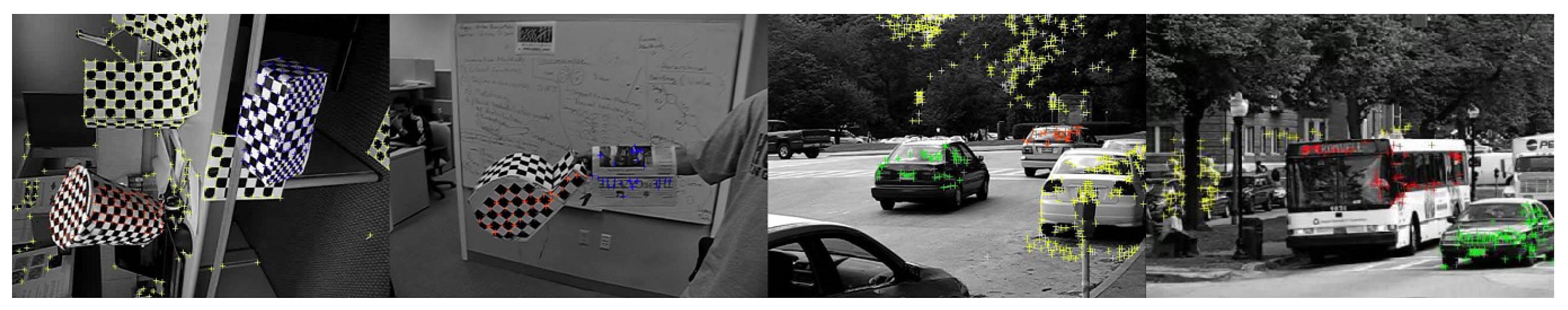
4.4. Motion Segmentation on Hopkins155

In this experiment, we implement motion segmentation to find the independent moving rigid objects by their trajectories. In theory, when a rigid object moves in a video, the points of its trajectories will be formulated as a low dimensional subspace. Thus one can find the moving objects by using subspace clustering technique on the tracked trajectories. From this point, we test our clustering methods on the motion benchmark dataset, Hopkins155, which contains three categories of 156 video sequences with each sequence having two or three moving objects, including indoor objects covered by checkerboard texture, outdoor objects like car, and articulated objects like people. The feature points of the objects are extracted and tracked in all the frames. The ground-truth segmentation is also provided in the dataset for comparison purpose. Some sample images of the dataset are provided in Figure 5. In our experiment, the parameters ${\lambda }_1=800,{\lambda }_2=$ 10,000 for LLE-SSC and ${\lambda }_1=200,{\lambda }_2$ = 10,000 for LLE-LRR.

As there only two or three classes in the experiment, we only report the clustering results in maximal, mean, median and the standard deviation values, as shown in

Table 5. Clustering results on Hopkins 155 dataset. The max value (max), mean value (mean), median value (med) and the standard deviation (std) of the errors are reported on the total 155 motion sequences. The best results are in bold font.

	SSC	LRR	NSLRR	SMR	LapLRR	LLE-SSC	LLE-LRR
max	42.34	41.18	35.06	49.67	46.43	33.89	31.12
mean	3.11	4.83	3.74	5.56	5.36	1.57	1.43
med	0.00	0.52	0.00	0.19	0.24	0.20	0.21
std	7.78	9.35	7.02	10.42	10.41	3.70	3.51

. On the whole, the performances of all clustering methods are quite good as all methods have clustering errors less than 6% in terms of mean. The reason is two fold. The first is that Hopkins155 is a nearly noise-free dataset. The second is that the number of classes is small in this clustering experiment. It is worth noting that our LLE-LRR method has the best result with the mean error of 1.43%.

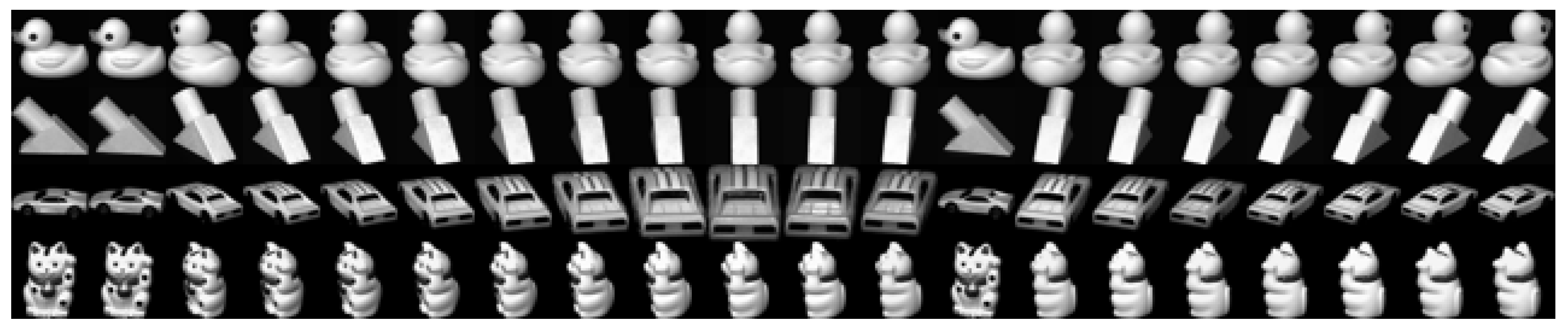
4.5. Object Image Clustering on COIL20

In this experiment, we test the clustering performance of our methods on the object image dataset of COIL20. The dataset contains 32 × 32 gray scale images of 20 objects. The object images are generally captured at different views. Some sample images of this dataset are provided in Figure 6. Here we randomly select $c=[2,3,4,5,6,8,7,8,9,10,11]$ objects for clustering. For each selected object, 36 images are randomly picked up. For each value of c, we run 30 times of clustering by randomly choosing different images for each class and the mean error is reported as the final result. The parameters ${\lambda }_1=100,{\lambda }_2=1000$ for LLE-SSC and ${\lambda }_1=5,{\lambda }_2=2000$ for LLE-LRR.

The clustering results are shown in

Table 6. Clustering results on COIL20 dataset. The clustering errors for $2,3,4,5,6,7,8,9,10,11$ classes and their mean error are shown here. The best results are in bold font.

Number of Classes	The Clustering Error (%)
	SSC	LRR	NSLLRR	SMR	LapLRR	LLE-SSC	LLE-LRR
2	5.32	6.38	2.92	2.13	2.50	3.10	3.33
3	10.59	7.75	9.48	6.98	8.55	5.12	6.42
4	14.05	12.55	10.12	16.89	11.48	7.25	8.87
5	21.70	15.29	15.20	17.18	14.61	10.37	10.89
6	25.31	17.84	16.20	16.03	16.78	16.13	12.38
7	29.07	21.31	20.61	18.54	18.70	16.79	14.06
8	25.63	22.21	24.91	21.64	16.75	16.42	14.53
9	27.54	25.32	24.87	23.69	19.22	23.90	20.93
10	33.21	27.52	25.40	24.09	21.46	18.93	17.60
11	30.21	29.49	28.96	25.27	25.38	26.31	20.72
mean	22.26	18.57	17.87	17.24	15.54	14.43	12.97

. It is shown that our proposed LLE-SSC and LLE-LRR methods still perform excellently in this experiment. Compared with the other methods, LLE-SSC has better clustering results when the classes number is relatively small, while LLE-LRR has better results when the classes number is large. Particularly, LLE-LRR has the best result of 12.97% in terms of mean error.

5. Conclusions

In this paper, we proposed a new data clustering framework based on manifold learning and subspace clustering. Different from the traditional data subspace methods, which try to utilize the data similarity to construct Laplacian graph constraint for data representation. In the proposed framework, LLE is used to learn the manifold structure hidden in the data. The learned non-linear manifold is taken as a regularization for the subspace clustering methods, SSC and LRR, which results in the proposed LLE-SSC and LLE-LRR clustering methods. To evaluate the proposed clustering methods, we implement several clustering experiments on different types of datasets, such as the synthetic data, face images, handwritten digital images, object images and the motion sequences. The experimental results showed that the proposed methods have good clustering performance compared with related methods on different datasets. Particularly, the proposed methods have two advantages. Firstly, from the results of the experiments on the synthetic data with noise, it is shown that the proposed methods are robust to the noisy data. Secondly, from the clustering results on the Extended Yale B, USPS, COIL20 datasets with the number of the clusters increasing, we can observe that our methods show more stability than the compared methods, which means our methods have the potential for clustering a large scale of datasets. These characteristics make them prospective methods in data clustering.

It is shown that using the manifold learning method to reveal the non-linear property of the data and introducing the learned manifold constraint into subspace clustering methods will improve the data clustering performance. However, in this paper, we only use the common used LLE method to verify this idea by integrating it with the classic subspace clustering methods, SSC and LRR. We believe that the developing manifold learning methods are more helpful in dealing with more complicated data in practice. So one of our future works is to exploit a more suitable manifold learning method and integrate it to improve the data clustering performance. The other future work is to extend our methods by parallel computation technique in order to improve their efficiency and make them practical and suitable for clustering large scale data.