Abstract
The harmonic potential field of an incompressible nonviscous fluid governed by the Laplace’s Equation has shown its potential for being beneficial to autonomous unmanned vehicles to generate smooth, natural-looking, and predictable paths for obstacle avoidance. The streamlines generated by the boundary value problem of the Laplace’s Equation have explicit, easily computable, or analytic vector fields as the path tangent or robot heading specification without the waypoints and higher order path characteristics. We implemented an obstacle avoidance approach with a focus on curvature constraint for a non-holonomic mobile robot regarded as a particle using curvature-constrained streamlines and streamline changing via pure pursuit. First, we use the potential flow field around a circle to derive three primitive curvature-constrained paths to avoid single obstacles. Furthermore, the pure pursuit controller is implemented to achieve a smooth transition between the streamline paths in the environment with multiple obstacles. In addition to comparative simulations, a proof of concept experiment implemented on a two-wheel driving mobile robot with range sensors validates the practical usefulness of the integrated system that is able to navigate smoothly and safely among multiple cylinder obstacles. The computational requirement of the obstacle avoidance system takes advantage of an a priori selection of fast computing primitive streamline paths, thus, making the system able to generate online a feasible path with a lower maximum curvature that does not violate the curvature constraint.
1. Introduction
Due to advances in sensing, actuation, communication, computing, storage, and AI technologies with affordable costs, increasing deployment and applications of intelligent autonomous mobile robots or ground vehicles for long-term operation are prevalent. The integrated platforms at our disposal are intended for missions such as SAR (search and rescue), autonomous driver-less driving, manufacturing, and surveillance in cluttered environments [1,2,3,4,5,6,7,8,9,10,11,12,13,14,15,16,17,18,19,20,21,22,23,24,25,26,27,28,29,30,31,32,33,34,35,36,37,38,39,40]. Along with an increasingly heavy interaction between human and robots, update-to-date but cost-effective implementation or prototyping of intelligent mobile robot systems to accomplish missions autonomously employing recent advances in localization, mapping, and navigation have been the focus of some endeavors put into the robotic systems, as shown, for instance, in References [39,41,42,43].
Obstacle avoidance and motion planning [2,3,4,31] are essential for the completion of missions in a smooth and optimal manner. A variety of obstacle avoidance algorithms are designed and implemented for navigating a mobile robot to avoid static and dynamic obstacles in open space or in narrow passages. The artificial potential field (APF) approach is one of the most well-known reactive online obstacle avoidance methods applicable in known or unknown environments [5]. The goal position of the robot is assigned as an artificial attractive potential and obstacles are applied as artificial repulsive forces. Then, the collision avoidance path is derived by using the gradient of the linear superposition of each potential. However, by following the gradient path of APF, navigation routes generated by APFs suffer from the local minima due to the presence of obstacles, i.e., the set of trap positions where the gradient of APF vanishes so that the robot gets stuck there, thus preventing the robot from reaching the target or lower the navigation efficiency. The number of obstacles affects the number of local minima significantly [44]. In general, it is desired that no other local minima except the goal exist in APF so that the navigation is efficient. For this purpose, hydrodynamic or harmonic (or velocity) potential functions (HPFs) (see References [7,9,15,17]) derived from the velocity potential of the solution to the boundary value problem of Laplace’s Equation with appropriate boundary conditions in a computational domain are proposed as an appealing class of APFs for navigation. The properties of HPFs such as min-max principle and superposition in the context of path planning were proved in the foundation work [7,15,17]. To ensure the repulsion of the flow from the obstacles, one effective way is to impose two types of boundary conditions on the obstacle and domain boundaries for the solution to the Laplace’s Equation in a computational domain: Dirichlet type (the potentials on the boundaries of obstacles and domain are assigned a constant high value, i.e., the fluid motion on the obstacle boundary is along the normal direction of the obstacle boundary/wall) and Neumann type (i.e., the flow cannot pass through the boundary, or the fluid motion on the obstacle boundary and wall is parallel to the tangential direction of the obstacle boundary since the normal component is null). For path planning, the HPF has the property of the min-max principle, so that no local minima other than the goal in the interior of cluttered or bounded environments with state constraints of a point robot are defined by Dirichlet boundary conditions or Neumann boundary conditions on the borders of the obstacles and computational domain.
Motion planning based on hydrodynamic potential applies (1) different fundamental elements such as a point sink (representing the goal), a point source (representing the robot location), or a uniform flow (defined as a flow with constant speed in a prespecified direction) plus a doublet (representing the obstacle), and their superposition, or (2) velocity potential solution to the Laplace’s Equation with appropriate boundary conditions, to create a new HPF. The gradient of the HPF or the streamline that defines the vector field of the path at every point can be computed efficiently; analytically for a simple obstacle shape such as a circle or numerically. There are a few simulations showing that a vehicle modeled as a point (fluid) particle could smoothly navigate without collision with the (circular, elliptical, rectangle, or arbitrary-shaped) obstacles [6,8,11,12,13,14,15,16,17,18,26,30] by following streamlines from a variety of start points in an environment composed of multiple obstacles. To build an APF via hydrodynamics potential, Reference [15] proposed a panel method by first approximating an arbitrarily shaped obstacle by an enclosing polygon (set of panels). Each obstacle panel is treated as a source/sink with the strength adjusted to make the obstacle a repelling potential function by summing the HPF of each panel, i.e., with nonzero outer normal velocity at the obstacle panel representative point. Wang et al. [16] introduced a reactivity parameter to adjust the amplitude of the path’s deflection around an obstacle and an optimal 3D path is obtained by a genetic algorithm. For path planning on an unstructured terrain consisting of meshes of different size and geometry of computational domain discretized by finite element, Reference [25] proposed to use a graph search to generate an initial path from the start to the goal, then used streamlines to smooth the initial path.
Planning and optimization of state and input trajectories for stabilizing non-holonomic mobile robots studied in this paper or more general non-holonomic systems such as a car with trailers [33] in multiple obstacles environment subject to bounded state constraints (such as the environment constraint and path and its derivative constraints) and input constraints is challenging. The motion planners have to plan in the full state space (the space of position, heading, speed, curvature, and/or curvature derivative) and deal simultaneously with constraints of collision avoidance and non-holonomic constraint and admissible input (such as the computation of the invariant set or reachable set of the system [31]). Approaches that can either achieve the optimal or near-optimal position and heading and velocity or higher order derivatives simultaneously or sequentially are proposed for non-holonomic mobile robots. A dipolar potential field is combined with discontinuous state feedback for navigating a non-holonomic mobile robot in the presence of obstacles in Reference [32]. Pontryagin Maximum Principle in variational form was employed in Reference [33] to obtain a convergent sequence of controls for optimal motions of general non-holonomic systems with state and input constraints. New methods to non-holonomic path planning are given in Reference [34], which proposed to steer the non-holonomic mobile robot without additional constraints via rotation and linear translation using trigonometric switch inputs, a generic APF-based method via deforming a feasible path of non-holonomic systems (e.g., a mobile robot with trailers) without the violating non-holonomic constraint [35], and the ones based on partial differential equations other than the Laplace’s Equation coined by References [7,24], which applied a parabolic partial differential equation, and Reference [29], which used the Navier–Stokes equation of viscous flow for path planning. It is noted that HPF is interpreted in heat conduction, instead of hydrodynamics, in a recent work [28] with a demonstration of a real-time mobile robot navigation experiment.
To produce a feasible path that avoids obstacles in a cluttered environment, waypoint navigation method has been a viable approach used to generate a sequence of waypoints connected via a path primitive [36,37] for reactive trajectory generation, while the entire path satisfies the smoothness requirement or some other criterion and respects the kinodynamic constraints imposed on the vehicle motion such as the constraints on the instantaneous velocities that can be achieved [2,22]. However, the path primitives have to be recomputed whenever some of the waypoints built between the start and the goal are changed. Furthermore, the entire path could be lengthy because of many detours. HPF-based non-holonomic path planning for a mobile robot subject to kinodynamic constraints [17,22,26] takes advantages of features of streamlines that are very appropriate for building a directional navigation system:
- (i)
- Streamlines are rich, thus, enabling the selection of appropriate paths for the planner. The desired state trajectory to be followed by a robot is determined only by the input defined by HPFs, i.e., along a streamline-based trajectory compatible with the kinodynamic constraints of the motion, even in high-speed motion [12].
- (ii)
- In many applications, the smoothness of trajectories is essential. Trajectories generated by HPF approaches are the integral curves of the gradient vector field of HPF. The trajectories that are smooth are readily executable.
- (iii)
- Streamlines can be computed offline systematically based on prior obstacle information (distribution, i.e., shape, size, location, and number) without the waypoints and path primitives, thus, being more predictable.
- (iv)
- Notably, the HPF-based path planner is a complete [7] and anytime algorithm [10], in which the streamlines generated cover the free regions of the workspace.
Lau et al. [18] provide a streamline-based kinodynamic motion planning approach to avoid elliptical obstacles, guaranteeing that both velocity and curvature are within limits by adjusting the strength of a source and a sink if a portion of the 3D trajectory violates the kinematic constraints. Recent work [26] used the gradient of HPF as an additional input to alter the motion pattern of a two-wheeled drive mobile robot based on the stabilizing controller design using an invariant manifold to avoid the obstacles, thus, extending the guidance method of Reference [22] based on the HPF only. Along this line of HPF-based non-holonomic path planning work, this work starts with the point that the curvature constraint, viewed as a constrained input to (1), significantly restricts the selection or generation of allowable paths to be followed in a cluttered environment. We elaborate on demonstrating the potential of the hydrodynamics-based motion planning approach of (1) subject to the curvature constraint. An obstacle avoidance system using three primitive streamline-based paths and a path selection strategy that makes the avoidance of small obstacle easier is proposed. For avoiding multiple obstacles, a pure pursuit algorithm [20,21] is implemented in this paper for the purpose of enabling a smooth and safe transition using streamline changing between obstacles without violating the curvature constraint. The experiment is conducted for a constant speed circular non-holonomic mobile robot to navigate smoothly in real-world partially unknown environments cluttered with cylinder-shaped obstacles. The Dr. Robot X80 robot (Dr Robot Inc. in Markham, ON, Canada), which was equipped with a low-cost sonar and infrared sensors to detect obstacles during motion, is used as the navigation platform.
The paper is organized as follows. Section 2 gives a brief introduction of a mobile robot with two independently driven wheels for the experiment. Section 3 mentions the harmonic potential field approach for avoiding cylindrical obstacles. Then, we propose three primitive paths based on streamlines and a distance-based path selection strategy of a primitive path for obstacle avoidance of curvature-constrained non-holonomic mobile robots. In Section 4, we propose a new real-time obstacle avoidance system using primitive paths and streamline-changing via the pure pursuit algorithm. Comparisons and the proof of concept experimental result in a simple cluttered environment are presented in Section 5. Section 6 ends with the conclusions of the paper.
2. The Mobile Robot with Range Sensors
2.1. Wheeled Mobile Robot System
We implemented our real-time hydrodynamics-based obstacle avoidance algorithm on Dr. robot X80, a wireless two-wheeled drive mobile robot platform. Figure 1 shows the configuration and the front view of the mobile robot. The X80 mobile robot is an integrated electronic and software robotic system. It can be designed through a set of ActiveX control components (SDK) developed for C/C++. A DUR5200 Ultrasonic Sensor and GP2Y0A21YK Sharp Infrared Sensor are equipped on the mobile robot. The robot platform is further modified to be equipped with a laser scanner, Kinect, and a laptop. The navigation algorithm runs directly on the remote PC through wireless communication.
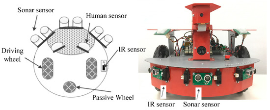
Figure 1.
The outline of the circular non-holonomic mobile robot Dr. Robot X80 used for the experiment.
2.2. Kinematic Model
Figure 2 illustrates the kinematic model of the differential-drive circular mobile robot with radius rRobot. The mobile robot is modeled as a representative point of the circular mobile robot so that its non-holonomic constraint of rolling without the slipping of wheels is described by the kinematics of the non-holonomic unicycle (1).
where (x, y) denotes the coordinates and θ denotes the orientation (heading), and denote the velocity and angular velocity, respectively. As long as the velocity vector is tangent to the path the unicycle follows, the non-holonomic constraint (1) is automatically satisfied. The non-holonomic constraint (1) limits the maneuverability of the vehicle motion so that no instantaneous lateral motion is allowed. The mobile robot is controlled by the low level velocity control of two wheels driven by DC motors independently. The velocities of the mobile robot are determined by the actuated wheel velocities via the one-to-one correspondence given by
where and denote the left and right wheel velocity, respectively; r is the wheel radius; d is the distance between the two wheels.
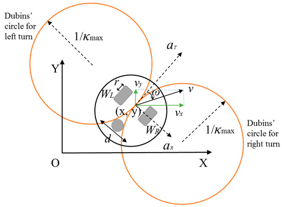
Figure 2.
The mobile robot’s kinematic model with the curvature constraint, where a positive curvature denotes a right (clockwise) turn. The robot is assumed as a circle. The robot velocity U and its x-component vx, y-component vy, the radial acceleration aR, and tangential acceleration aT, are shown. The O-XY coordinate system is the global coordinate frame and a local frame is attached to a representative point (the center) of the circular mobile robot.
2.3. Obstacle Detector
Obstacle avoidance relies on the detection of obstacles for the real-time operation of mobile robots. The sensor configuration is shown in Figure 3. A DUR5200 Ultrasonic Sensor and GP2Y0A21YK Sharp Infrared Sensor are equipped on the mobile robot. There are three sonars (Sonar 1, Sonar 2, and Sonar 3) and four infrared sensors (IR 1, IR 2, IR 3, and IR 4) on the mobile robot, where θ1 equals 12°, θ2 equals 18°, and θ3 equals 15°. The detecting range of an ultrasonic sensor is from 4 to 255 cm, while the detecting distance range of the IR sensor is between 10 and 80 cm. The sensors’ update rate are both 10 Hz. We assume the obstacle is located in the direction of the sensor if only a single sensor detects an obstacle. Otherwise, when two sensors detect an obstacle at the same time, we assume that the obstacle lies on the bisector of these two sensors’ directions. Figure 4 shows the detection of an obstacle. For instance, if Sonar 2 detects an obstacle, the obstacle is located in front of the robot with an azimuth angle 0°. Likewise, Sonar 1, Sonar 3, IR 1, IR 2, IR 3, and IR 4 detect the obstacle with azimuths of 45°, –45°, –30°, –12°, 12°, and 30°, respectively. If both Sonar 2 and IR 3 detect an obstacle, then the obstacle’s direction will be 6°, which is between Sonar 2 and IR 3. The estimated obstacle location is transformed into the global frame for the motion planner. The estimation and localization errors are accommodated by a safety distance rSafe in the practical implementation of the navigation system, as in our experiment presented in Section 5.
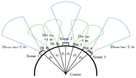
Figure 3.
The configuration of the sonar and infrared sensors and their sensing ranges in Dr. Robot X80.
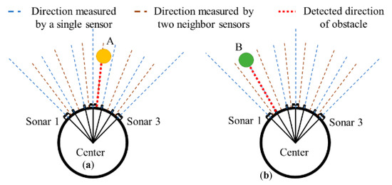
Figure 4.
The scenarios of obstacle detection. The ray of each sensor is presented as a dashed line. As the rays intersect with an obstacle, the nearest intersection point is retained. (a) An obstacle is in front of the robot. Sonar 2 detects an obstacle with distance less than 150 cm, the robot knows the obstacle is located in front of the robot with azimuth angle 0°. (b) Both Sonar 2 and IR 3 detect the obstacle, and the obstacle’s direction will be 6 °, which is between Sonar 2 and IR 3. The distance of the obstacle is the average of the data received from the two sensors.
3. Obstacle Avoidance Model by Harmonic Potential Field with Curvature Constraint
Extracting the topologically different candidate trajectories from a set of trajectories based on the equivalence relations and optimization schemes is a means of efficient online local trajectory optimization [44]. To provide a collision-free path rapidly to the planner, it is beneficial to extract a priori the streamlines that specify the essential motion pattern details of desired navigation trajectories such as curvature constraint and free of multiple local minima. In this section, we briefly summarize the smooth path produced by the streamlines of the harmonic potential field. Then we present a mobile robot navigation system based on the streamlines of HPF that satisfy the curvature constraint. The system is based on three primitive paths extracted from the streamlines and pure pursuit algorithm for streamline-changing.
3.1. Harmonic Potential Function and Streamlines
Harmonic potential functions are solutions to Laplace’s Equation, so functions generated by Laplace’s Equation do not exhibit local minima [7]. In a two-dimensional computational domain of Euclidean space, the velocity potential is a solution of Laplace’s Equation with the given boundary conditions that govern the flow of the non-viscous, incompressible, irrotational fluid particle motion at every point of the domain. Laplace’s Equation can be solved analytically in simple cases or by numerical methods in a general situation. For numerical methods, Laplace’s Equation in a computational domain could be discretized using both the finite difference method or the finite element method, resulting in a system of linear equations for the solution of the potential value in a grid or mesh environment. The Jacobi iteration, Gauss-Seidel iteration, and SOR (successive over-relaxation) iteration methods in a grid environment can be employed to solve the linear equations with an efficient accuracy. A log-space algorithm with GPU acceleration was proposed to fix the numerical precision problem of the numerical solution of a linear system of linear equations at the grid points that have nearly vanishing gradients resulting from discretized Laplace’s Equation via the finite difference methods [10]. A streamline indicates the local flow direction: its tangent at every point (vector field) is in the direction of the local fluid velocity associated with the flow defined in Equation (2).
That is, the gradient of the obtained potential values gives the streamline or the direction of velocity at each grid [7], offering an explicit specification of the heading of a smooth, natural-looking path for navigation. Higher order path characteristics such as curvature can also be obtained for streamlines, thus, being more predictable.
Consider a mobile robot at x = [x y]T modeled as a fluid particle moving with velocity in the Cartesian space. It moves in the +x-axis direction with a forward/longitudinal speed U to avoid a circular obstacle of radius rObstacle (or an enlarged rObs for safety) located at the origin. The velocity potential field can be represented as the superposition of a uniform rectilinear flow and a doublet [19] as
where . According to [19], the robot’s velocity in the Cartesian coordinate is determined by the gradient
In practice (and in our experiment in Section 5), we assume that the linear speed is normalized to unity while its direction of motion is preserved. Then, the normalized velocity and the corresponding acceleration of each point on the streamline in the uniform flow are given by (5) and (6).
Furthermore, curvature and deviation of curvature can be derived by velocity and acceleration as
From the above equations, given a start position and a circle with a known radius at the origin, a streamline (integral curve) can be derived by numerical integration of the velocity vector field that specifies the tangent of the path or the robot heading at each point. In addition, the higher order path characteristics such as curvature are easily computable as well, making the path to be followed more predictable. That is, the velocity vector field of streamlines serves as a vector field for the guidance of the robot’s motion everywhere in the obstacle-free region. Therefore, in path planning applications, streamlines provide a pool of systematic paths that have an explicit or analytic vector field for the tangent to the path as the path specification, and their higher order path properties such as curvature could be easily computed as well. However, there are several drawbacks for robots to purely follow streamline paths. First of all, we assume that the curvature of unicycle kinematics (1) is constrained by its upper bound. The curvature of streamline it follows has a larger curvature as the distance to the obstacle gets closer. For example, Figure 5 depicts that streamline starting from (−5, 0.2) exhibits the maximum curvature. Second, the paths with a smaller curvature are longer and keep an unnecessary distance with the obstacle. Moreover, for paths with an initial position further than the radius of the obstacle in the direction of the x-axis, it is not necessary to follow a streamline path because a robot can pass the obstacle straightly, such as the paths with a start position further than the radius of obstacle with the x-axis in Figure 5. Therefore, we provide an improved streamline-based approach in the following section.
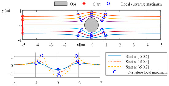
Figure 5.
The streamline paths (upper plot) with different start positions and their curvatures (lower plot) for a uniform flow around a circular obstacle. The path to avoid an obstacle is similar to the streamline of the fluid flow around a cylinder. The very large turning radii of some of the paths closer to the obstacle may become infeasible when the curvature constraint imposed on the vehicle motion is accounted for.
3.2. Three Primitive Paths with Curvature Constraint
In Figure 6 we show a scenario of three alternative options in which another obstacle is encountered immediately after circumventing one obstacle. Therefore, the robot has to turn sharply to prevent an imminent collision, as shown in Figure 6a. On the other hand, passing the first obstacle with a low curvature streamline allows the robot to pass these two obstacles from the same side while there is not enough space to pass through between the two obstacles using a streamline and complying with the curvature constraint, as shown in Figure 6b. The third way shown in Figure 6c is passing the obstacle from the farther side by a sharp turn. The example demonstrates that the different timings for applying these two strategies are related to the upcoming obstacle’s position after passing the first obstacle.
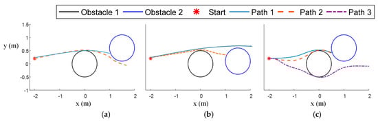
Figure 6.
Sequential obstacle avoidance via sharp turn and low-curvature turn in the situation of different obstacle configurations (a) From the space between two obstacles; (b) From the same side of both obstacles; (c) From farther side.
There are two strategies for local obstacle avoidance based on streamlines. For local obstacle avoidance, a point robot could circumvent an obstacle from its left or its right side. Alternatively, it could also pass an obstacle with maximum curvature via a sharp turn. We first describe the three primitive paths for the avoidance of a single circular obstacle. For multiple obstacles, the same strategy is employed sequentially for every detected obstacle that is to be avoided. The following are the details and procedures of a sharp turn and low curvature turn for avoiding the obstacle by using streamline paths. Three collision-free primitive paths most aligned to the current robot’s heading that achieve compliance with the curvature constraint of the mobile robot are proposed by exploiting the richness of the streamlines that cover the computational domain of Laplace’s Equation and the rather intuitive property that the deflection and curvature of a streamline become smaller as it is farther from the obstacle. For simplicity of illustration, we refer to Figure 7. It is assumed that the robot is moving in the +x-direction and a circular obstacle of radius is located at the origin so that the maximum curvature of streamline occurs at the y-axis.
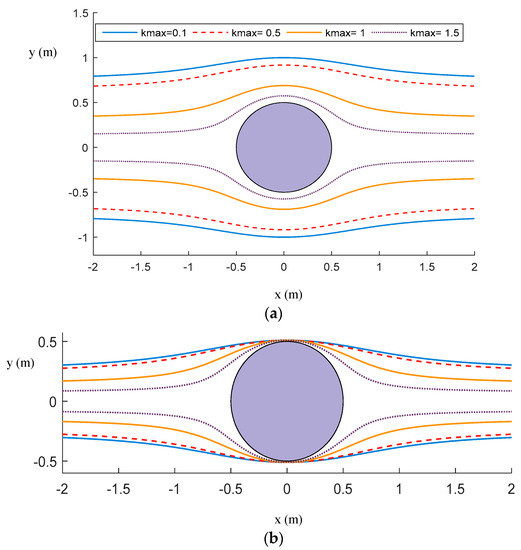
Figure 7.
The concept of sharp turn streamline paths to circumvent a circular obstacle with the center placed at the origin in the x-y plane. (a) Streamline paths with different maximum curvatures. The curvature of the streamline is larger as it is closer to the circle. (b) Feasible paths compatible with different curvature constraints are pulled back to graze the obstacle border.
(A) Continuous-curvature sharp left or right turn
Consider the avoidance of the nearest obstacle within the sensing range in front of the robot. Two curvature-constrained streamline-based left or right turn paths could be used as two primitive paths to ensure the safe navigation from the left or right side of the obstacle based on the obstacle’s radius. In particular, we look for the two streamlines corresponding to the left turn and right turn with a curvature maximum equal to the maximum curvature . The desired streamline is obtained by shifting the selected streamline in a parallel way until its curvature maximum point grazes the obstacle boundary.
Figure 7 illustrates an example of a hydrodynamic streamline path with different curvature constraints. From the curvatures of flow depicted in Figure 7a (similar to the scenario of Figure 5), if the initial y-position is further away from the center of the obstacle, a collision-free path is a nearly straight streamline with a smaller curvature. In addition, we identify that the points with local maximum curvature on a streamline are located at the y-axis, assuming that for simplicity the robot is moving forward in the x-direction. In order to verify the curvature constraint for a streamline path, the points of maximum curvature of a streamline have to be found so that it is sufficient to search over the streamlines that satisfy the curvature constraint. In the scenario depicted in Figure 7, the maximum curvature of a streamline path is smaller when further from the obstacle, and there are two points with a local maximum curvature in a single path. They lie on the y-axis and are identified first by a binary search presented in Algorithm 1. Algorithm 1 starts with a point with curvature (7) not larger than the maximum
This point with the largest magnitude || is identified by increasing the y coordinate from the upper-most border point (0, a) of the obstacle centered at (0, 0) with radius a. Then, Algorithm 1 of binary search is used to locate the point between and with a curvature equal to the maximum allowed curvature . Then, the streamline path is generated with a velocity U in (5) by numerical integration initialized with . In this way, we can find two streamlines with a given maximum curvature with starts at a different location from the current robot position. The streamlines in the region between do not comply with the curvature constraints. The modified streamlines obtained by pulling the streamlines back to the current robot position are the paths, as shown in Figure 7b.
| Algorithm 1.Bisection for searchingyLow_max, yLow_min |
| Input: Maximum allowed curvature , a circular obstacle with center (0,0) and radius a Output: Maximum curvature point y in the y-axis and its curvature //First find (i) yLow_max whose curvature is not larger than then find (ii) yLow_min whose curvature is . While // endwhile //Curvature maximum point is found by binary search on the interval [yHigh,yLow] While //ε: tolerance If then yLow = y Else yHigh = y end if end while return y |
(B) Continuous-curvature low curvature turn
Among the possible streamlines that can pass a given obstacle in front of the mobile robot, a feasible path with a low curvature using Algorithm 1can be found. This is done by using Algorithm 1 for searching the unique streamline passing with the largest || satisfying Equation (9). This streamline is called the low curvature turn path. A low-curvature collision-free path is found by Algorithm 1, a lateral displacement vertical to the moving direction (as Figure 8 shows, along direction) is used to pull the low curvature streamline path back to the current robot position. Figure 8 shows the concept of the low curvature path.
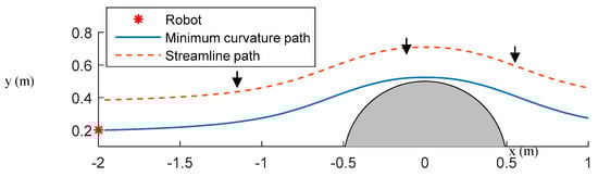
Figure 8.
The concept of the low curvature path.
Given an obstacle’s radius and the robot’s maximum allowed curvature, we can derive three primitive paths which satisfy the curvature constraints as described above. For all three primitive paths, the robot needs to keep a sufficient longitudinal distance with the obstacle to achieve the pursuit of the primitive paths with a stricter curvature constraint, i.e., a lower maximum curvature. In addition, while the maximum curvature constraint decreases, it is more difficult to achieve primitive paths. Excessively restrictive curvature constraint causes no feasible path is found. Moreover, the lateral distance to the obstacle will influence the ability to find a feasible path. Figure 9 demonstrates primitive paths correspond to various initial positions (or relative distance to the obstacle) and curvature constraints.
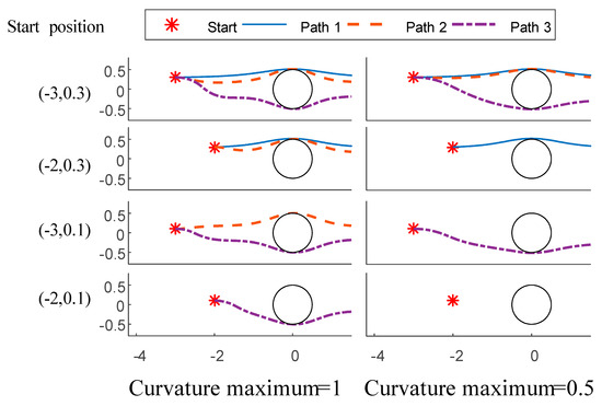
Figure 9.
The single obstacle avoidance path for different start positions and the curvature maximum constraint in the x-y plane. The radius of the obstacle is 0.5 m. The robot forward moving direction is the positive x-axis (toward the right).
3.3. Distance-Based Obstacle-Avoiding Path Selecting Strategy
The selecting strategy of quickly computing three primitive streamlines has to identify the situation the robot encounters, depending on the reaction distance to the upcoming obstacle position or lateral displacement relative to the size of the obstacle. The strategy is illustrated in the scenario of Figure 10. The robot is initially located at x = −2 with a different lateral distance y related to a cylindrical obstacle at the origin. Let b+ and b− be the points which two sharp turn paths intersect with the line x = −2. The interval [−r, r], denoted by [d−, d+] in Figure 10 at the vertical line x = −2 is partitioned into intervals B+~B− by the labeled points d− to d+ according to the start points of the primitive paths, symmetrically with respect to the current robot position. We define Lsharp as the distance between points c+ (the start point with a right sharp turn path) and c− (the start point with a low curvature path).
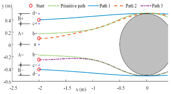
Figure 10.
The illustration of the primitive path selecting strategy. The range [−, ] according to the obstacle size is partitioned manually into three intervals from far to near to reflect the reaction distance. Robots with different lateral displacements related to an obstacle will pursue different primitive streamline paths aligned with the current robot heading. Path 1 and Path 2 tangentially traverse the enlarged circular obstacle boundary.
Specifically, given a current robot configuration and an obstacle of known size and location in front of the robot forward route, we propose the following rules
The strategy is according to the relative lateral distance measured from the center of the obstacle (, in front of the robot, where the current robot location is at a fixed longitudinal distance. The range [−,] according to the obstacle size is partitioned manually into three intervals from far to near to reflect the reaction distance as Figure 10 shows. Once an obstacle is sensed by the obstacle detector, the motion planner determines the proper primitive path via Equation (9) for the mobile robot to follow to circumvent the obstacle. This strategy is designed to use a low curvature turn in Intervals A+ and A−, while it pursues a sharp left turn in Interval B+ and a sharp right turn in Interval B− as the obstacle is closer. In addition, this strategy makes the avoidance of a small obstacle easier (with smaller ). Note that for obstacles with the same radius, the paths generated by streamlines of Laplace’s Equation according to the same position are identical. Hence, a set of streamline paths can be a priori computed for circular obstacles with different radii and stored and maintained in the dataset. The path obtained by transforming a sample path computed for an obstacle located at the origin to the estimated or true obstacle position could then be re-used to online plan or re-plan the collision-free movement with a reduced time-complexity. In practice, the localization error requires the motion planner to online update the primitive path according to a proposed lateral distance-based path selection strategy.
4. Real-Time Streamline-Based Obstacle Avoidance Strategy
4.1. Overview of the Obstacle Avoidance System
Figure 11 depicts the building blocks of the obstacle avoidance system. The real-time obstacle avoidance system is built by three subsystems, which are the obstacle detector, the motion planner that incorporates the curvature constraint, and the pure pursuit controller used to control the robot to follow the specific primitive path with an allowable angular velocity satisfying the curvature constraint. For the part of the robot’s hardware, we used the robot’s kinematic model to estimate the robot’s own kinematics and the sensors to detect the surrounding environment. The obstacle’s global location is estimated by the range data received from sonar and infrared sensors. Our motion planner initially selects a streamline starting from the robot’s start position, which is generated based on an a priori known obstacle distribution. The obstacle’s location is updated based on new sensor data during the robot’s forward motion, and the motion planner will decide whether to enable local re-planning based on a path selection strategy or to retain the original path for the robot to follow. Local re-planning is performed by generating and updating a local subgoal that is on a new primitive collision-free path and the smooth transition between streamlines is enabled via pure pursuit.
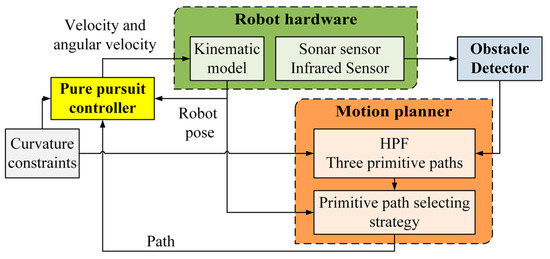
Figure 11.
The flowchart of the online obstacle avoidance system for a curvature constrained non-holonomic mobile robot based on the primitive streamline paths, a path selection strategy, and a pure pursuit algorithm for streamline changing.
4.2. Pure Pursuit Controller for Mobile Robots
We assume that an initial streamline is chosen based on the initial robot configuration and an a priori known obstacle distribution, taking into consideration the curvature constraint. This initial path may collide with obstacles. To ensure the safe and smooth navigation, one subsystem of our obstacle avoidance system in Figure 11 is to make the robot redirect from following one streamline to an alternative streamline at a look-ahead distance via a local, online pure pursuit algorithm without violating curvature constraint. Figure 12 shows the plots of a streamline-changing circular path for redirecting the mobile robot from its current pose to a subgoal on another streamline via pure pursuit. The details are as follows.
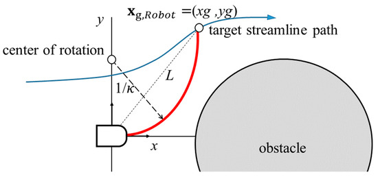
Figure 12.
The smooth transition for redirecting the mobile robot from its current pose on current the streamline to a subgoal on the target streamline via pure pursuit.
Pure pursuit is a path tracking method by calculating the curvature of a new circular path for a vehicle to pursuit a subgoal position ahead of the vehicle by leaving the initially planned path from its current position [20,21], where the orientation of the subgoal is not concerned. Due to the fact that non-holonomic mobile robots cannot directly move in the lateral direction, a robot pursues a subgoal position ahead of the robot to redirect from its current position along an arc of curvature via pure pursuit. Since the obstacle avoidance path can be computed analytically according to the relative position of the robot and obstacle and shape and size of the obstacle, this method has an implementation advantage.
Once a streamline is selected for streamline-changing, the next step is to find a subgoal point Xg which is located after the closest point in the global coordinate. Let a local coordinate system be attached to the robot with its origin set as the rotation center of the robot and the +x-axis of the local frame aligned with the forward motion direction. Then transform a subgoal point Xg in the global coordinate to xg,Robot = [xg yg]T in the local frame with xg and yg denoting the longitudinal and the lateral displacements, respectively:
where XRobot is the current robot position in the global frame, and is the heading angle of the robot in the global frame. The subgoal point xg,Robot in the vehicle coordinates can be represented with curvature and by geometry:
where is the angle of the arc between the vehicle and the subgoal (see Figure 12). The subgoal point to pursue keeps a specific look-ahead distance , since non-holonomic robots cannot correct errors directly with respect to the nearest point on the path.
Now the equations of the pure-pursuit curvature control law are derived. The curvature of the vehicle is defined as the inverse of the distance , also called the radius of curvature, between the vehicle’s frame origin and its instantaneous CoR (center of rotation). Second, the curvature also represents the instantaneous change of the vehicle heading angle with respect to the traveled distance ds. Hence, curvature is formally defined as follows:
In implementation, curvature can be defined as the instantaneous change of the heading angle with respect to the travel distance in one sampling time . Curvature then could be further related to the robot’s velocity and angular velocity. Therefore, the angular velocity of a robot moves along a path at a constant forward speed could be computed from the path curvature via the following relation (Equation (12)):
where [20]. To satisfy the maximum allowable curvature, we regularize the signed curvature as
Thus, the motion in the local frame of the robot can be applied to command the motion controller via the inverse kinematics of Equation (1). The displacement in the global frame can be derived by exploiting the displacement in the local frame
A pure pursuit algorithm summarizing this subsection is shown in Algorithm 2.
| Algorithm 2. The pure pursuit streamline path. |
| Input: robot initial pose, target streamline path, look-ahead distance, maximum allowable curvature Output: status, pursuit path While (not timeout or status) do let represent the transformation to robot coordinate pClosest← {(x, y)|min{|(x, y)–poseRobot|} and (x, y) in pursuitpath} ← {(x, y) | min{|(x, y) − pClosest|} and (x, y) in pursuit path after pClosest} (9) Calculate the curvature ← Regularize the curvature constraints (Equation (14)) Set the steering angle of the robot (Equation (13)) Update robot’s heading direction, poseRobot if poseRobot and curvature == streamline path do status←TRUE store path into pathArray if collide with obstacle do status←FALSE end while |
4.3. Setting Lookahead Distance
Look-ahead distance is the only parameter in the pure pursuit algorithm, and the reason for the look-ahead distance is that non-holonomic robots cannot correct errors directly with respect to the nearest point on the path [20]. The pure pursuit procedure is summarized in Algorithm 2. The common practice for setting look-ahead distance takes into consideration its effect on path geometry and tracking performance. A longer look-ahead distance results in smoother paths but a worse tracking accuracy. In contrast, a shorter look-ahead can reduce tracking errors more quickly. Yet, due to the curvature constraint, the pure pursuit controller may not be able to follow steering commands, and the robot motion becomes unstable. Therefore, a suitable look-ahead is needed for both stability and tracking performance.
Figure 13 illustrates that the pure pursuit path is sensitive to the setting of look-ahead distance. In this example, there is an angle between the x-axis and the line connecting the point robot and the obstacle center. The path with a look-ahead of 0.5 m has an effective and efficient tracking ability. However, the path with too large of a look-ahead distance, 1 m, for example, is smoother but unable to track the path accurately. On the contrary, the path with a shorter look-ahead 0.1 m responds to tracking errors quickly, but the robot’s motion is unstable and overdamping because of the curvature constraint. Both paths obtained with a look-ahead of 1 m and 0.1 m lead to a collision with the obstacle.
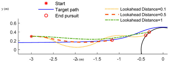
Figure 13.
Replanning via pure pursuit paths starting at a fixed position with a set of subgoals determined by different look-ahead distances. The pursuit paths with look-ahead distance 0.1 and 1 intersect with the obstacle, while the pure pursuit path with a look-ahead distance of 0.5 is collision-free.
4.4. Multiple Obstacles Avoidance Strategies
In an environment composed of multiple obstacles, previous researchers provided several different methods to create a guidance vector field. The weighted superposition of a single obstacle is the most commonly used method for multiple obstacles (e.g., Reference [6,8,11,12,15,18]). Though the sum of HPFs is also HPF (hence, free of local minima), the superposition has no guarantee to satisfy the curvature constraint. Hence, we propose a new avoidance strategy for multiple obstacles.
(1) Superposition of multiple obstacles
A weighted velocity field of each obstacle vector field not only guarantees no local equilibria in the workspace, but also satisfies the zero Neumann boundary condition on every boundary of an obstacle. In multiple obstacles, the path tangent or vector field at each point corresponds to the streamline of the flow with velocity defined by the weighted superposition of velocity which is induced by an individual obstacle. The total influence of all obstacles in an environment with obstacles on the velocity field can be expressed as the weighted sum of of for each obstacle
where is the position-dependent weighting function for obstacle i. One can design with denoting the shortest distance between the robot and the obstacle i. This design makes the closest obstacle have the largest weight. In real-time applications, Equation (16) is calculated for only all of the obstacles detected within the sensing range or a user-defined safety zone.
(2) The proposed strategy
We identify three primitive paths once the robot’s initial pose, maximum allowable curvature, obstacle’s position, and radius are given. Figure 14 summarized the discussions so far as a flowchart of hydrodynamic path planning in combination with pure pursuit in a multiple obstacles situation. In the multiple obstacles situation, we initialize a queue called poseRobotArray to store the robot’s initial pose. While the queue is not empty, we assign the first element of poseRobotArray to poseRobot and pop the first element of the queue. Then, we move the robot forward to the target to check whether the path is collision-free. If no obstacles are detected on the path, we store the path into pathArray. Otherwise, we generate three primitive paths to avoid the detected obstacle. For each generated path, we check if it collides with any other obstacle. If it is still collision-free, we store the robot’s final pose into poseRobotArray. On the other hand, we check if the collision happened before or after passing the first obstacle. If the collision happened before the first obstacle, we generate three primitive paths to avoid the new obstacle from the robot’s initial pose. In contrast, we set the location of the closest point on the path to the original obstacle as poseRobot and then avoid the new obstacle. Finally, we select the optimized path from pathArray.
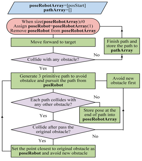
Figure 14.
The flowchart of sequential obstacle avoidance by the hydrodynamic path planning with pure pursuit in the multiple obstacles situation.
5. Comparisons and Experiment
In this section, we demonstrate the proposed algorithm for navigation within multiple circular obstacles via comparisons with other methods to show the planner’s performance in a cluttered environment and a proof of concept experiment to show the feasibility. The speed of the robots was set as 1 m/s for all scenarios and the initial heading direction is aligned in the positive x-axis defined as the forward direction. Two different cases are discussed.
- -
- Pure pursuit method vs. lane hopping method
- -
- Multiple obstacles environment
5.1. Comparison of the Pure Pursuit Method and Lane Hopping Method
In order to leave an initially planned streamline and change to another one, lane hopping (streamline changing) [14] is enabled in case the mobile robot (1) is too close to the obstacle (risk of imminent collision) or the current streamline the robot follows violates the curvature constraint. Lane hopping requires that the x coordinate in the two streamline paths before and after hopping is almost the same. In the lane-hopping method, a filter matrix is used to generate the lane-hopping paths. In contrast to the filter matrix, the pure pursuit strategy is easier in application, for only a single value of the look-ahead distance is needed to be tuned. Thus, it is easier to find feasible paths by pure pursuit. Furthermore, the pure pursuit method is also designed to satisfy the curvature constraint for the part of the streamline-changing path, in addition to smoothness. Figure 15 presents that the pursuit of a target path both by pure pursuit and lane hopping. Both the filter matrix with I the identity matrix in lane-hopping, and look-ahead distance L = 0.5 m in pure pursuit are selected manually so that the pursuit paths can achieve their respective subgoal on the selected new streamline to be followed. The maximum curvature of lane hopping (about 10 (1/m)) is remarkably larger than that of pure pursuit (1(1/m)) at the beginning of streamline changing, and the lane-hopping path can achieve the target streamline earlier.
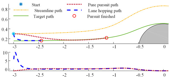
Figure 15.
The comparison of pure pursuit and lane hopping: path (upper plot) and curvature (lower plot). Horizontal axis is the forward +x direction.
5.2. Multi-Obstacles Environment
5.2.1. Comparison with Streamline Path by Weighting Velocity of Each Single Obstacle
In Figure 16, the proposed method is compared with the streamline path obtained via the weighting method. The maximum curvature of the pure pursuit path and streamline path are 0.50 (1/m) and 1.44 (1/m), respectively. The maximum curvature of the pure pursuit path is smaller than the streamline path.
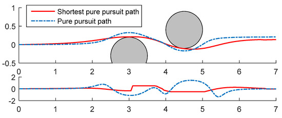
Figure 16.
The two obstacle environment. Comparison of the pure pursuit path and weighting streamline path.
5.2.2. Clutter Case: Comparison with Lau’s Approach
In this example, we compare our methods with a fluid motion planner provided by Lau et al. [18] in Figure 17. In the clutter case, there are two feasible paths with curvature constraints of 0.3 (1/m) and 0.8 (1/m), respectively, by our proposed method. On the other hand, the streamline path with curvature constraints 1 (1/m) collides with an obstacle and fails due to a late response. In sum, our proposed method performed well and can have a higher probability to get feasible paths with a small maximum curvature.
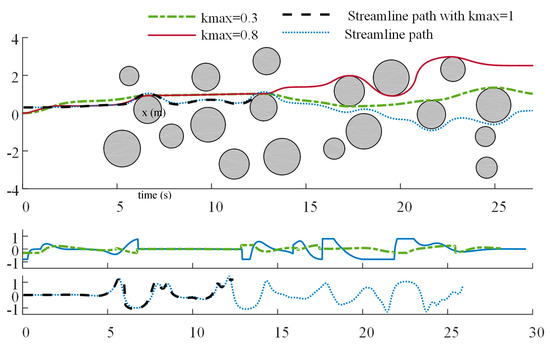
Figure 17.
A cluttered environment: upper plot = the paths, lower plots = the curvature. Black dashed path denotes the path generated by the method of superposition that collides with the obstacle.
5.3. Proof of Concept Experiment and Discussion
In the performed indoor experiment, three aspects related to the feasibility of trajectory generation are presented, which are (1) curvature constraint, (2) arrangement of obstacles, and (3) sensor detection error. First, while the maximum curvature constraint decreases, it is more difficult for robots to achieve primitive paths. Second, a robot needs to keep enough clearance from the obstacle to ensure the pursuit of all the three primitive paths possible. Third, we rely on low-cost sonar and infrared sensors to estimate the obstacle location. Furthermore, in order to guarantee obstacle avoidance, the obstacles are arranged so that only one obstacle is detected within a pre-specified look-ahead distance of the mobile robot’s current location at a time. Table 1 lists the parameters of the robot platform related to the experiment.

Table 1.
The parameters of the mobile robot Dr. Robot X80 (Figure 1) used for the experiment.
5.3.1. Experimental Setting
The robot and the obstacle are modeled as a circle defined by its radius rRobot = 0.2 m (Table 1), rObstacle = 0.1 m, respectively. The mobile robot is initially located at the origin of the global coordinate system and its initial forward moving direction is the + x-axis. The mobile robot is modeled as a kinematic unicycle (1) with curvature as a constrained input bounded by the maximum curvature (Figure 2) while the tangential speed is held constant with . The robot pose is obtained by numerically integrating Equation (1), which is directly controlled by the path curvature or angular velocity with the maximum allowable curvature for the mobile robot set as 1.5 (1/m), as shown in Table 1. Thus, the angular speed is upper bounded by The pure pursuit command rate is 10 Hz, and the safety distance is rSafe = 0.1 m, which is the robot displacement in a period to allow a sharp turn in case of an imminent collision. Given a safety distance rSafe between a robot and a detected obstacle, the radius of the obstacle is enlarged to account for the robot radius as rObs = rObstacle + rRobot + rSafe = 0.4 m for guaranteed local obstacle avoidance. In our experiment, the look-ahead distance is equal to the robot radius L = rRobot = 0.2 m. Note that if different subgoals between the obstacles are selected online for streamline changing from the current robot pose, we obtain topologically different paths with different curvatures for sequential obstacle avoidance in an environment with multiple obstacles. This is seen in the experiment in the following.
The distance between the robot’s center and the obstacle’s center is D = DSensor + rObstacle + rRobot, where DSensor is the range value measured by the sensor. In the case of a circular robot and a circular obstacle, which is the case studied in this paper, the collision-free criterion for safe navigation is that the distance D between the point robot (robot center) and the obstacle center is larger than rObs, i.e., D > 0.4. In the experiment reported here, a left/right turn is the default action and must maintain at least 0.4 m to a detected obstacle to be avoided. A narrow passage is not considered in this proof of concept experiment, since this default action may cause navigation difficulty, if not an impossibility in such a situation.
5.3.2. Online static cylinder obstacles avoidance
The experimental setup for the task of avoidance of multiple obstacles is operating a mobile robot Dr. Robot X80 in a cluttered indoor environment. Similar to Reference [11], there are four cylinder obstacles, all assumed to be identical cylinders with radius rObstacle = 0.1 m, placed at (1, 0), (1.8, −0.6), (2.6, 0) and (2.6, −1.2) in meters, which are distributed around the forward motion route. The velocity field generated by the gradient of the HPF solution to Laplace’s Equation for this map is depicted in Figure 18. We assume the following:
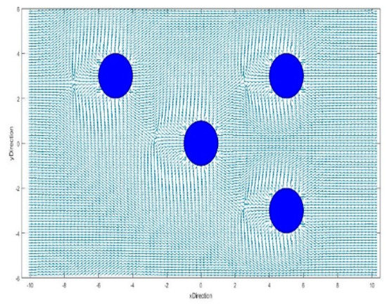
Figure 18.
The smooth velocity field generated by Laplace’s Equation with Dirichlet boundary conditions in the experiment scenario depicted in Figure 19, assuming a bounded rectangular domain with circular obstacles sufficiently apart.
- (i)
- We do not consider the navigation between very tight spaces, thus, the obstacles are arranged far apart to avoid the difficulty of APF-based navigation within a narrow passage. We arrange the clearance between any two adjacent obstacles smaller than the sensing range of the sensors but large enough to allow the pure pursuit algorithm to generate a local collision-free path for navigation. Specifically, the minimum distance between two obstacles’ centers is 2rObs = 0.8 m, wide enough for the robot to pass between two obstacles.
- (ii)
- The projection of all obstacles onto the ground plane is an identical circle, but the number of static obstacles and their locations are unknown.
The navigation trajectories generated in the experiment are depicted in Figure 19, along with Figure 20 showing the corresponding velocities and the path curvature profiles of two navigation paths with nearly the same starting point at the origin. The velocity field covers the free space and does not pass through the obstacles as desired. For the experiment shown here in Figure 19, the robot starts at the origin and initially follows a straight streamline trajectory with a speed of along the +x-axis. Then it confronts the detected obstacles in the front, and two feasible smooth navigation paths are generated for online safe and smooth navigation via the proposed HPF-based planner during the experiment. Different paths are obtained due to the slight variation in the initial position and heading of the mobile robot. It is noted that the portion of the two smooth paths is between two obstacles, thus no collision is guaranteed, and the maximum curvature of either path does not violate the maximum curvature. As remarked in Reference [28], the smoothness of the trajectory and its gradient is generic due to the physical characteristics of the continuously differentiable velocity potential solution to Laplace’s Equation mentioned in Section 3. The map of the environment is created by Hector SLAM, an open source SLAM algorithm available in ROS [23] based on the laser range data processed after the experiment. The robot can autonomously localize itself once new sensor readings are available (within 1 ms). The location of the detected obstacle fluctuates because of sensor noise and detection error. In this scenario, the primitive paths can be computed within 0.2 ms in our implementation. The obstacle avoidance system based on a priori selection of fast computing primitive streamline paths is computationally efficient, and the reaction time is able to handle the situation as obstacles in the front are detected, thus, making the system real-time. We remark that other options of a wide range of more involved trajectories such as B-spline [45] are applicable for the proposed obstacle avoidance system depicted in Figure 11, not only pertinent to streamlines. The main computational requirement is that the trajectories employed as primitive paths compatible with curvature constraint are a priori computed and could be online selected based on some rules, thus, preventing the generation of infeasible paths.
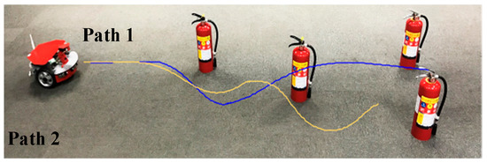
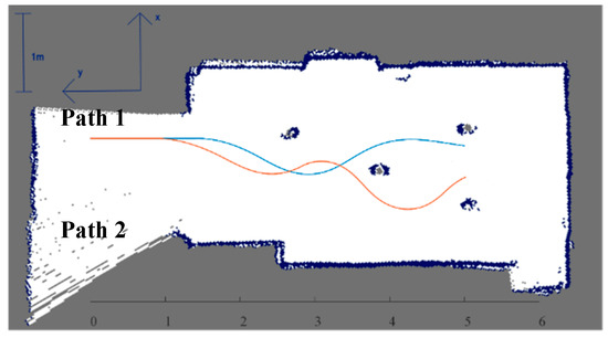
Figure 19.
The experimental setup for operating a mobile robot in a cluttered environment (upper: the photo, lower: the mapping) and two resulting obstacle-avoiding navigation paths generated online by the streamline-based approach.
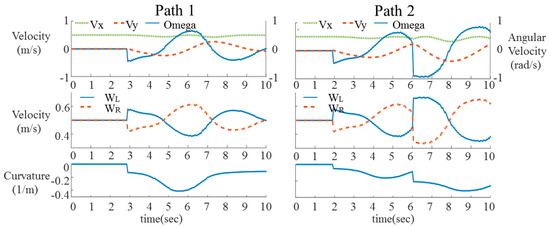
Figure 20.
The linear and angular velocities, speeds of the left and right wheels and curvature profiles of the two directional navigation paths depicted in Figure 19, where is the desired constant reference longitudinal/forward/tangential speed and is the lateral speed of the robot.
6. Conclusions
Recent developments on navigation methodologies for autonomous unmanned vehicles show that the HPF-based navigation algorithm is an example of the unifying view or framework of a vector field or dynamical systems based vehicle navigation pattern generators inspired from the scalar function of APFs (e.g., Reference [38]). The streamlines provide a pool of systematic, predictable smooth primitive paths that are integral curves of explicit and easily computable vector fields useful for the specification of the path tangent for directional navigation guidance and higher order path characteristics such as the curvature at each point of the path followed by autonomous vehicles. We demonstrate the practical usefulness of an HPF-based method to generate smooth paths for non-holonomic mobile robots to avoid obstacles via an obstacle avoidance system based on streamlines with a curvature constraint in this paper. First, streamlines extracted from the harmonic potential field are used to design three primitive smooth paths satisfying the curvature constraint for a single obstacle avoidance along with their application situations according to a lateral distance relative to obstacle size. Second, the pure pursuit algorithm is implemented to pursuit streamline-changing paths satisfying the curvature constraint for local multiple-obstacle avoidance situations. The simulation results show that pure pursuit paths in combination with initially planned streamlines can find feasible paths with smaller curvature constraints compared to previous hydrodynamics-based approaches. Furthermore, a proof of concept experiment was conducted to validate that the obstacle avoidance system based on the a priori selection of fast computing primitive streamline paths is computationally efficient and that the reaction time is able to handle the situation of an obstacle being detected in front of it online. Future work is planned to focus on the extension to 3D space, and toward safe navigation in environments of increasing size and complexity such as moving obstacles and multiple vehicles scenarios with the complete real-time HPF-based path planner. Additionally, it is also interesting to see the navigation performance under different sensor qualities such as the RGB-D sensor.
Author Contributions
P.-L.K. wrote the initial draft, P.-L.K. and C.-H.W. conducted the experiment, H.-J.C. worked on HPF simulation, J.-S.L. worked as PI of the whole project.
Funding
This research was funded by IIS, Academia Sinica.
Conflicts of Interest
The authors declare that there is no conflict of interest.
References
- Dong, J.F.; Sabastian, S.E.; Lim, T.M.; Li, Y.P. Autonomous In-door Vehicles. In Handbook of Manufacturing Engineering and Technology; Springer: London, UK, 2015. [Google Scholar]
- Adouane, L. Autonomous Vehicle Navigation: From Behavioral to Hybrid Multi-Controller Architectures; CRC Press: Boca Raton, FL, USA, 2016. [Google Scholar]
- Kunchev, V.; Jain, L.; Ivancevic, V.; Finn, A. Path planning and obstacle avoidance for autonomous mobile robots: A review. In Knowledge-Based Intelligent Information and Engineering Systems, Proceedings of the 10th International Conference, KES 2006, Bournemouth, UK, 9–11 October 2006; Springer: Berlin, Germany, 2006; pp. 537–544. [Google Scholar]
- Minguez, J.; Lamiraux, F.; Laumond, J.-P. Motion planning and obstacle avoidance. In Handbook of Robotics; Springer: Basel, Switzerland, 2016; pp. 1177–1202. [Google Scholar]
- Khatib, O. Real-time obstacle avoidance for manipulators and mobile robots. In Proceedings of the IEEE International Conference on Robotics and Automation, St. Louis, MO, USA, 25–28 March 1985; pp. 500–505. [Google Scholar]
- Fahimi, F. Obstacle avoidance using harmonic potential functions. In Autonomous Robots; Springer: Boston, MA, USA, 2009; pp. 1–49. [Google Scholar]
- Connolly, C.I.; Grupen, R.A. On the applications of harmonicfunctionsto robotics. J. Robot. Syst. 1993, 10, 931–946. [Google Scholar] [CrossRef]
- Kaľavský, M.; Ferková, Ž. Harmonic potential field method for path planning of mobile robot. ICTIC 2012, 1, 41–46. [Google Scholar]
- Akishita, S.; Kawamura, S.; Hayashi, K. New navigation function utilizing hydrodynamic potential for mobile robot. In Proceedings of the IEEE International Workshop on Intelligent Motion Control, Istanbul, Turkey, 20–22 August 1990; pp. 413–417. [Google Scholar]
- Wray, K.H.; Ruiken, D.; Grupen, R.A.; Zilberstein, S. Log-space harmonic function path planning. In Proceedings of the IEEE/RSJ International Conference onIntelligent Robots and Systems, Daejeon, Korea, 9–14 October 2016; pp. 1511–1516. [Google Scholar]
- Waydo, S.; Murray, R.M. Vehicle motion planning using stream functions. In Proceedings of the IEEE International Conference on Robotics and Automation, Taipei, Taiwan, 14–19 September 2003; pp. 2484–2491. [Google Scholar]
- Daily, R.; Bevly, D.M. Harmonic potential field path planning for high speed vehicles. In Proceedings of the American Control Conference, Seattle, WA, USA, 11–13 June 2008; pp. 4609–4614. [Google Scholar]
- Owen, T.; Hillier, R.; Lau, D. Smooth path planning around elliptical obstacles using potential flow for non-holonomic robots. In Robot Soccer World Cup; Springer: Berlin/Heidelberg, Germnay, 2011; pp. 329–340. [Google Scholar]
- Palm, R.; Driankov, D. Fluid mechanics for path planning and obstacle avoidance of mobile robots. In Proceedings of the 11th International Conference on Informatics in Control, Automation and Robotics (ICINCO), Vienna, Austria, 1–3 September 2014; pp. 231–238. [Google Scholar]
- Kim, J.O.; Khosla, P. Real-time obstacle avoidance using harmonic potential functions. In Proceedings of the IEEE International Conference on Robotics and Automation, Sacramento, CA, USA, 9–11 April 1991; pp. 790–796. [Google Scholar]
- Wang, H.; Lyu, W.; Yao, P.; Liang, X.; Liu, C. Three-dimensional path planning for unmanned aerial vehicle based on interfered fluid dynamical system. Chin. J. Aeronaut. 2015, 28, 229–239. [Google Scholar] [CrossRef]
- Connolly, C.I.; Grupen, R.A. Nonholonomic Path Planning Using Harmonic Functions; National Science Foundation: Alexandria, VA, USA, 1994.
- Lau, D.; Eden, J.; Oetomo, D. Fluid Motion Planner for Nonholonomic 3-D Mobile Robots with Kinematic Constraints. IEEE Trans. Robot. 2015, 31, 1537–1547. [Google Scholar] [CrossRef]
- Munson, B.R.; Young, D.F.; Okiishi, T.H. Fundamentals of Fluid Mechanics; Fowley, D., Ed.; John Wiley & Sons, Inc.: New York, NY, USA, 1990. [Google Scholar]
- Coulter, R.C. Implementation of the Pure Pursuit Path Tracking Algorithm; DTIC Document; Defense Technical Information Center: Fort Belvoir, WV, USA, 1992. [Google Scholar]
- Morales, J.; Martínez, J.L.; Martínez, M.A.; Mandow, A. Pure-pursuit reactive path tracking for nonholonomic mobile robots with a 2D laser scanner. EURASIP J. Adv. Signal Process. 2009, 2009, 935237. [Google Scholar] [CrossRef]
- Masoud, A.A. Kinodynamic motion planning. IEEE Robot. Autom. Mag. 2010, 17, 85–99. [Google Scholar] [CrossRef]
- Kohlbrecher, S.; von Stryk, O.; Meyer, J.; Klingauf, U. A flexible and scalable slam system with full 3d motion estimation. In Proceedings of the IEEE International Symposium on Safety, Security, and Rescue Robotics, Kyoto, Japan, 1–5 November 2011. [Google Scholar]
- Belabbas, M.A.; Liu, S. New method for motion planning for non-holonomic systems using partial differential equations. In Proceedings of the American Control Conference, Seattle, WA, USA, 24–26 May 2017; pp. 4189–4194. [Google Scholar]
- Gingras, D.; Dupuis, E.; Payre, G.; de Lafontaine, J. Path planning based on fluid mechanics for mobile robots using unstructured terrain models. In Proceedings of the IEEE International Conference on Robotics and Automation, Anchorage, AK, USA, 3–7 May 2010; pp. 1978–1984. [Google Scholar]
- Motonaka, K. Kinodynamic Motion Planning for a Two-Wheel-Drive Mobile Robot. In Handbook of Research on Biomimetics and Biomedical Robotics; IGI Global: Hershey, PA, USA, 2018; pp. 332–346. [Google Scholar]
- Liu, C.A.; Wei, Z.; Liu, C. A new algorithm for mobile robot obstacle avoidance based on hydrodynamics. In Proceedings of the IEEE International Conference on Automation and Logistics, Jinan, China, 18–21 August 2007; pp. 2310–2313. [Google Scholar]
- Golan, Y.; Edelman, S.; Shapiro, A.; Rimon, E. Online Robot Navigation Using Continuously Updated Artificial Temperature Gradients. IEEE Robot. Autom. Lett. 2017, 2, 1280–1287. [Google Scholar] [CrossRef]
- Louste, C.; Liégeois, A. Path planning for non-holonomic vehicles: a potential viscous fluid field method. Robotica 2002, 20, 291–298. [Google Scholar] [CrossRef]
- Pedersen, M.D.; Fossen, T.I. Marine vessel path planning & guidance using potential flow. IFAC Proc. Vol. 2012, 45, 188–193. [Google Scholar]
- LaValle, S.M. Planning Algorithms; Cambridge University Press: New York, NY, USA, 2006. [Google Scholar]
- Tanner, H.G.; Loizou, S.; Kyriakopoulos, K.J. Nonholonomic stabilization with collision avoidance for mobile robots. In Proceedings of the IEEE/RSJ International Conference on Intelligent Robots and Systems, Maui, HI, USA, 29 October–3 November 2001; pp. 1220–1225. [Google Scholar]
- Galick, M. The planning of optimal motions of non-holonomic systems. Nonlinear Dyn. 2017, 90, 2163–2184. [Google Scholar] [CrossRef]
- Li, L. Nonholonomic motion planning using trigonometric switch inputs. Int. J. Simul. Model. (IJSIMM) 2017, 16, 176–186. [Google Scholar] [CrossRef]
- Lamiraux, F.; Bonnafous, D. Reactive trajectory deformation for nonholonomic systems: Application to mobile robots. In Proceedings of the IEEE International Conference on Robotics and Automation, Washington, DC, USA, 11–15 May 2002; pp. 3099–3104. [Google Scholar]
- Kelly, A.; Nagy, B. Reactive nonholonomic trajectory generation via parametric optimal control. Int. J. Robot. Res. 2003, 22, 583–601. [Google Scholar] [CrossRef]
- Ho, Y.-J.; Liu, J.-S. Collision-free curvature-bounded smooth path planning using composite Bezier curve based on Voronoi diagram. In Proceedings of the IEEE International Symposium on Computational Intelligence in Robotics and Automation, Daejeon, Korea, 15–18 December 2009; pp. 463–468. [Google Scholar]
- Panagou, D. Motion planning and collision avoidance using navigation vector fields. In Proceedings of the IEEE International Conference on Robotics and Automation, Hong Kong, China, 31 May–7 June 2014; pp. 2513–2518. [Google Scholar]
- Papoutsidakis, M.; Piromalis, D.; Neri, F.; Camilleri, M. Intelligent algorithms based on data processing for modular robotic vehicles control. WSEAS Trans. Syst. 2014, 13, 242–251. [Google Scholar]
- Bekey, G.A. Autonomous Robots: From Biological Inspiration to Implementation and Control; MIT Press: Cambridge, MA, USA 2005. [Google Scholar]
- Lo, C.-W.; Wu, K.-L.; Lin, Y.-C.; Liu, J.-S. An intelligent control system for mobile robot navigation tasks in surveillance. In Robot Intelligence Technology and Applications 2; Springer: Berlin, Germany, 2014; pp. 449–462. [Google Scholar]
- Schoof, E.; Manzie, C.; Shames, I.; Chapman, A.; Oetomo, D. An experimental platform for heterogeneous multi-vehicle missions. In Proceedings of the International Conference on Science and Innovation for Land Power, Adelaide, Australia, 5–6 September 2018. [Google Scholar]
- Giftthaler, M.; Sandy, T.; Dörfler, K.; Brooks, I.; Buckingham, M.; Rey, G.; Kohler, M.; Gramazio, F.; Buchli, J. Mobile robotic fabrication at 1:1 scale: The in situ fabricator. Constr. Robot. 2017, 1, 3–14. [Google Scholar] [CrossRef]
- Rösmann, C.; Hoffmann, F.; Bertram, T. Integrated online trajectory planning and optimization in distinctive topologies. Robot. Auton. Syst. 2017, 88, 142–153. [Google Scholar] [CrossRef]
- Kano, H.; Fujioka, H. B-Spline Trajectory Planning with Curvature Constraint. In Proceedings of the Annual American Control Conference, Milwaukee, WI, USA, 27–29 June 2018; pp. 1963–1968. [Google Scholar]
© 2018 by the authors. Licensee MDPI, Basel, Switzerland. This article is an open access article distributed under the terms and conditions of the Creative Commons Attribution (CC BY) license (http://creativecommons.org/licenses/by/4.0/).