Article

Improving Bearing Fault Diagnosis Using Maximum Information Coefficient Based Feature Selection

1
Key Laboratory of Advanced Manufacturing Technology, Ministry of Education, Guizhou University, Guiyang 550025, China
2
State Key Laboratory of Public Big Data, Guizhou University, Guiyang 550025, China
3
State Key Laboratory of Digital Manufacturing Equipment and Technology, Huazhong University of Science and Technology, Wuhan 430074, China
4
School of Mechanical Engineering, Guizhou University, Guiyang 550025, China
*
Authors to whom correspondence should be addressed.
Appl. Sci. 2018, 8(11), 2143; https://doi.org/10.3390/app8112143
Submission received: 8 October 2018 / Revised: 26 October 2018 / Accepted: 30 October 2018 / Published: 2 November 2018
(This article belongs to the Special Issue Fault Detection and Diagnosis in Mechatronics Systems)

Abstract

:
Effective feature selection can help improve the classification performance in bearing fault diagnosis. This paper proposes a novel feature selection method based on bearing fault diagnosis called Feature-to-Feature and Feature-to-Category- Maximum Information Coefficient (FF-FC-MIC), which considers the relevance among features and relevance between features and fault categories by exploiting the nonlinearity capturing capability of maximum information coefficient. In this method, a weak correlation feature subset obtained by a Feature-to-Feature-Maximum Information Coefficient (FF-MIC) matrix and a strong correlation feature subset obtained by a Feature-to-Category-Maximum Information Coefficient (FC-MIC) matrix are merged into a final diagnostic feature set by an intersection operation. To evaluate the proposed FF-FC-MIC method, vibration data collected from two bearing fault experiment platforms (CWRU dataset and CUT-2 dataset) were employed. Experimental results showed that accuracy of FF-FC-MIC can achieve 97.50%, and 98.75% on the CWRU dataset at the motor speeds of 1750 rpm, and 1772 rpm, respectively, and reach 91.75%, 94.69%, and 99.07% on CUT-2 dataset at the motor speeds of 2000 rpm, 2500 rpm, 3000 rpm, respectively. A significant improvement of FF-FC-MIC has been confirmed, since the p-values between FF-FC-MIC and the other methods are 1.166 × 10 3 , 2.509 × 10 5 , and 3.576 × 10 2 , respectively. Through comparison with other methods, FF-FC-MIC not only exceeds each of the baseline feature selection method in diagnosis accuracy, but also reduces the number of features.

1. Introduction

As one of the most significant parts of rotating machines, rolling bearing has a great influence on operating status of mechanical equipment. According to the statistics of mechanical faults, more than 40% of the faults are caused by rolling bearings [1,2]. Therefore, it is important and meaningful for researchers to do research on fault diagnosis of rolling bearings. In bearing fault diagnosis, an essential role to improve the diagnosis accuracy of bearings is played by feature selection, which aims at selecting a subset from the original set of features according to discrimination capability [3].
Traditional feature selection methods can be divided into three types: filters, wrappers and embedded methods [4]. Filter methods evaluate the quality of features through some feature evaluation criteria and select the top high-ranked features. Based on the advantages of high generality and low computational cost, filter-based feature selection methods are suitable for high-dimensional datasets [5,6]. Although filter-based methods are computationally fast, they usually do not take feature relevance into considerations. Wrapper methods utilize the performance of machine learning model to judge the quality of the feature subset. They usually repeat the two steps, including searching for an optimal feature subset and evaluating the selected features, until a stopping measure is met [5,6]. The computational speed of wrapper-based methods is slow and the computational complexity is high, because of search strategies which involve sequential selection algorithms like sequential forward selection (SFS), sequential backward selection (SBS) and heuristic search algorithms like genetic algorithms (GAs), particle swarm optimization (PSO), gravitational search algorithm (GSA), and ant colony optimization (ACO). The complementary strengths of both filter and wrapper are exploited by embedded methods. Embedded methods define the feature that has the best ability to differentiate among classes in each stage and take feature selection as part of the training process. Thus, embedded methods are more effective than filter approaches since they involve interaction with the learning algorithm, and they are superior to wrapper methods as they do not need to evaluate the feature subsets iteratively [5]. However, embedded methods have the shortcomings of low computational speed and high computational complexity as well.
As mentioned above, feature selection in bearing fault diagnosis is helpful to improve the accuracy of diagnosis and reduce the dimensions of features. Fu [7] combined filter and wrapper methods to select features in bearing fault diagnosis. Ou [8,9] proposed a supervised Laplacian score (SLS)-based feature selection method. Hui [10] applied an improved wrapper-based feature selection method for bearing fault diagnosis. Liu [11] selected features through an evolutionary Monte Carlo method, which is a wrapper-based method. Islam [12] proposed a hybrid feature selection method which employed a genetic algorithm (GA)-based filter analysis to select optimal features. Luo [13] used the real-valued gravitational search algorithm (RGSA) to optimize the input weights and bias of extreme learning machine (ELM), and the binary GSA (BGSA) was used to select important features from a compound feature set. Yu [14] combined the K-means method with standard deviation to select the most sensitive characteristics. Liu [15] and Yang [16] utilized distance evaluation technique (DET) to select sensitive features. Vepa [17] presented a feature selection method involved in feature weight, monotonicity, correlation, and robustness. However, the above methods have some problems that lack considerations for relevance; for example, the computational speed is slow, and the computational complexity is high.
Some researchers recently took signal relevance into consideration. Cui [18] selected intrinsic mode functions (IMFs) as features through correlation. A correlation coefficient of two simplified neutrosophic sets (SNSs) was proposed to diagnose the bearing fault types by Shi [19]. In [20], Laplacian Score (LS) for feature selection was utilized to refine the feature vector by sorting the features according to their importance and correlations. Besides, Zhang [21] employed the Decision Tree algorithm to select the important features of the time-domain signal, and the low correlation features was selected. Jiang [22] computed the mutual information (MI) of decomposed components and the original signal, and extracted the noiseless component, in order to obtain the reconstructed signal. However, in terms of relevance, researchers did not take relevance between features and fault categories into account in feature selection, only considering the correlation between features.
The purpose of feature selection is not just simply reducing dimensions for the data. It is more about eliminating redundant and irrelevant features. Redundant features can be eliminated by the measurement of relevance among features. The stronger the relevance between two features, the stronger the redundancy and replaceability between them. Moreover, irrelevant features can be eliminated through the measurement of relevance between features and categories. The stronger the relevance between features and categories, the stronger the distinguishability of features from categories. Irrelevant and redundant features can be eliminated from a raw feature set according to relevance. Therefore, consideration of relevance plays an essential role in reducing data dimensions in feature selection.
On the other hand, some work [8,9,10,11,12,13] selected features based on wrapper methods and increased the computational complexity. To avoid the cost of searching, the idea of intersection or union operation was put forward to merge feature subsets [23,24].
When it comes to the problem of coping with redundant information, principal component analysis (PCA) has been extensively studied. PCA is an algorithm that can effectively extract subsets from data by reducing the dimensions of the data set [25]. Since the principal component includes most information of the raw features which are irrelevant and do not contain redundant information, the principal component can be used to replace raw features. Based on this, PCA can realize data reduction and reduce the complexity of data processing, preventing dimensional disaster [26]. Typical PCA algorithms like those in [27,28,29,30] are used to extract features and to reduce data dimensions.
Based on the problems mentioned above, a novel feature selection method called FF-FC-MIC based on the Feature-to-Category-Maximum Information Coefficient is proposed. The main contributions of this paper are as follows:
(1)
A new frame of feature selection is proposed for bearing fault diagnosis, which aims at considering the relevance among features and the relevance between features and fault categories. In the new feature selection frame, strong relevance features are eliminated by an FF-MIC matrix based on the relevance between features and features. On the contrary, strong relevance features are selected by the FC-MIC matrix based on the relevance between features and categories. The proposed frame can eliminate not only redundant features but also irrelevant features from the feature set.
(2)
In order to avoid computational complexity brought by wrapper methods, an intersection operation is applied to merge the obtained feature subsets. The intersection operation has advantages of forming a final subset with a lower dimension and saving time, instead of subset searching.
(3)
This paper applied two datasets to validate the effectiveness and adaptability of proposed method. It turned out the proposed method has a good applicability and stability.
The remainder of this paper is organized as follows. Section 2 introduces the basic theory and algorithm applied in this paper. Section 3 gives the details of the proposed method. Section 4 shows the experimental results. Section 5 concludes the findings shown in this paper.

2. Related Basic Theory and Algorithm

Based on the two main problems mentioned before, relevance and computational complexity, the related theory for solving the problems are listed in this section. First, the maximum information coefficient (MIC) is used to measure the relevance between features and features, and the relevance between features and categories. Second, an intersection operation is employed so that it can avoid high computational complexity. Third, in order to reduce data dimensions for further and to shorten the training time of classification model, the PCA algorithm is utilized.

2.1. Maximum Information Coefficient

The MIC cannot only measure linear relationships and nonlinear relationships, but can extensively excavate non-functional dependencies between variables. MIC mainly works with MI and meshing methods. MI is an indicator of the degree of correlation between variables. Given a variable A = { a i , i = 1 , 2 , , n } and B = { b i , i = 1 , 2 , , n } , where n is the number of samples, the MI is defined as follow:
  MI ( A , B ) = a A b B p ( A , B ) l o g 2 p ( A , B ) p ( A ) p ( B )  
where p ( A , B ) is the joint probability density of A and B, and p ( A )   and   p ( B ) are the boundary probability densities of A and B, respectively. Suppose D = { ( a i , b i ) , i = 1 , 2 , , n } is a set of finite ordered pairs. It defines a division G , dividing the value range of variable   A into x segments and also dividing the value range of variable B into y segments. Therefore, the G is a grid with a size of x × y . Meanwhile, MI ( A , B ) in each grid is calculated. Since the same grid with a size of x × y has several ways of dividing, the maximum value of MI ( A , B ) in different ways of dividing is chosen as the MI value of a division G . Additionally, a definition of maximum MI under a division G is as follow:
  MI * ( D , x , y ) = m a x MI ( D | G )  
where D | G denotes data D are divided by G . Although it utilizes MI to indicate the quality of the grid, MIC is not just simply estimating the MI. A characteristic matrix is formed by maximum normalized MI values under different divisions. The characteristic matrix is defined as follow:
  MI ( D ) x , y = MI * ( D , x , y ) l o g m i n { x , y }  
Moreover, the MIC is defined as:
  MIC ( D ) = max x y < B ( n ) { MI ( D ) x , y }  
where B ( n )   is the upper limit of the x × y   grid. Generally, ω ( 1 ) < B ( n ) < O ( n 1 ε ) , where 0 < ε < 1 .

2.2. Merging Feature Subsets

Merging feature subsets usually has two ways. One is the intersection approach and the other is the union approach.
Let S be the set of samples and F = { f 1 , f 2 , , f i } be the feature set after preprocessing. F S 1 = { f 1 , f 2 , , f m } is a subset of features selected with filter ( M 1 ), where m denotes the number of features which are selected by M 1 and m < i .   F S 2 = { f 1 , f 2 , , f n } is a subset of features selected with filter ( M 2 ), where n denotes the number of features which are selected by M 2 and n < i .
The union approach is to create a feature subset F S 3 , which has the number of features p   ( p { m , n } ) , by merging all features in F S 1 and in F S 2 :
  F S 3 = F S 1 F S 2  
The intersection approach is to create a feature subset F S 4 , which has the number of features q ( q { m , n } ) , including these features that are present in both feature subsets F S 1   and   F S 2 .
  F S 4 = F S 1 F S 2  
Usually, the two approaches mentioned above are utilized to merge feature subsets selected by different filter-based feature selection methods. The union approach selects all features in both subsets. At the same time, it increases the number of features and does not achieve the goal of reducing data dimensions. On the contrast, the intersection approach selects only common features. It reduces the total number of features. However, it is possible to lose some features which are proficient [31].

3. Proposed Method

A new feature selection method was proposed to address two issues in feature selection: relevance and computational complexity.
The MIC cannot only measure the relevance between features and features, but also measure the relevance between features and categories. The method is divided into two parallel steps to select features from both aspects mentioned above. First, strong irrelevance features can be selected based on the MIC between features and features. Second, strong relevance features can be selected based on the MIC between features and fault categories. This frame has the advantage of a comprehensive consideration of relevance to eliminate redundant and irrelevant features from a feature set.
In term of computational complexity, an intersection operation is employed to merge feature subsets which are selected by the relevance between features and features, and by the relevance between features and fault categories. The intersection operation has the advantage of obtaining a lower-dimension final subset with a lower computational complexity, containing as much as information.
Based on the above consideration, MIC is applied to measure the relevance among features and the relevance between features and fault categories. In addition, to avoid computational complexity caused by wrapper methods, an intersection operation is applied, instead of wrapper methods, to merge subsets.
The detailed implementation steps are as follows. First, MIC among features and MIC between features and fault categories are calculated to obtain two MIC matrixes. MIC among features is called FF-MIC and MIC between features and categories is named FC-MIC. Second, strong relevance values in FF-MIC and in FC-MIC are calculated to distinguish strong and weak relevance features. Third, strong irrelevance features selected by FF-MIC and strong relevance features selected by FC-MIC are merged through an intersection operation to form a final feature subset. Finally, PCA is applied to further reduce dimensions of the final feature set. The whole process of feature selection is shown in Figure 1.

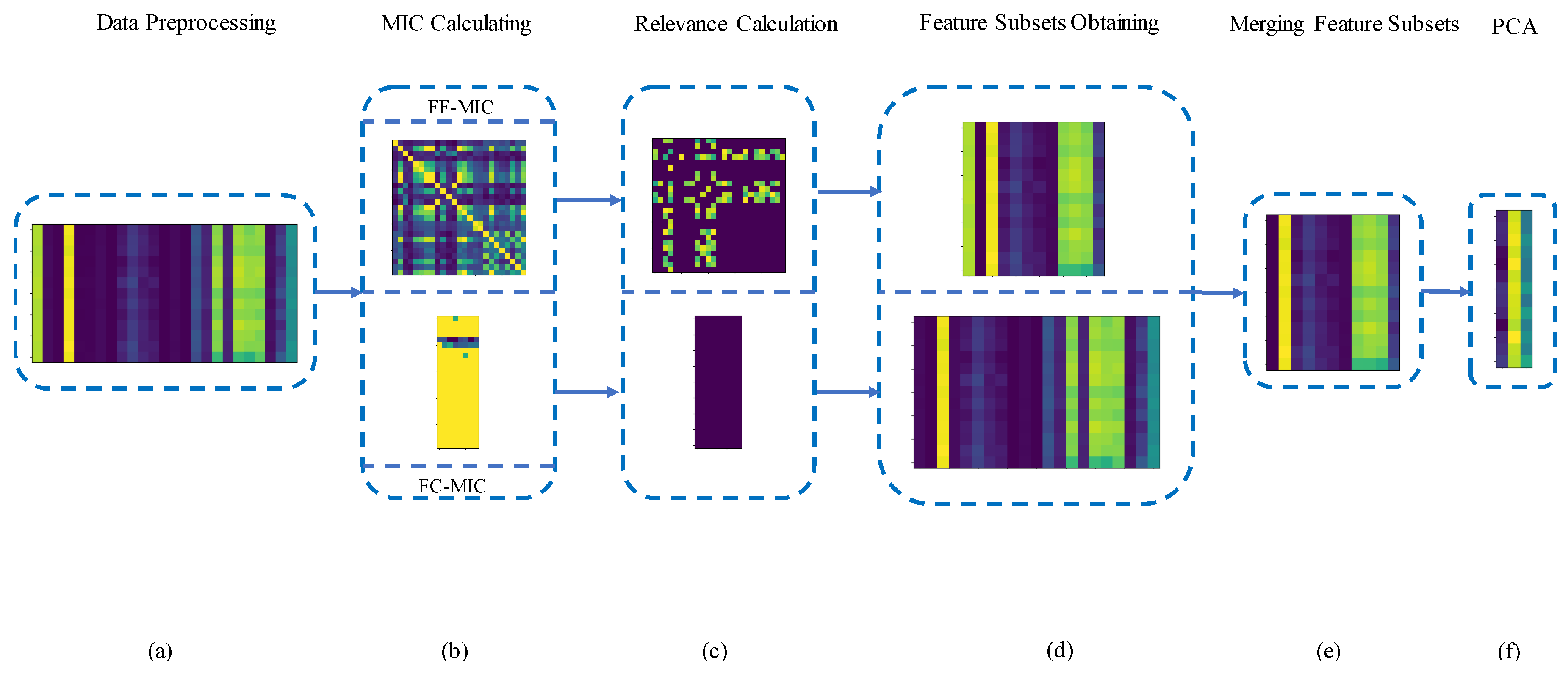
3.1. Data Preprocessing

Since the vibration signal measured by sensors carries vital information, it should be transformed by the appropriate action and sensitive features, which can efficiently reflect the bearing working condition will be obtained. To avoid missing sensitive features, almost all features in the time and frequency domains are acquired. In order to improve the convergence speed of the model and the accuracy of the model, all features will be performed by feature scaling after the features are obtained. The details are given in Algorithm 1.
Algorithm 1. Data preprocessing.
Input: samples: S = { s 1 , s 2 , s n } , where   n is the number of samples.
Output: the preprocessed feature set F S .
  • for each s i in S
  • calculate each feature value from both the time domain and frequency domain and scale each feature value to [0,1], forming a feature set: F S = { f 1 , f 2 , f m } , where m is the number of features
  • end for

3.2. MIC Calculation

MIC is used to define the relevance between features and features, and the relevance between features and categories. A matrix called FF-MIC is formed by the MIC between features and features, and a matrix called FC-MIC is formed by the MIC between features and fault categories. The construction details of FF-MIC and FC-MIC are described in Algorithm 2.
Algorithm 2. MIC calculation.
Input: F S = { f 1 , f 2 , f m } , where C = { c 1 , c 2 , c p }   are fault categories, and p is the number of fault categories.
Output: FF-MIC and FC-MIC.
  • for each f i , f j ( 1 i , j m ) in F S
  • calculate MIC between f i and f j , obtaining the FF-MIC matrix with a size of m × m ; the row and column denote the serial number of features.
  • for each f i in F S
  • for each c j in C
  • calculate MIC between f i and c j , obtaining the FC-MIC matrix with a size of m × p ; the row denotes the serial number of features and the column denotes the serial number of fault categories.
  • end for

3.3. Relevance Calculation

As mentioned before, the value of MIC ranges from 0 to 1. FF-MIC denotes a matrix which can measure the relevance between features and features. The closer to 0 each element in the FF-MIC matrix approaches, the stronger the irrelevance between the features corresponding to the row and column of the element is. On the contrary, the closer to 1 each element in the FC-MIC matrix approaches, the stronger the relevance between the feature and category is. On this basis, a feature can be judged whether it is a weak relevance or strong relevance through the value in the FF-MIC matrix.
In each column of the FF-MIC matrix, each minimum value is found to form a set F F m i n = { m i n 1 ,   m i n 2 , , m i n m } , and then the maximum value   F F _ t h r e s h o l d is found in the set F F m i n . Therefore, the features, of which corresponding FF-MIC values are smaller than F F _ t h r e s h o l d are, are called strong irrelevance features. The reason of setting up F F m i n is that the condition of the strong irrelevance between a certain feature and each one in the rest can be observed. Through the set F F m i n , the maximum of F F m i n is utilized to judge whether a feature is strong irrelevant with other features.
At the same time, in each row of FC-MIC, each maximum value is found to form a set F C m a x = { m a x 1 ,   m a x 2 , , m a x m } , and then the minimum value   F C _ t h r e s h o l d is found in the set F F m a x . The features, of which corresponding FC-MIC values are bigger than the F C _ t h r e s h o l d , are called strong relevance features, which are being selected soon. The reason of setting up F C m a x is that the condition of the strongest relevance between a certain feature and each category can be observed. Through the set F C m a x , the minimum of F C m a x is utilized to judge whether a feature is strong relevant with categories.
The details of relevance calculation are shown in Algorithm 3.
Algorithm 3. Relevance calculation
Input: F S = { f 1 , f 2 , f m } , FF-MIC, and FC-MIC.
Output: F F _ t h r e s h o l d , and   F C _ t h r e s h o l d .
  • for each column in the FF-MIC matrix
  • for elements in each column
  • find each minimum value to form a set F F m i n = { m i n 1 ,   m i n 2 , , m i n m }
  • end for
  • for each m i n i in F F m i n
  • find the maximum F F _ t h r e s h o l d in F F m i n
  • end for
  • for each row in FC-MIC
  • for elements in each row
  • find each maximum value to form a set F C m a x = { m a x 1 ,   m a x 2 , , m a x m }
  • end for
  • for each m a x i in F C m i n
  • find the minimum F C _ t h r e s h o l d in F C m a x
  • end for

3.4. Obtaining Feature Subsets

After relevance calculation, two feature sets are formed called S u b s e t 1 and S u b s e t 2 , respectively, according to the F F _ t h r e s h o l d and   F C _ t h r e s h o l d . The features, of which corresponding FF-MIC values are smaller than the F F _ t h r e s h o l d , will be the elements of S u b s e t 1 , because the closer to 0 the FF-MIC value, the stronger the irrelevance between features. Additionally, the features, of which corresponding FC-MIC values are bigger than the F C _ t h r e s h o l d , will become the members of S u b s e t 2 , because the closer to 1 the FC-MIC value, the stronger the relevance between features and categories. The details of obtaining feature subsets are shown in Algorithm 4.
Algorithm 4. Obtaining feature subsets
Input: F S = { f 1 , f 2 , f m } , F F _ t h r e s h o l d , and   F C _ t h r e s h o l d .
Output: S u b s e t 1 and S u b s e t 2 .
  • for each f i in F S
  • select the features corresponding FF-MIC values smaller than the F F _ t h r e s h o l d to form a S u b s e t 1
  • end for
  • for each f i in F S
  • select the features corresponding FC-MIC values bigger than the F F _ t h r e s h o l d to form a S u b s e t 2
  • end for

3.5. Merging Feature Subsets and Reducing Dimensions with PCA

In above steps, two feature subsets are obtained. S u b s e t 1 is a strong-irrelevance subset which contains features with strong irrelevance among them. S u b s e t 2 is a strong-relevance subset which consists of features which have strong correlation with fault categories. First, an intersection operation is carried between S u b s e t 1 and S u b s e t 2 to obtain a final subset F S u b s e t .   F S u b s e t contains the common elements of S u b s e t 1 and S u b s e t 2 . Next, the variance of each feature is calculated and then the five features with the largest variance are selected. The reason of selecting the features with the five largest variances is that the smaller a variance of the feature, the less information this feature contains. Therefore, the five features with the largest variance means that almost all information is retained. Finally, PCA is employed to reduce dimensions of the F S u b s e t . The details are given in Algorithm 5.
Algorithm 5. Merging feature subsets.
Input: S u b s e t 1 and S u b s e t 2 .
Output: F S u b s e t .
  • Merge S u b s e t 1 and S u b s e t 2 with an intersection operation to obtain F S u b s e t .
  • for each f i in F S u b s e t
  • employ PCA to select five features with the largest variance
  • end for

4. Experimental Results and Analysis

In this paper, the proposed method was applied to two datasets. One was the vibration dataset provided by the Bearing Data Center of Case Western Reserve University (CWRU) [32], and the other was the vibration dataset which was obtained by the CUT-2 platform. Based on both datasets, the proposed method was compared with 3 traditional feature selection methods, which are filter based on variance, wrapper based on recursive feature elimination (RFE), and embedded based on gradient boosting decision tree (GBDT). Performances of these methods were evaluated by the diagnosis accuracy on two popular fault classification models, which are Support Vector Machine (SVM) and K-Nearest Neighbor (KNN).
The features were calculated both in the time domain and frequency domain. All the features are shown in Table 1.

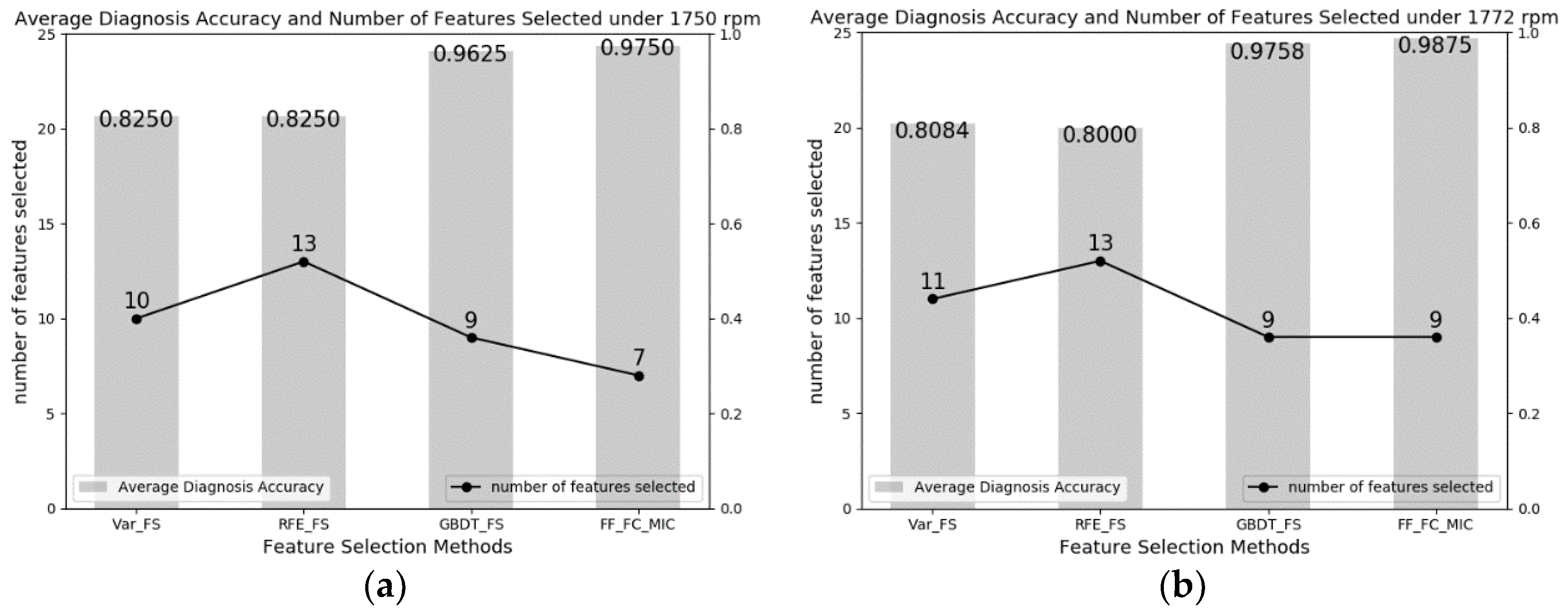
4.1. Experiments on CWRU Datasets

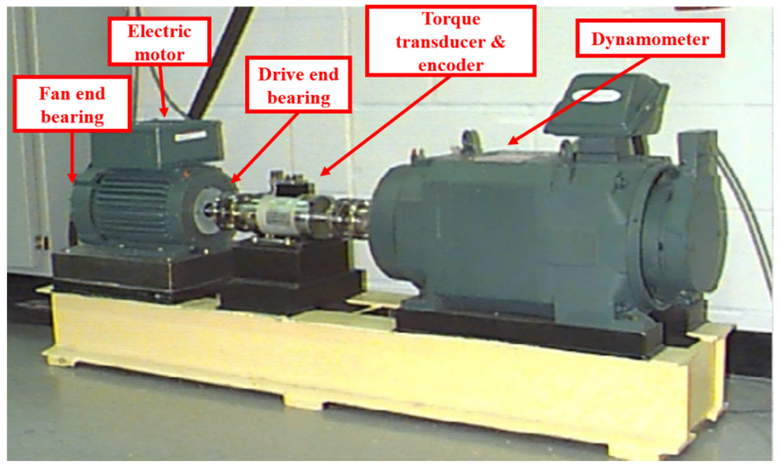
4.1.1. Experimental Setup and Datasets

Our datasets were constructed on CWRU bearing datasets [32] to apply the proposed method. As shown in Figure 2, the experimental test rig included an electric motor (left), a torque transducer/encoder (center), a dynamometer (right), and a control circuitry (not shown). The deep groove ball bearings of the type 6205-2RS JEM SKF at the drive end (DE) was used for vibration signal collection. The vibration signals were collected by accelerometers at 4 different motor speeds of 1797 rpm, 1772 rpm, 1750 rpm and 1730 rpm, where the sampling frequencies were 12 kHz and 48 kHz. The faults were set by an electric discharge machine with diameters of 0.007 inches, 0.014 inches, 0.021 inches and 0.028 inches.
There were 4 bearing categories, including 3 fault categories and 1 normal category. One hundred fifty samples were acquired in each category and each sample contains 1024 continuous data points. Two same datasets were constructed at the motor speeds of 1750 rpm and 1772 rpm. Table 2 shows the details of the datasets. The training process and the test process were carried out at the same speed. The training set included 420 samples and the testing set included 180 samples.

4.1.2. Result Analysis of CWRU Datasets

According to the proposed feature selection method, features selected by the proposed method are shown in Table 3.
As is shown in Table 3, at the motor speed of 1750 rpm, the proposed method selected 7 features from 25 features in total, and selected 9 features at the speed of 1772 rpm.
KNN and SVM classifiers and 3 traditional feature selection methods were applied to validate the proposed method. As mentioned before, 2 datasets were constructed at 1750 rpm and 1772 rpm. Both of them were used in the training and testing processes. The results are shown in Table 4.
As shown in Table 4, the proposed method has a higher accuracy than the other 3 feature selection methods. Especially, the best classification accuracy has achieved 100% at the motor speed of 1772 rpm with KNN. Comparing with the other 3 methods, the proposed method can improve the accuracy by about an average of 1.21% at least, and by about an average of 15.25% at most. Meanwhile, the classification accuracies of the proposed method at different motor speeds with 2 classifiers reached are all above 95%. Above all, it is obvious that the proposed method has a pretty performance on the aspect of diagnosis accuracy.
In addition, in order to validate the propose method’s effectiveness, the number of features selected is compared between the proposed method and the other 3 traditional methods. All the numbers of features selected by these 4 methods are shown in Figure 3.
In Figure 3, the number of features selected by the proposed method under both motor speeds is the minimum, comparing to those in the other 3 methods. In other words, the proposed method achieves a higher diagnosis accuracy based on fewer features. Fewer features indicate lower data dimension and lower computation complexity for classifiers, which means the proposed method can reach a better performance with respect to feature dimension.
The reason why the proposed method can reach a higher diagnosis with less number of features can be explained as follow. First, in terms of relevance, not only the relevance among features but also relevance among features and fault categories are taken into account. It can eliminate redundant features based on relevance among features and fault categories, and eliminate irrelevant features based on relevance among features. Second, an intersection operation is used, which deletes redundant and weak relevance features in two subsets, avoiding complex computation.
In summary, a conclusion can be drawn that the proposed feature selection method performs better in both reducing feature dimensions and achieving higher diagnosis accuracy, compared to the other 3 feature selection methods on the datasets of CWRU.

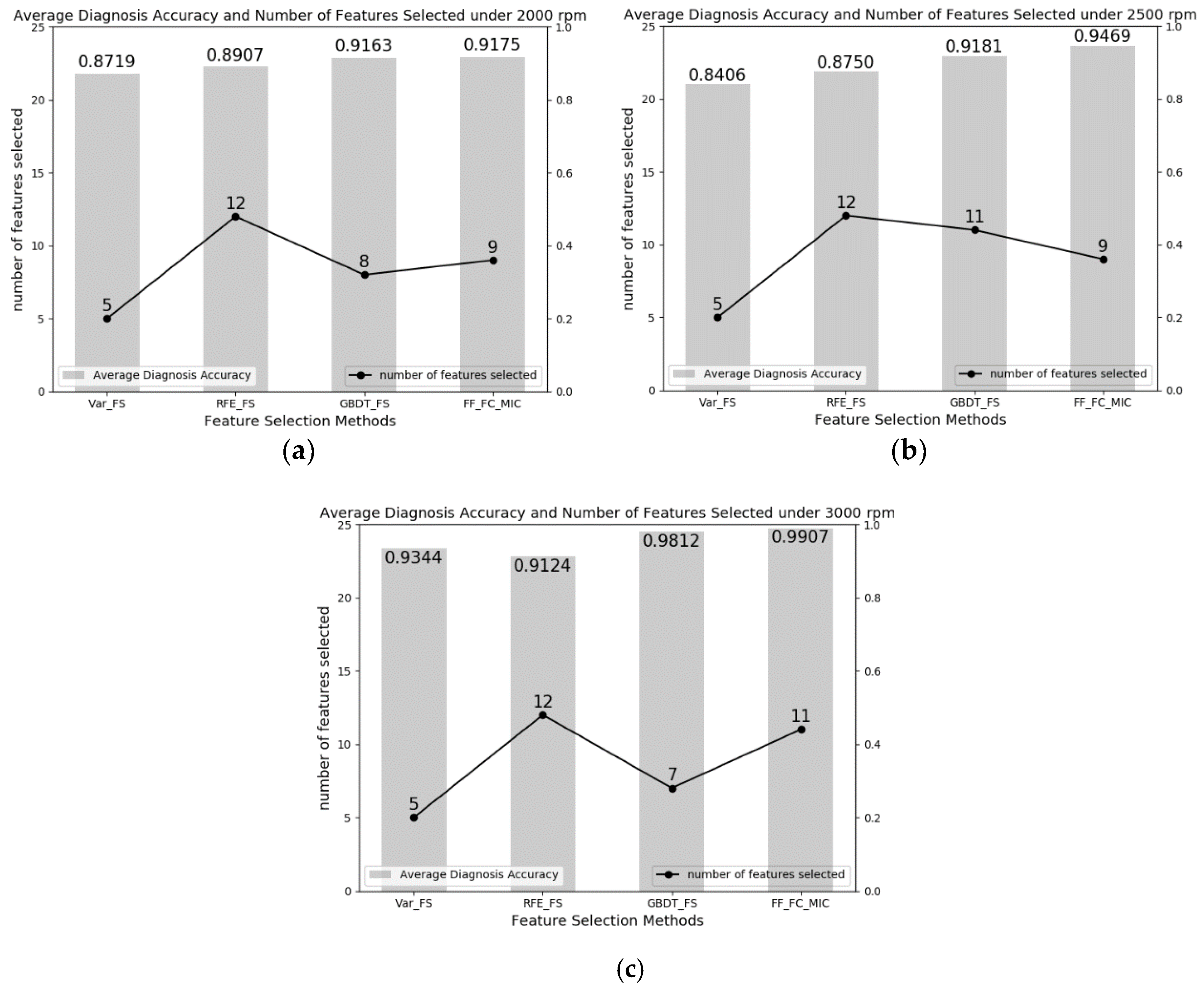
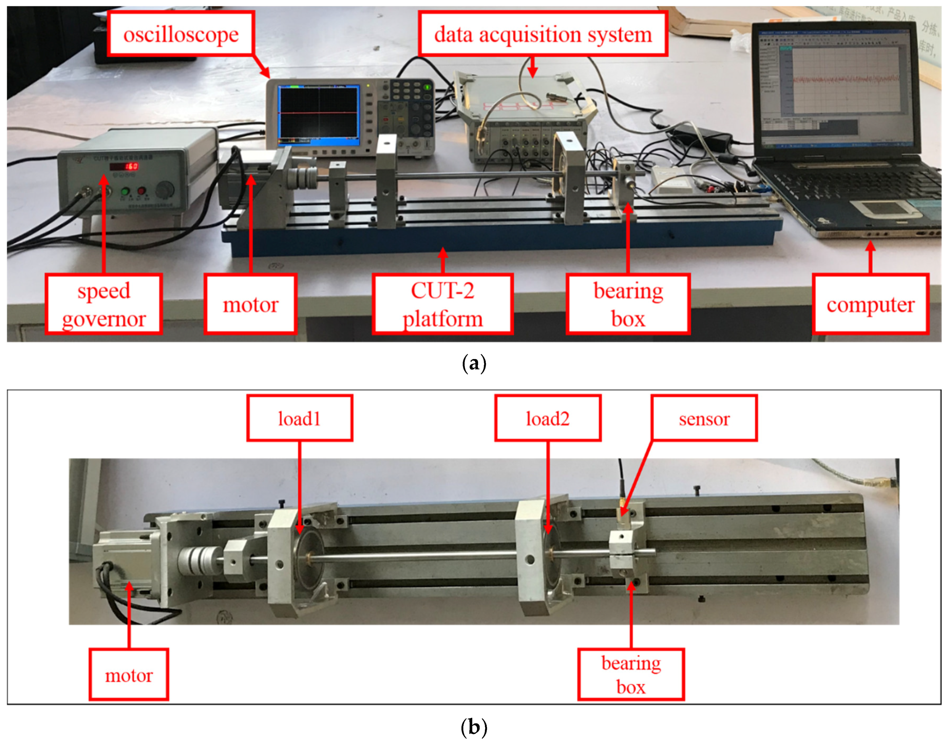
4.2. Experiments on CUT-2 Datasets

In order to validate the adaptability of the proposed feature selection method, vibration signals were collected and experiments were conducted on the CUT-2 platform. The whole experimental test rig is shown in Figure 4. The test rig was composed of an oscilloscope, a data acquisition system, a speed governor, a CUT-2 platform and a computer. All the measurements in the experimental system were carried out without load. In terms of vibration signal collection, the type of sensor was CT1010L, which is a kind of piezoelectric sensor, and the sensor was located in the horizontal direction of the bearing box. As shown in Figure 4b, the bearing tested in the experiment was placed at the far end of the motor. In addition, in order to validate the proposed method on the CUT-2 platform, an electric discharge machine was utilized to set three different kinds of faults. Figure 5 shows the bearing, of which the type was 6900ZZ in the experiments. The fault diameters were 0.2 mm and 0.3 mm. The vibration signals were collected by accelerometers at 3 different motor speeds of 2000 rpm, 2500 rpm and 3000 rpm, where the sampling frequency was 2 kHz.

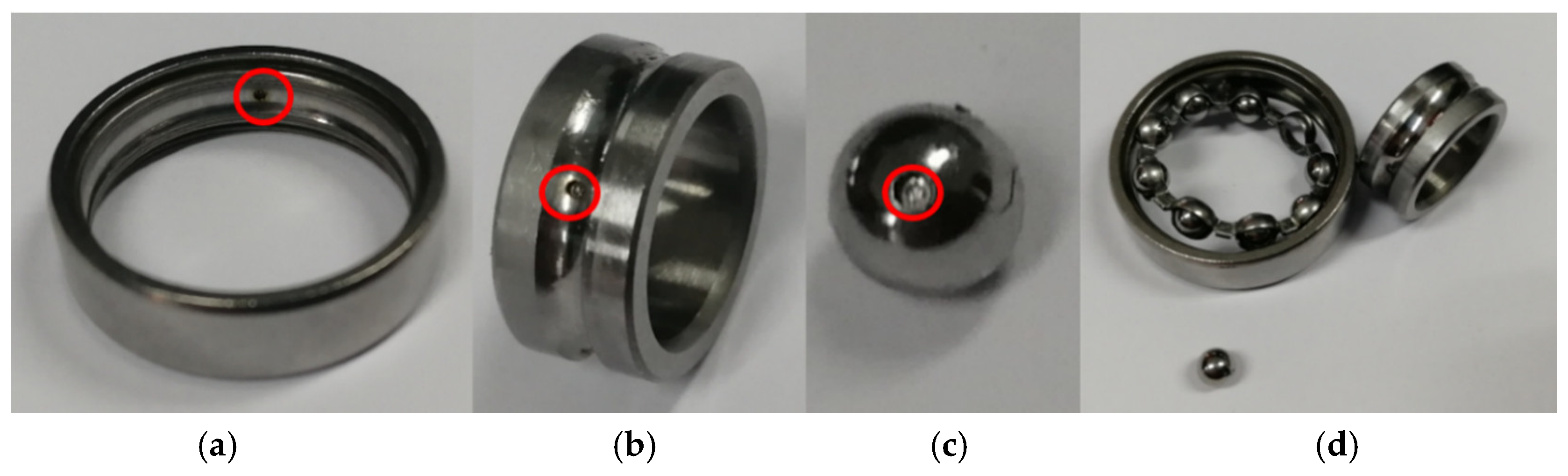
4.2.1. Experimental Setup and CUT-2 Datasets

In this section, the proposed method was applied on fault datasets from CUT-2. The details of the datasets are shown in Table 5. There were 4 kinds of bearing condition, including 1 normal condition and 3 fault conditions. The 3 fault conditions were inner race fault, outer race fault and baller fault. Two hundred samples were collected for each condition. Each sample contained 1024 continuous data points. Each dataset included 800 samples in total. Through data seeded, 3 kinds of datasets were acquired at 2000 rpm, 2500 rpm, and 3000 rpm. The training process and the testing process were carried out at the same speed. The training set included 560 samples and the testing set included 240 samples.

4.2.2. Result Analysis of CUT-2 Datasets

According to the proposed feature selection method, the features selected on 3 datasets are shown in Table 6. From Table 6, it can be seen that 9, 9 and 11 features were selected at 3 speeds.
Under most circumstances of 3 motor speeds from Table 7, the proposed feature selection method can reach the highest diagnosis accuracy, comparing to the other 3 methods. In addition, it performs a certain adaptability and stability on SVM and KNN.
At the speeds of 2000 rpm, 2500 rpm, and 3000 rpm, the average diagnosis accuracies are 91.75%, 94.69% and 99.07%, respectively. From this phenomenon, it was found that the diagnosis accuracy increases while the motor speed increases. There are 2 factors to cause this phenomenon. First, our bearings are small in both size and fault size, which means the vibration signal is less obvious in a lower speed than in a higher speed, leading to the phenomenon of a lower diagnosis accuracy in low speed and a higher diagnosis accuracy in high speed. Second, a large difference in motor speed, ranging from 2000 rpm to 3000 rpm, causes such a diversity of diagnosis accuracy increases while the motor speed increases.
For further analysis, compared with the other 3 methods, the proposed method can improve the accuracy by about an average of 1.32% at least, and by about an average of 6.94% at most. In term of diagnosis accuracy, the proposed method has a better performance than the other 3 feature selection methods.
In terms of number of features selected by different methods, the numbers of features selected among the 4 methods were compared. All the numbers of features selected by 4 methods are shown in Figure 6.

4.3. Comparison of Significant Differences

In this section, a comparison of significant differences was made to validate the proposed method. The proposed method was compared to each of the traditional feature selection method. Because of the reason that the experimental results were obtained based on small samples, the t-test was applied to test whether the mean difference between the two methods was significant. According to the t-test, the assumption that judges whether the expectations of two compared methods were equal was made:
H 0 :   μ 1 = μ 2 ,     H 1 :   μ 1 μ 2 .
If p-value < 0.05, the assumption will be accepted and it means the there is a significant difference between the two methods. If p-value > 0.05, the assumption will not be accepted and it means that there is not a significant difference between the two methods.
Table 8 shows that different p-values were calculated under the t-test. From Table 8, it is can be seen that under comparisons between each traditional method and the proposed method, the p-values of proposed method are all smaller than 0.05.
A conclusion can be drawn that the proposed method can achieve the highest diagnosis accuracy with fewer features and has a significant improvement in accuracy performance, compared with other 3 feature selection methods.

5. Conclusions

This paper presents a bearing fault diagnosis method based on the feature selection method called FF-FC-MIC by exploiting the capability of MIC to capture nonlinear relevance. The results can be summarized as follows: First, the most intuitive indicator, diagnosis accuracy, shows that the proposed method can reach 97.50%, and 98.75% in terms of average diagnosis accuracy in the CWRU dataset, and reach 91.75%, 94.69%, and 99.07% in terms of average diagnosis accuracy in the CUT-2 dataset. All the accuracies are the highest compared with those in the other feature selection methods. Second, on the basis of relevance among features and relevance between features and categories, the proposed method can select relatively low-dimension feature subsets to approach a higher diagnosis accuracy, compared with the other feature selection methods. Third, by calculating p-values under the t-test, the proposed method has a significant performance improvement, compared with traditional feature selection methods. The reasons can be summarized as follows: First, since the proposed method utilizes the MIC to measure the nonlinear and non-functional relationships between features and features, and between features and categories, it can eliminate redundant and irrelevant features. Second, the proposed method employs the intersection operation to merge two subsets, avoiding subset searching. Third, extensive experiments on the CWRU dataset and CUT-2 dataset were conducted to validate the effectiveness and adaptability of the proposed method. It turns out that the proposed method performs better in both reducing feature dimensions and achieving higher diagnosis accuracy, compared with the other 3 feature selection methods.
The relationship between the weight of features and feature subset is as essential as the work of feature selection. Besides, feature fusion technology should also be taken into consideration for feature selection. Our next work would investigate the relationship between the weight of features and feature subset and feature fusion technology to present more effective feature selection methods to reach the higher diagnosis accuracy.

Author Contributions

Conceptualization, X.T. and J.W.; methodology, J.W. and X.T.; software, J.W.; validation, X.T. and J.W.; investigation, X.T. and J.W.; data curation, J.W.; writing of original draft preparation, X.T. and J.W.; writing of review and editing, X.T., J.W., J.L., G.L. and J.C.; visualization, J.W.; supervision, X.T., J.L., G.L., and J.C.

Funding

This research was funded by Science and Technology Major Project of Guizhou Province ([2013]6019) and Project of Guizhou High-Level Study Abroad Talents Innovation and Entrepreneurship (2018.0002), Open Fund of Guizhou Provincial Public Big Data Key Laboratory (2017BDKFJJ019), and Guizhou University Foundation for the introduction of talent ((2016) No. 13).

Acknowledgments

We gratefully acknowledge the support of Jianjun Hu with the guiding for this research.

Conflicts of Interest

The authors declare no conflicts of interest.

References

  1. Ciabattoni, L.; Ferracuti, F.; Freddi, A.; Monteriu, A. Statistical Spectral Analysis for Fault Diagnosis of Rotating Machines. IEEE Trans. Ind. Electron. 2018, 65, 4301–4310. [Google Scholar] [CrossRef]
  2. Tra, V.; Kim, J.; Khan, S.A.; Kim, J. Bearing Fault Diagnosis under Variable Speed Using Convolutional Neural Networks and the Stochastic Diagonal Levenberg-Marquardt Algorithm. Sensors 2017, 17, 2834. [Google Scholar] [CrossRef] [PubMed]
  3. Rodriguez-Galiano, V.F.; Luque-Espinar, J.A.; Chica-Olmo, M.; Mendes, M.P. Feature selection approaches for predictive modelling of groundwater nitrate pollution: An evaluation of filters, embedded and wrapper methods. Sci. Total Environ. 2018, 624, 661–672. [Google Scholar] [CrossRef] [PubMed]
  4. Li, Y.; Li, T.; Liu, H. Recent advances in feature selection and its applications. Knowl. Inf. Syst. 2017, 53, 551–577. [Google Scholar] [CrossRef]
  5. Kashef, S.; Nezamabadi-Pour, H.; Nikpour, B. Multilabel feature selection: A comprehensive review and guiding experiments. Wiley Interdiscip. Rev.: Data Min. Knowl. Discov. 2018, 8, e1240. [Google Scholar] [CrossRef]
  6. Yao, X.; Wang, X.; Zhang, Y.; Quan, W. Summary of feature selection algorithms. Control. Decis. 2012, 27, 161–313. [Google Scholar]
  7. Fu, X.; Zhang, Y.; Zhu, Y. Rolling bearing fault diagnosis approach based on case-based reasoning. J. Xi’an Jiaotong Univ. 2011, 45, 79–84. [Google Scholar]
  8. Ou, L.; Yu, D. Rolling bearing fault diagnosis based on supervised laplaian score and principal component analysis. J. Mech. Eng. 2014, 88–94. [Google Scholar] [CrossRef]
  9. Ou, L.; Yu, D. Rolling bearing fault diagnosis based on laplaian score fuzzy C-means clustering. China Mech. Eng. 2014, 25, 1352–1357. [Google Scholar]
  10. Hui, K.H.; Ooi, C.S.; Lim, M.H.; Leong, M.S.; Al-Obaidi, S.M. An improved wrapper-based feature selection method for machinery fault diagnosis. PLOS ONE 2017, 12, e189143. [Google Scholar] [CrossRef] [PubMed]
  11. Liu, X.; Zheng, H.; Zhu, T. Feature selection in machine fault diagnosis based on evolutionary Monte Carlo method. J. Vib. Shock 2011, 30, 98–101. [Google Scholar]
  12. Islam, R.; Khan, S.A.; Kim, J. Discriminant Feature Distribution Analysis-Based Hybrid Feature Selection for Online Bearing Fault Diagnosis in Induction Motors. J. Sens. 2016, 2016, 1–16. [Google Scholar] [CrossRef]
  13. Luo, M.; Li, C.; Zhang, X.; Li, R.; An, X. Compound feature selection and parameter optimization of ELM for fault diagnosis of rolling element bearings. ISA Trans. 2016, 65, 556–566. [Google Scholar] [CrossRef] [PubMed]
  14. Yu, X.; Dong, F.; Ding, E.; Wu, S.; Fan, C. Rolling Bearing Fault Diagnosis Using Modified LFDA and EMD with Sensitive Feature Selection. IEEE Access 2018, 6, 3715–3730. [Google Scholar] [CrossRef]
  15. Liu, Y.; Hu, J.; Ren, L.; Yao, K.; Duan, J.; Chen, L. Study on the Bearing Fault Diagnosis based on Feature Selection and Probabilistic Neural Network. J. Mech. Transm. 2016, 40, 48–53. [Google Scholar]
  16. Yang, Y.; Pan, H.; Wei, J. The rolling bearing fault diagnosis method based on the feature selection and RRVPMCD. J. Vib. Eng. 2014, 27, 629–636. [Google Scholar]
  17. Atamuradov, V.; Medjaher, K.; Camci, F.; Dersin, P.; Zerhouni, N. Railway Point Machine Prognostics Based on Feature Fusion and Health State Assessment. IEEE Trans. Instrum. Meas. 2018, 1–14. [Google Scholar] [CrossRef]
  18. Cui, B.; Pan, H.; Wang, Z. Fault diagnosis of roller bearings base on the local wave and approximate entropy. J. North University China (Nat. Sci. Ed.) 2012, 33, 552–558. [Google Scholar]
  19. Shi, L. Correlation Coefficient of Simplified Neutrosophic Sets for Bearing Fault Diagnosis. Shock. Vib. 2016, 2016, 1–11. [Google Scholar] [CrossRef]
  20. Zheng, J.; Cheng, J.; Yang, Y.; Luo, S. A rolling bearing fault diagnosis method based on multi-scale fuzzy entropy and variable predictive model-based class discrimination. Mech. Mach. Theory 2014, 78, 187–200. [Google Scholar] [CrossRef]
  21. Zhang, N.; Wu, L.; Yang, J.; Guan, Y. Naive Bayes Bearing Fault Diagnosis Based on Enhanced Independence of Data. Sensors 2018, 18, 463. [Google Scholar] [CrossRef] [PubMed]
  22. Jiang, X.; Wu, L.; Ge, M. A Novel Faults Diagnosis Method for Rolling Element Bearings Based on EWT and Ambiguity Correlation Classifiers. Entropy 2017, 19, 231. [Google Scholar] [CrossRef]
  23. Wang, Y.; Feng, L. Hybrid feature selection using component co-occurrence based feature relevance measurement. Expert Syst. Appl. 2018, 102, 83–99. [Google Scholar] [CrossRef]
  24. Bharti, K.K.; Singh, P.K. Hybrid dimension reduction by integrating feature selection with feature extraction method for text clustering. Expert Syst. Appl. 2015, 42, 3105–3114. [Google Scholar] [CrossRef]
  25. Xu, J.; Huang, F.; Mu, H.; Wang, Y.; Xu, Z. Tumor feature gene selection method based on PCA and information gain. J. Henan Univ. (Nat. Sci. Ed.) 2018, 46, 104–110. [Google Scholar]
  26. Zhu, L.; Wang, X.; Zhang, J. An engine fault diagnosis method based on ReliefF-PCA and SVM. J. Beijing Univ. Chem. Technol. (Nat. Sci.) 2018, 45, 55–59. [Google Scholar]
  27. Xiao, Y.; Liu, C. Improved PCA method for SAR target recognition based on sparse solution. J. Univ. Chin. Acad. Sci. 2018, 35, 84–88. [Google Scholar]
  28. Du, Z.; Xiang, C. A Wavelet Packet Decomposition and Principal Component Analysis Approach. Control Eng. China 2016, 23, 812–815. [Google Scholar]
  29. Fadda, M.L.; Moussaoui, A. Hybrid SOM–PCA method for modeling bearing faults detection and diagnosis. J. Braz. Soc. Mech. Sci. Eng. 2018, 40. [Google Scholar] [CrossRef]
  30. Wang, T.; Xu, H.; Han, J.; Elbouchikhi, E.; Benbouzid, M.E.H. Cascaded H-Bridge Multilevel Inverter System Fault Diagnosis Using a PCA and Multiclass Relevance Vector Machine Approach. IEEE Trans. Power Electron. 2015, 30, 7006–7018. [Google Scholar] [CrossRef]
  31. Sun, G.; Song, Z.; Liu, J.; Zhu, S.; He, Y. Feature Selection Method Based on Maximum Information Coefficient and Approximate Markov Blanket. Acta Autom. Sin. 2017, 43, 795–805. [Google Scholar]
  32. The Case Western Reserve University Bearing Data Center Bearing Data Center Seeded Fault Test Data[EB/OL]. Available online: http://csegroups.case.edu/bearingdatacenter/pages/download-data-file (accessed on 10 June 2016).
  33. Wei, Z.; Wang, Y.; He, S.; Bao, J. A novel intelligent method for bearing fault diagnosis based on affinity propagation clustering and adaptive feature selection. Knowl.-Based Syst. 2017, 116, 1–12. [Google Scholar] [CrossRef]
  34. Lei, Y.; He, Z.; Zi, Y. Fault Diagnosis Based on Novel Hybrid Intelligent Model. Chin. J. Mech. Eng. 2008, 44, 112–117. [Google Scholar] [CrossRef]
Figure 1. Flowchart of the proposed method. (a) Data preprocessing: Features are obtained through the time domain and frequency domain, forming a feature set ( F S ) matrix with a size of n × m ; (b) MIC (Maximum Information Coefficient) calculation: relevance between features and features are calculated to obtain an FF-MIC matrix with a size of m × m by MIC, and relevance between features and fault categories are calculated to obtain the FC-MIC matrix with a size of m × p by MIC; (c) relevance calculation: a threshold F F _ t h r e s h o l d is set to distinguish strong irrelevance features from F S , and a threshold F C _ t h r e s h o l d is set to distinguish strong relevance features from F S ; (d) obtaining of feature subsets: according to the thresholds, Subset1 and Subset2 are obtained; (e) merging of feature subsets: An intersection operation is applied to merge Subset1 and Subset2, obtaining a final subset F S u b s e t ; (f) PCA: PCA is employed to further reduce the dimension of F S u b s e t .
Applsci 08 02143 g001
Figure 2. CWRU bearing experimental platform.
Applsci 08 02143 g002
Figure 3. Average diagnosis accuracy of single fault and number of features selected at two motor speeds. (a) Average diagnosis accuracy and number of features selected at 1750 rpm; (b) average diagnosis accuracy and number of features selected at 1772 rpm.
Applsci 08 02143 g003
Figure 4. Experimental test rig: (a) CUT-2 data acquisition system; (b) CUT-2 platform.
Applsci 08 02143 g004
Figure 5. Locations of bearing faults: (a) outer race fault; (b) ball fault; (c) inner race fault; and (d) combination of parts.
Applsci 08 02143 g005
Figure 6. Average diagnosis accuracy of fault and number of features selected at three motor speeds: (a) average diagnosis accuracy and number of features selected at the speed of 2000 rpm; (b) average diagnosis accuracy and number of features selected at the speed of 2500 rpm; (c) average diagnosis accuracy and number of features selected at the speed of 3000 rpm.
Applsci 08 02143 g006
Table 1. Features in the time domain and frequency domain [14,33,34].
Features in the Time DomainFeatures in the Frequency Domain
f 0 = n = 1 N x ( n ) N f 6 = n = 1 N ( x ( n ) f 0 ) 4 ( N 1 ) f 2 4 f 12 = k = 1 K s ( k ) K f 19 = k = 1 K f k 4 s ( k ) k = 1 K f k 2 s ( k )
f 1 = n = 1 N ( x ( n ) ) 2 N 1 f 7 = f 4 f 3 f 13 = k = 1 K ( s ( k ) f 12 ) 2 K 1 f 20 = k = 1 K f k 2 s ( k ) k = 1 K s ( k ) k = 1 K f k 4 s ( k )
f 2 = ( n = 1 N | x ( n ) | N ) 2 f 8 = f 4 f 2 f 14 = k = 1 K ( s ( k ) f 12 ) 3 K ( f 13 ) 3 f 21 = f 17 f 16
f 3 = n = 1 N ( x ( n ) ) 2 N f 9 = f 3 1 N n = 1 N | x ( n ) | f 15 = k = 1 K ( s ( k ) f 12 ) 4 K ( f 13 ) 2 f 22 = k = 1 K ( f k f 16 ) 3 s ( k ) K f 17 3
f 4 = max | x ( n ) | f 10 = f 4 1 N n = 1 N | x ( n ) | f 16 = k = 1 K f k s ( k ) k = 1 K s ( k ) f 23 = k = 1 K ( f k f 16 ) 4 s ( k ) K f 17 4
f 5 = n = 1 N ( x ( n ) f 1 ) 3 ( N 1 ) f 2 3 f 11 = n = 1 N | x ( n ) | 2 f 17 = k = 1 K ( f k f 16 ) 2 s ( k ) K f 24 = k = 1 K ( f k f 16 ) 1 / 2 s ( k ) K f 17
f 18 = k = 1 K f k 2 s ( k ) k = 1 K s ( k )
x ( n ) is the time-domain signal sequence, n = 1 , 2 , , N , N is the number of each sample points. s ( k ) is the frequency-domain signal sequence, k = 1 , 2 , , K , K is the number of spectral lines.
Table 2. Datasets obtained at the motor speeds of 1750 rpm and 1772 rpm on the CWRU bearing experimental platform.
Conditions of the BearingsFault Size (inch)Number of SamplesClass
Normal 1500
Inner race fault0.007501
0.01450
0.02150
Outer race fault0.007502
0.01450
0.02150
Baller fault0.007503
0.01450
0.02150
Table 3. CWRU dataset features selected by the proposed method. (The pictures are the visualization results for the corresponding speed samples. The horizontal axis in the figure represents the number of features, and the vertical axis represents the first 13 samples. For the sake of beauty, the first 13 samples are chosen).
Motor Speed (rpm)All FeaturesSelected FeaturesSelected Number
1750 Applsci 08 02143 i001 Applsci 08 02143 i0020, 3, 8, 9, 11, 16, 22
1772 Applsci 08 02143 i003 Applsci 08 02143 i0040, 3, 8, 9, 11, 15, 16, 20, 22
Table 4. Comparison of classification accuracy of SVM and KNN at motor speeds of 1750 rpm and 1772 rpm using different feature selection methods.
Motor Speed (rpm)Feature Selection MethodsClassification Models
SVMKNN
1750Var_FS0.87500.8750
RFE_FS0.85000.8333
GBDT_FS0.94170.9600
FF_FC_MIC0.95830.9750
1772Var_FS0.77500.7417
RFE_FS0.80000.7666
GBDT_FS0.98330.9917
FF_FC_MIC0.99171.0000
Table 5. Datasets obtained at motor speeds of 2000 rpm, 2500 rpm and 3000 rpm on the CUT-2 platform.
Conditions of the BearingsFault Size (mm)Number of SamplesClass
Normal condition 2000
Inner race fault0.2
0.3
100
100
1
Outer race fault0.2
0.3
100
100
2
Baller fault0.2
0.3
100
100
3
Table 6. Dataset features selected by the proposed method. (The pictures are the visualization results for the corresponding speed samples. The horizontal axis in the figure represents the number of features, and the vertical axis represents the first 13 samples. For the sake of beauty, the first 13 samples are chosen).
Motor Speed (rpm)All FeaturesSelected FeaturesSelected Number
2000 Applsci 08 02143 i005 Applsci 08 02143 i0060, 2, 3, 8, 10, 11, 19, 20, 22
2500 Applsci 08 02143 i007 Applsci 08 02143 i008
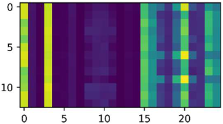
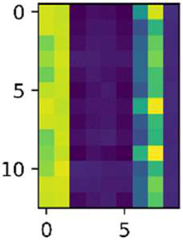
0, 3, 8, 9, 10, 11, 19, 20, 22
3000 Applsci 08 02143 i009 Applsci 08 02143 i010
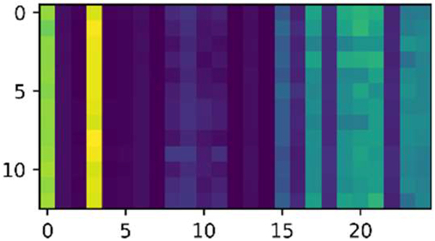
0, 3, 8, 9, 11, 14, 15, 16, 20, 21, 23
Table 7. Comparison of classification accuracy of SVM and KNN at motor speeds of 2000 rpm, 2500 rpm and 3000 rpm using different feature selection methods.
Motor Speed (rpm)Feature Selection MethodsClassification Models
SVMKNN
2000Var_FS0.86880.8750
RFE_FS0.89380.8875
GBDT_FS0.93130.9012
FF_FC_MIC0.92250.9125
2500Var_FS0.85620.8250
RFE_FS0.86880.8812
GBDT_FS0.91870.9175
FF_FC_MIC0.96250.9313
3000Var_FS0.94370.9250
RFE_FS0.91870.9062
GBDT_FS0.97500.9875
FF_FC_MIC0.99380.9875
Table 8. Comparison between traditional feature selection methods and the proposed method.
Methods Comparedp-ValueWhether the Mean Difference between the Two Methods Is Significant (Y/N)
Var_FS, FF_FC_MIC1.166 × 10 3 Y
RFE_FS, FF_FC_MIC2.509 × 10 5 Y
GBDT_FS, FF_FC_MIC3.576 × 10 2 Y

