A Robotic Drilling End-Effector and Its Sliding Mode Control for the Normal Adjustment

Featured Application

Robotic Drilling.

Abstract

A robotic drilling end-effector is designed and modeled, and a sliding mode variable structure control architecture based on the reaching law is proposed for its normal adjustment dynamic control. By using a third-order nonlinear integration chain differentiator for obtaining the unmeasurable speed and acceleration signals from the position signals, this sliding mode control scheme is developed with good dynamic quality. The new control law ensures global stability of the entire system and achieves both stabilization and tracking within a desired accuracy. A real-time control experiment platform is established in xPC target environment based on MATLAB Real-Time Workshop (RTW) to verify the proposed control scheme and simulation results. Simulations and experiments performed on the designed robotic end-effector illustrate and clarify that the proposed control scheme is effective.

1. Introduction

Robots have undoubtedly demonstrated their value in the automotive industry, they have been regarded suitable for aerospace applications such as drilling and fastening due to the obvious low investment costs compared to bespoke industrial solutions [1]. The traditional application areas for industrial robots involve highly repetitive operations such as drilling. Robotic drilling system has made extensive application in both industry and research field. In the aircraft industry, where the drilling of many thousands of holes per aircraft is needed, the usually adopted solution is to stack the parts in a joint position and drill them in a single operation [2,3]. The use of industrial robots for drilling is gaining an increasing interest due to their flexibility and the comparatively low cost of industrial robot systems [4,5]. DeVlieg et al. [6] and Atkinson et al. [7] developed a drilling system for the skin to substructure joint on the F/A-18E/F Super Hornet wing trailing edge flaps (TEF) and for 737 Aileron, which utilizes a mass produced, high capacity industrial robot such as Kuka KR350/2 and KR360-2 as the motion platform for an automated drilling, countersinking, and hole inspection machine.

In general, a servo-controlled robotic drilling end-effector is coupled with an industrial robot to complete the drilling process. Webb et al. [8] developed a compact and innovative end-effector which is capable of performing drilling, countersinking, sealing and riveting operations and also contains a significant amount of process monitoring sensors to enable automated in-process checks and quality measurement. Hempstead et al. [9] developed an end-effector for use on a Kuka KR350 robot. The end-effector pushes up on a wing panel with programmable pressure, drills a hole with a servo drill, inspects the hole with a servo ball-type hole gauge and then drives a pin-tail style lock bolt into the hole. Liang et al. [10] further designed a drilling end-effector to use for industrial robots. The real-time force feedback can detect dull or broken bits, drill to breakthrough, and plot thrust force while drilling. Devlieg [11] also developed a single process end-effector that performs all required functions, including one-sided pressure application, touch probing, barcode scanning, drilling/countersinking, measurement of hole diameter and countersink depth, and face milling. Automatic drilling requires the drilling bit to be perpendicular to the curved surface of fuselage. However, most of these references focus exclusively on all-in-one end-effector structure design and functions such as drilling, countersinking, inspecting or monitoring, and fastening [12], and a few on the normal adjustment dynamical model and control. The development of these robotic drilling systems has created a research need for the dynamical models and control of the normal adjustment of robotic drilling end-effector.

The dynamic performance of the normal adjustment of the robotic drilling end-effector will affect the drilling quality and productivity. Olsson [13] presented methods and systems for force-controlled robot drilling, based on active suppression of drill sliding through a model-based force control scheme. Tian et al. [14] proposed a novel approach based on the detection system to detect the normal vector to product surface in real time for the robotic precision drilling system in aircraft component assembly. Mei et al. [15] proposed a novel in-process robot base frame calibration method with a 2D vision system to measure and compensate the position errors of drilled fastener holes. Frommknecht [16] presented a multi-sensor measurement system for robotic drilling. The system enables a robot to measure its 6D pose with respect to the work piece and to establish a reference coordinate system for drilling. Shi et al. [5] developed a normal adjustment cell (NAC) in aero-robotic drilling by using an intelligent double-eccentric disk normal adjustment mechanism (2-EDNA), a spherical plain bearing, and a floating compress module with sensors to improve the quality of vertical drilling. Qin et al. [17] presented an approach for the acquisition of vibration signals of the end-effector in robotic drilling. With the aid of the rigid body kinematics, the vibration signals of the end-effector can be obtained and analyzed. Garnier et al. [18] proposed two robotic drilling models, in which the cutting process and the stiffness of the robot hand are taken into account, respectively. However, these efforts focus basically on kinematics analysis and static accuracy insurance, depending quite a bit on sensors. Though Zhang et al. [19] proposed an intelligent surface-normal adjustment system to deal with the normal adjustment that focused on calculating surface-normal vector to regulate the feed direction of the drilling bit in real-time, this works didn’t involve the dynamic characteristics of the normal adjustment of the end-effector.

This paper develops a robotic drilling end-effector for industrial robot. Based on the dynamics modeling and analysis, a sliding mode variable structure control architecture with the constant plus exponential rate reaching law is proposed for the normal adjustment dynamic control. By using a third-order nonlinear integration chain differentiator for obtaining the unmeasurable speed and acceleration signals from the position signals with the minimum noise, this sliding mode control scheme is developed with good dynamic quality. The new control law ensures global stability of the entire system and achieves both stabilization and tracking within a desired precision. A real-time control experiment platform is established in xPC target environment based on MATLAB Real-Time Workshop (RTW) to verify the proposed control scheme and simulation results. Simulations and experiments performed on the designed robotic end-effector illustrate and clarify that the controller is effective and robust.

2. Dynamical Model for the Robotic Drilling End-Effector

2.1. The Structure of the Robotic Drilling End-Effector

The main functions of the designed robotic drilling end-effector include: measuring and calculating the outward normal of the fuselage surface at drilling point, adjusting spindle axis to coincide with the normal and drilling after the surface is reliably compressed. A diagram and a photograph of the designed robotic drilling end-effector are shown in Figure 1. Figure 1a shows a diagram of the end-effector structure, Figure 1b shows the specifics of the internal structure of the end-effector, and Figure 1c shows the prototype of the end-effector, in which the spindle and feed units fulfill spindle driving and feeding. The compressing unit compresses the surface to diminish the vibration during the drilling process. It also helps to eliminate the clearances between the layers of material in order to avoid chips going into layers and causing stress concentration. There are four displacement sensors arranged evenly in the compressing unit around the spindle for measuring four space coordinates on the surface around drilling area. Thus, by the proposed method of measuring and calculating the normal of curved surface [19], the outward normal of fuselage surface at drilling point is obtained. The normal adjusting unit is fixed on the frame, and two mutually perpendicular axes (Joints 1 and 2) are installed in a plane normal to the spindle. The spindle can rotate about these two axes, thus fulfilling the function of adjusting the spindle to normal of the surface. The frame links and supports above parts, and connects the end-effector to robot.

2.2. Motion Equations of the Robotic Drilling End-Effector

The coordinate system of the designed robotic drilling end-effector is shown as Figure 2. The kinematic model is established using Denavit-Hartenberg (D-H) method. The base coordinate system is placed in rotating Joint 1 and concentric exactly with joint coordinate {1}. Because the normal adjustment unit of the end-effector consists of Joints 1 and 2, the world frame {0} is placed at the center of the Joint 1 and is concentric with the frame {1} for the sake of analysis.

The transform matrixes in the coordinate system are calculated as:

$${}_1{}^{0}T=\left[\begin{array}{cccc}\cos {\theta }_1& -\sin {\theta }_1& 0& 0\\ \sin {\theta }_1& \cos {\theta }_1& 0& 0\\ 0& 0& 1& 0\\ 0& 0& 0& 1\end{array}\right]$$

(1)

$${}_2{}^{1}T=\left[\begin{array}{cccc}-\sin {\theta }_2& -\cos {\theta }_2& 0& 0\\ 0& 0& 1& 0\\ -\cos {\theta }_2& \sin {\theta }_2& 0& 0\\ 0& 0& 0& 1\end{array}\right]$$

(2)

$${}_3{}^{2}T=\left[\begin{array}{cccc}0& -1& 0& 0\\ 0& 0& -1& d_3\\ 1& 0& 0& 0\\ 0& 0& 0& 1\end{array}\right].$$

(3)

Both spindle feeding unit and pressing unit will not move in the normal adjusting process of the end-effector. Thus, both their acceleration and velocity are 0.

A 3 × 3-order positive definite inertial matrix is calculated as:

$$D\left(q\right)=\left[\begin{array}{ccc}{D}_{11}& D_{12}& D_{13}\\ D_{21}& D_{22}& D_{23}\\ D_{31}& D_{32}& D_{33}\end{array}\right]$$

(4)

with

$$q={\left[\begin{array}{ccc}{\theta }_1& {\theta }_2& d_3\end{array}\right]}^T$$

(5)

$$\begin{array}{l}{D}_{11}=I_{zz1}+I_{yy2}+I_{zz3}+I_{a1}+(I_{xx2}-I_{yy2}+I_{yy3}-I_{zz3}-2m_3{d}_3{c}_{z3}+m_3{d}_3^2){\cos }^2\left({\theta }_2\right)\\ \hspace{1em}\hspace{1em}+\left(I_{xy2}+I_{yz3}-m_3{d}_3{c}_{y3}\right)\sin \left(2{\theta }_2\right)\hfill \end{array}$$

(6)

$$D_{12}=\left(-I_{yz2}+I_{xz3}-m_3{d}_3{c}_{x3}\right)\sin \left({\theta }_2\right)+\left(I_{xz3}-I_{xy3}\right)\cos \left({\theta }_2\right)$$

(7)

$$D_{13}=m_3{c}_{x3}\cos \left({\theta }_2\right)$$

(8)

$$D_{21}=\left(-I_{yz2}+I_{xz3}-m_3{d}_3{c}_{x3}\right)\sin \left({\theta }_2\right)+\left(I_{xz2}-I_{xy3}\right)\cos \left({\theta }_2\right)$$

(9)

$$D_{22}=I_{zz2}+I_{xx3}-2m_3{d}_3{c}_{z3}+m_3{d}_3^2+I_{a2}$$

(10)

$$D_{23}=-m_3{c}_{y3}$$

(11)

$$D_{31}=m_3{c}_{x3}\cos \left({\theta }_2\right)$$

(12)

$$D_{32}=-m_3{c}_{y3}$$

(13)

$$D_{33}=m_3+I_{a3}$$

(14)

where θ₁ and θ₂ denote the rotation angles of the Joints 1 and 2, respectively, and d₃ denotes the linear displacement of the prismatic Joint 3. I_abi is the product of inertia of Joint i with respect to a pair of orthogonal axes a and b, a, b denote x, y, or z; m_i is the mass of Joint i. c_ai is the centroid coordinate of Joint i on axis a, a denote x, y, or z.

A 3 × 1-order vector of centrifugal and Coriolis force is calculated, regarding that ${\dot{q}}_3={\dot{d}}_3=0$, the result is:

$$H\left(q,\dot{q}\right)={\left[\begin{array}{ccc}{h}_1& h_2& h_3\end{array}\right]}^T$$

(15)

with

$$\begin{array}{l}{h}_1=[\left(-I_{xx2}+I_{yy2}-I_{yy3}+I_{zz3}-m_3{d}_3^2+2m_3{d}_3{c}_{z3}\right)\sin \left(2{\theta }_2\right)+2\left(I_{xy2}+I_{yz3}-m_3{d}_3{c}_{y3}\right)\cos \left(2{\theta }_2\right)]{\dot{\theta }}_1{\dot{\theta }}_2\\ \hspace{1em}+\left[\left(-I_{xz2}+I_{xy3}\right)\sin \left({\theta }_2\right)+\left(-I_{yz2}+I_{xz3}-m_3{d}_3{c}_{x3}\right)\cos \left({\theta }_2\right)\right]{\dot{\theta }}_2^2\end{array}$$

(16)

$$h_2=[\frac{1}{2}\left(I_{xx2}-I_{yy2}+I_{yy3}-I_{zz3}-2m_3{d}_3{c}_{z3}+m_3{d}_3^2\right)\sin \left(2{\theta }_2\right)+\left(-I_{xy2}-I_{yz3}+m_3{d}_3{c}_{y3}\right)\cos \left(2{\theta }_2\right)]{\dot{\theta }}_1^2$$

(17)

$$h_3=m_3\cos \left({\theta }_2\right)\left[c_{y3}\sin \left({\theta }_2\right)+\left(c_{z3}-d_3\right)\cos \left({\theta }_2\right)\right]{\dot{\theta }}_1^2+m_3\left(c_{z3}-d_3\right){\dot{\theta }}_2^2.$$

(18)

A 3 × 1-order gravity vector is calculated as:

$$G\left(q\right)=\left[\begin{array}{ccc}{G}_1& G_2& G_3\end{array}\right]$$

(19)

with

$$\begin{array}{l}{G}_1=[m_1{c}_{x1}\sin \left({\theta }_1\right)+\left(m_1{c}_{y1}+m_2{c}_{z2}+m_3{c}_{x3}\right)\cos \left({\theta }_1\right)+\left(-m_2{c}_{x2}+m_3{c}_{y3}\right)\sin \left({\theta }_1\right)\sin \left({\theta }_2\right)\\ \hspace{1em}+\left(-m_2{c}_{y2}+m_3{c}_{z3}-m_3{d}_3\right)\sin \left({\theta }_1\right)\cos \left({\theta }_2\right)]g\end{array}$$

(20)

$$G_2=[\left(-m_2{c}_{y2}+m_3{c}_{z3}-m_3{d}_3\right)\sin \left({\theta }_2\right)+\left(m_2{c}_{x2}-m_3{c}_{y3}\right)\cos \left({\theta }_2\right)]g\cos \left({\theta }_1\right)$$

(21)

$$G_3=m_{3}g\cos \left({\theta }_1\right)\cos \left({\theta }_2\right).$$

(22)

According to Lagrange’s equation, the dynamical equation of the end-effector is derived as:

$$D\left(q\right)\ddot{q}+H\left(q,\dot{q}\right)+G\left(q\right)=\mathsf{\tau }$$

(23)

or

$$\left[\begin{array}{ccc}{D}_{11}& D_{12}& D_{13}\\ D_{21}& D_{22}& D_{23}\\ D_{31}& D_{32}& D_{33}\end{array}\right]\left[\begin{array}{c}{\ddot{\theta }}_1\\ {\ddot{\theta }}_2\\ {\ddot{d}}_3\end{array}\right]+\left[\begin{array}{c}{h}_1\\ h_2\\ h_3\end{array}\right]+\left[\begin{array}{c}{G}_1\\ G_2\\ G_3\end{array}\right]=\left[\begin{array}{c}{\tau }_1\\ {\tau }_2\\ f_3\end{array}\right]$$

(24)

where τ₁ and τ₂ denote the torque acting on Joints 1 and 2, respectively, f₃ denotes the force acting on prismatic Joint 3.

The joint parameters of the end-effector calculated by the model are listed in

Table 1. Joint parameters of the end-effector.

Parameters	i = 1	i = 2	i = 3
Ixxi (m4)	0.03	0.04	0.03
Ixyi (m4)	0	0.01	0
Ixzi (m4)	0	−0.01	0
Iyxi (m4)	0	0.01	0
Iyyi (m4)	0.09	0.11	0.04
Iyzi (m4)	0	0	0
Izxi (m4)	0	−0.11	0
Izyi (m4)	0	0	0
Izzi (m4)	0.06	0.11	0.01
mi (kg)	5.8	7.6	8.6
cxi (m)	0.05	0.02	0
cyi (m)	0	0.02	0
czi (m)	0	−0.01	0.14

.

3. Sliding Mode Controller Design

3.1. Friction Compensation

In order to research dynamical characteristic of the end-effector during normal orientation adjusting, considering that feed unit and compressing unit maintain resting state during the normal adjusting process, Equation (23) is rewritten as:

$$D\left(\Theta \right)\ddot{\Theta }+H\left(\Theta ,\dot{\Theta }\right)+G\left(\Theta \right)=\mathsf{\tau }$$

(25)

where $\Theta ={\left[\begin{array}{cc}{\theta }_1& {\theta }_2\end{array}\right]}^T$ and $\mathsf{\tau }={\left[\begin{array}{cc}{\tau }_1& {\tau }_2\end{array}\right]}^T$.

Equation (25) is an ideal dynamical model, because it didn’t take into account the effects of friction torque and disturbing torque on the joints. Friction is a phenomenon with obvious nonlinearity that remains ubiquitous in mechanical systems. It always causes untoward consequences such as system steady-state error, limit cycle, static-slip and oscillation. Therefore, the friction torque and disturbing torque should be considered to obtain comparative control quality. The dynamical model needs to be modified as:

$$D\left(\Theta \right)\ddot{\Theta }+H\left(\Theta ,\dot{\Theta }\right)+G\left(\Theta \right)+F\left(\Theta ,\dot{\Theta },\ddot{\Theta }\right)+{\mathsf{\tau }}_d=\mathsf{\tau }$$

(26)

where $F\left(\Theta ,\dot{\Theta },\ddot{\Theta }\right)$ denotes friction torque while ${\mathsf{\tau }}_d$ denotes disturbing torque.

Therefore, in order to compensate the friction torque, it is necessary to establish a friction model to estimate the friction torque. Stribeck model is a classical friction model which has components that are either linear in velocity or constant and describes the mechanical characteristics of various friction stages. The resulting friction force F_f can be expressed as [20]:

$$F_f=\{\begin{array}{ll}F\left(v\right)& \mathrm{if}v\ne 0\\ F_e& \mathrm{if}v=0\mathrm{and}\left|F_e\right|<F_s\\ F_s\mathrm{sgn}\left(F_e\right)& \mathrm{other}\end{array}$$

(27)

$$F\left(v\right)=F_c+\left(F_s-F_c\right)e^{-{\left|v/v_s\right|}^2}+F_{v}v$$

(28)

where v is motion velocity; v_s is named Stribeck velocity; F_e denotes driving force; F_s denotes maximum static friction force; F_c denotes Coulomb friction force; F_v denotes viscous frictional torque coefficient. It is easy to identify the expression for F_f by measuring friction force in condition of uniform motion.

3.2. Sliding Mode Control Based on Model

Utilizing controller decomposition, a dynamic control law combining the linearized feedback of joints’ parameters and servo compensator is investigated. The feedback linearization method which is often called computed torque method is a kind of design method based on system dynamical model. Define the driving torque as Equation (29).

$$\mathsf{\tau }=\mathsf{\alpha }u+\mathsf{\beta }$$

(29)

with

$$\begin{gathered} \mathsf{\alpha }=D\left(\Theta \right) \\ \mathsf{\beta }=H\left(\Theta ,\dot{\Theta }\right)+G\left(\Theta \right)+F\left(\Theta ,\dot{\Theta },\ddot{\Theta }\right)+{\mathsf{\tau }}_d \end{gathered}$$

(30)

where u denotes control quality.

Substituting Equations (29) and (30) into Equation (26), we can obtain that:

$$\ddot{\Theta }=u$$

(31)

A sliding mode control based on reaching law is designed according to the dynamical model.

The switch function is taken as:

$$S=Ce+\dot{e}$$

(32)

where $C=\mathrm{diag}(c_1,c_2)$, $c_1>0,c_2>0$, and $e=\mathrm{diag}(e_1,e_2)$ is the position tracking error matrix, e₁ and e₂ are the tracking error of the Joints 1 and 2, respectively. Because S = 0 denotes the sliding mode surface and the state of the phase trajectory moving along the sliding mode surface, only S ≠ 0 is considered.

To demonstrate the stability of the designed controller, a Liapunov’s function is made as:

$$V=\frac{1}{2}{S}^{T}S>0.$$

(33)

The first-order derivative of Equation (32) is calculated as:

$$\dot{V}=S^T\dot{S}.$$

(34)

Using switch law can ensure the dynamic quality of the phase trajectory during reaching segment by designing the change rate function of the switch function of reaching segment. This method makes the system reach the sliding surface quickly according to the dynamical characteristic of the change rate function $\dot{s}$.

The constant plus exponential rate reaching law combines the advantages of both constant rate reaching law and exponential rate reaching law and has good dynamic characteristics that make the system reach the sliding surface quickly and eliminate system chattering effectively. The constant plus exponential rate reaching law is expressed as [21]:

$$\dot{S}=-\epsilon \mathrm{sgn}(S)-KS$$

(35)

with

$$\begin{gathered} \mathsf{\epsilon }=\mathrm{diag}\left({\epsilon }_1,{\epsilon }_2\right),{\epsilon }_1>0,{\epsilon }_2>0 \\ K=\mathrm{diag}\left(k_1,k_2\right),k_1>0,k_2>0. \end{gathered}$$

(36)

By derivation of Equation (32) and then substituting Equation (31) into it, the change rate function can be acquired as:

$$\dot{S}=C\dot{e}+{\ddot{\Theta }}_d-u.$$

(37)

By correlating Equations (35) and (37), the controlling quantity can be calculated as:

$$u=C\dot{e}+{\ddot{\Theta }}_d+\mathsf{\epsilon }\mathrm{sgn}\left(S\right)+KS.$$

(38)

Substituting Equations (32) and (35) into Equation (34), we can obtain that:

$$\dot{V}<0.$$

(39)

Thus, the stability of the control law is verified. Through the aforementioned method of calculation, it is obvious that the control law expressed by Equation (38) is in accord with Liapunov stability theorem. The control block diagram of the sliding mode variable structure control based on the model with friction compensation and gravity compensation is shown as Figure 3. The output control quality u of a servo compensator with the sliding mode variable structure acts as the input of the linearizing compensator. The final output torque τ of the controller can be deduced by substituting Equation (38) into Equation (29) as:

$$\mathsf{\tau }=D\left(\Theta \right)\cdot u+H\left(\Theta ,\dot{\Theta }\right)+G\left(\Theta \right)+F\left(\Theta ,\dot{\Theta },\ddot{\Theta }\right)+{\mathsf{\tau }}_d.$$

(40)

3.3. Nonlinear Integration Chain Tracking-Differentiator

In order to realize the control law expressed by Equation (38), the position error change ratio of the joints, the speed error, and the acceleration of the joints must be known. In general, the photoelectrical encoders installed in the joints are displacement sensor. Theoretically, the speed signal can be obtained only by taking the first-order derivative of the displacement signal, and the acceleration signal by the second-order derivative. But only the signal expressed by analytic formula can be used for mathematically calculating its first or higher orders derivatives. The signal measured by sensor cannot be mathematically taking the derivatives because it has no analytic formula. In engineering, difference method is often used to approximate the derivatives of signal. Because the signal measured by sensor usually contains disturbances which will be further amplified after difference, the approximated first derivative signal usually intermingles with strong disturbances, and the approximated second derivative signal even can be submerged by disturbances. Much of the disturbances can be eliminated with digital filter such as Butterworth, Chebyshev, and Bessel et al. after difference, but this method unfortunately has obvious drawbacks such as time delay and nonlinear phase shift which will impact the control accuracy and even bring up system distortion or disability. The optimal estimation of the system state can be obtained from the observation equations using Kalman filter or other state observation methods such as time delay system observer [22], discrete-time system observer [23], sliding mode observer [24], and so on, but the observation equations are based on the object model, which limits its application. Extracting the derivatives of real-time signals is a common problem. For the signals that are encountered in practical applications, developing the differentiator to take derivative is a realistic option [25]. The general structure of the differentiator is expressed as:

$$\{\begin{array}{l}{\dot{x}}_1=x_2\\ {\dot{x}}_2=f\left(x_1-v\left(t\right),x_2\right)\end{array}.$$

(41)

Under the condition of existence of the solution of Equation (41), make $x_1$ converges to input signal $v(t)$ and $x_2$ converges to desired derivative $\dot{v}(t)$.

To solve the engineering questions, researchers proposed many practical differentiators such as linear high gain differentiator [26], sliding mode differentiator [27], hybrid differentiator [28], nonlinear integration chain differentiator [29], and so on. Adopted in this experiment is a third-order nonlinear integration chain differentiator which has multiple integration structure and high disturbance suppression performance and its form is expressed as Equation (42) [30].

$$\{\begin{array}{l}{\dot{x}}_1=x_2\\ {\dot{x}}_2=x_3\\ {\dot{x}}_3=-\frac{1}{{\epsilon }^3}[a_{1}sig{\left(x_1-v\left(t\right)\right)}^{{\alpha }_1}+a_{2}sig{\left({\epsilon }^1{x}_2\right)}^{{\alpha }_2}+a_{3}sig{\left({\epsilon }^2{x}_3\right)}^{{\alpha }_3}]\end{array}$$

(42)

where $x={\left[\begin{array}{ccc}{x}_1& x_2& x_3\end{array}\right]}^T$ are the system state variables, and $sig\left(x\right)\alpha ={\left|x\right|}^{\alpha }\mathrm{sgn}\left(x\right)$. In the following experiments, x₁, x₂, and x₃ correspond to joint positions, velocities, and accelerations, respectively.

In the simulink model of the designed third-order nonlinear integration chain differentiator expressed by Equation (42), the parameters are set as $a_1=10$, $a_2=10$, $a_3=10$, ${\alpha }_1=1$, ${\alpha }_2=1$, ${\alpha }_3=1$, and $\epsilon =0.01$. A first order low pass filter $1/(0.02s+1)$ is added after the second derivative output to eliminate the excessive amount of disturbances.

4. Simulations and Experiments Results and Discussion

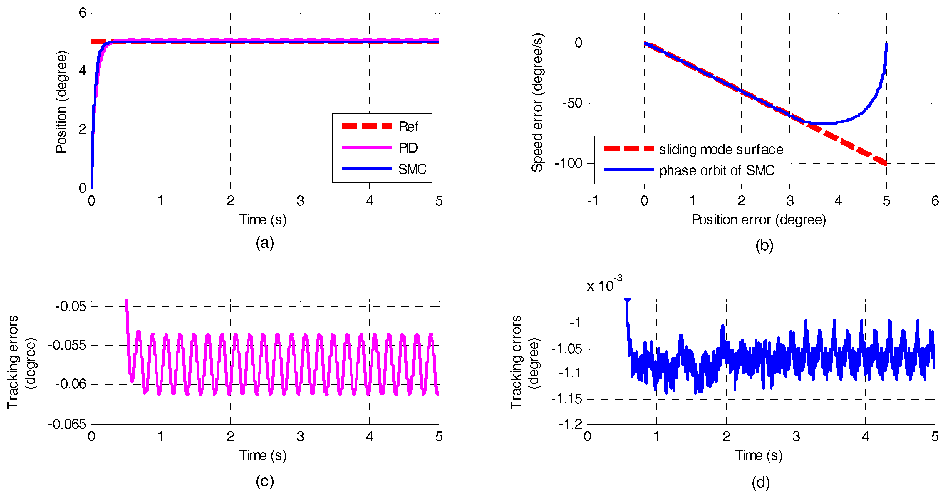
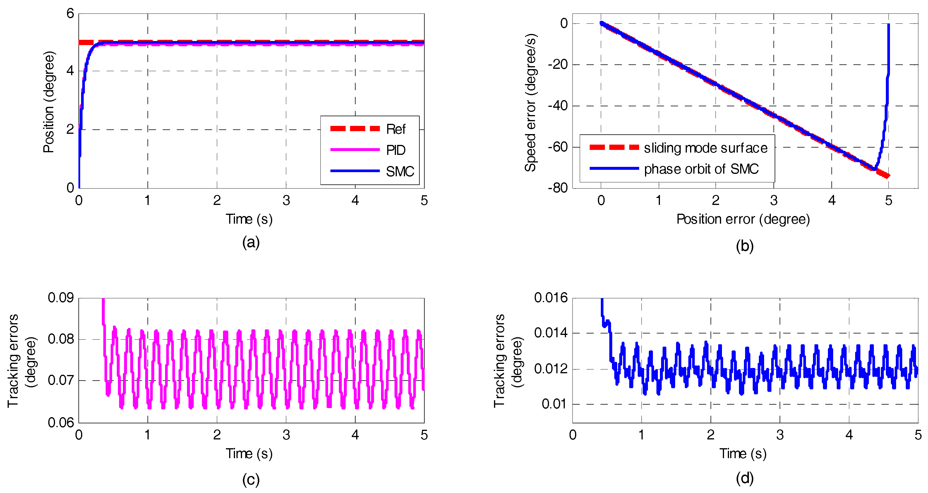
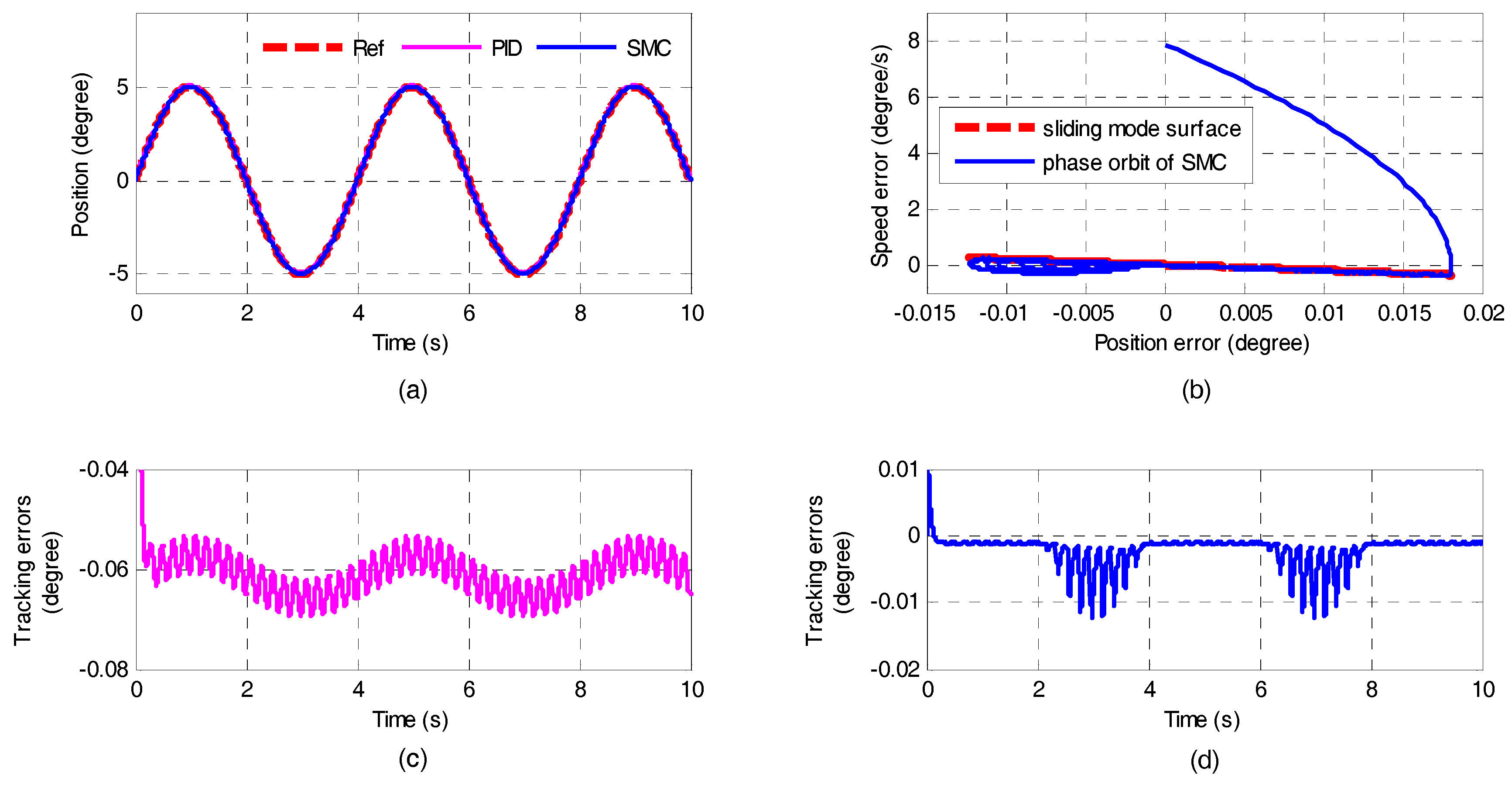
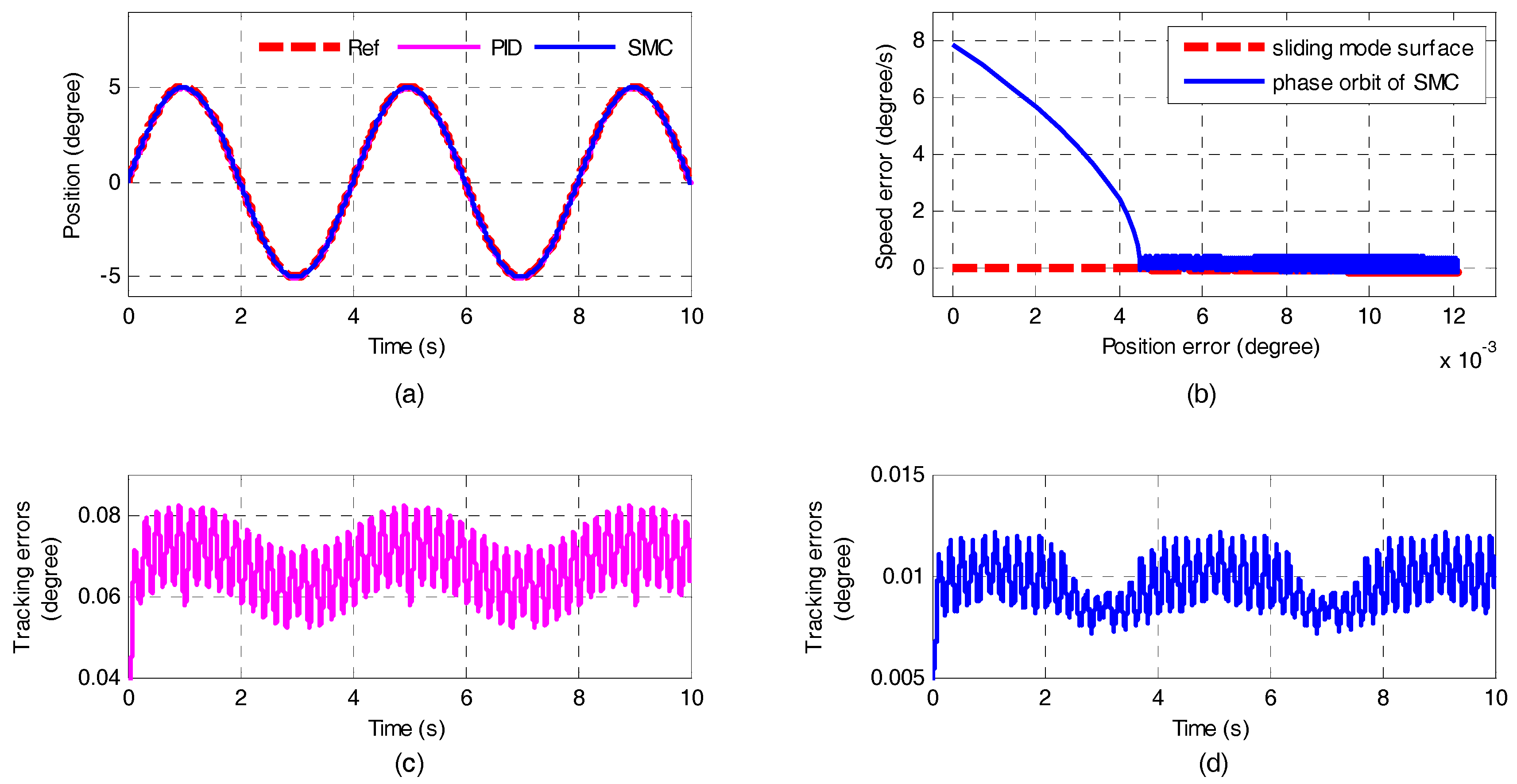
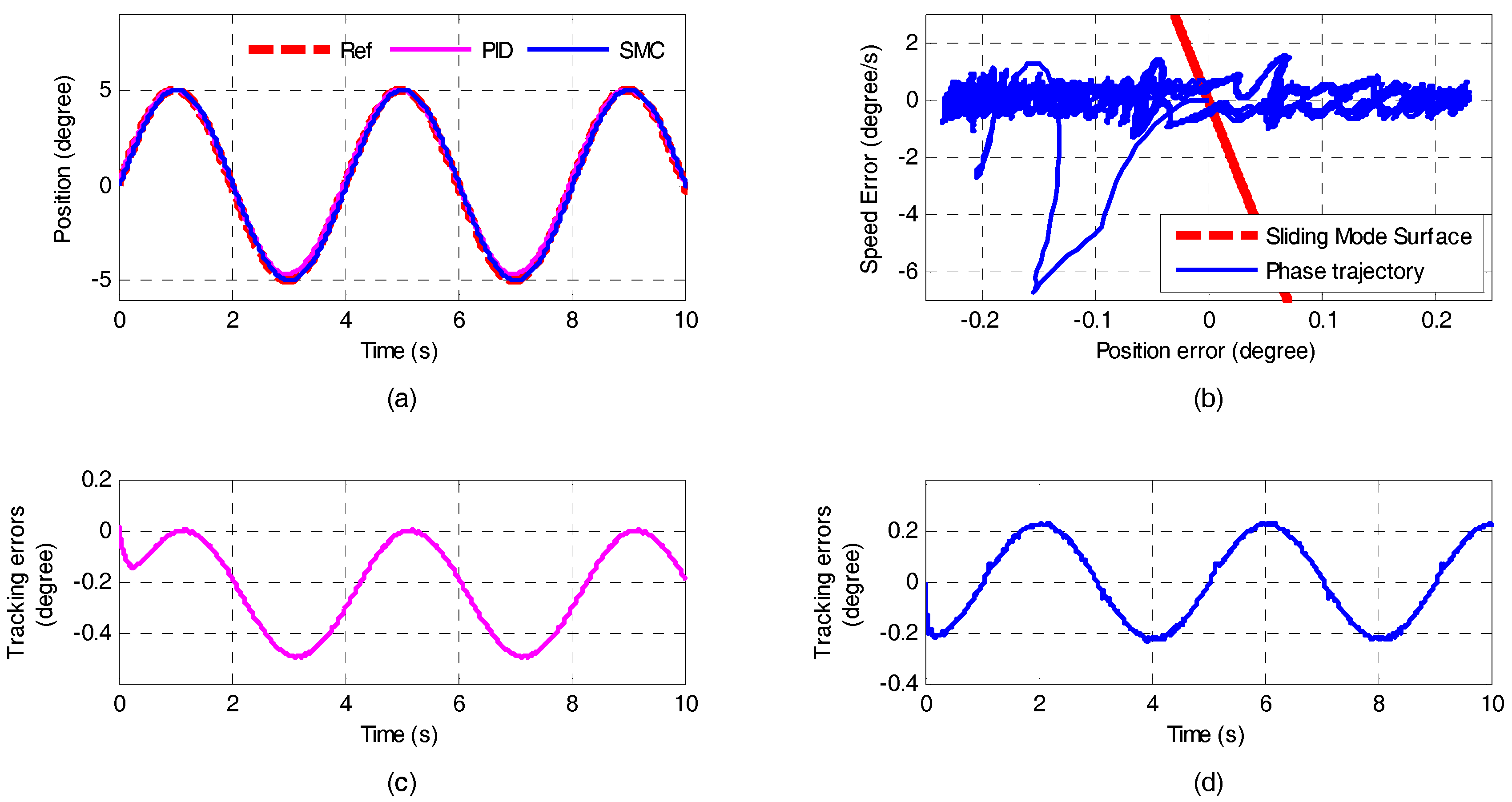
4.1. Simulations Results and Discussion

The parameters of the sliding mode controller (SMC) are selected as C = diag(20, 30), ε = diag(10, 20), and K = diag(20, 60). Set the disturbing torques of Joints 1 and 2, respectively, as ${\tau }_{d1}=0.5\sin \left(10\pi t\right)$ and ${\tau }_{d2}=0.5\cos \left(10\pi t\right)$.

The parameters of the Stribeck friction model are selected as listed in

Table 2. Parameters of the Stribeck friction model.

α	0.01
a1	1
Fs1	0.1 N·m
Fs2	0.05 N·m
Fc1	0.04 N·m
Fc2	0.02 N·m
Kv1	0.02
Kv2	0.01

.

The simulation results of the control law of sliding mode controller expressed by Equation (38) with the above parameters on step input are shown in Figure 4 and Figure 5 and on sinusoid input are shown in Figure 6 and Figure 7. A classical PID (proportional-integral-derivative) controller was also designed for comparison. The values of proportional, integral, and derivative gains of Joint 1 were P₁ = 102, I₁ = 1.2, and D₁ = 21.5, and the control parameters of Joint 2 were P₂ = 87, I₂ = 0.7, and D₂ = 15. These values have been optimally tuned using a modified Ziegler–Nichols’ (Z-N) tuning methods [31].

Figure 4 shows the step responses of Joint 1 with the proposed SMC and the PID controller. Figure 4a shows the position tracking with PID controller and the SMC. Figure 4b shows the phase trajectory diagram of the SMC. Figure 4c,d shows the tracking error with PID controller and the SMC, respectively. Figure 5 shows the step responses of Joint 2.

For step input, the adjusting times of both joints with the proposed SMC and the PID controller are only 0.2 s. However, the position steady state error of each joint with the SMC is far less than that with the PID controller. As shown in Figure 4c,d and Figure 5c,d, the tracking errors generated by the PID controller oscillate more intensely than that by the SMC. This phenomenon implies that the SMC possess better control accuracy and stronger robustness under disturbances than the PID. The phase trajectory of the SMC rapidly reaches the sliding mode surface from the initial point and quickly converges along the sliding mode surface to the equilibrium point. This illustrates that the designed SMC has good dynamic quality and uniform stability.

Figure 6 shows the sinusoidal responses of Joint 1 with the proposed SMC and the PID controller. Figure 6a shows the position tracking with PID controller and the SMC. Figure 6b shows the phase trajectory diagram of the SMC. Figure 6c,d shows the tracking error with PID controller and the SMC, respectively. Figure 7 shows the sinusoidal responses of Joint 2.

For sinusoidal input, as show in Figure 6 and Figure 7, an obvious lag or steady error is presented in the trajectory produced by the PID controller, which suffers from some difficulties in obtaining accurate tracking. The position tracking error of each joint with the PID controller oscillates more greatly than that with the SMC. The existence of this phenomenon suggests again that the SMC has better dynamic and static characteristic than the PID, and has high accuracy and stronger robustness. As shown in Figure 6b and Figure 7b, the phase trajectory rapidly reaches the sliding mode surface and quickly tends along the sliding mode surface to a tiny stable limit cycles around the equilibrium point. This illustrates that the designed sliding mode variable control has bounded stability. And the existence of the limit cycle implicates that the system has small steady state error.

The simulation results show that the influences of the friction torque and disturbances of the load torque and inertia are effectively suppressed by sliding mode variable structure control which has a strong adaptive ability to input signals.

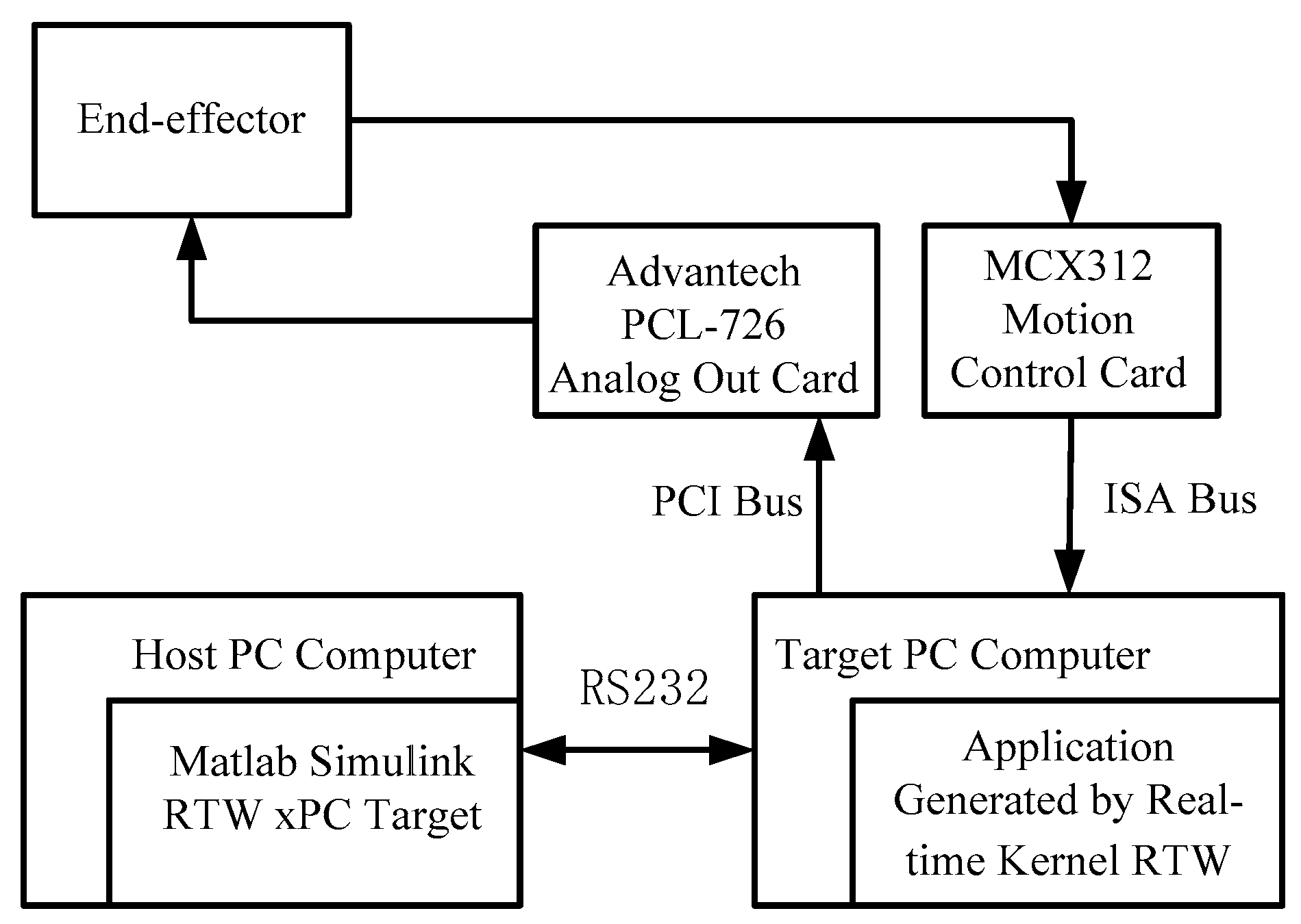
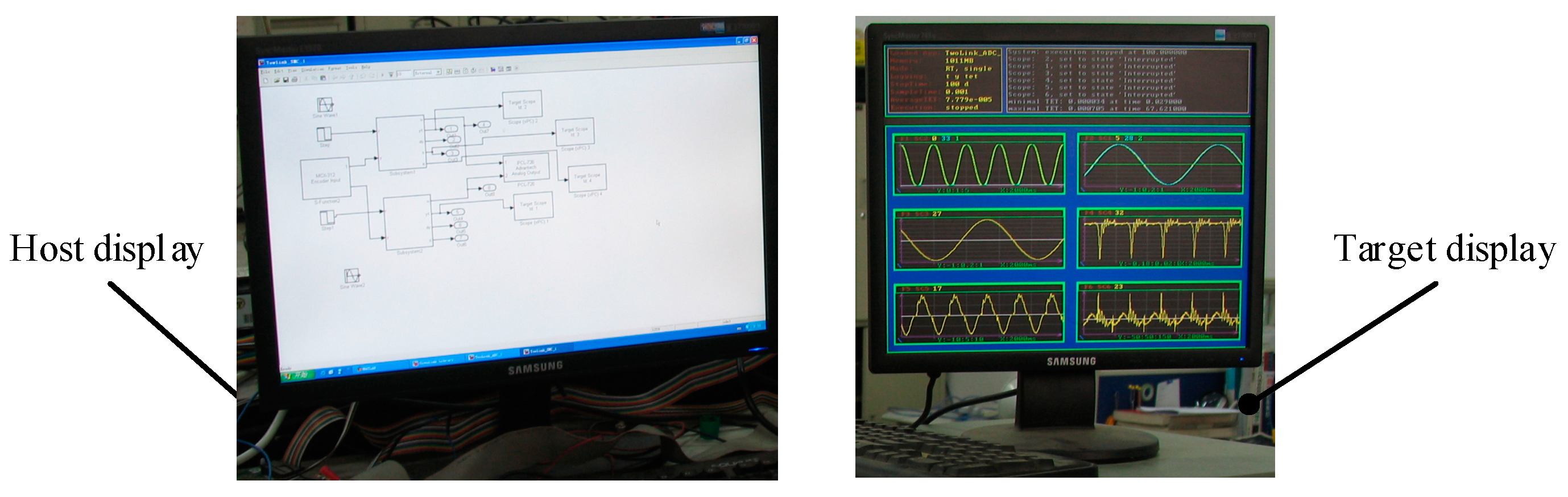
4.2. Establishment of Real-Time Experiment Platform

The key to validation of the dynamical model and the designed controller is to establish a reliable real time control system which has the characteristics of rapid response speed, flexibility, and low hardware cost. MATLAB provides a real-time development environment to achieve system simulation and product rapid-prototype by adopting the RTW (Real-Time Workshop) toolbox. RTW can automatically transform the model into dynamic system model code running on the hardware to realize real-time simulation and control.

xPC target environment adopts the Host-Target pattern. The Host is used for running Simulink model, compiling and generating executable code and then downloading it to the Target, it can also monitor and control the Target. The target is used for running executable code by installing highly optimized real-time kernel of 32-bit protected mode. The Host communicates with the Target using RS232 serial port or ethernet [32,33]. The real-time control experiment platform based on RTW xPC target environment is shown in Figure 8.

In the experiment, an Advantech PCL-726 analog output card is used for output of the control signal, and an MCX312 motion control card is used for collecting the position signal from the encoder. PLC-726 can be directly driven by the corresponding module in the I/O module library of xPC target. MCX312 isn’t included in the module library and its driver must be written. In the target system, the device driver must be written using C MEX S function which is a kind of S function written using C. Figure 9 shows the display of the RTW real-time experiment platform.

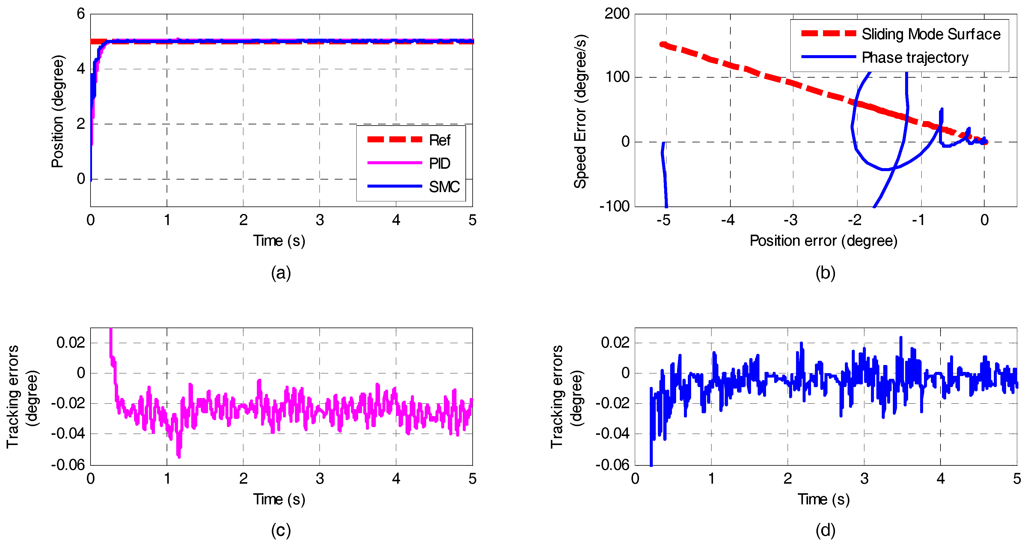
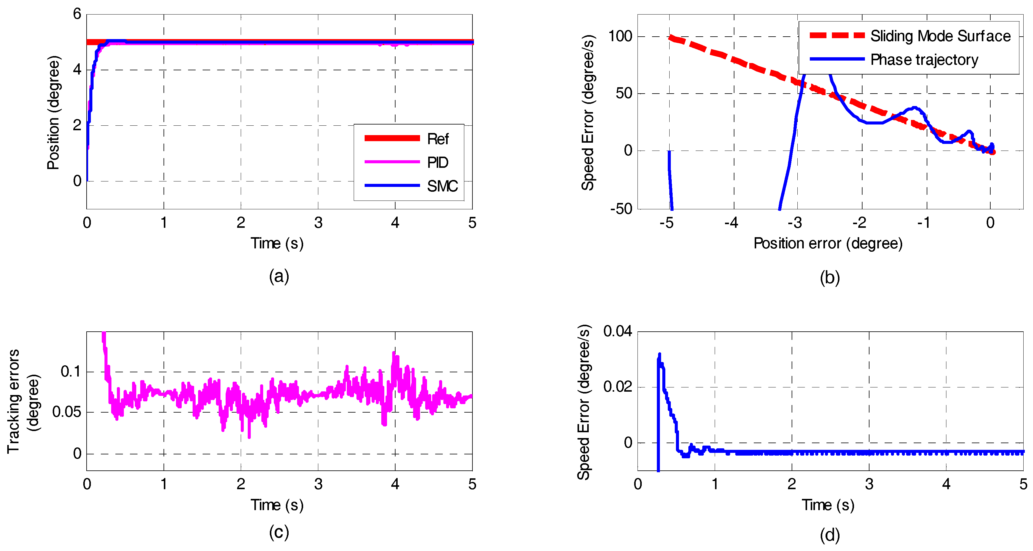
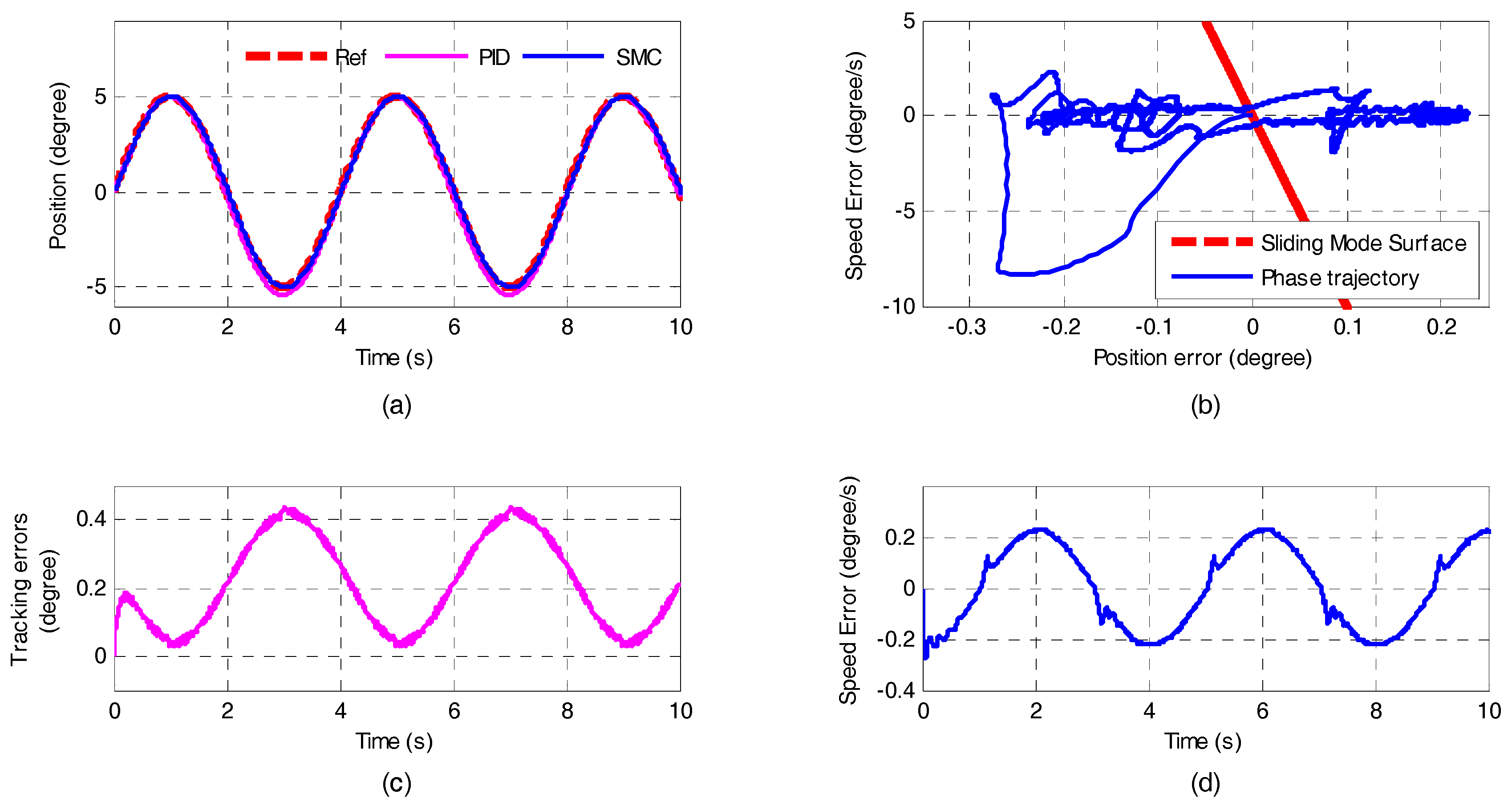
4.3. Experiments Results and Discussion

The symbolic function in the variable structure control expressed by Equation (38) is replaced by the saturation function to design quasi-sliding mode controller for reducing the chattering which is brought naturally by the sliding mode variable structure control in the experimental system. The new control law is expressed as:

$$u=C\dot{e}+{\ddot{q}}_d+\mathsf{\epsilon }sat\left(S\right)+KS$$

(43)

with

$$sat(s)=\{\begin{array}{lll}1\hfill & s>\Delta \hfill & \hfill \\ ks\hfill & \left|s\right|\le \Delta \hfill & k=\frac{1}{\Delta }\hfill \\ -1\hfill & s<-\Delta \hfill & \hfill \end{array}$$

(44)

where ∆ is the boundary layer, and ∆ = 0.05.

Experiments are carried out with the PID and the SMC controller respectively by applying a five-degree step input and a sinusoid input r = 5sin(0.5πt) to both of the Joints 1 and 2 in the same time. Figure 10 and Figure 11 show the step responses of the Joints 1 and 2, respectively. Figure 12 and Figure 13 show the sinusoid responses of the Joints 1 and 2, respectively.

For step input, as shown in Figure 10a and Figure 11a, the adjusting times of both joints with the proposed SMC and the PID controller are almost the same. However, the position steady state error of each joint with the SMC is far less than that with the PID controller, which is similar to the simulation results. As shown in Figure 10c,d, and Figure 11c,d, the tracking errors produced by the PID controller has higher oscillation amplitude than that by the SMC. This means that the SMC is more robust and accurate than the PID. As show in Figure 10b and Figure 11b, both of the phase trajectories of the SMC converge to stable limit cycles, this implicates that the system yields bounded stability based on sliding mode variable structure control. In order to accelerate the trajectory reaching to the sliding mode surface and improve the system dynamic quality during the experiment, the values of the parameter C of the switch function and the proportional gain K are set bigger. This causes in initial response that the phase trajectory generates obvious chatter along the sliding mode surface.

For sinusoid input, as show in Figure 12 and Figure 13, the position tracking experiment results of both of the Joints 1 and 2 with PID controller have obvious lag in contrast to that with the SMC, which suggests that the system with the SMC has higher tracking accuracy than that with the PID controller.

As shown in Figure 12b and Figure 13b, both of the phase trajectories converge to limit cycles around the equilibrium point, this implicates that the system based on the SMC gains bounded stability and has certain steady state errors. For the reason, the x-axis and y-axis have different coordinate ranges, both of the limit cycles look tabular. Actually, if the x-axis and y-axis have the same ranges, both of the limit cycles will appear more slim, which implicates that the speed errors are larger than the position errors.

5. Conclusions

In robotic control systems, nonlinearity and disturbances such as friction and differential signal may severely limit the performance of control. In this paper, a sliding mode variable structure control architecture is proposed for the normal adjustment of a designed robotic drilling end-effector. By using computation torque control and by adopting a third-order nonlinear integration chain differentiator for obtaining the speed and acceleration signals from the position signals, this sliding mode control scheme is developed with good dynamic quality. The new control law ensures global stability of the entire system and achieves both stabilization and tracking within a desired precision. A real-time control experiment platform is developed in xPC target environment based on MATLAB RTW to verify the proposed control scheme and simulation results. The experimental results prove that the proposed sliding mode control strategy is effective and robust with regard to external disturbances. The proposed controller is successfully tested on the normal adjustment of the robotic drilling end-effector. This research provides a solution for the more accurate control of robotic drilling on the curved surface of an airplane.

References

1. Wilson, M. Robots in the aerospace industry. Aircr. Eng. Aerosp. Technol. 1994, 66, 2–3. [Google Scholar] [CrossRef]
2. Cirillo, P.; Marino, A.; Natale, A.; Marino, E.D.; Chiacchio, P.; Maria, G.D. A low-cost and flexible solution for one-shot cooperative robotic drilling of aeronautic stack materials. IFAC-PapersOnLine 2017, 50, 4602–4609. [Google Scholar] [CrossRef]
3. Olsson, T.; Haage, M.; Kihlman, H.; Johansson, R.; Nilsson, K.; Robertsson, A.; Björkmsn, M.; Isaksson, R.; Ossbahr, G.; Brogårdh, T. Cost-efficient drilling using industrial robots with high-bandwidth force feedback. Rob. Comput. Integr. Manuf. 2010, 26, 24–38. [Google Scholar] [CrossRef]
4. Schneider, U.; Drust, M.; Ansloni, M.; Lehmann, C.; Pellicciari, M.; Leali, F.; Gunnink, J.W.; Verl, A. Improving robotic machining accuracy through experimental error investigation and modular compensation. Int. J. Adv. Manuf. Technol. 2016, 85, 3–15. [Google Scholar] [CrossRef] [Green Version]
5. Shi, Z.; Yuan, P.; Wang, Q.; Chen, D.; Wang, T. New design of a compact aero-robotic drilling end effector: An experimental analysis. Chin. J. Aeronaut. 2016, 29, 1132–1141. [Google Scholar] [CrossRef]
6. DeVlieg, R.; Sitton, K.; Feikert, E.; Inman, J. ONCE (one-sided cell end effector) robotic drilling system. SAE Tech. Pap. 2002. [Google Scholar] [CrossRef]
7. Atkinson, J.; Hartmann, J.; Jones, S.; Gleeson, P. Robotic drilling system for 737 aileron. SAE Tech. Pap. 2007. [Google Scholar] [CrossRef]
8. Webb, P.; Chitiu, A.; Fayad, C.; Gindy, N.; Mckeown, C. Flexible automated riveting of fuselage skin panels. SAE Trans. 2001, 110, 218–221. [Google Scholar]
9. Hempstead, B.; DeVlieg, R.; Mistry, R.; Sheridan, M. Drill and drive end effector. SAE Tech. Pap. 2001. [Google Scholar] [CrossRef]
10. Liang, J.; Bi, S. Design and experimental study of an end effector for robotic drilling. Int. J. Adv. Manuf. Technol. 2010, 50, 399–408. [Google Scholar] [CrossRef]
11. Devlieg, R. High-accuracy robotic drilling/milling of 737 inboard flaps. SAE Int. J. Aerosp. 2011, 4, 1373–1379. [Google Scholar] [CrossRef]
12. Gray, T.; Orf, D.; Adams, G. Mobile automated robotic drilling, inspection, and fastening. SAE Tech. Pap. 2013. [Google Scholar] [CrossRef]
13. Olsson, T.; Robertsson, A.; Johansson, R. Flexible force control for accurate low-cost robot drilling. In Proceedings of the 2007 IEEE International Conference on Robotics and Automation, Roma, Italy, 10–14 April 2007; IEEE: New York, NY, USA, 2007. [Google Scholar]
14. Tian, W.; Zhou, W.; Zhou, W.; Liao, W.; Zeng, Y. Auto-normalization algorithm for robotic precision drilling system in aircraft component assembly. Chin. J. Aeronaut. 2013, 26, 495–500. [Google Scholar] [CrossRef]
15. Mei, B.; Zhu, W.; Yuan, K.; Ke, Y. Robot base frame calibration with a 2D vision system for mobile robotic drilling. Int. J. Adv. Manuf. Technol. 2015, 80, 1903–1917. [Google Scholar] [CrossRef]
16. Frommknecht, A.; Kuehnle, J.; Effenberger, I.; Pidan, S. Multi-sensor measurement system for robotic drilling. Rob. Comput. Integr. Manuf. 2017, 47, 4–10. [Google Scholar] [CrossRef]
17. Qin, C.; Tao, J.; Wang, M.; Liu, C. A Novel Approach for the Acquisition of Vibration Signals of the End Effector in Robotic Drilling. In Proceedings of the 2016 IEEE International Conference on Aircraft Utility Systems (AUS), Beijing, China, 10–12 October 2016; IEEE: New York, NY, USA, 2016. [Google Scholar]
18. Garnier, S.; Subrin, K.; Waiyagan, K. Modelling of robotic drilling. Procedia CIRP 2017, 58, 416–421. [Google Scholar] [CrossRef]
19. Zhang, L.; Wang, X. A novel algorithm of normal attitude regulation for the designed end-effector of a flexible drilling robot. J. Southeast Univ. 2012, 28, 29–34. [Google Scholar]
20. Olsson, H.; Åström, K.J.; Wit, C.C.D.; Gäfvert, M.; Lischinsky, P. Friction models and friction compensation. Eur. J. Control 1998, 4, 176–195. [Google Scholar] [CrossRef]
21. Hung, J.Y.; Gao, W.; Hung, J.C. Variable structure control: A survey. IEEE Trans. Ind. Electron. 1993, 40, 2–22. [Google Scholar] [CrossRef]
22. Wang, X.; Liu, J.; Cai, K. Tracking control for a velocity-sensorless VTOL aircraft with delayed outputs. Automatica 2009, 45, 2876–2882. [Google Scholar] [CrossRef]
23. Karafyllis, I.; Kravaris, C. On the observer problem for discrete-time control systems. IEEE Trans. Ind. Electron. 2007, 52, 12–25. [Google Scholar] [CrossRef]
24. Drakunov, S.; Utkin, V. Sliding Mode Observers Tutorial. In Proceedings of the 34th IEEE Conference on Decision and Control, New Orleans, LA, USA, 13–15 December 1995; IEEE: New York, NY, USA, 1995. [Google Scholar]
25. Ma, R.; Zhang, G.; Krause, O. Fast terminal sliding-mode finite-time tracking control with differential evolution optimization algorithm using integral chain differentiator in uncertain nonlinear systems. Int. J. Robust Nonlinear Control 2018, 28, 625–639. [Google Scholar] [CrossRef]
26. Vasiljevic, L.; Khalil, H. Differentiation with High-Gain Observers the Presence of Measurement Noise. In Proceedings of the 45th IEEE Conference on Decision and Control, San Diego, CA, USA, 13–15 December 2006; IEEE: New York, NY, USA, 2007. [Google Scholar]
27. Alwi, H.; Edwards, C. An adaptive sliding mode differentiator for actuator oscillatory failure case reconstruction. Automatica 2013, 49, 642–651. [Google Scholar] [CrossRef] [Green Version]
28. Wang, X.; Lin, H. Design and analysis of a continuous hybrid differentiator. IET Control Theory Appl. 2011, 5, 1321–1334. [Google Scholar] [CrossRef] [Green Version]
29. Listmann, K.D.; Zhao, Z. A Comparison of Methods for Higher-Order Numerical Differentiation. In Proceedings of the 2013 European Control Conference (ECC), Zurich, Switzerland, 17–19 July 2013; IEEE: New York, NY, USA, 2013. [Google Scholar]
30. Wang, X.; Chen, Z.; Yuan, Z. Design and analysis for new discrete tracking-differentiators. Appl. Math. A J. Chin. Univ. 2003, 18, 214–222. [Google Scholar] [CrossRef]
31. Meshram, P.M.; Kanojiya, R.G. Tuning of PID Controller Using Ziegler-Nichols Method for Speed Control of DC Motor. In Proceedings of the IEEE-International Conference on Advances in Engineering, Science and Management (ICAESM-2012), Nagapattinam, Tamil Nadu, India, 30–31 March 2012; IEEE: New York, NY, USA, 2012. [Google Scholar]
32. Low, K.H.; Wang, H.; Wang, M.Y. On the Development of a Real Time Control System by Using xPC Target: Solution to Robotic System Control. In Proceedings of the IEEE International Conference on Automation Science and Engineering, Edmonton, AB, Canada, 1–2 August 2005; IEEE: New York, NY, USA, 2005. [Google Scholar]
33. Grepl, R. Real-Time Control Prototyping in MATLAB/Simulink: Review of Tools for Research and Education in Mechatronics. In Proceedings of the 2011 IEEE International Conference on Mechatronics, Istanbul, Turkey, 13–15 April 2011; IEEE: New York, NY, USA, 2011. [Google Scholar]
Figure 1. Structure and prototype of the designed end-effector: (a) the diagram of the end-effector structure; (b) the specific of the internal structure of the end-effector; and (c) the prototype of the end-effector.
Applsci 08 01892 g001
Figure 2. Coordination definition of the end-effector.
Applsci 08 01892 g002
Figure 3. The sliding mode variable structure control block diagram.
Applsci 08 01892 g003
Figure 4. Simulation of step response of Joint 1: (a) Position tracking; (b) Phases trajectory diagram of SMC; (c) Tracking error of PID (proportional-integral-derivative); and (d) Tracking error of SMC (sliding mode controller).
Applsci 08 01892 g004
Figure 5. Simulation of step response of Joint 2: (a) Position tracking; (b) Phases trajectory diagram of SMC; (c) Tracking error of PID; and (d) Tracking error of SMC.
Applsci 08 01892 g005
Figure 6. Simulation of sinusoidal response of Joint 1: (a) Position tracking; (b) Phases trajectory diagram of SMC; (c) Tracking error of PID; and (d) Tracking error of SMC.
Applsci 08 01892 g006
Figure 7. Simulation of sinusoidal response of Joint 2: (a) Position tracking; (b) Phases trajectory diagram of SMC; (c) Tracking error of PID; and (d) Tracking error of SMC.
Applsci 08 01892 g007
Figure 8. Real-Time Workshop (RT W) xPC target real-time control platform principle diagram.
Applsci 08 01892 g008
Figure 9. The display of the RTW real-time experiment platform.
Applsci 08 01892 g009
Figure 10. Experiment of step response of Joint 1: (a) Position tracking; (b) Phases trajectory diagram of SMC; (c) Tracking error of PID; and (d) Tracking error of SMC.
Applsci 08 01892 g010
Figure 11. Experiment of step response of Joint 2: (a) Position tracking; (b) Phases trajectory diagram of SMC; (c) Tracking error of PID; and (d) Tracking error of SMC.
Applsci 08 01892 g011
Figure 12. Experiment of sinusoidal response of Joint 1: (a) Position tracking; (b) Phases trajectory diagram of SMC; (c) Tracking error of PID; and (d) Tracking error of SMC.
Applsci 08 01892 g012
Figure 13. Experiment of sinusoidal response of Joint 2: (a) Position tracking; (b) Phases trajectory diagram of SMC; (c) Tracking error of PID; and (d) Tracking error of SMC.
Applsci 08 01892 g013