Article

Sliding Mode Thau Observer for Actuator Fault Diagnosis of Quadcopter UAVs

Faculty of Mechanical and Aerospace Engineering, Sejong University, Seoul 05006, Korea
*
Author to whom correspondence should be addressed.
Appl. Sci. 2018, 8(10), 1893; https://doi.org/10.3390/app8101893
Submission received: 6 September 2018 / Revised: 2 October 2018 / Accepted: 2 October 2018 / Published: 11 October 2018
(This article belongs to the Special Issue Advanced Mobile Robotics)

Abstract

:

Featured Application

This work addresses issues related to fault-tolerant control of quadcopter UAVs.

Abstract

Fault diagnosis (FD) is one of the main roles of fault-tolerant control (FTC) systems. An FD should not only identify the presence of a fault, but also quantify its magnitude and location. In this work, we present a robust fault diagnosis method for quadcopter unmanned aerial vehicle (UAV) actuator faults. The state equation of the quadcopter UAV is examined as a nonlinear system. An adaptive sliding mode Thau observer (ASMTO) method is proposed to estimate the fault magnitude through an adaptive algorithm. We then obtain the design matrices and parameters using the linear matrix inequalities (LMI) technique. Finally, experimental results are presented to show the advantages of the proposed algorithm. Unlike previous research on quadcopter UAV FD systems, our study is based on ASMTO and can, therefore, determine the time variability of a fault in the presence of external disturbances.

1. Introduction

Quadcopter unmanned aerial vehicles (UAVs) have been used in a variety of applications, due to their numerous advantages, such as small size, agility, low cost, mechanical simplicity, and indoor and outdoor operability, which have led to their increased popularity compared to other UAV systems. As a result, they have been investigated and tested in a range of environments and applications which include target tracking [1,2], fault detection and fault-tolerant control [3,4], and formation flight [5,6].
Particularly the topic of fault-tolerant control (FTC) has received a large amount of attention in the community, which led to quadcopter UAVs that are less error-prone and, thus, more reliable during flight. In general, there are two types of FTC: passive and active. Several studies investigated passive FTCs [7,8], which have the advantage that they do not require any fault diagnosis scheme, but the resulting disadvantage is that they have a lower fault tolerance [9]. To overcome this limitation, active FTCs have been introduced to improve said fault tolerance. Fault diagnosis (FD) is the essential requirement for active FTCs to determine the location and magnitude of faults. Through FD, active FTCs can be designed to compensate the effect of faults and, thus, improve flight control and stability, which makes FD the main task of active FTCs.
The FD approach has been studied by numerous authors. Freddi et al. [10,11] investigated a model-based fault diagnosis which can be used to monitor sensor faults and detect actuator faults. In this method, residuals are used to distinguish between system and observer outputs, but these methods are inaccurate and unsuitable for quantifying the magnitude of a fault. Ma and Zhang [12,13] proposed a method for fault estimation based on a Kalman filter, but their approach is of insufficient robustness with regard to disturbances if the transfer matrices are inaccurate. Several effective approaches, such as sliding mode observer [14,15], neural network [16,17], and adaptive observer [18,19], have been investigated, but none of these approaches focused on a real quadcopter UAV. Moreover, recent studies [20,21] used fuzzy methods for fault diagnosis problems, but these approaches do not focus on real quadcopters, and may be overly complex to implement in a flight controller. Only few studies focused on the problem of fault diagnosis in a real quadcopter UAV, verified through real flight data. While [4] used an actuator fault estimation with an adaptive observer based on H , and demonstrated the effectiveness of the proposed scheme, this method may not be sufficiently robust to external disturbances because the underlying mathematical model neglects both nonlinear terms and external disturbances. The most recent application of an adaptive Thau observer (ATO) for actuator fault diagnosis was proposed in [22]. While this approach is capable of handling model uncertainties in the nonlinear quadcopter model, it is rather complex and time-consuming because it uses system identification to find the drag terms, and the filter to eliminate sensor noise.
In the present study, we try to overcome these limitations by combining a sliding mode observer based on Walcott–Zak observer design [23], with ATO to handle the actuator fault diagnosis. This method is capable of accounting for time-varying actuator faults. We then derive the Lyapunov stability and other conditions to obtain the desired matrices and associated parameters. Finally, a straightforward method based on linear matrix inequalities (LMI) is proposed to allow relaxing the derived conditions, which is a useful feature in flight controllers. Unlike previous methods, our approach is simple and not overly time-consuming, which makes it amenable for use in real quadcopters. Moreover, our method can handle uncertainties of magnitudes that are unknown, a priori, through an adaptive law approach. By comparing our approach to [22], we found that the adaptive algorithm is capable of compensating for the drag terms leading to clear improvements in the results.

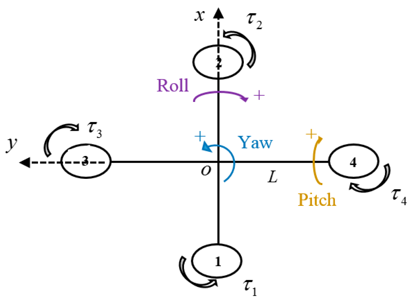
2. System Description

While the right and left (3 and 4) motors of the quadcopter rotate in the clockwise direction, the other motors rotate in counterclockwise direction (Figure 1). Each motor is located at a distance L from the center of mass o .
Assuming the control variables can be described as
{ U 1 = T 1 + T 2 + T 3 + T 4 U 2 = ( T 3 T 4 ) L U 3 = ( T 1 T 2 ) L U 4 = τ 1 + τ 2 τ 3 τ 4 ,
where τ i and T i represent the torque and thrust force produced by the i th motor, respectively; U 1 is the total thrust; U 2 ,   U 3 ,   U 4 are the torques in ϕ , θ , ψ directions, which correspond to roll, pitch, and yaw Euler angles, respectively (Figure 1).
Thrust force and torque are related to the rotational speed as follows:
T i = b Ω i 2 ,
τ i = d Ω i 2 ,
where b ,   d represent the thrust and drag coefficients, and Ω i represents the rotational speed of the i th motor.
Inserting Equations (2) and (3) into (1) yields
{ U 1 = b ( Ω 1 2 + Ω 2 2 + Ω 3 2 + Ω 4 2 ) U 2 = b ( Ω 3 2 Ω 4 2 ) U 3 = b ( Ω 1 2 Ω 2 2 ) U 4 = d ( Ω 1 2 + Ω 2 2 Ω 3 2 Ω 4 2 ) .
The quadcopter dynamic model has previously been formulated as follows [22,24]:
{ I x ϕ ¨ = U 2 + ( I y I z ) θ ˙ ψ ˙ J T θ ˙ Ω K ϕ ϕ ˙ I y θ ¨ = U 3 + ( I z I x ) ϕ ˙ ψ ˙ J T ϕ ˙ Ω K θ θ ˙ I z ψ ¨ = U 4 + ( I x I y ) ϕ ˙ θ ˙ K ψ ψ ˙ ,
where I x ,   I y ,   I z represent the moments of inertia along the x ,   y ,   z directions, respectively; K ϕ ,   K θ ,   K ψ are drag coefficients; J T is the moment of inertia of each motor, and Ω = Ω 3 + Ω 4 Ω 1 Ω 2 .
We consider drag terms as disturbances, and they can be compensated by adaptive law, which is discussed in the “nonlinear observer for fault diagnosis” section. By defining the state vector x T = [ ϕ θ ψ ϕ ˙ θ ˙ ψ ˙ ] , control input vector u T = [ U 2 U 3 U 4 ] , and output vector y T = [ ϕ θ ψ ϕ ˙ θ ˙ ψ ˙ ] , Equation (5) can be described in the state equation as
{ x ˙ ( t ) = A x ( t ) + p ( x , u ) + B u ( t ) + E d d ( t ) y = C x ( t ) ,
where E d is disturbance matrix, d ( t ) R s is disturbance vector, A = [ 0 0 0 1 0 0 0 0 0 0 1 0 0 0 0 0 0 1 0 0 0 0 0 0 0 0 0 0 0 0 0 0 0 0 0 0 ]   , B = [ 0 0 0 0 0 0 0 0 0 1 / I x 0 0 0 1 / I y 0 0 0 1 / I z ] , C = I 6 × 6 , and p ( x , u ) = [ 0 0 0 ( θ ˙ ψ ˙ ( I y I z ) J T θ ˙ Ω ) / I x ( ϕ ˙ ψ ˙ ( I z I x ) J T ϕ ˙ Ω ) / I y ϕ ˙ θ ˙ ( I x I y ) / I z ] . When an actuator fault occurs, Equation (6) can be described as
{ x ˙ ( t ) = A x ( t ) + p ( x , u ) + B u ( t ) + F f ( t ) + E d d ( t ) y = C x ( t ) ,
where F is the fault matrix, and f ( t ) R l is an actuator fault vector.

3. Nonlinear Observer for Fault Diagnosis

3.1. Standard Thau Observer for Fault Detection

According to the state Equation (7), the two following conditions must be met by the Thau observer design:
C1 the pair ( C ,   A ) is observable.
C2 the nonlinear term p ( x , u ) is continuously differentiable and assumed to be Lipschitz, with a constant γ , i.e., p ( x 1 ( t ) , u ( t ) ) p ( x 2 ( t ) , u ( t ) ) γ x 1 x 2 .
From the above conditions, the state Equation (7), based on Thau observer, can be constructed as [20]:
{ x ^ ˙ ( t ) = A x ^ ( t ) + p ( x ^ , u ) + B u ( t ) + K ( y ^ ( t ) y ( t ) ) y ^ = C x ^ ( t ) ,
where K is the observer gain matrix which is determined by
Lemma 1.
[11]: If the given observer gain matrix in Equation (8) satisfies
K = P ε 1 C T ,
then matrix P ε can be obtained from the Lyapunov equation
A T P ε + P ε A C T C + ε C T P ε = 0 ,
where ε is a positive constant such that P ε 0 , and the state space model Equation (6) is an asymptotic estimation with lim t e ( t ) = lim t ( x ^ ( t ) x ( t ) ) = 0 .

3.2. Adaptive Sliding Mode Thau Observer for Fault Diagnosis

The following conditions and lemmas are given for the ASMTO design:
C3 f ( t ) and   f ˙ ( t ) are norm-bounded, i.e., f ( t ) f 1 , f ˙ ( t ) f 2 , with f 1 , f 2 > 0.
C4 There exists an unknown constant that satisfies d ( t ) N .
Lemma 2.
For a given symmetric matrix P 0 and scalar μ > 0 , the following inequality must be satisfied:
2 x T y 1 μ x T P x + μ y T P 1 y .
Lemma 3.
If C2 holds, there exists a matrix P 0 such that
2 e T P ( p ( x 1 , u ) p ( x 2 , u ) ) γ 2 e T P P e + e T e .
If all the above conditions and lemmas hold, then the ASMTO has a form
{ x ^ ˙ ( t ) = A x ^ ( t ) + p ( x ^ , u ) + B u ( t ) + E d v ( t ) + F f ^ ( t )   + K ( y ^ ( t ) y ( t ) ) y ^ = C x ^ ( t ) ,
where x ^ ( t ) R n ,   f ^ ( t ) R l ,   y ^ ( t ) R q are the observer state vector, fault estimation of f ( t ) , and observer output vector, respectively. K is the Thau observer gain matrix and v ( t ) is given by the following algorithm:
n ˙ ( t ) = α F 1 e y ( t ) v ( t ) = n ( t ) F 1 e y ( t ) F 1 e y ( t ) ,
where α is a constant and F 1 is discussed in the “stability analysis” section.

3.3. Stability Analysis

Denote
e x = x ^ ( t ) x ( t ) n ˜ ( t ) = n ( t ) N e y = y ^ ( t ) y ( t ) e f = f ^ ( t ) f ( t ) .
Then, the error dynamics can be obtained from (7), (13), and (15) as
e ˙ x ( t ) = ( A K C ) e x + p ( x ^ , u ) p ( x , u ) + F e f + E d ( v ( t ) d ( t ) ) .
Theorem 1.
For a given observer gain, K , if there exist matrices P = P T > 0 ,   G = G T > 0 ,   F 1 , and F 2 such that
[ P ( A K C ) + ( A K C ) T P + γ 2 P P + I 0 0 σ + 1 σ G ] < 0 ,
E d T P = 1 σ F 1 C ,
F T P = 1 σ F 2 C ,
where σ is positive constant, then, the fault estimation algorithm can be described as
f ^ ˙ ( t ) = Γ F 2 e y + σ Γ f ^ ( t ) ,
where Γ is the learning rate matrix, Γ = Γ T > 0 .
Remark 1.
The adaptive law in Equation (20) uses both error dynamics and fault vector information. While the proportional term can lead to a rapid improvement in system response, the fault vector can eliminate the error of estimation.
Proof. 
Considering the following Lyapunov function.
V ( t ) = e x T P e x + 1 σ e f T Γ 1 e f + 1 σ n ˜ T α 1 n ˜
Then, its time derivative V ˙ ( t ) is
V ˙ ( t ) = e ˙ x T ( t ) P e x ( t ) + e x T ( t ) P e ˙ x ( t ) + 2 σ e f T ( t ) Γ 1 e ˙ f ( t ) + 2 σ n ˙ ( t ) α 1 n ˜ ( t ) = e x T ( t ) [ P ( A K C ) + ( A K C ) T P ] e x ( t ) + 2 e x T ( t ) P E d ( v ( t ) d ( t ) ) + 2 e x T ( t ) P F e f ( t ) + 2 σ F 1 e y ( t ) ( n ( t ) N ) + 2 e x T ( t ) P ( p ( x ^ , u ) p ( x , u ) ) + 2 σ e f T Γ 1 f ^ ˙ ( t ) 2 σ e f T Γ 1 f ˙ ( t ) .
Using Theorem 1, Lemma 2, and Lemma 3, one can see that
2 e x T ( t ) P F e f ( t ) + 2 σ e f T Γ 1 f ^ ˙ ( t ) = 2 e x T ( t ) P F e f ( t ) + 2 σ e f T Γ 1 ( Γ F 2 e y + σ Γ f ^ ( t ) ) = 2 e f T f ^ ( t ) e f T G e f + f ^ T ( t ) G 1 f ^ ( t ) e f T G e f + f 1 2 λ max ( G 1 ) ,
2 e x T ( t ) P E d ( v ( t ) d ( t ) ) = 2 σ ( F 1 e y ( t ) ) T ( n ( t ) F 1 e y ( t ) F 1 e y ( t ) d ( t ) ) < 2 σ F 1 e y ( t ) ( n ( t ) N ) ,
where λ max is the maximum eigenvalue of the associated matrix.
From Lemma 2, one can see that
2 σ e f T ( t ) Γ 1 f ˙ ( t ) = 2 σ ( e f T ( t ) ) ( Γ 1 f ˙ ( t ) ) 1 σ ( e f T ( t ) G e f ( t ) + f ˙ T ( t ) Γ 1 G 1 Γ 1 f ˙ ( t ) ) 1 σ ( e f T ( t ) G e f ( t ) + f 2 2 λ max ( Γ 1 G 1 Γ 1 ) ) .
According to Lemma 3, we obtain
e x T ( t ) [ P ( A K C ) + ( A K C ) T P ] e x ( t ) + 2 e x T ( t ) P ( p ( x ^ , u ) p ( x , u ) ) e x T ( t ) [ P ( A K C ) + ( A K C ) T P + γ 2 P P + I ] e x ( t ) .
With (23), (24), (25), and (26), Equation (22) becomes
V ˙ ( t ) = e x T ( t ) [ P ( A K C ) + ( A K C ) T P + γ 2 P P + I ] e x ( t ) + e f T G e f + f 1 2 λ max ( G 1 ) + 1 σ ( e f T ( t ) G e f ( t ) + f 2 2 λ max ( Γ 1 G 1 Γ 1 ) ) = e x T ( t ) [ P ( A K C ) + ( A K C ) T P +   γ 2 P P + I ] e x ( t ) σ + 1 σ e f T ( G ) e f + η ξ T ( t ) Θ ξ ( t ) + η ,
where η = f 1 2 λ max ( G 1 ) + 1 σ f 2 2 λ max ( Γ 1 G 1 Γ 1 ) ) , ξ ( t ) = [ e x T ( t ) e f T ( t ) ] , and Θ = [ P ( A K C ) + ( A K C ) T P + γ 2 P P + I 0 0 σ + 1 σ G ] .
If Θ < 0 , then V ˙ ( t ) < 0 for σ ξ ( t ) 2 > η , where σ = λ min ( Θ ) . This means that ( e x ( t ) , e y ( t ) ) converges to a small set, according to Lyapunov stability theory [25]. ☐
Remark 2.
It is difficult to solve Equations (17)–(19) simultaneously, and this problem can be addressed using the LMI technique. Therefore, we modify Equations (18) and (19) to [25]
[ η 1 I E d T P F 1 C ( E d T P F 1 C ) T η 1 I ] > 0 ,
[ η 2 I F T P 1 σ F 2 C ( F T P 1 σ F 2 C ) T η 2 I ] > 0 .

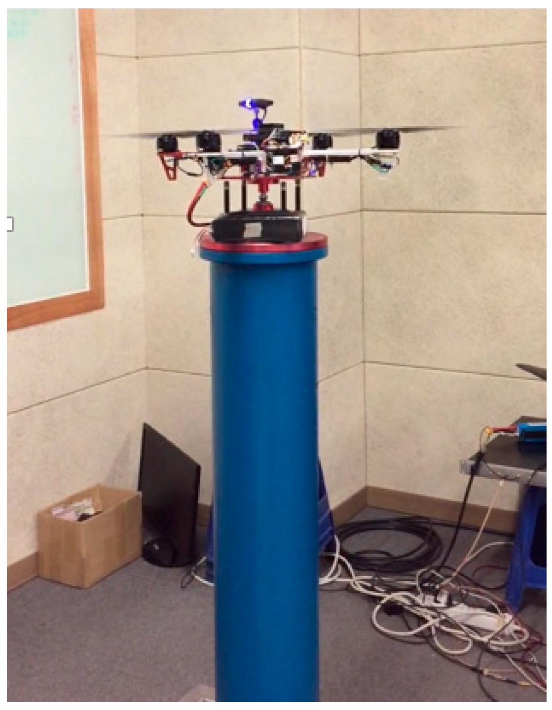
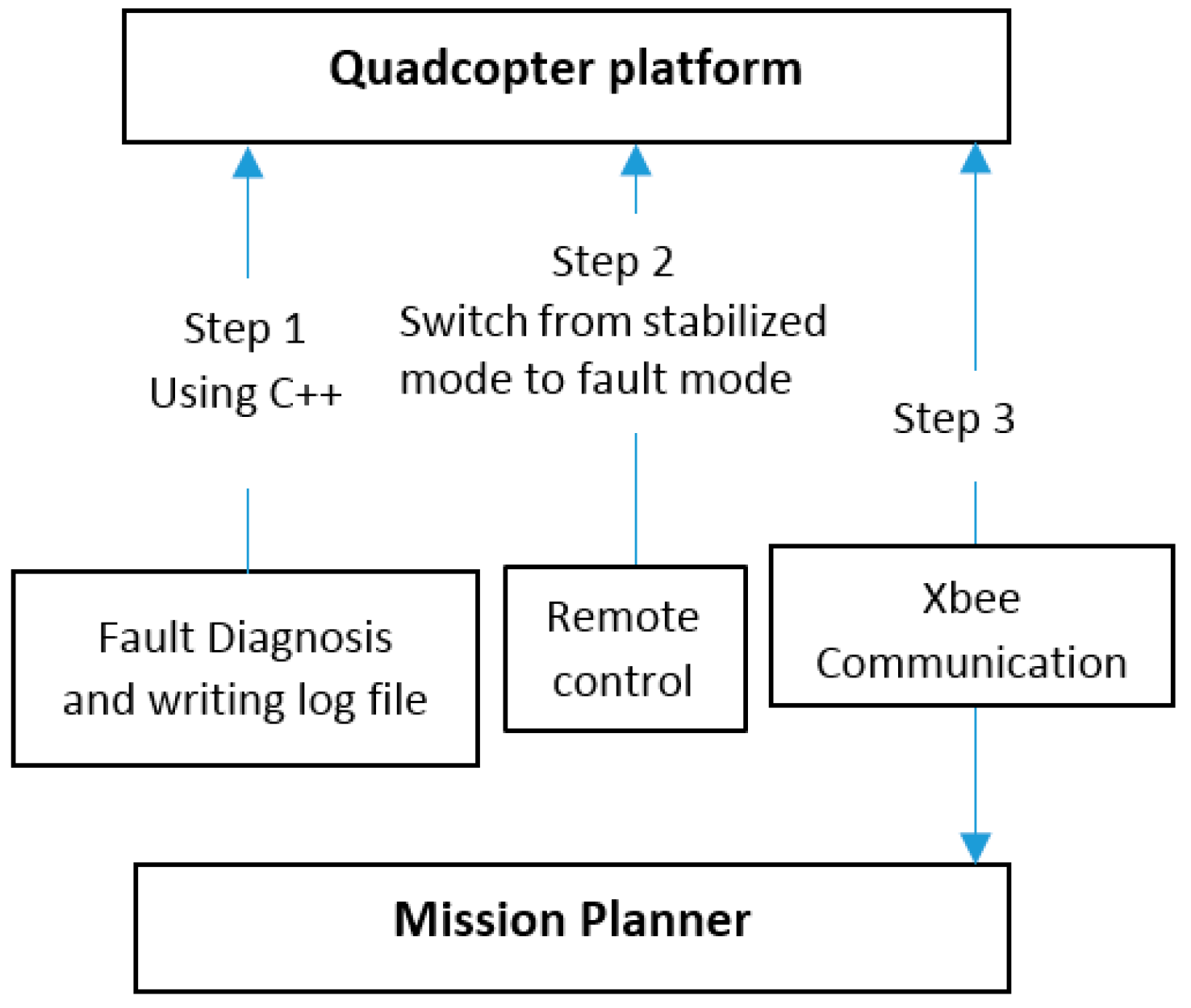
4. Experimental Results

4.1. Experimental Setup and Parameters

For safety purposes, the quadcopter test bed was developed in the guidance, navigation, and control (GNC) lab (Figure 2). The fault diagnosis algorithm from Section 3 was tested on a DJI F450 quadcopter. The algorithm was implemented on a Pixhawk2 flight controller using C++ program from Eclipse software [26]. The flight controller used firmware version 3.5. In the experimental setup, a remote control was used to inject faults by limiting the pulse width modulation (PWM) of the motors, which allowed us to switch between stabilized and fault modes. During testing, the Mission Planner (MP), a commercially available software, was used to monitor flight data through Xbee (Telemetry) communication [27]. Since the MP has some limitations with regard to parameter monitoring, the fault estimation data had to be obtained through a C++ program that writes them to a log file. The experimental procedure is summarized in Figure 3.
The DJI F450 parameter values are shown in Table 1. For the experiment, the matrices were chosen as follows: the fault matrix F = B , and the disturbance matrix E d = [ 1 1 1 1 1 1 ] T . The pair ( A , C ) is observable and condition C1 is satisfied, p ( x , u ) is continuously differentiable, and satisfies condition C2 as it only contains multiplications and divisions. Thus, all conditions are met, and the proposed scheme is applicable.
We used the following learning rate Γ = d i a g ( 0.005 , 0.005 , 0.005 ) and sampling time T = 0.0025   s for the experimental test bed. The matrices obtained from the ASMTO are F 1 = [ 101.77 101.77 101.77 101.77 101.77 101.77 ] ,   F 2 = [ 26 5 5 13 , 946 5 5 5 24 5 5 12 , 887 5 3 3 16 3 3 8701 ] G = 100 × I 6 × 6 ,   K = [ 100 0 0 1 0 0 0 100 0 0 1 0 0 0 100 0 0 1 1 0 0 100 0 0 0 1 0 0 100 0 0 0 1 0 0 100 ] ,   P = [ 101.8 0.04 0.04 0.19 0.04 0.04 0.04 101.81 0.04 0.04 0.19 0.04 0.04 0.04 101.8 0.04 0.04 0.19 0.19 0.04 0.04 101.8 0.04 0.04 0.04 0.19 0.04 0.04 101.8 0.04 0.04 0.04 0.19 0.04 0.04 101.8 ] .
The 30% partial loss fault is injected artificially into motor 1 by limiting the PWM of the motor at time t = 7 s. This is achieved by changing from stabilized mode to fault mode using the remote control. The fault percentage is user-controllable, and can be set in the C++ program. The moments of motors M2, M3, and M4 remained zero while the moment of motor M1 decreases because of the actuator fault (Figure 4).

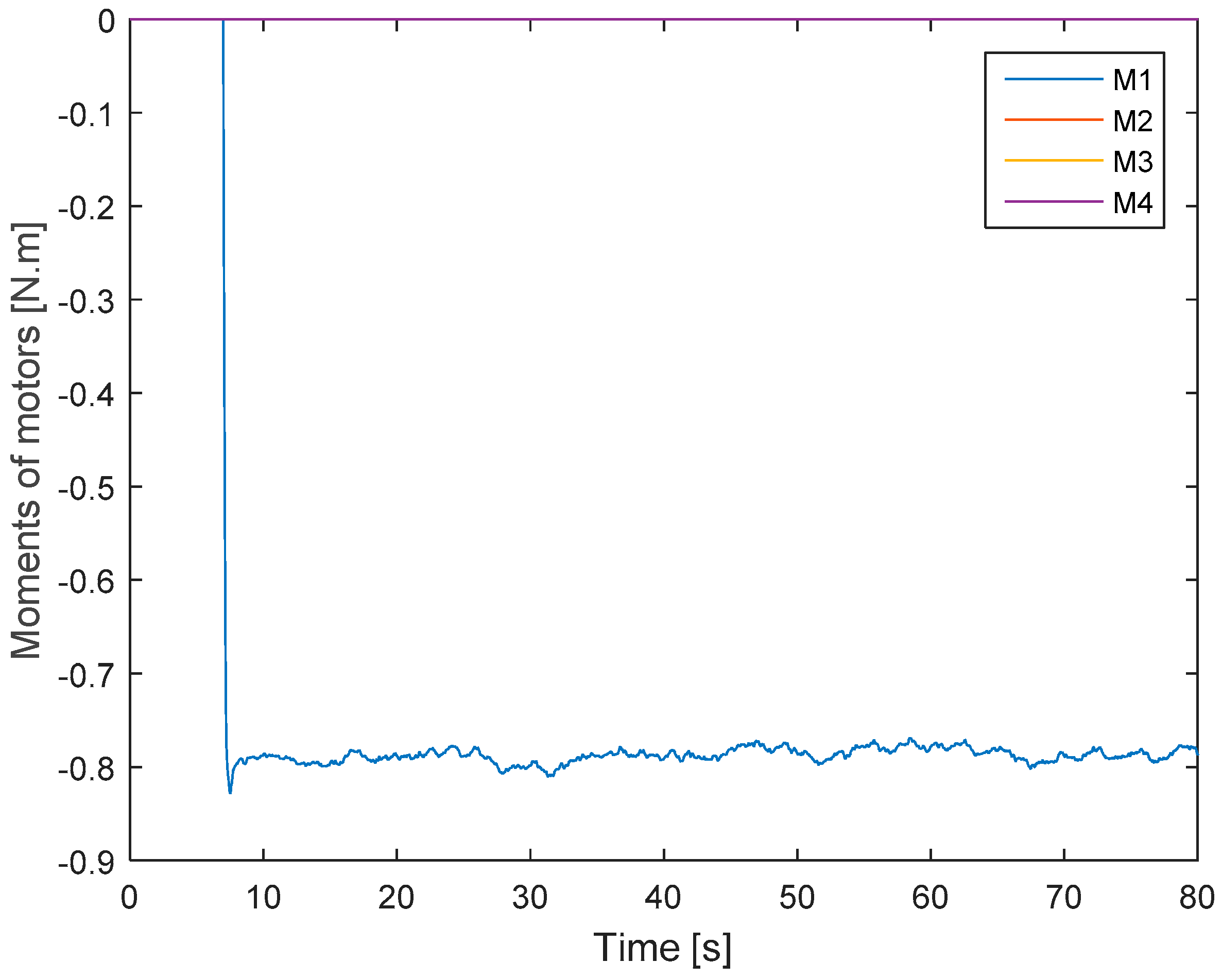
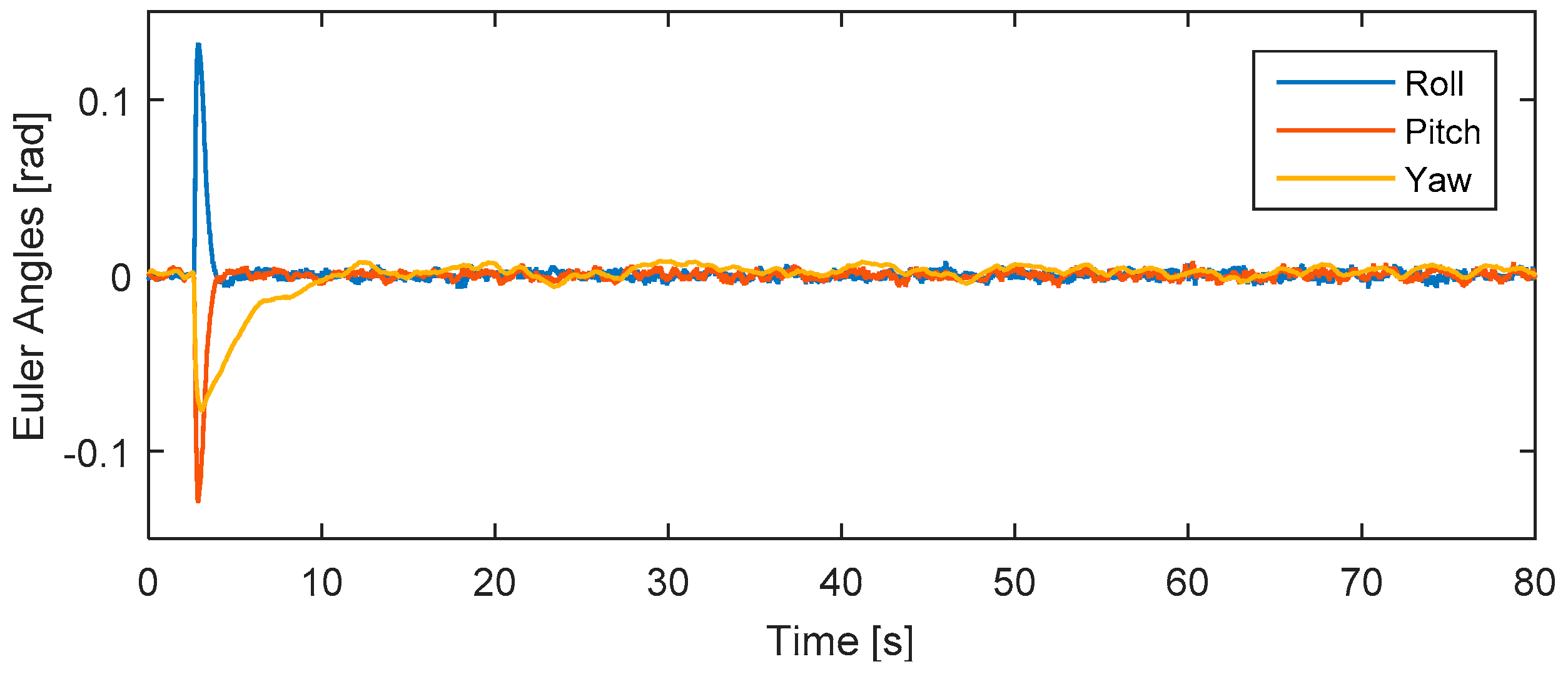
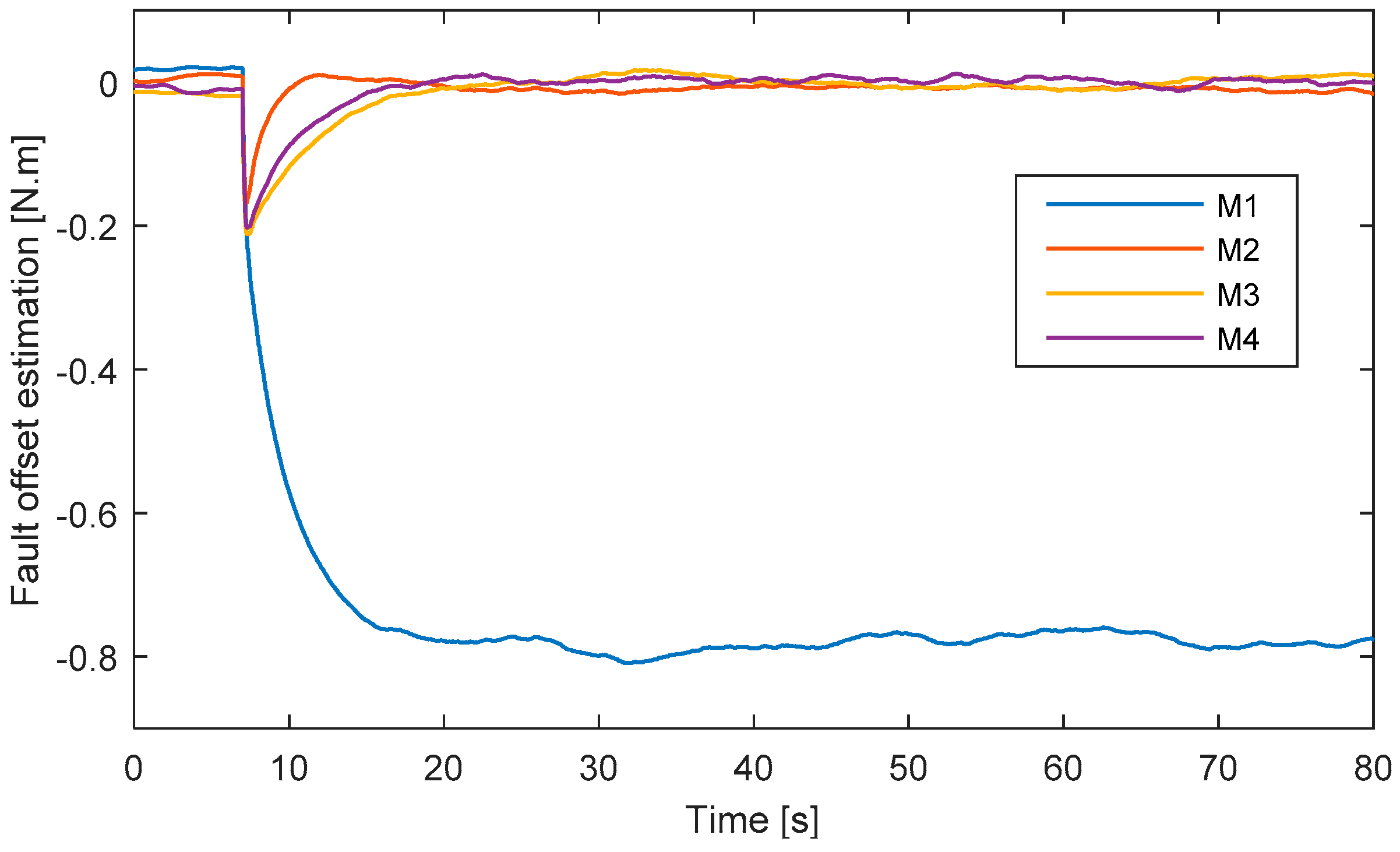
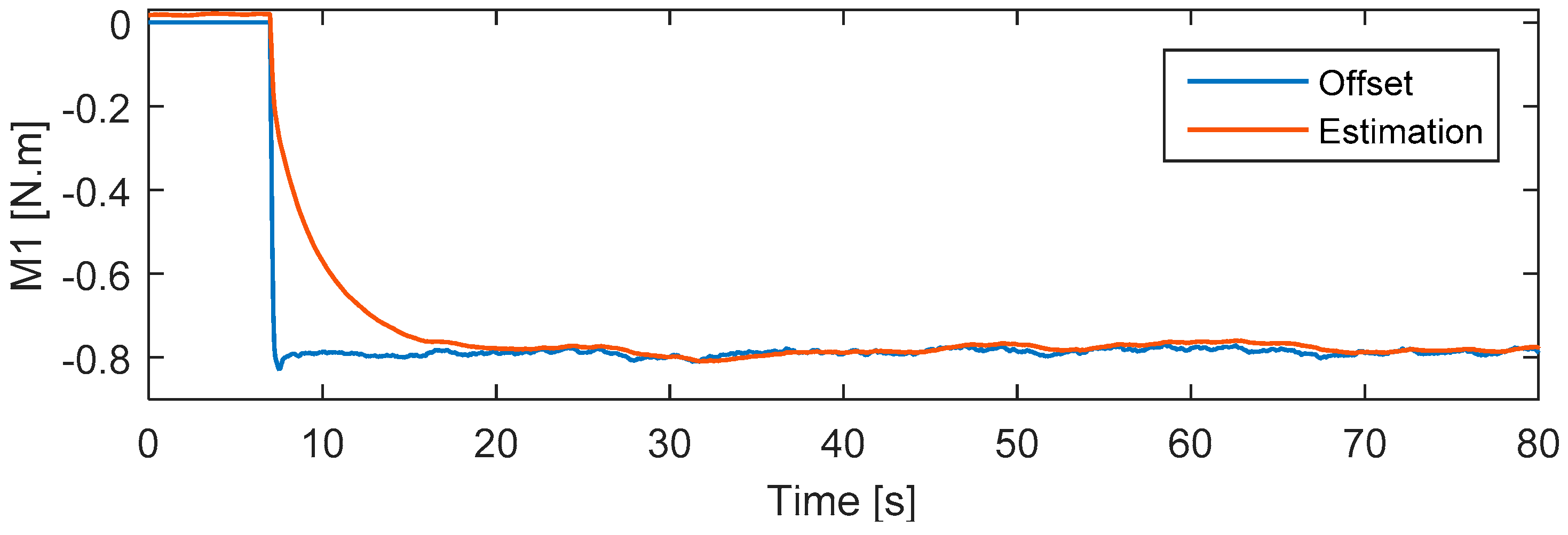
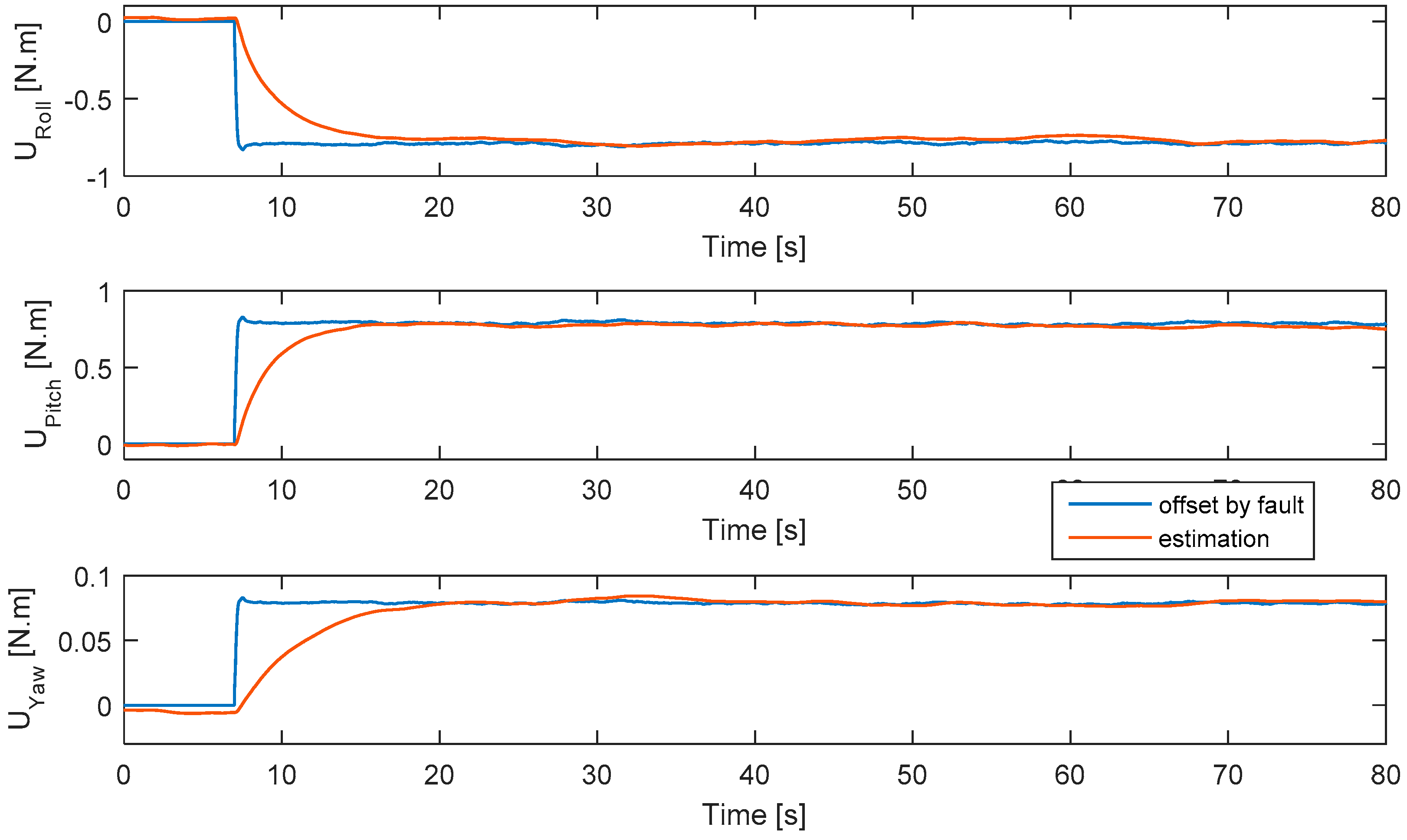
4.2. Robust Fault Diagnosis Result

The in-flight attitude response is shown in Figure 5. While Figure 6 shows the fault offset estimations M1 to M4, the real value and fault offset estimation for M1 are shown in Figure 7. It can be seen from Figure 6 that the estimation values of M2, M3, and M4 are affected by that of M1 from 7 to 18 s and, then, they converge to zero. Moreover, from the Figure 7, we see that the fault offset estimation value using ASMTO converges to the desired value with high accuracy. Figure 8 compares the real controller output offset and its estimation. From this Figure, we see that the estimation value can smoothly track the real one. Although ASMTO does not use noise filtering and identification technique for drag terms, which is presented in [20], the estimation values still obtain the high accuracy and smooth tracking.
Remark 3.
From Equations (15) and (20), it is easy to show that
e ˙ f = Γ F 2 e y + σ Γ e f + σ Γ f ( t ) f ˙ ( t ) .
The speed with which the estimation converges depends on the fault characteristics and the ASMTO design parameters. From Equation (30), we can see that Γ and σ need to be tuned in order to obtain better estimations that are adapted to the fault characteristics. Normally, the value of σ would be fixed in this algorithm.
Remark 4.
Since the moments of roll and pitch are at least one order of magnitude larger than the moment of yaw, the latter has a larger error in its fault estimation. We resolved this problem by using an amplification and reduction technique [22].
Remark 5.
The fault-tolerant controller was not the main focus of this paper, and we only used an attitude controller for the actuator fault diagnosis. Cases with more than one actuator fault were considered to be beyond the scope of this work, and were excluded mainly due to safety concerns. Moreover, the partial loss fault should be smaller than the nominal thrust of the quadcopter.

5. Conclusions

In this paper, a robust fault diagnosis method based on a Thau observer has been investigated for use on a quadcopter UAV under actuator fault, using a nonlinear modelling approach. Contrary to previous studies, the proposed scheme not only detects time-varying faults, but also works with an unknown upper bound of the associated disturbances. The stability of the error system could be demonstrated under the presence of an actuator fault. The experimental results could prove the effectiveness of this new method. In our future work, we will attempt to relax Equations (17)–(19) and implement an FTC for an attitude and position controller that will be based on the actuator fault estimation information.

Author Contributions

Conceptualization, N.P.N. and S.K.H.; Methodology, N.P.N. and S.K.H.; Software, N.P.N.; Validation, N.P.N.; Formal Analysis, N.P.N.; Investigation, N.P.N.; Resources, N.P.N.; Data Curation, N.P.N.; Writing-Original Draft Preparation, N.P.N.; Writing-Review & Editing, S.K.H.; Visualization, N.P.N.; Supervision, S.K.H.; Project Administration, S.K.H.; Funding Acquisition, S.K.H.

Funding

This research was funded and conducted under the Competency Development Program for Industry Specialists of the Korean Ministry of Trade, Industry and Energy (MOTIE), operated by Korea Institute for Advancement of Technology (KIAT), grant number N0002431.

Acknowledgments

This research was supported by Guidance, Navigation, and Control Lab at Sejong University.

Conflicts of Interest

The authors declare no conflict of interest.

References

  1. Ren, W.; Beard, R.W. Trajectory tracking for unmanned air vehicles with velocity and heading rate constraints. IEEE Trans. Control Syst. Technol. 2004, 12, 706–716. [Google Scholar] [CrossRef]
  2. Bonna, R.; Camino, J.F. Trajectory Tracking Control of a Quadcopter Using Feedback Linearization. In Proceedings of the XVII International Symposium on Dynamic Problems of Mechanics, Natal-Rio Grande Do Norte, Brazil, 22–27 February 2015. [Google Scholar]
  3. Amoozgar, M.H.; Chamseddine, A.; Zhang, Y. Experimental test of a two-stage Kalman filter for actuator fault detection and diagnosis of an unmanned quadcopter helicopter. J. Intell. Robot. Syst. 2013, 70, 107–117. [Google Scholar] [CrossRef]
  4. Chen, F.; Lei, W.; Tao, G.; Jiang, B. Actuator Fault Estimation and Reconfiguration Control for Quad-rotor Helicopter. Int. J. Adv. Robot. Syst. 2016, 13. [Google Scholar] [CrossRef]
  5. Zhao, W.; Go, T.H. Quadcopter formation flight control combining MPC and robust feedback linearization. J. Frankl. Inst. 2014, 351, 1335–1355. [Google Scholar] [CrossRef]
  6. Mahmood, A.; Kim, Y. Decentralized formation flight control of quadcopters using robust feedback linearization. J. Frankl. Inst. 2017, 354, 852–871. [Google Scholar] [CrossRef]
  7. Zhao, Q.; Jiang, J. Reliable state feedback control system design against actuator failures. Automatica 1998, 34, 1267–1272. [Google Scholar] [CrossRef]
  8. Tao, G.; Chen, S.; Joshi, S.M. An adaptive actuator failure compensation controller using output feedback. IEEE Trans. Autom. Control 2002, 47, 506–511. [Google Scholar] [CrossRef]
  9. Zhang, Y.; Jiang, J. Bibliographical review on reconfigurable fault-tolerant control systems. Annu. Rev. Control 2008, 32, 229–252. [Google Scholar] [CrossRef]
  10. Freddi, A.; Longhi, S.; Monteriù, A. A diagnostic thau observer for a class of unmanned vehicles. J. Intell. Robot. Syst. 2012, 67, 61–73. [Google Scholar] [CrossRef]
  11. Freddi, A.; Longhi, S.; Monteriù, A. A model-based fault diagnosis system for a mini-quadrotor. In Proceedings of the 2009 7th Workshop on Advanced Control and Diagnosis, Zielona Gora, Poland, 19–20 November 2009; pp. 19–20. [Google Scholar]
  12. Ma, L. Development of Fault Detection and Diagnosis Techniques with Applications to Fixed-Wing and Rotarywing UAVs. Master’s Thesis, Concordia University, Montréal, QC, Canada, 2011. [Google Scholar]
  13. Ma, L.; Zhang, Y.M. Fault detection and diagnosis for GTM UAV with dual unscented Kalman filter. In Proceedings of the AIAA Guidance, Navigation, and Control Conference, Toronto, ON, Canada, 2–5 August 2010; p. 7884. [Google Scholar]
  14. Veluvolu, K.C.; Defoort, M.; Soh, Y.C. High-gain observer with sliding mode for nonlinear state estimation and fault reconstruction. J. Frankl. Inst. 2014, 351, 1995–2014. [Google Scholar] [CrossRef]
  15. Chen, F.; Zhang, K.; Jiang, B.; Wen, C. Adaptive sliding mode observer-based robust fault reconstruction for a helicopter with actuator fault. Asian J. Control 2016, 18, 1558–1565. [Google Scholar] [CrossRef]
  16. Fekih, A.; Xu, H.; Chowdhury, F.N. Neural networks based system identification techniques for model based fault detection of nonlinear systems. Int. J. Innov. Comput. Inf. Control 2007, 3, 1073–1085. [Google Scholar]
  17. Rajakarunakaran, S.; Venkumar, P.; Devaraj, D.; Surya Prakasa Rao, K. Artificial neural network approach for fault detection in rotary system. J. Appl. Soft Comput. 2008, 8, 740–748. [Google Scholar] [CrossRef]
  18. Zhang, K.; Jiang, B.; Shi, P. Adaptive Observer-Based Fault Diagnosis with application to satellite attitude control system. In Proceedings of the Second International Conference on Innovative Computing, Information and Control, Kumamoto, Japan, 5–7 September 2007; p. 508. [Google Scholar]
  19. Wang, H.; Daley, S. Actuator fault diagnosis: An adaptive observer-based technique. IEEE Trans. Autom. Control 1996, 41, 1073–1078. [Google Scholar] [CrossRef]
  20. Li, L.; Chadli, M.; Ding, S.X.; Qiu, J.; Yang, Y. Diagnostic Observer Design for T-S Fuzzy Systems: Application to Real-Time Weighted Fault Detection Approach. IEEE Trans. Fuzzy Syst. 2018, 26, 805–816. [Google Scholar] [CrossRef]
  21. Youssef, T.; Chadli, M.; Karimi, H.R.; Wang, R. Actuator and sensor faults estimation based on proportional integral observer for TS fuzzy model. J. Frankl. Inst. 2017, 354, 2524–2542. [Google Scholar] [CrossRef]
  22. Cen, Z.; Noura, H.; Susilo, T.B.; Youmes, Y.A. Robust Fault Diagnosis for Quadrotor UAVs Using Adaptive Thau Observer. J. Intell. Robot. Syst. 2014, 73, 573–588. [Google Scholar] [CrossRef]
  23. Walcott, B.L.; Corless, M.J.; Zak, S.H. Comparative study of nonlinear state-observation techniques. Int. J. Control 1987, 45, 2109–2132. [Google Scholar] [CrossRef]
  24. Zhang, Y.; Chamseddine, A. Fault tolerant flight control techniques with application to a quadrotor UAV testbed. In Automatic Flight Control Systems—Latest Developments; Lombaerts, T., Ed.; InTech: Vienna, Austria, 2012; pp. 119–150. [Google Scholar]
  25. Zhang, K.; Jiang, B.; Cocquempot, V. Adaptive observer-based fast fault estimation. Int. J. Control Autom. Syst. 2008, 6, 320–326. [Google Scholar]
  26. Editing/Building with Eclipse on Windows. Available online: http://ardupilot.org/dev/docs/editing-the-code-with-eclipse.html (accessed on 31 August 2018).
  27. Telemetry. Available online: http://ardupilot.org/copter/docs/common-telemetry-landingpage.html (accessed on 31 August 2018).
Figure 1. Schematic of the geometric configuration of the quadcopter unmanned aerial vehicle (UAV).
Applsci 08 01893 g001
Figure 2. DJI F450 quadcopter.
Applsci 08 01893 g002
Figure 3. Experimental procedure.
Applsci 08 01893 g003
Figure 4. Motor offsets caused by the fault.
Applsci 08 01893 g004
Figure 5. The attitude angles.
Applsci 08 01893 g005
Figure 6. Fault estimation.
Applsci 08 01893 g006
Figure 7. M1 offset by fault and its estimation.
Applsci 08 01893 g007
Figure 8. Controller output offset by fault and its estimation.
Applsci 08 01893 g008
Table 1. DJI F450 quadcopter parameters.
ParameterDescriptionValue
L Arm length 0.225 m
b Thrust coefficient 9.8 × 10 6 N/m2
d Drag coefficient 1.6 × 10 7
mMass 2 kg
I x ;   I y ;   I z Moments of inertia 0.0035 ;   0.0035 ;   0.005 kg·m2
J T Rotor inertia 2.8 × 10 6 kg·m2

