Live Convolution with Time-Varying Filters

Abstract

The paper presents two new approaches to artefact-free real-time updates of the impulse response in convolution. Both approaches are based on incremental updates of the filter. This can be useful for several applications within digital audio processing: parametrisation of convolution reverbs, dynamic filters, and live convolution. The development of these techniques has been done within the framework of a research project on crossadaptive audio processing methods for live performance. Our main motivation has thus been live convolution, where the signals from two music performers are convolved with each other, allowing the musicians to “play through each other’s sound”.

1. Introduction

Convolution has been used for filtering, reverberation, spatialisation, and as a creative tool for cross-synthesis in a variety of contexts [1,2,3,4,5]. Common to most of them is that one of the inputs is a time-invariant impulse response (characterising a filter, an acoustic space or similar), allocated, and preprocessed prior to the convolution operation. Although developments have been made to make the process latency free (using a combination of partitioned and direct convolution [6]), the time-invariant nature of the impulse response (IR) has inhibited a parametric modulation of the process. Modifying the IR traditionally has implied the need to stop the audio processing, load the new IR, and then re-start processing using the updated IR. The methods presented in this paper represents two new approaches to allow real-time modifications of the IR without interrupting the audio processing. The IR updates can be done without introducing artefacts in the audio output. Research on these methods were initiated within the project “Cross-adaptive processing as musical intervention” [7] investigating various kinds of signal interaction between audio signals from two or more live music performers. Convolution as a method for signal interaction was found desirable in the context of this research, but methods of facilitating the convolution of two live signals were needed to enable the performers to flexibly interact with the process. One of the methods presented here have been discussed by two of the authors in an earlier conference paper [8], where artefact-free updates of the filter allowed live sampling of the impulse response. The current paper expands on this work by adding another method for time-varying filter coefficients. Both methods for filter updates are based on a similar concept, where coefficients are replaced at audio rate, enabling artefact free transition from old to new filter coefficients, even with arbitrary different coefficients. Software tools from the conference paper have also been expanded to include both filter methods. A number of practical experiments in studio and live sessions have been done during the time since the conference paper was written. Reflections on these artistic explorations have been included in the present article.

1.1. Time-Varying Filters

Time-varying convolution has been explored in continuous-time systems [9], and in discrete-time systems, both finite impulse response (FIR) and infinite impulse response (IIR) coefficient-modulated filters have been extensively discussed in [10]. Applications are numerous and include, for instance, speech processing [11,12], equalization of audio signals [13,14,15], binaural processing [16,17], and reverberation [6,18].

Digital time-varying filters in music are typically composed of recursive filter structures of lower order and proposed approaches are particularly concerned with stabilization and transient suppression [13,19]. Strategies reported include intermediate sets of filter coefficients [15,20,21], state variable updates [11,19], and input-switching [12].

The present paper is concerned with impulse responses live sampled from audio signals. The filter order is also substantially higher than in the approaches listed above, since the audio samples involved may possibly last several seconds. Hence, we are specifically looking at time-varying FIR filters that can be dynamically updated without perceptual artefacts. Virtual acoustic reality is another application area where convolution with time-varying FIR filters find use [16,17,22]. One possible approach to avoid perceptual artefacts is to cross-fade between the outputs of several simultaneous convolution processes [23]. However, this gets prohibitively expensive for audio-rate filter updates. Jot, Larchel, and Warusfel [17] suggests incremental filter switching at high update rates (referred to as commutation) for binaural processing, while Lee et al. [18] suggests a similar approach for artificial late-field reverberation where the rate of change may adapt to characteristics of the input. These strategies minimize the artefacts, but at the cost of computing intermediate filters. Vickers [24] presents a number of frequency-domain strategies for time-varying FIR filters. In general, the solutions either violate the constraints of linear convolution and produce artefacts, or they demand extra processing power: typically more than twice the number of real multiplications per output sample compared to the common convolution implementation overlap-add short-time Fourier Transform (OLA STFT).

Instead, we will present two different techniques that perform dynamic, low-latency convolution of live-sampled impulse responses with negligible computational overhead.

1.2. Convolution and Other Sound Transformations, Live Use

Techniques for signal interaction in creative sound design have been widely used. Among these, we find Ring modulation (an early example of artistic use is Stockhausen’s “Mixtur” from 1964, and an example from popular music is Black Sabbath’s “Paranoid” from 1970), Vocoder (popularized by Wendy Carlos in the music for Stanley Kubrick’s “A Clockwork Orange” from 1971, another popular example is Laurie Anderson’s “O Superman” from 1981), Talk box (an early use by Joe Walsh in “Rocky Mountain Way”, and popularized by Peter Frampton in various contexts), and Auto-Wah (popularized by Stevie Wonder on songs like “Superstition” and “Higher Ground” from the early 1970s). Contemporary electronic dance music also make extensive use of signal interaction by means of sidechain compression to create “pumping” effects (a classic example is Eric Prydz’ “Call On Me” from 2004). Common to all of these methods is the immediate use of a feature from one sound to control some modulation of another (or the same) sound. The same can be said about other feature-based modulation methods used in our crossadaptive research project. Convolution has the added feature that preserves the full spectrotemporal structure of the modulation sound. Not only is it using the spectrum of one sound to filter another sound, but the temporal evolution of the modulating sound’s spectrum is preserved in the filtering. Realtime spectral transformations and cross synthesis (Dynamic filtering of one signal, using the spectral envelope of another signal) has been explored during the last 30 years or so together with convolution [1,25]. Creative uses of convolution as a timbral transformative device in composition has been explored by [3,4,5,26,27], and the more performative aspects of real-time convolution by [28,29,30]. Common to all of these has been that the impulse response of the convolution process was static, and that any updates or dynamic replacement of the impulse response required some variation of a crossfading scheme between parallel convolution processes. With our currently described methods, we can update the impulse response with audio content captured from a live performance. This can be seen as a form of live sampling:

“Live sampling during performance.... uses the Now as its subject” [31].

Live sampling has been used as a method for creating temporal dynamism and a heightened sense of the Now. Perhaps the earliest occurence is in Mauricio Kagel’s composition “Transición II” from 1958 [32], and the idea was further developed during the following decades amongst others by Kaffe Mathews and by Michael Waisvisz [33]. Live looping by means of improvisation instruments with long delay lines has been explored by Lawrence Casserley [34] in the Evan Parker Electroacoustic Ensemble, while utilisation in pop music have been done by artists Ed Sheeran, Boxwood, and others. In our current research project, we wanted to investigate the potential of live sampling the impulse response, to enable an even more intimate interaction between live sources than previously had been possible within real-time convolution and live sampling as separate domains. The recontextualisation of an audio sample recorded during the same performance, used as the acoustic environment in which the other musician can perform.

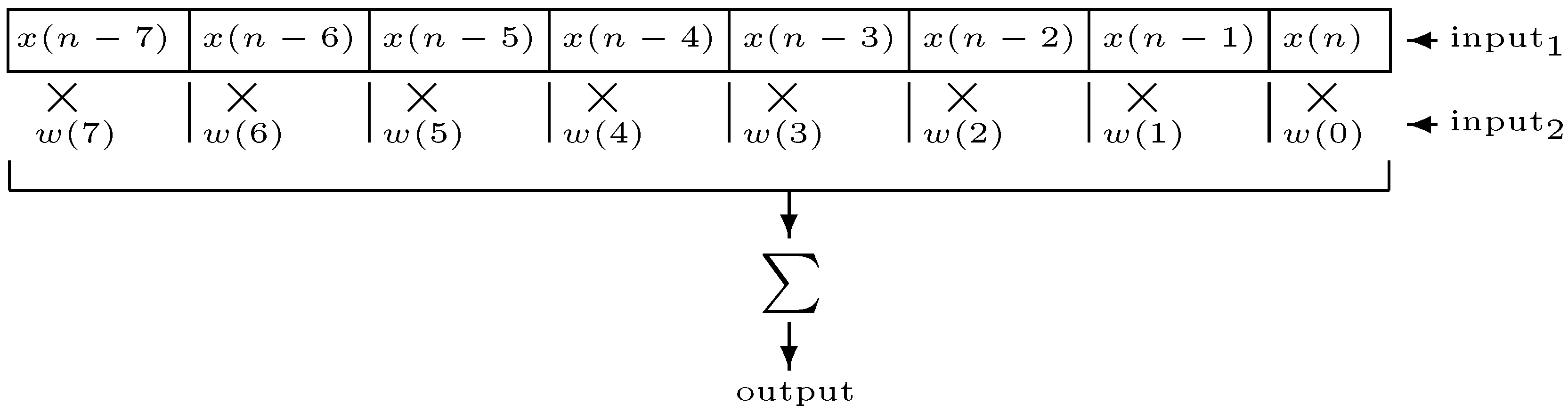
2. Time-Varying Finite Impulse Response Filters

A digital finite impulse response filter (FIR) of length N is defined by the following difference equation [35]:

$$\begin{array}{cc}\hfill y\left(n\right)& =a_{0}x\left(n\right)+a_{1}x(n-1)+\dots +a_{N-1}x(n-[N-1])\hfill \\ & ={\displaystyle \sum _{k=0}^{N-1}}{a}_{k}x(n-k),\hfill \end{array}$$

(1)

where $x\left(n\right)$ and $y\left(n\right)$ are the input and output signals, respectively, at time n, and $a_0$ to $a_{N-1}$ are the scaling coefficients of each copy of the input signal delayed by 0 to $N-1$ samples (in this text, we will use the convention that a filter with length N has order $N-1$). When these coefficients are unchanging, the filter is a linear time-invariant filter.

For an FIR filter, its set of coefficients also make up the filter impulse response $h\left(n\right)$, which is the output of the filter when fed with a unit sample signal $u\left(n\right)$, which is 1 for $n=0$ and 0 elsewhere:

$$h\left(n\right)={\displaystyle \sum _{k=0}^{N-1}}{a}_{k}u(n-k)=a_n.$$

(2)

The output signal $y\left(n\right)$ can then be expressed as the convolution of input signal $x\left(n\right)$ and impulse response $h\left(n\right)$ (convolution is a commutative operation):

$$y\left(n\right)={\displaystyle \sum _{k=0}^{N-1}}h(n-k)x\left(k\right)={\displaystyle \sum _{k=0}^{N-1}}h\left(k\right)x(n-k).$$

(3)

The spectrum of the filter impulse response defines its frequency response, which determines how the filter modifies the input signal amplitudes and phases at different frequencies. A generalised form of this, called the filter transfer function can be obtained via the z-transform,

$$H\left(z\right)={\displaystyle \sum _{n=-\infty }^{\infty }}h\left(n\right)z^{-n},$$

(4)

which is a function of the complex variable z. In the usual case that the filter is of finite length N, we have:

$$H\left(z\right)={\displaystyle \sum _{n=0}^{N-1}}h\left(n\right)z^{-n}={\displaystyle \sum _{n=0}^{N-1}}{a}_n{z}^{-n}.$$

(5)

By setting $z=e^{j\omega }$ and $\omega =2\pi k/N$, we can compute the filter spectrum via the discrete Fourier transform (DFT). This is called the filter frequency response. The effect of a filter in the spectral domain is defined by the following expression:

$$Y\left(z\right)=H\left(z\right)X\left(z\right),$$

(6)

and thus it is possible to implement the filter either in time domain as a convolution operation (Equation (3)) or in the frequency domain as a product of two spectra.

We would like to examine the cases where these coefficients in Equation (1) are not fixed, which characterizes the filter as time-varying (TV). The most general expression for a TVFIR is defined as follows [10]:

$$\begin{array}{cc}\hfill y\left(n\right)& =a_0\left(n\right)x\left(n\right)+a_1\left(n\right)x(n-1)+\dots +a_{N-1}\left(n\right)x(n-[N-1])\hfill \\ & ={\displaystyle \sum _{k=0}^{N-1}}{a}_k\left(n\right)x(n-k),\hfill \end{array}$$

(7)

where we assume that the filter coefficients are drawn each from a digital signal $a_k\left(n\right)$. In this case, the impulse response will vary over time and thus becomes a function of two time variables, m and n, representing time of input signal application and time of observation, respectively:

$$h(m,n)={\displaystyle \sum _{k=0}^{N-1}}{a}_k\left(n\right)u(n-m-k).$$

(8)

The output of this filter is defined by the expression

$$y\left(n\right)={\displaystyle \sum _{m=-\infty }^{\infty }}h(m,n)x\left(m\right).$$

(9)

Since the output can only appear after the input is applied ($x\left(n\right)=0$ for $n<0$), the impulse response $h(m,n)=0$ for $n<0$ and $n<m$. If we then substitute $l=n-m$, we get the convolution

$$y\left(n\right)={\displaystyle \sum _{l=0}^n}h(n-l,n)x(n-l).$$

(10)

The transfer function also becomes a function of two variables, z and n, and assuming causality we get:

$$H(z,n)={\displaystyle \sum _{m=0}^n}h(m,n)z^{m-n}={\displaystyle \sum _{k=0}^{N-1}}{a}_k\left(n\right)z^{-k}.$$

(11)

The next two sections present two different approaches to time-varying filtering: Dynamic replacement of impulse responses and convolution with continuously varying filters.

3. Dynamic Replacement of Impulse Responses

We first examine filter impulse responses where the coefficients are not continuously changing, but are replaced at given points in time. This approach was first presented in [8], but is given a more detailed explanation here. It is related to the superposition strategy suggested by Verhelst and Nilens [12]: when a filter change is called for, the signal input is disconnected from the currently running filter and applied to the new one. The old filter is left free-running, i.e., the old input samples propagate through the filter, and will eventually die out (for FIR filters after a time period equivalent to the filter length). The outputs of the two filters are added together. The next change adds another filter, and so on. To make this work, a number of filter processes must run in parallel.

Our approach differs from Verhelst and Nilens in that we propose to run all filters in the same filter process, simply by switching the new filter, coefficient by coefficient, into the same filter buffer as the old one. We claim that, for FIR filters, the results produced by the two approaches are equal, but that our approach avoids the added computational cost of computing two or more parallel convolution processes. By exploiting inherent properties of convolution, we also show that we may start convolving with the new filter impulse response in parallel with the generation/recording of it.

As an initial step consider a simple filter of length N that is switched on at a given time index $n_s$:

$$h_E(m,n)=\left\{\begin{array}{cc}0,\hfill & m<n_s,\hfill \\ e_{n-m},\hfill & m\ge n_s,\hfill \end{array}\right.$$

(12)

It should be obvious that inputs $x\left(n\right)$ for $n<n_s$ will not contribute to the output. If we apply Equation (10) and once again let $l=n-m$, the first N samples of convolution output starting at time index $n_s$ can be written as:

$$y\left(n\right)={\displaystyle \sum _{l=0}^{n-n_s}}{e}_{l}x(n-l)(n_s\le n\le n_s+N-1).$$

(13)

After $n=n_s+N-1$ the sum will be upper limited by $l=N-1$. The first output sample, $y\left(n_s\right)$, depends on the first coefficient, $e_0$ only. The second sample, $y(n_s+1)$, depends on the first two, $e_0$ and $e_1$. In general, $y(n_s+k)$ depends on coefficient $e_l$ only if $l\le k$. Hence, the filter coefficients can be switched in one by one in parallel with the running convolution process.

Now consider the counterpart, a filter of length N that is switched off at the same time index $n_s$ (and for simplicity assume that $n_s>N$, the filter length):

$$h_C(m,n)=\left\{\begin{array}{cc}{c}_{n-m},\hfill & m<n_s,\hfill \\ 0,\hfill & m\ge n_s.\hfill \end{array}\right.$$

(14)

Inputs $x\left(n\right)$ for $n\ge n_s$ will not contribute to the output. The first N samples of convolution output starting at $n_s$ can be written as:

$$y\left(n\right)={\displaystyle \sum _{l=n-n_s+1}^{N-1}}{c}_{l}x(n-l)(n_s\le n\le n_s+N-1).$$

(15)

The first output sample, $y\left(n_s\right)$, does not depend on the first coefficient, $c_0$. The second sample, $y(n_s+1)$, does not depend on the first two, $c_0$ and $c_1$. In general, $y(n_s+k)$ does not depend on coefficient $c_l$ if $l\le k$.

The natural extension of these two filters is the combined filter $h_{C+E}$ where the coefficients are replaced at time index $n_s$:

$$h_{C+E}(m,n)=\left\{\begin{array}{cc}{c}_{n-m},\hfill & m<n_s,\hfill \\ e_{n-m},\hfill & m\ge n_s.\hfill \end{array}\right.$$

(16)

The first N samples of convolution output starting at $n_s$ must be equal to the sum of the two filters discussed above:

$$y\left(n\right)={\displaystyle \sum _{l=0}^{n-n_s}}{e}_{l}x(n-l)+{\displaystyle \sum _{l=n-n_s+1}^{N-1}}{c}_{l}x(n-l)(n_s\le n\le n_s+N-1).$$

(17)

A closer scrutiny reveals that coefficients $e_l$ and $c_l$ do not contribute to the same output sample $y\left(n\right)$ for any $l,n$. In fact, the filter coefficients $c_l$ may be replaced with $e_l$ one by one during the transition interval $[n_s,n_s+N-1]$, while the convolution is running. The replacement itself will not introduce output artefacts as long as the coefficients are replaced just in time and in the correct order.

For completeness, we will examine a third filter of length N where the coefficients are replaced at two different times, $n_{s1}$ < $n_{s2}$:

$$h_{C+D+E}(\tau ,t)=\left\{\begin{array}{cc}{c}_{m-n},\hfill & m<n_{s1},\hfill \\ d_{m-n},\hfill & n_{s1}\le m<n_{s2},\hfill \\ e_{m-n},\hfill & m\ge n_{s2}.\hfill \end{array}\right.$$

(18)

If the time interval $n_{s2}-n_{s1}>N$, then the two transition regions $[n_{s1},n_{s1}+N-1]$ and $[n_{s2},n_{s2}+N-1]$ each behave as in Equation (17). If not, we get a subinterval $[n_{s2},n_{s1}+N-1]$ of the transition region where all three filters contribute to the output:

$$y\left(n\right)={\displaystyle \sum _{l=0}^{n-n_{s2}}}{e}_{l}x(n-l)+{\displaystyle \sum _{l=n-n_{s2}+1}^{n-n_{s1}}}{d}_{l}x(n-l)+{\displaystyle \sum _{l=n-n_{s1}+1}^{N-1}}{c}_{l}x(n-l)(n_{s2}\le n\le n_{s1}+N-1).$$

(19)

Similar to the above, the coefficients $e_l$, $d_l$, and $c_l$ do not contribute to the same output sample $y\left(n\right)$ for any $l,n$. Hence, several filter replacements may be carried out simultaneously without artefacts. However, the number of coefficients involved in the convolution sum will be limited by the interval $[n-n_{s2}+1,n-n_{s1}]$ as seen in the middle term above, for a total of $(n_{s2}-n_{s1})$ summands. An alternative view of this filter replacement scheme is that the input signal $x\left(n\right)$ is split in segments $[0,n_{s1}-1]$, $[n_{s1},n_{s2}-1]$, and $[n_{s2},\infty )$ each convolved with just one set of coefficients, $c_l$, $d_l$, and $e_l$, respectively. The output is the sum of contributions from all three filters.

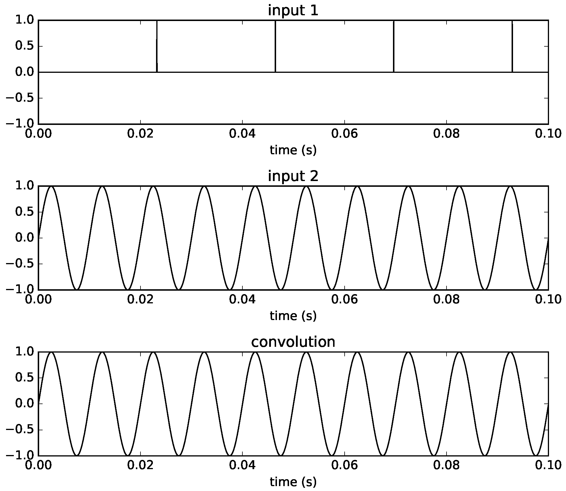
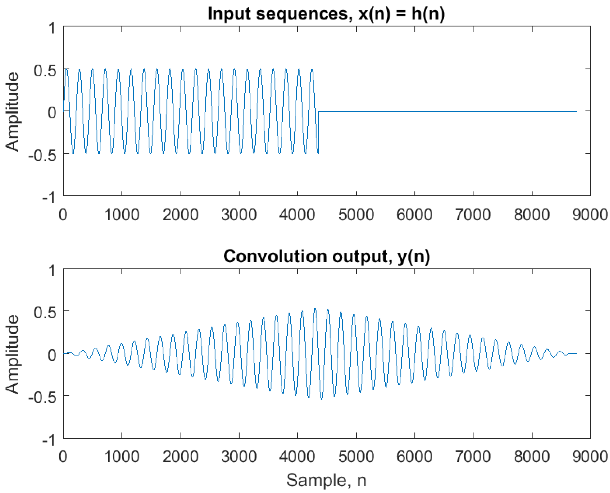
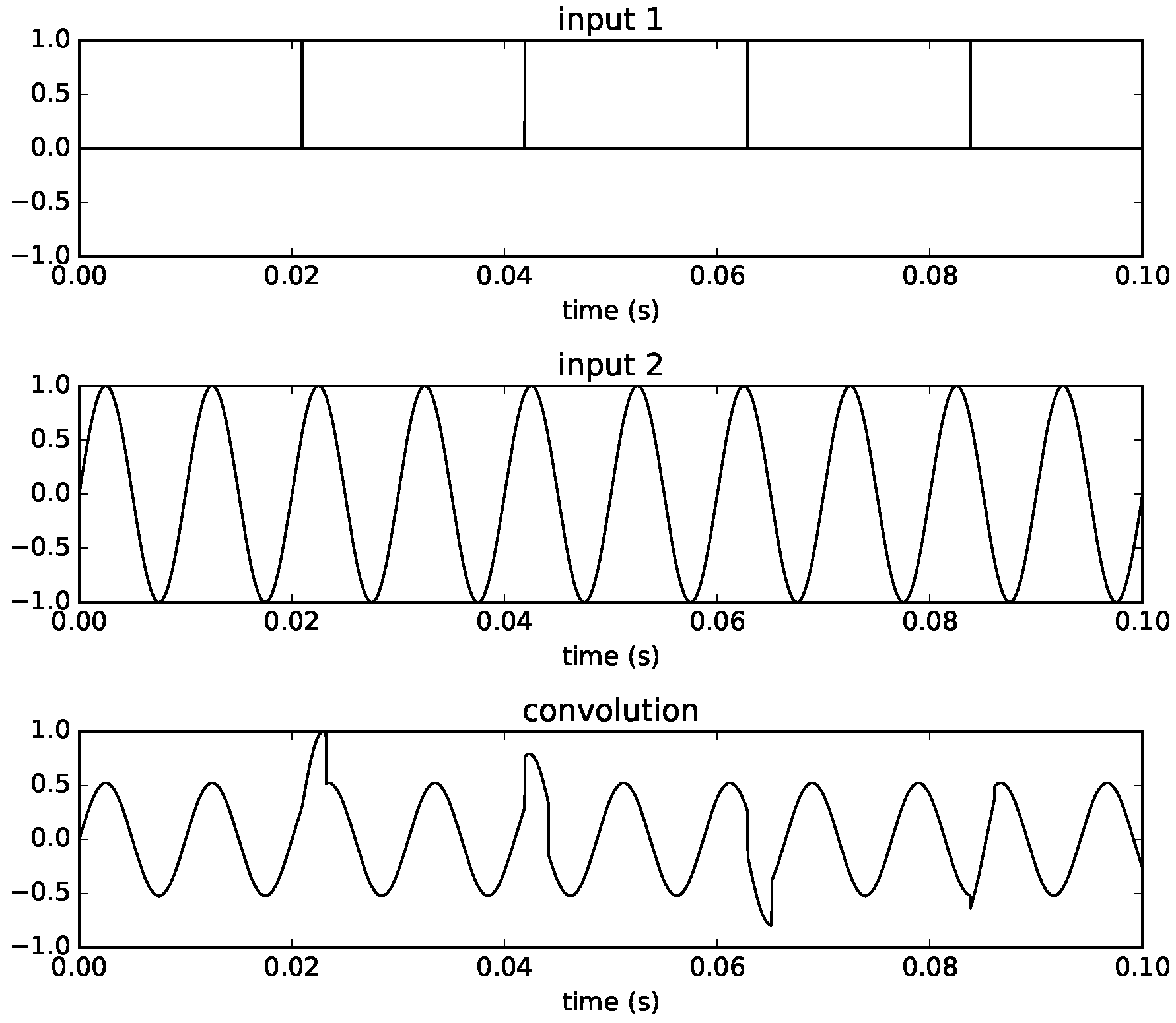
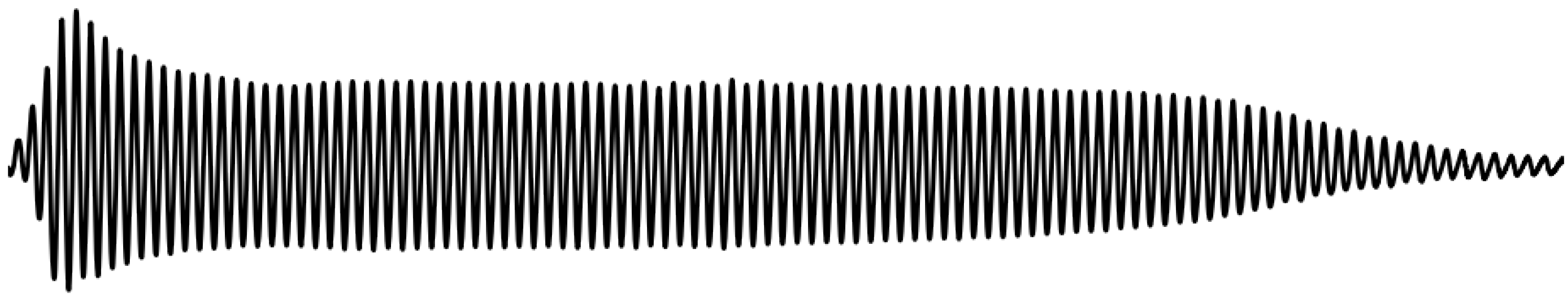
Convolution has by nature a ramp characteristic as exemplified in Figure 1 where a simple sinusoidal signal time-limited by a rectangular window is convolved with itself ($x\left(n\right)=h\left(n\right)$). When doing a gradual replacement of filter coefficients, this inherent ramp characteristic ensures a smoothly overlapping transition region between the filters $h_C$ and $h_E$.

This technique of stepwise filter replacement outperforms other methods of dynamic filter updates:

• It avoids the discontinuities and artefacts caused by instantaneous switching between filters. It makes no assumptions on similarity between filters as in the commutation [17] or on input signal properties as for the switched convolution reverberator [18].
• It saves the computational effort necessary to superpose or cross-fade parallel convolution processes [12,22].
• It provides the minimum possible latency for a filter update and even allows convolution with a filter to start in parallel with the generation/recording of the filter impulse response itself.

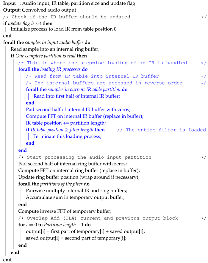
When filter length increases direct convolution in the time-domain is normally replaced with computationally more efficient methods in the frequency domain. A popular approach is partitioned convolution [6,36] where the filter impulse response and the input signal are broken into partitions and the convolution computed as multiplication of these partitions in the frequency domain (more on implementation in Section 5). The method of stepwise filter replacement still works, but now the partition is the unit of replacement. Replacement must be initiated at a time index $n_s$ equal to an integer multiple of the partition length $N_P$: $n_s=k{N}_P$. A latency equal to the partition length $N_P$ is also introduced.

Example

In order to illustrate the behavior of dynamic replacement of filter impulse responses, we present a simple example. Figure 2 shows the input signals to a convolution process. On top are the two impulse responses $h_A\left(n\right)$ and $h_B\left(n\right)$. They are both sinusoidal signals of duration 1.5 s sampled at 44,100 Hz and with a frequency of 60 and 10 Hz, respectively. At the bottom is the input signal $x\left(n\right)$, which is an impulse train with pulses at 0.3 s interval, also sampled at 44,100 Hz.

These signals are convolved using partitioned convolution (overlap-add STFT) with partition length $N_P$ = 256 and FFT block size $N_B$ = 512. At time index $n_s$ = 1 s, a switch between the two impulse response filters is performed.

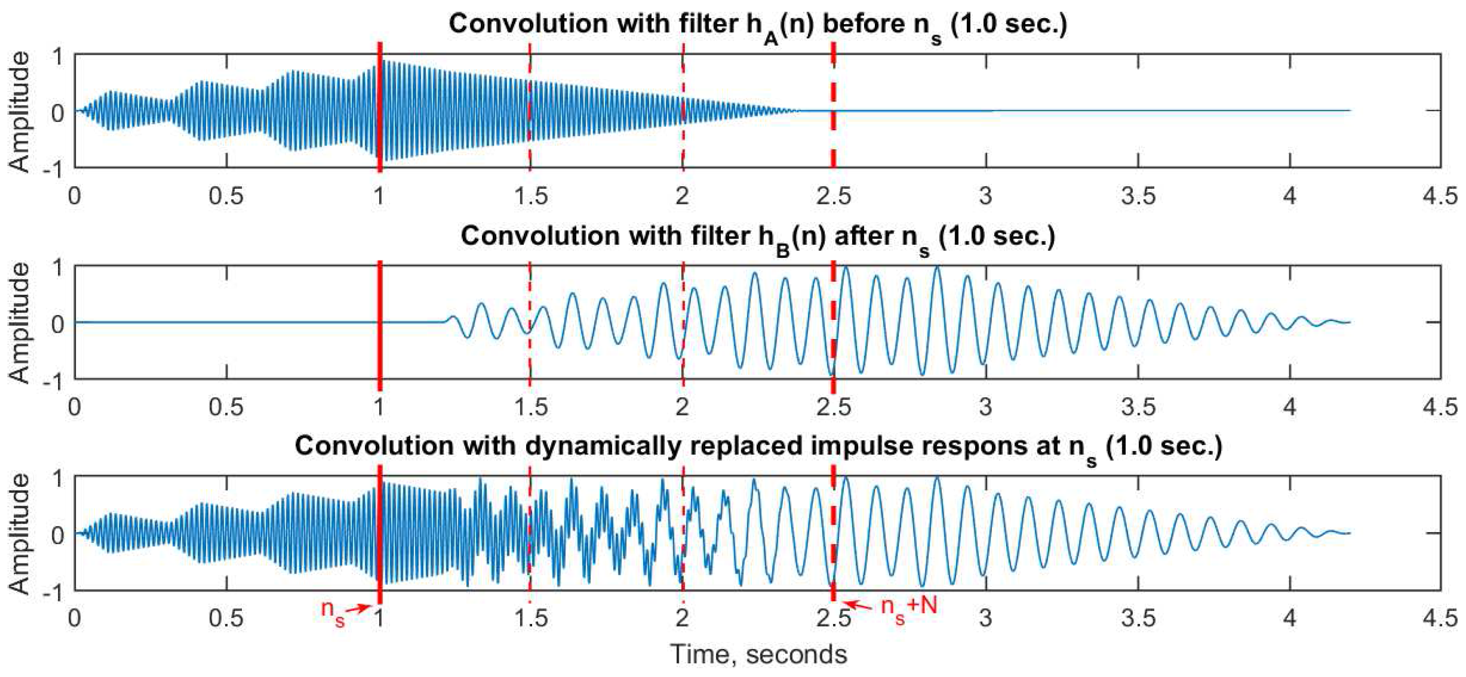
Figure 3 shows the results. At the top is the output from convolving the input signal $x\left(n\right)$ with impulse response $h_A\left(n\right)$, but only up to the time index $n_s$. Notice the convolution tail between 1.0 and 2.5 s, equal to the filter length. In the middle is the output from convolving the input signal $x\left(n\right)$ with impulse response $h_B\left(n\right)$ starting after the time index $n_s$. Finally, at the bottom, we show the output from convolving the input signal $x\left(n\right)$ with both filters, such that $h_A\left(n\right)$ is stepwise replaced by $h_B\left(n\right)$ starting at time index $n_s$, following the scheme introduced in the previous section. The important thing to note here is that an identical result is achieved if we instead add together the two partial outputs (top and middle).

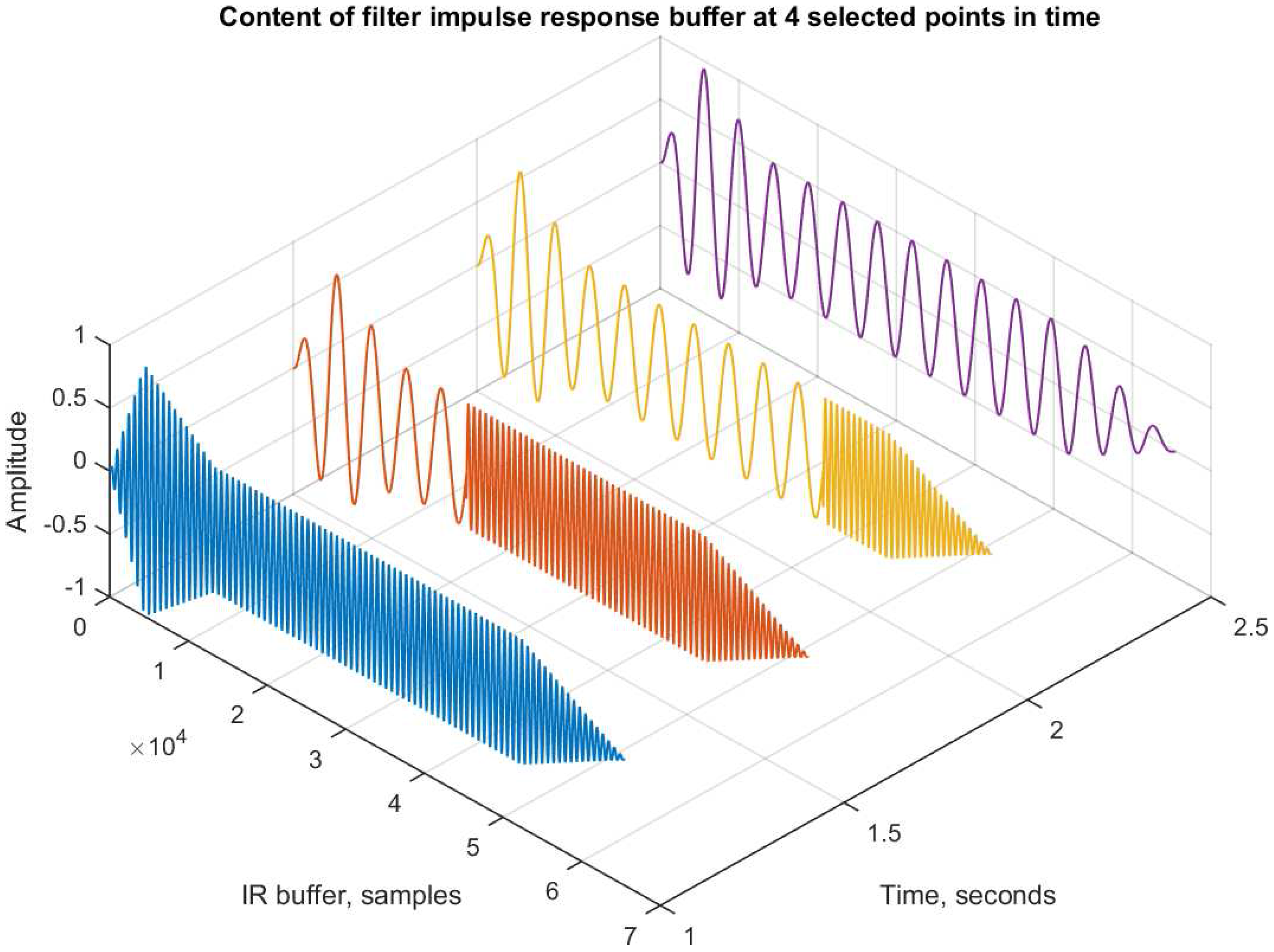
The convolution process is working on a single impulse response buffer. During the filter transition, the buffer will contain parts of both the filters $h_A\left(n\right)$ and $h_B\left(n\right)$. Figure 4 illustrates the content of the buffer at four different points in time. Just before transition ($n_s$ = 1 s), the buffer is entirely filled with impulse response $h_A\left(n\right)$. During the transition (1.5 and 2.0 s), we notice how the buffer is gradually filled with impulse response $h_B\left(n\right)$, starting from sample 0. After the transition ($n_s+N-1$ = 2.5 s), the buffer is entirely filled with impulse response $h_B\left(n\right)$.

There are noticeable discontinuities in the buffer content during transition, but it is important to realize that each of these buffer snapshots will be multiplied with the input $x\left(n\right)$ to produce a single output sample. They are not temporal objects per se. As mentioned earlier, the method is equivalent to segmenting the input signal at the time $n_s$: any input $x\left(n\right)$, $n<n_s$ convolves with filter $h_A\left(n\right)$ only. Any input $x\left(n\right)$, $n\ge n_s$ convolves with filter $h_B\left(n\right)$ only.

4. Time-Varying Convolution

Time-varying filters whose coefficients are changing at audio rates, as is the case here, have many applications in music [13,37,38]. In particular, some significant attention has been dedicated to infinite impulse response types that whose coefficients are modulated by a periodic signals [39,40,41,42]. These filters tend to be of lower order (first or second order), which have equivalent longer forms made up of two sections arranged in series, a TVFIR and a fixed-coefficient IIR [41]. It has also been shown that the most significant part of the effect of these filters is contained in the TVFIR component.

The case we will examine here presents a TVFIR whose coefficients are taken from an arbitrary input waveform, segmented by the filter length N. This is formally defined by employing the sequence $w\left(n\right)$ as the set of N filter coefficients starting at a given time index n:

$$a_k\left(n\right)=w(n+k)(0<k<N-1).$$

(20)

This expression involves future values of $w\left(n\right)$ and needs to be adapted so that we can calculate the signal $y\left(n\right)$ based solely on the current and past values of the inputs. Furthermore, if we are to calculate successive values of $a_k\left(n\right)$, the following expression should apply:

$$a_k(n+1)=a_{k+1}\left(n\right),$$

(21)

from which we should note that the complete set of N filter coefficients will differ only by one value as the current time index n increments by one. If we compare the first N samples of $w\left(n\right)$ and $w(n+1)$, we will observe that they share $N-1$ values. To get the N coefficients $a_k(n+1)$, we only need to discard $a_0\left(n\right)$, shift all samples by one position to the left, and replace the last sample of the sequence by a new value $w(n+N)$. We can do this efficiently by applying a circular shift in the coefficients based on the filter size and current time. In this scenario, a set of N coefficient functions $c_k\left(n\right)$ can be defined as

$$c_k\left(n\right)=\left\{\begin{array}{cc}w\left(n\right),\hfill & k=n\mathrm{mod}\mathrm{N},\hfill \\ c_k(n-1),\hfill & \mathrm{otherwise},\hfill \end{array}\right.$$

(22)

where each one of the coefficients will change only once every N samples, as the signal $w\left(n\right)$ is taken in by the filter. They will hold their values until a their update time is due. Using this set of coefficients $c_k\left(n\right)$ as defined in Equation (22), the TVFIR filter expression becomes (assuming that $c_k\left(n\right)=0$, $w\left(n\right)=0$, and $x\left(n\right)=0$ for $n<0$)

$$\begin{array}{cc}\hfill y\left(n\right)& =c_0\left(n\right)x\left(n\right)+c_1\left(n\right)x(n-1)+\dots +c_{N-1}\left(n\right)x(n-N-1)\hfill \\ & ={\displaystyle \sum _{k=0}^{N-1}}{c}_k\left(n\right)x(n-k),\hfill \end{array}$$

(23)

which defines what in this paper we call time-varying convolution (to distinguish it from the more general forms of TVFIR filters, even though in the other cases the convolution is actually also time varying). In this scenario, we are interpreting an arbitrary input signal of length N as an impulse response, and allow it to vary on a sample-by-sample basis. The resulting set of coefficients $c_k$, derived from $w\left(n\right)$, is completely replaced every N samples. There is, in fact, no particular distinction between the two inputs to the system ($x\left(n\right)$ and $w\left(n\right)$), and we may wish to view either as the “filtered” signal or the “impulse response”. Taking one of these, e.g., $w\left(n\right)$, as the filter coefficients, we can determine the filter frequency response for an input $x\left(n\right)$ from the filter transfer function, which has to be determined at every sample. 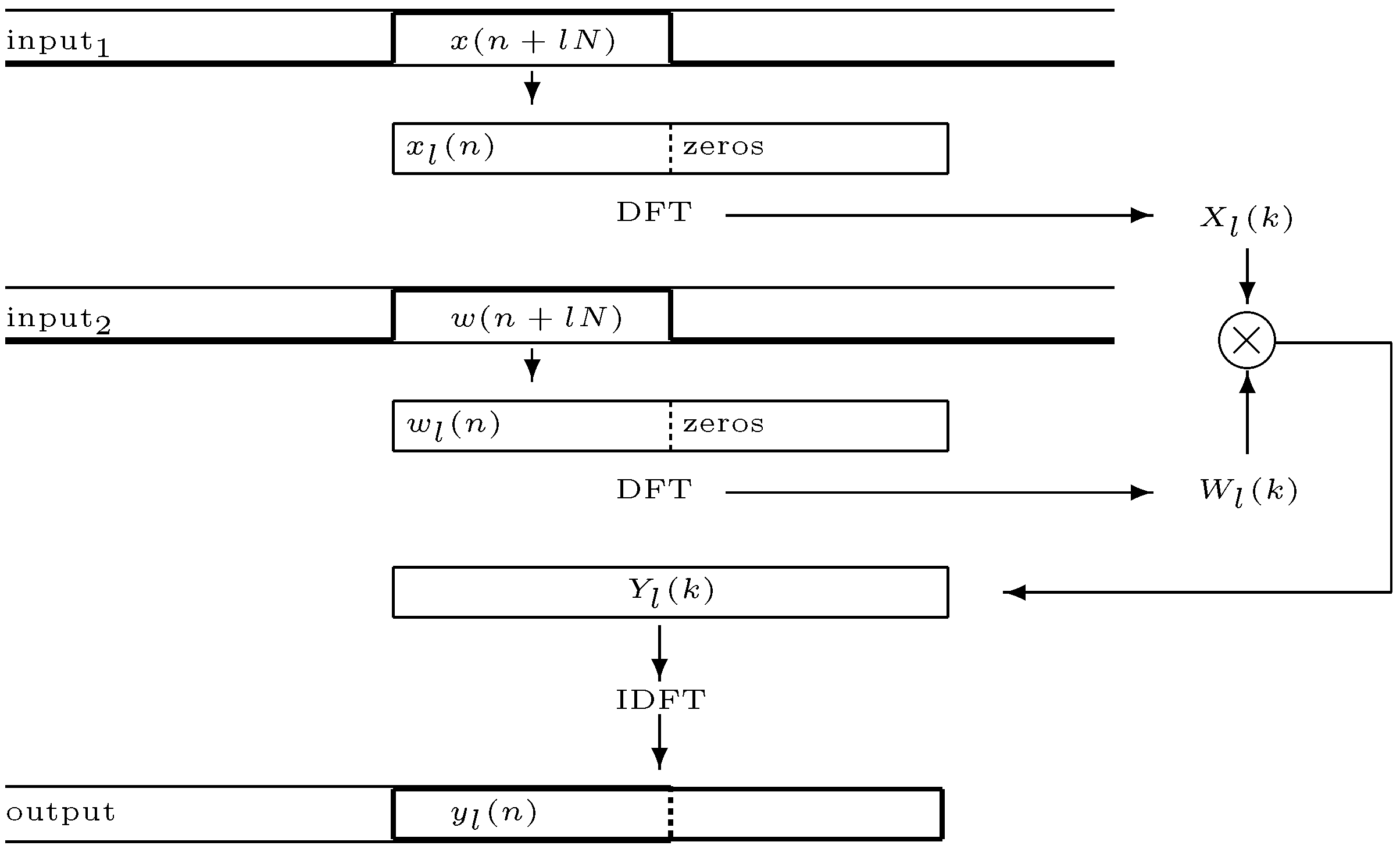This becomes then a function of two variables, frequency k and time n, and can be evaluated by taking its DFT at every N samples:

$$W(n,k)={\displaystyle \sum _{m=0}^{2N-1}}{w}_n\left(m\right)e^{-j\omega k},$$

(24)

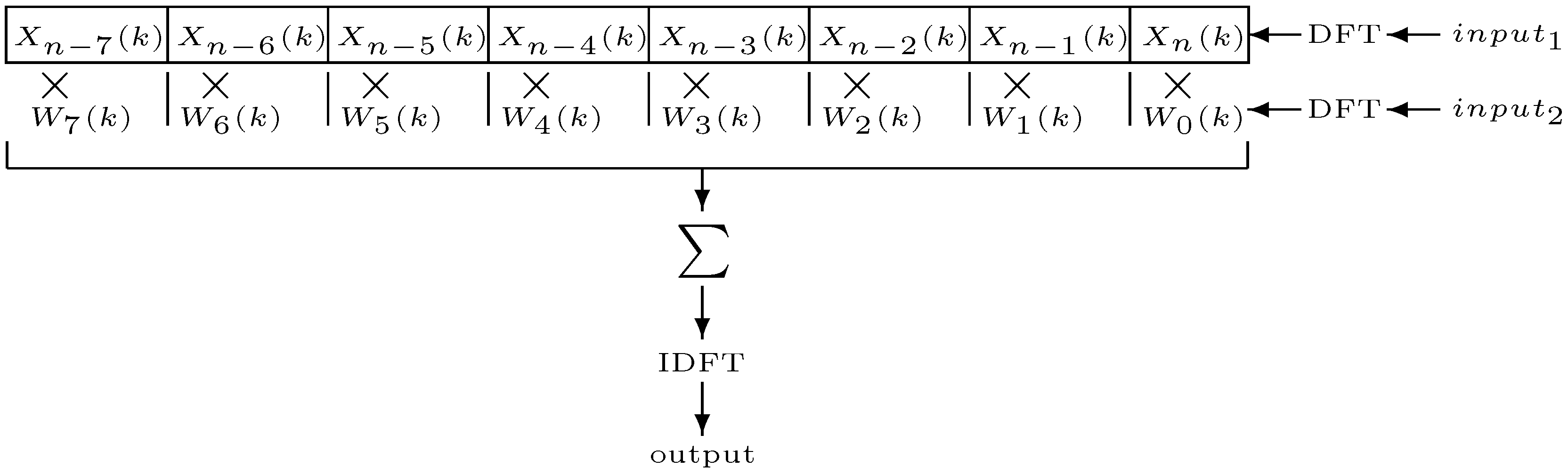
where $w_n\left(m\right)$ is the result of applying a rectangular window of length N to $w\left(n\right)$, localised at time index $n=lN$, with l a non-negative integer, and $\omega =2\pi m/N$. Equally, we can take the input signal DFT,

$$X(n,k)={\displaystyle \sum _{m=0}^{2N-1}}{x}_n\left(m\right)e^{-j\omega k},$$

(25)

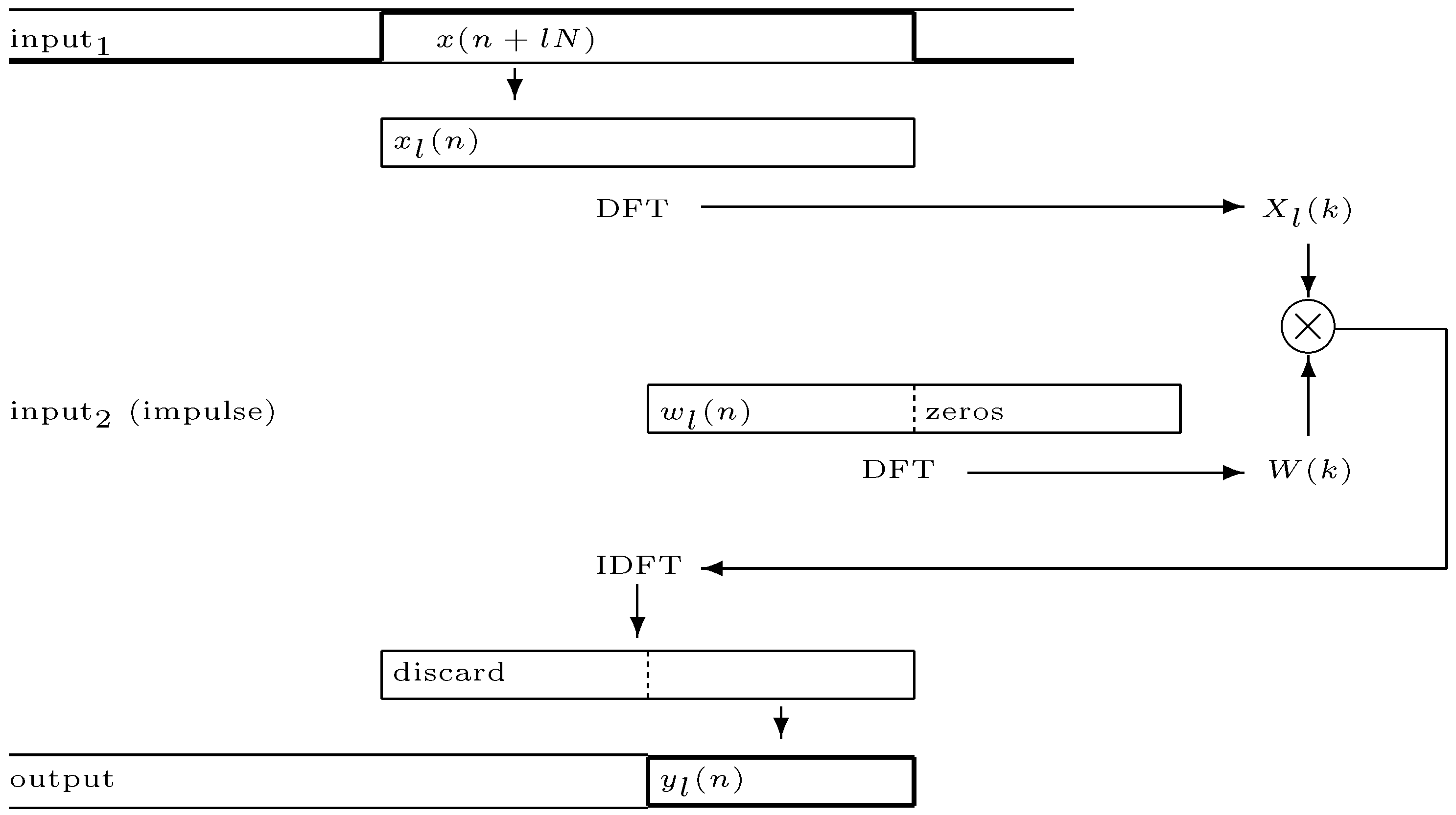
with $x_n\left(m\right)$ similarly defined. The time-varying spectrum of the output of this filter is defined by

$$Y(n,k)=W(n,k)X(n,k).$$

(26)

The resulting spectrum is therefore a sample-by-sample multiplication of the short-time input spectra. The convolution waveform can be obtained by applying an inverse DFT of size $2N$. Therefore, as in the time invariant case, the filter can be implemented either in the time domain with a tapped delay line or in the frequency domain using the fast Fourier transform (FFT).

The time-varying convolution effect is a type of cross-synthesis of two input signals. It tends to emphasise their common components and suppress the ones that are absent in one of them. The size of the filter will have an important role in the extent of this cross-synthesis effect and the amount of time smearing that results. As with this class of spectral processes, there is a trade-off between precise localisation in time and frequency. With shorter filter sizes, the filtering effect is not as distinct, but there is a better time definition in the output. With longer lengths, we observe more of the typical cross-synthesis aspects, but the filter will react more slowly to changes in the input signals.

4.1. Fixing Coefficients

A variation on the time-varying convolution method can be developed by allowing coefficients to be fixed for a certain amount of time. Since there is no particular distinction between the two input signals, it is possible for either of these two to be kept static at any given time. More formally, under these conditions, a given $c_k\left(n\right)$ coefficient update can be described by

$$c_{n\mathrm{mod}\mathrm{N}}=w(n-dN),$$

(27)

where d is a non-negative integer that depends on how long $w\left(n\right)$ is being kept static. If the input signal is varying, we can take that $d=0$. Generally, we can assume that the if signal is held for one full filter period (defined as N samples), then $d=1$. Under these conditions, d would be determined by how many periods the set of coefficients has been static. However, in practice, we can have a more complex sample-by-sample switching that could hold certain coefficients static, while allow others to be updated. In this case, the analysis is not so simple. In an extreme modulation example, we can have coefficients that alternate between delays of $cN$ and $dN$ samples (c and d integer and >0). Again, since there is no distinction between $w\left(n\right)$ and $x\left(n\right)$ in terms of their function in the cross-synthesis process, similar observations apply to the updating of the input signal samples. If we implement sample-by-sample update switches to each input, then we allow a whole range of signal “freezing” effects. Of course, depending on the size of the filter, different results might apply. For example, if we have a long filter, freezing one of the signals will create a short loop that will be applied over and over again to the other input. If the frozen signal is a genuine impulse response, say of a given space, this will work as an ordinary linear time-invariant (LTI) convolution operation. Thus, the TVFIR principles might be applied as a means of switching between different impulse responses. Smooth cross-fading can be implemented as a way of moving from one fixed FIR filter to another using the ideas developed here.

4.2. Test Signals

To illustrate some characteristics of time-varying convolution, we look at some cases of time-varying convolution using test signals as inputs. In the first example, we use a pulse train with a frequency of $f_s/1024$ Hz and a sine wave with frequency of 100 Hz using a filter size equal to 1024 samples. This is shown in Figure 5, where we can see that with a pulse at the start of each new filter, the waveform is reconstructed perfectly. This is of course equivalent to having a fixed IR consisting of a unit sample at the start.

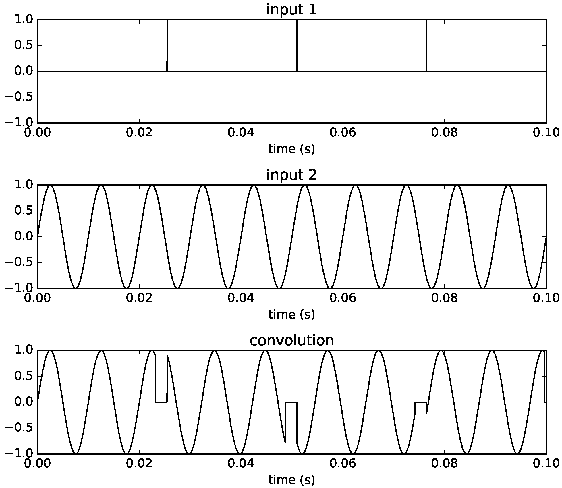
In the second example (Figure 6), we decrease the pulse train frequency to $f_s/1124$ Hz and now the impulses are spaced by 100 more samples than one filter length. The output then contains zeros at these samples, and the sine wave is shifted in time by 100 samples, as the impulse localises the start of the sinusoid at its corresponding time. We can see how the result is that a gap is inserted in the signal.

The final example in Figure 7 shows the converse of this. If we increase the frequency to $f_s/924$ Hz, now a new sinusoid is added to the signal before the previous one has completed its N samples. The effect is to distort the waveform shape at the points where there is an overlap. The distortion appears because the impulses do not coincide with the beginning of the waveform and the waveform itself does not complete full cycles in one filter length.

Note that these examples are somewhat contrived. They are used to illustrate the process of time-varying convolution in a simple way, and are unlikely to arise in practical musical applications of the process. Thus, we need not infer that the quality of cross-synthesis results will be impaired due to the obvious discontinuities seen in the some of the outputs in these examples. However, they are indicative of the fact that the result of the process is very much dependent on the types of inputs as well as the filter lengths employed.

5. Implementation

As noted above, convolution in general can be programmed employing time-domain and/or frequency-domain operations. The trade-off between the two methods are latency between input and output, and efficiency of computation. With an implementation solely using time-domain processing, which we call direct convolution, there is no extra latency imposed by the operation, but we have $O\left(N^2\right)$ complexity. If we implement it in the spectral domain, we can use a radix-2 FFT and reduce the computation demands to $O(NlogN)$, but since we need to wait for all of the N samples of input to be received, we will impose a latency between input and output. This can be compensated for in offline processing but not in real time. However, this latency can be reduced by moving some of the spectral operations to the time domain and reducing the transform size to a fraction of the filter size. This approach is known as partitioned convolution. These ideas are discussed in the remainder of this section.

5.1. Direct Convolution

A time-domain implementation of TVFIR convolution follows closely Equation (23). It employs two delay lines, one for each signal. The rotation in one of the input signals (e.g., $w\left(n\right)$ in Figure 8) to obtain the various coefficients can be simply implemented by looking up the corresponding delay line from end to beginning as if it were a static impulse response. Note that this means that the samples of this signal will always go into the delay line in reverse order. This is conceptually straightforward and the implementation very similar to a standard FIR, except for the fact that we are replacing each sample of the impulse response (as well as feeding a new sample to the delay line holding the other input signal).

5.2. Fast Convolution

Fast convolution employs the fast Fourier transform (FFT) to calculate the DFT, working on blocks of N input samples, with N generally a highly composite number (such as a power-of-two). Two algorithms are more commonly used in frequency domain implementations:

• Overlap-add algorithm (OLA): N samples of each input are collected padded with zeros to make a $2N$ block to which the transforms are applied and their product taken. The output is obtained by taking the inverse FFT of the convolution spectra every N samples. Since this is a $2N$ block of samples, we will need to overlap each output block by N samples (the convolution size is actually $2N-1$ samples, but we expect the last sample of the block to be zero). In a streaming process, this can be achieved by saving the last N samples of the previous output and mixing these with the first N samples from the current one. In this case, we will save the final N samples of the current output as we produce the final overlapped mix. This process is demonstrated in Figure 9.
• Overlap-save algorithm (OLS): $2N$ samples are collected from one of the inputs, and N samples are collected from the other, padded to the filter length. The signals are aligned in such a way that the second half of the first input block corresponds to the start of the second. The products of their spectra is taken and then converted back to the time-domain. The first N samples of this block are discarded, and the second half is output. In a streaming implementation, each iteration will have saved the second half of the last input block (N samples) to use as the first block of the next input to the DFT. A flowchart for this algorithm is shown in Figure 10.
  Since this algorithm depends on the circular property of the DFT, which cannot be guaranteed with a fully time-varying impulse response, it cannot be used in a practical implementation of the TVFIR described by Equations (24)–(26), This is because the OLS algorithm expects that the impulse response data will not vary over the duration of the convolution, which is not the case if both signals are continuously varying. Even in the more restricted scheme of stepwise replacement of impulse responses, the OLS algorithm does not appear to be applicable. With overlapping input blocks, we can no longer assume that the coefficients of the old and new filter are convolved with separate segments of the input signal.

As we noted before, although for longer filter lengths this is the fastest method, we will introduce a latency between input and output that might be objectionable in real-time processing. To mitigate this, the practical solution is to partition the filter size in shorter blocks and apply the process to these, as discussed in the next section.

5.3. Partitioned Convolution

Partitioned convolution attempts to balance computational load and input-output latency. The principle is based on the idea of breaking the filter down into a set of partitions and working in the frequency domain. In the case of time-varying convolution, each input signal is thus segmented and the partitions are converted to the spectral domain and placed in a separate delay line. The products of pairs of partitions (from each input) in the delay line are summed together to produce the spectrum of the convolution (Figure 11). This is converted back to the time domain and overlapped into the output stream, if we are using an overlap-add algorithm, or just output, if using overlap-save.

Conceptually, we can think that direct convolution uses a partition size of one sample, since the DFT of a single sample is an identity operation. As we saw in Section 5.1, this also involves two delay lines, with one of the signals taken in reverse order. The difference here is that to employ partitions bigger than one sample, the operations are performed in the spectral domain. Equally, we can think of fast convolution having partitions of N samples, the filter size, i.e., a single-partition.

5.4. Csound Opcodes

Time-varying convolution has been implemented in Csound [43] in two separate ways, which nevertheless are based on the approaches described in Section 5. The first of these is liveconv, which is an extensive modification of an existing ftconv unit generator. It implements partitioned convolution employing an external function table as a means of sourcing one of the two input signals (nominally the impulse response). The second is tvconv, which takes two audio signal inputs and applies the process for a given filter and partitioned length. In this section, we examine these two implementations in some detail.

5.4.1. liveconv

The liveconv opcode implements dynamic replacement of impulse responses (see Section 3). It employs partitioned convolution with the overlap-add (OLA) scheme. The opcode takes one input signal and a table for holding the impulse response (IR) data:

ares liveconv ain, ift, iplen, kupdate, kclear,

where its parameters are as follows:

• ares: Output signal.
• ain: Input signal.
• ift: Table number for storing the impulse response (IR) for convolution. The table may be filled with new data at any time while the convolution is running.
• iplen: Length of impulse response partition in samples; must be an integer power of two. Lower settings allow for shorter output delay but will increase CPU usage.
• kupdate: Flag indicating whether the IR table should be updated. If kupdate = 1, the IR table ift is loaded partition by partition, starting with the next partition. If kupdate = −1, the IR table ift is unloaded (cleared to zero) partition by partition, starting with the next partition. Other values have no effect.
• kclear: Flag for clearing all internal buffers. If kclear has any value ! = zero, the internal buffers are cleared immediately. This operation is not free of artefacts.

The opcode makes a clear distinction between the input signal $x_1\left(n\right)$ and the IR table. However, if the IR table is updated regularly at filter length: $t_{Rn}=n*N$ and the IR table continuously filled with data from another audio stream $x_2\left(n\right)$, then the inputs $x_1\left(n\right)$ and $x_2\left(n\right)$ will be treated on equal terms, and the opcode behave similar to tvconv without freezing.

The opcode is programmed in C and is available as part of Csound source code [44]. See Algorithm 1 below for pseudocode that highlights the most important parts. For more details, the reader is encouraged to inspect the source code at Github.

Algorithm 1: Liveconv opcode implementation. IR loading marked with blue color.

5.4.2. tvconv

The tvconv opcode takes two input signals and implements time-varying convolution. We can nominally take one of these signals as the impulse response and the other as the input signal, but, in practice, no such distinction is made. The opcode takes the length of the filter and its partitions as parameters, and includes switches to optionally fix coefficients instead of updating them continuously:

asig tvconv ain1, ain2, xupdate1, xupdate2, ipartsize, ifilsize,

where its parameters are as follows:

• ain1, ain2: input signals.
• xupdate1, xupdate2: update switches u for each input signal. If $u=0$, there is no update from the respective input signal, thus fixing the filter coefficients. If $u>0$, the input signal updates the filter as normal. This parameter can be driven from an audio signal, which would work on a sample-by-sample basis, from a control signal, which would work on a block of samples at a time (depending on the ksmps system parameter, the block size), or it can be a constant. Each input signal can be independently frozen using this parameter.
• ipartsize: partition size, an integer P, $0<P\le N$, where N is the filter size. For values $P>1$, the actual partition size will be quantised to $Q=2^k$, $k\in \mathbb{Z}$, $Q\le P$.
• ifilsize: filter size, an integer N, $N\ge P$, where P is the partition size. For partition size values $P>1$, the actual filter size will be quantised to $O=2^k$, $k\in \mathbb{Z}$, $O\le N$.

This opcode is programmed in C++ using the Csound Plugin Opcode Framework (CPOF) [45,46], as the TVConv class. In this code, there are, in fact, two implementations of the process, which are employed according to the partition size:

• For partition size = 1: direct convolution in the time domain is used, and any filter size is allowed. The following method in TVConv implements this (listing 1. The vectors in and ir hold the two delay lines, which take their inputs from the signals in inp and irp. The variables frz1 and frz2 are signals that control the freezing/updating operation for each input.

  Listing 1: Direct convolution implementation.

  int dconv() { csnd::AudioSig insig(this, inargs(0)); csnd::AudioSig irsig(this, inargs(1)); csnd::AudioSig outsig(this, outargs(0)); auto irp = irsig.begin(); auto inp = insig.begin(); auto frz1 = inargs(2); auto frz2 = inargs(3); auto inc1 = csound->is_asig(frz1); auto inc2 = csound->is_asig(frz2); for (auto &s : outsig) { if(*frz1 > 0) *itn = *inp; if(*frz2 > 0) *itr = *irp; itn++, itr++; if(itn == in.end()) { itn = in.begin(); itr = ir.begin(); } s = 0.; for (csnd::AuxMem<MYFLT>::iterator it1 = itn, it2 = ir.end() - 1; it2 >= ir.begin(); it1++, it2--) { if(it1 == in.end()) it1 = in.begin(); s += *it1 * *it2; } frz1 += inc1, frz2 += inc2; inp++, irp++; } return OK; }

• For partition size $>1$, partitioned convolution is used (listing 2), through an overlap-add algorithm. In this case, the process is implemented in the spectral domain, and in order to make it as efficient as possible, power-of-two partition and filter sizes are enforced internally.

  Listing 2: Partitioned convolution implementation.

  int pconv() { csnd::AudioSig insig(this, inargs(0)); csnd::AudioSig irsig(this, inargs(1)); csnd::AudioSig outsig(this, outargs(0)); auto irp = irsig.begin(); auto inp = insig.begin(); auto *frz1 = inargs(2); auto *frz2 = inargs(3); auto inc1 = csound->is_asig(frz1); auto inc2 = csound->is_asig(frz2); for (auto &s : outsig) { if(*frz1 > 0) itn[n] = *inp; if(*frz2 > 0) itr[n] = *irp; s = out[n] + saved[n]; saved[n] = out[n + pars]; if (++n == pars) { cmplx *ins, *irs, *ous = to_cmplx(out.data()); std::copy(itn, itn + ffts, itnsp); std::copy(itr, itr + ffts, itrsp); std::fill(out.begin(), out.end(), 0.); // FFT csound->rfft(fwd, itnsp); csound->rfft(fwd, itrsp); // increment iterators itnsp += ffts, itrsp += ffts; itn += ffts, itr += ffts; if (itnsp == insp.end()) { itnsp = insp.begin(); itrsp = irsp.begin(); itn = in.begin(); itr = ir.begin(); } // spectral delay line for (csnd::AuxMem<MYFLT>::iterator it1 = itnsp, it2 = irsp.end() - ffts; it2 >= irsp.begin(); it1 += ffts, it2 -= ffts) { if (it1 == insp.end()) it1 = insp.begin(); ins = to_cmplx(it1); irs = to_cmplx(it2); // spectral product for (uint32_t i = 1; i < pars; i++) ous[i] += ins[i] * irs[i]; ous[0] += real_prod(ins[0], irs[0]); } // IFFT csound->rfft(inv, out.data()); n = 0; } frz1 += inc1, frz2 += inc2; irp++, inp++; } return OK; }

6. Applications and Use Cases

The two different convolution techniques described above has been used as the basis for two live processing instruments. The instruments are software based and designed to be used with live performers, convolving the sound produced by one musician with the sound produced by another. The instruments are packaged in the form of software plugins in the VST (Virtual Studio Technology (VST) is a software interface that integrates software audio synthesizer and effect plugins with audio editors and recording systems.) plugin format, compiled using the Cabbage [47] framework. Source code for the plugins is available at [48]). This work has been done in the context of a larger research project on crossadaptive audio processing [7], wherein these convolution techniques can be said to form a subset of a larger collection of techniques investigated. The aims of the crossadaptive research forms the motivation for the design of the instruments, and thus it is appropriate to describe these briefly before we move on. It is noteworthy that the work with the application has been done in the context of artistic research, following methods of artistic exploration rather than scientific methods. This means that there have been more of a focus on exploring the unknown potential for creative use of these techniques than there has been on testing explicit hypotheses. Thus, there is not a quantifiable verification of test results, but rather an investigation of some application examples expected to prove useful in our artistic work. Intervention into regular and habitual interaction patterns between musicians is one of the core aspects of the research. More specifically, the project aims to develop and explore various techniques of signal interaction between musical performers, such that the actions of one can influence the sound of the other. This is expected to stir up the habitual interaction patterns between experienced musicians, and thus facilitating novel ways of playing together, enabling new forms of music to emerge. Some of the crossadaptive methods will be intuitive and immediately engaging, others might pose significant challenges for the performers. In many cases, the musical output will not be immediately appealing, as the performers are given an unfamiliar context and unfamiliar tools and instruments. We do still very much rely on their performative experience to solve these challenges, and the instruments are designed to be as playable as possible within the scope and aims outlined. The crossadaptive project includes a wide range of signal interaction models, many based on feature extraction (signal analysis) and mapping the extracted features onto parametric controls of sonic manipulation by means of digital effects processing [49]. Those models of signal interaction has the advantage that any feature can be mapped to any sonic modulation; however, all mappings between features and modulations are also artificial. It is not straightforward to create a set of mappings that is as rich and intuitive to the performer as, for example, the relationship between physical gestures and sonic output of an acoustic instrument.

The convolution techniques that are the focus of this article provide a special case in this regard, as the features of the sound itself contains all aspects of modulation over the other sound. The nuances of the sound to be convolved can be multidimensional and immensely expressive in its features. Still, the performer can use his or her experience in relating the instrumental gestures to the nuances of this sound, which in turn constitute the filter coefficients. Thus, there is a high degree of control intimacy, it is intuitive for the performer to relate performative gestures to sonic output, and, with convolution, the sonic output itself is what modulates the other sound. Relating to the recording of an impulse response is as easy and intuitive for the musician as it is to relate to other kinds of live sampling. These are features of the convolution technique that makes it especially interesting in the context of the crossadaptive performance research. At the same time, the direct and performative live use of convolution techniques also opens the way for a faster and more intuitive exploration of the creative potential of convolution as an expressive sound design tool.

6.1. Liveconvolver

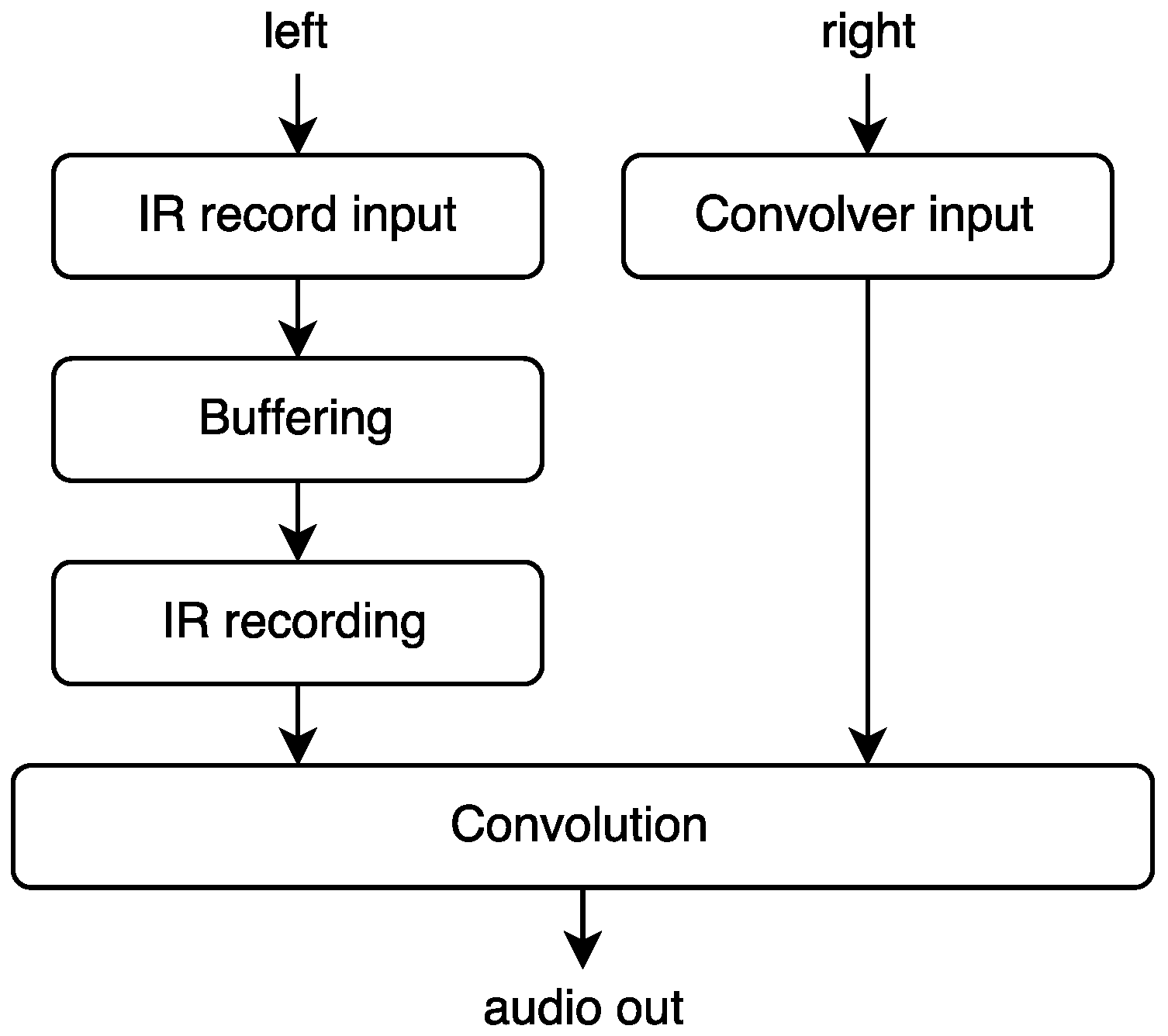
This instrument is designed for convolution of two live signals, but we have retained the concept of viewing one of the signals as an impulse response. This also allows us to retain an analogy with live sampling techniques, as the recording of the impulse response is indeed a form of live capture. The instrument is based on the liveconv opcode as described in Section 5.4.1. The overall signal flow is shown in Figure 12. The audio on the IR record input channel is continuously written to a circular buffer. When we want to replace the current IR, we read from this buffer and replace the IR partition by partition as described under Section 3. The main reason for the circular buffer is to enable transformation (for example time reversal or pitch modification) of the audio before making the IR. If the pitch and direction of the input is not modified, then the extra buffering layer does not impose any extra latency to the process.

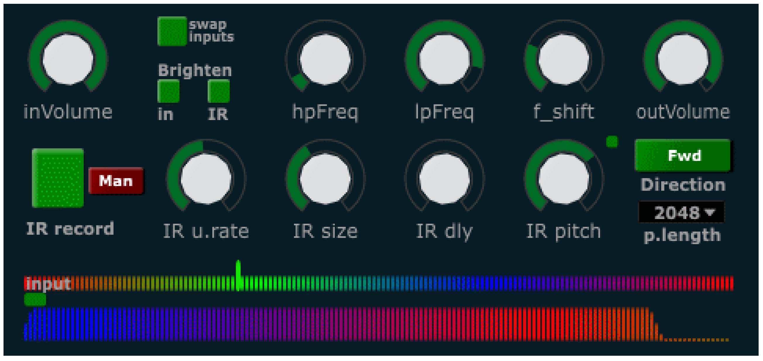
The single most important control of this processing instrument is the trigger for when to replace the IR. This can be done manually via the GUI (Graphical User Interface), see Figure 13, but, for practical reasons, we commonly use an external physical controller or pedal trigger mapped to this switch. One of the musicians then has control over when the IR is updated and how long the new IR will be. In addition to the manual control, this function can also be automatically controlled by means of transient detection or simply set to a periodic update triggered by a metronome. The manual trigger method controlled by an external pedal has been by far the most common use in our experiments.

In addition to the IR record trigger, we have added controls for highpass and lowpass filtering to enable quick adjustments to the spectral profile. When convolving two live signals, the output sound will have a tremendous dynamic range (due to the multiplication of the dynamics of each input sound) and also it will often have a quite unbalanced spectrum (spectral overlap in the two input sounds will be amplified while everything else will be highly attenuated). For this reason, some very coarse and effective controls are needed to shape the output spectrum in a live setting. The described filter controls allows such containment in a convenient manner. Due to the inherent danger of excessive resonances when recording the IR in the same room as the convolver effect is being used, we utilize a simple audio feedback prevention technique (shifting the output spectrum by a few Hz [50] by means of single sideband modulation). This helps in avoiding feedback, but can also be perceived as a subtle detuning. The amount of frequency shift can be adjusted, and, as such, there is a way to minimize the detuning amount for a given performance situation.

Performative Roles with Liveconv

One can distinguish two different performative roles in this kind of interplay: One performer is recording an impulse response (IR), and the other musician plays through the filter created by this IR. It is noteworthy that the two signals are mathematically equivalent in convolution, it does not matter if one convolves sound A with sound B or vice versa, the output sound will be the same (A*B). Still, the two roles facilitates quite different modes of performance, different ways of having control over the output sound. The performer recording the IR will have significant control over the spectral and temporal texture generated, while the musician playing through the filter will have control over the timing and energy flow.

Before starting the practical experimentation, the clarity and implications of these roles were not clear to us. Even so, it was clear that the two musicians would have different roles. The practical sessions would always start with a description of the convolution process and an explanation of how it would affect the sound. Then, each of the musicians would be allowed to perform in both roles, with discussions and reflections in between each take. In the vast majority of experiments, the musical performance was freely improvised, and the musicians was told to just play on the sound coming back to them. The aim was simply to see how they would respond to this new sonic environment and the interaction possibilities presented. The spontaneous and intuitive reaction of skilled performers to this unfamiliar performance scenario was expected to produce something interesting. As artistic exploration, we wanted to keep the possible outcomes as open as possible. There are many variables not explicitly controlled in these experiments. First of all, each musician has a different vocabulary of sounds, phrases, musical reaction patterns and such. Then, the sonic potential and performative affordances of the acoustic instrument being played. Since the resulting sound is a combination of two instruments (and usually two performers), the combinations of above variables affects the output greatly—likewise, the degree to which the musicians knew each other musically before the experiment. The performance conditions in terms of acoustic space, microphone selection and placement, how the processed sound is monitored (speakers, headphones, balance between acoustic and processed sound, etc.), and other external conditions would also potentially affect the output in different ways. If the aim had been to do a scientific investigation of particular aspects (of performance, interaction, timbral modulation, other), these variables would need to be controlled. However, as an artistic exploration of a hitherto unavailable technique, we have opted to keep these things open. The explorative process would thus be open to allow building on preliminary results iteratively, and allow creative input from the participants to affect the course of exploration. The most interesting products of the experiments are the audio recording themselves, as non-exhaustive examples of possible musical uses.

Even if we here identify two distinct performative roles, these were not preconceived but became apparent from noticing similarities between experiments with different musicians. Some musicians in our experiments would prefer the role of playing through the filter, perhaps since it can closely resemble the situation where one is playing through any electronic effect (e.g., an artificial reverb). Others would prefer the role of recording the IR, since this allows the real-time design of the spectrotemporal environment for the other musician to play in. This divide has been apparent in all our practical experiments thus far—for more detail, see, for example, project blog notes about sessions in San Diego [51]). If one, for example, records a single long note as the IR, there is not much to do for the performer playing through the effect other than recreating this tone at different amplitudes. Then, if the impulse response is a series of broadband clicks, this will create a delay pattern and the other musician will have to perform within the musical setting thus constituted.

In spite of the slight imbalance of power, with carefully chosen audio material, both performers can have mutual effect on the output, and the techniques facilitates a closely knitted interplay. In addition, varying the duration of the IR is also an effective way of creating distinctly different sections in an improvisation, and thus can be used to shape formal aspect of the music. Varying the length of the IR also directly affect the power balance between the performative roles: a short IR generally creates a more transparent environment for the other performer to act within. Changing between sustained and percussive sonic material in the IR also has a similar effect, while also retaining a richer image of the temporal activity in the IR recording signal.

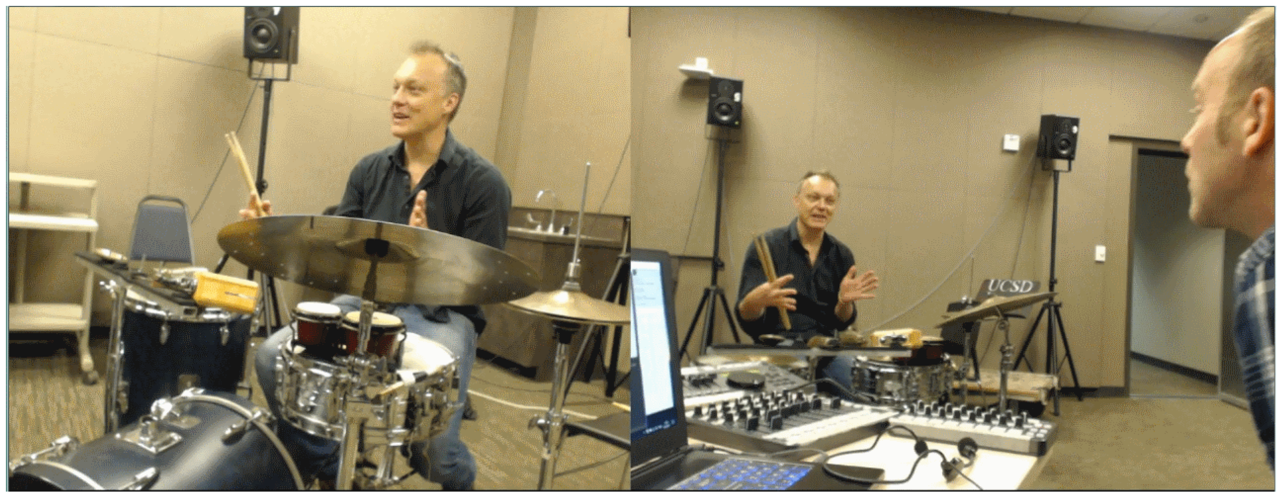
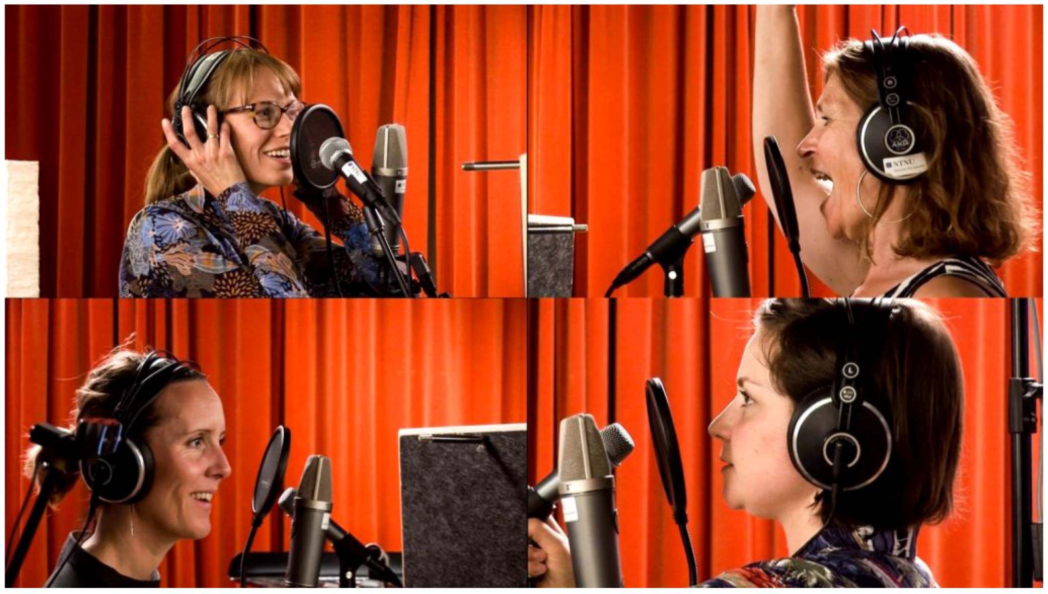
We have experimented with the live convolver technique in studio sessions and concerts since early 2017. There have been sessions in San Diego and Los Angeles (see link in [51] and Figure 14), Oslo (see link in [52], and Trondheim (see link in [53] and Figure 15).

In addition to the creative potential of spectrotemporal morphing, there are also some clear pitfalls. As mentioned, convolution is a multiplicative process, and thus the dynamic range is very large. In addition, it naturally amplifies common frequencies between the two signals, and attenuates everything else. This leads to an unnaturally loud output when the two musicians play melodic phrases where they happen to use common tones. Many musicians will gravitate towards each other’s sound, as a natural aesthetic impulse, trying to create a sonic weave that unites the two sounds. Doing this with live convolution is often counterproductive, as it creates a spectrum with a few extremely high peaks and little other information.

Another danger with live convolution when played over a P.A. in concert is the feedback potential. In this situation, the room (and the sound system) where the performance happens is convolved with itself, effectively multiplying the feedback potential of the system. The performers can also affect the feedback potential, by developing a sensitivity and understanding of which spectral material is most likely to cause feedback problems. Producing material that plays on the resonances of the room generally will increase the danger of feedback. This is another example of a counterintuitive measure for a music performer, as one would normally try to utilize the affordances of the acoustic environment and play things that resonate well in the performance space.

6.2. TV Convolver

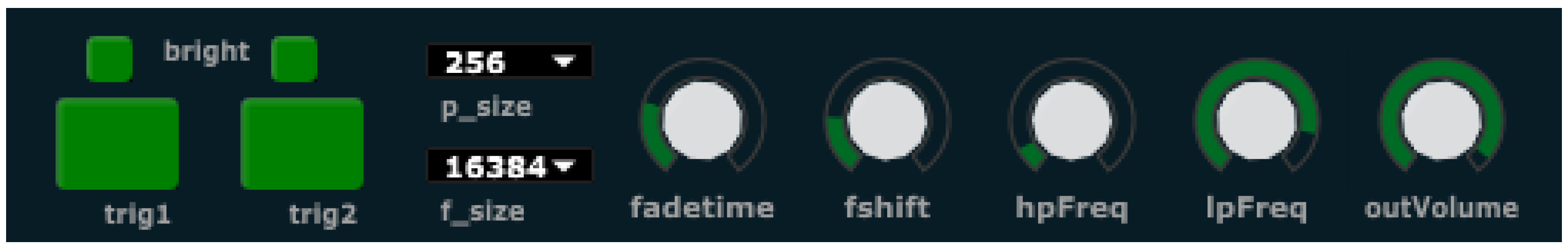
This instrument is designed for convolution of two live signals in a streaming fashion, that is, both signals are treated equally and are continually updated. It is based on the tvconv opcode, as described in Section 5.4.2. It has controls for freezing each of the signals (see Figure 16), that is, bypassing the continuous update of the input buffers. Like the liveconvolver instrument, it also has controls for frequency shift amount (for reduction of feedback potential), highpass and lowpass filtering (for quick adjustment to the output spectrum, see Section 6.1 for details). In addition, it has controls for adjusting the filter length and fade time. The fade time is used in connection with freezing the filter. Even though tvconv allows freezing the filter at any time, we have opted to only allow freezing at filter boundaries, and also to facilitate a fade out of the coefficients towards the boundary when freezing is activated. These measures are done to avoid artefacts due to discontinuities in the filter coefficients. When used with relatively long filter lengths (typically 65,536 samples in our experiments, 1.4 s at a sampling rate of 44.1 kHz), discontinuities due to freezing could be clearly audible as clicks in the audio output. Furthermore, freezing the filter at any arbitrary point would potentially reorder the temporal structure of the live signal used for filter coefficients (see Figure 17 and Figure 18).

Practical Experiments with Tvconv

The streaming nature of this variant of live convolution allows for a constantly changing effect where both of the signals are treated equally. None of them is considered the impulse response for the other to be filtered through; they are simply convolved with each other, where the time window of the convolution is set by the filter length. This instrument has been used in a studio session in Trondheim in August 2017 ([53] and Figure 15), and in several live performances in the weeks and months following the initial studio exploration. Since the two signals are treated equally, there are no technical grounds for assuming different roles for the two performers playing into the effect. This also conforms with our experience.

The effect of tvconv is usually harder to grasp for the performers, compared with the liveconvolver instrument. The interaction between the two signals can be musically counterintuitive. In an improvised musical dialogue, performers will sometimes use a call and response strategy, making a musical statement followed by a pause where other musicians are allowed to respond. With streaming convolution, this is not so productive, since there will be no output unless both input signals are sounding at the same time. Thus, it requires a special performative approach where phrases are interwoven and contrapuntal, with quicker interactions. This manner of simultaneous initiatives could be perceived as aggressive and almost disrespectful in some musical settings, as it might appear as one is trampling all over the other musician’s statements. Negotiating this space of common phrasing very clearly affects the manner in which the musicians can interact, which was one of the objectives of the crossadaptive research project.

Due to the manner in which the filter is updated (see Section 5.4.2), one may perceive a variable latency when performing with tvconv. The technical latency is not variable, but the perceived latency is. This occurs when the first part of the filter contains low amplitude sounds (or sound that is otherwise low in perceptually distinct features), such that the perceived “attack” of the sound is positioned later in the filter (see Figure 19). In this case, one might perceive the filter’s response as having a longer latency than the strictly technical latency of the signal processing. As the filter coefficients are continuously updated in a circular buffer, there is no explicit way of ensuring that perceptually prominent features of the input sound is written to the beginning of the filter. Admittedly, one could argue that a circular buffer does not have a beginning as such, but the way it is used in the convolution process means that it matters where in this buffer salient features of the input sound is positioned. Thus, the perceptual latency can vary within a maximum period set by the size of the filter.

In addition to the immediate interaction of the streaming convolution, another manner of interaction is enabled by giving each of the performers a physical controller (midi pedal) to freeze each of the two filter buffers. If one buffer is frozen, the other performer can play in a more uninterrupted manner, being convolved through the (now static) filter. They can freely switch between freezing one or the other of the inputs and this enables a playful interaction. If both input buffers are frozen, the convolver will output a steady audio loop of length equal to the filter length. In that case, no input is updated, so the filter output is maintained even if both performers fall silent.

We also have a perceptual latency issue when freezing the filter. Since we in our instrument design have allowed freezing only at filter boundaries (see Section 6.2), a signal to freeze the filter does not always freeze the last N seconds (where N is the filter length). Rather, it will continue updating until the write index reaches the filter boundary and then freeze. The time relation between input sounds and the filter buffer is determinate, but since the filter boundaries are not visible or audible to the performers, the relationship will be perceived as somewhat random. In spite of these slight inconveniences, we have focused on the musical use of the filter in performance.

6.3. Demo Sounds

The main application of our convolution techniques has been for live performance. To allow for additional insight into how the processing techniques affect a given source material, we have made some simple demo sounds. These are available online at [54]. The same source have been used for both liveconv and tvconv, and one example output created for each of these two convolution methods. Due to the parametric nature of the methods, a large number of variations on output sounds could be conceived. These two examples simply aim at showing the techniques in their simplest form.

6.4. Future Work

There are some typical problems in using convolution for creative sound design that are even more emphasized when using it for live performance. These relate to the fact that convolution is a multiplicative process, and as such has a tremendous dynamic range. Moreover, if spectral peaks in the two signals overlap, the output sound will tend to have extreme peaks at corresponding frequencies. One possible solution to this might be utilizing a spectral whitening process as suggested by Donahue [55], although this has not yet been fully solved for the case of real-time convolution with time-varying impulse responses. Another approach might be to analyze the two input spectra and selectively reduce the amplitude of overlapping peaks, allowing control over resonant peaks without other spectral modifications. Furthermore, the impulse response update methods described in this article could be applied in more traditional manners, like parametric control of convolution reverbs and so on.

7. Conclusions

The paper has described two new approaches and implementations of time-varying convolution filters. These have been developed in the context of live convolution within improvised electroacoustic performance, as a method of crossmodulation between two audio signals. The implementations has been done in the form of opcodes for the audio programming language Csound. Software instruments for live performance with these opcodes has been built in the form of VST plugins. We have shown some usage examples from studio sessions done within the artistic research project “Cross-adaptive processing as musical intervention”. These practical sessions have also revealed some performative issues and a significant creative potential for further exploration.

References

1. Dolson, M. Recent Advances in Musique Concrète at CARL. In Proceedings of the 1985 International Computer Music Conference, ICMC, Burnaby, BC, Canada, 19–22 August 1985. [Google Scholar]
2. Roads, C. Musical Sound Transformation by Convolution. In Proceedings of the 1993 International Computer Music Conference Opening a New Horizon ICMC, Tokyo, Japan, 10–15 September 1993. [Google Scholar]
3. Truax, B. Convolution Techniques. Available online: https://www.sfu.ca/~truax/Convolution%20Techniques.pdf (accessed on 31 October 2017).
4. Truax, B. Sound, Listening and Place: The aesthetic dilemma. Organ. Sound 2012, 17, 193–201. [Google Scholar] [CrossRef]
5. Moore, A. Sonic Art: An Introduction to Electroacoustic Music Composition; Routledge: London, UK, 2016. [Google Scholar]
6. Gardner, W.G. Efficient Convolution without Input-Output Delay. J. Audio Eng. Soc. 1995, 43, 127–136. [Google Scholar]
7. Brandtsegg, Ø. Cross Adaptive Processing as Musical Intervention; Exploring Radically New Modes of Musical Interaction in Live Performance. Available online: http://crossadaptive.hf.ntnu.no/ (accessed on 7 January 2018).
8. Brandtsegg, Ø.; Saue, S. Live Convolution with Time-Variant Impulse Response. In Proceedings of the 20th International Conference on Digital Audio Effects (DAFx-17), Edinburgh, UK, 5–9 September 2017; pp. 239–246. [Google Scholar]
9. Shmaliy, Y. Continuous-Time Systems; Springer: Heidelberg, Germany, 2007. [Google Scholar]
10. Cherniakov, M. An Introduction to Parametric Digital Filters and Oscillators; John Wiley & Sons: New York, NY, USA, 2003. [Google Scholar]
11. Zetterberg, L.H.; Zhang, Q. Elimination of transients in adaptive filters with application to speech coding. Signal Process. 1988, 15, 419–428. [Google Scholar] [CrossRef]
12. Verhelst, W.; Nilens, P. A modified-superposition speech synthesizer and its applications. In Proceedings of the IEEE International Conference on Acoustics, Speech, and Signal Processing (ICASSP’86), Tokyo, Japan, 7–11 April 1986; Volume 11, pp. 2007–2010. [Google Scholar]
13. Wishnick, A. Time-Varying Filters for Musical Applications. In Proceedings of the 17th International Conference on Digital Audio Effects (DAFx-14), Erlangen, Germany, 1–5 September 2014; pp. 69–76. [Google Scholar]
14. Ding, Y.; Rossum, D. Filter morphing for audio signal processing. In Proceedings of the IEEE ASSP Workshop on Applications of Signal Processing to Audio and Acoustics, New Paltz, NY, USA, 15–18 October 1995; pp. 217–221. [Google Scholar]
15. Zoelzer, U.; Redmer, B.; Bucholtz, J. Strategies for Switching Digital Audio Filters; Audio Engineering Society Convention 95; Audio Engineering Society: New York, NY, USA, 1993. [Google Scholar]
16. Carty, B. Movements in Binaural Space: Issues in HRTF Interpolation and Reverberation, with Applications to Computer Music; Lambert Academic Publishing: Duesseldorf, Germany, 2012. [Google Scholar]
17. Jot, J.M.; Larcher, V.; Warusfel, O. Digital Signal Processing Issues in the Context of Binaural and Transaural Stereophony; Audio Engineering Society Convention 98; Audio Engineering Society: New York, NY, USA, 1995. [Google Scholar]
18. Lee, K.S.; Abel, J.S.; Välimäki, V.; Stilson, T.; Berners, D.P. The switched convolution reverberator. J. Audio Eng. Soc. 2012, 60, 227–236. [Google Scholar]
19. Välimäki, V.; Laakso, T.I. Suppression of transients in variable recursive digital filters with a novel and efficient cancellation method. IEEE Trans. Signal Process. 1998, 46, 3408–3414. [Google Scholar] [CrossRef]
20. Mourjopoulos, J.N.; Kyriakis-Bitzaros, E.D.; Goutis, C.E. Theory and real-time implementation of time-varying digital audio filters. J. Audio Eng. Soc. 1990, 38, 523–536. [Google Scholar]
21. Abel, J.S.; Berners, D. The Time-Varying Bilinear Transform; Audio Engineering Society Convention 141; Audio Engineering Society: New York, NY, USA, 2016. [Google Scholar]
22. Wefers, F.; Vorländer, M. Efficient time-varying FIR filtering using crossfading implemented in the DFT domain. In Proceedings of the 2014 7th Medical and Physics Conference Forum Acusticum, Cracow, Poland, 7–12 September 2014. [Google Scholar]
23. Wefers, F. Partitioned Convolution Algorithms for Real-Time Auralization; Logos Verlag Berlin GmbH: Berlin, Germany, 2015; Volume 20. [Google Scholar]
24. Vickers, E. Frequency-Domain Implementation of Time-Varying FIR Filters; Audio Engineering Society Convention 133; Audio Engineering Society: New York, NY, USA, 2012. [Google Scholar]
25. Settel, Z.; Lippe, C. Real-time timbral transformation: FFT-based resynthesis. Contemp. Music Rev. 1994, 10, 171–179. [Google Scholar] [CrossRef]
26. Wishart, T.; Emmerson, S. On Sonic Art; Contemporary Music Studies; Routledge: New York, NY, USA, 1996. [Google Scholar]
27. Roads, C. Composing Electronic Music: A New Aesthetic; Oxford University Press: Oxford, UK, 2015. [Google Scholar]
28. Engum, T. Real-time Control and Creative Convolution. In Proceedings of the International Conference on New Interfaces for Musical Expression, Oslo, Norway, 30 May–1 June 2011; pp. 519–522. [Google Scholar]
29. Aimi, R.M. Hybrid Percussion: Extending Physical Instruments Using Sampled Acoustics. Ph.D. Thesis, Massachusetts Institute of Technology, Department of Architecture, Program In Media Arts and Sciences, Cambridge, MA, USA, 2007. [Google Scholar]
30. Schwarz, D.; Tremblay, P.A.; Harker, A. Rich Contacts: Corpus-Based Convolution of Contact Interaction Sound for Enhanced Musical Expression. In Proceedings of the International Conference on New Interfaces for Musical Expression, London, UK, 30 June–3 July 2014; pp. 247–250. [Google Scholar]
31. Morris, J.M. Ontological Substance and Meaning in Live Electroacoustic Music. In Genesis of Meaning in Sound and Music, Proceedings of the 5th International Symposium on Computer Music Modeling and Retrieval, Copenhagen, Denmark, 19–23 May 2008; Revised Papers; Ystad, S., Kronland-Martinet, R., Jensen, K., Eds.; Springer: Berlin/Heidelberg, Germany, 2009; pp. 216–226. [Google Scholar]
32. Kagel, M. Transición II; Phonophonie Liner Notes. Available online: http://www.moderecords.com/catalog/127kagel.html (accessed on 4 December 2017).
33. Emmerson, S. Living Electronic Music; Ashgate: Farnham, UK, 2007. [Google Scholar]
34. Casserley, L. A Digital Signal Processing Instrument for Improvised Music. J. Electroacoust. Music 1998, 11, 25–29. [Google Scholar]
35. Oppenheim, A.V.; Schafer, R.W.; Buck, J.R. Discrete-Time Signal Processing, 2nd ed.; Prentice-Hall, Inc.: Upper Saddle River, NJ, USA, 1999. [Google Scholar]
36. Stockham, T.G., Jr. High-speed convolution and correlation. In Proceedings of the Spring Joint Computer Conference ACM, Boston, MA, USA, 26–28 April 1966; pp. 229–233. [Google Scholar]
37. Laroche, J. On the stability of time-varying recursive filters. J. Audio Eng. Soc. 2007, 55, 460–471. [Google Scholar]
38. Lazzarini, V. Computer Music Instruments; Springer: Heildeberg, Germany, 2017. [Google Scholar]
39. Lazzarini, V.; Kleimola, J.; Timoney, J.; Välimäki, V. Five Variations on a Feedback Theme. In Proceedings of the 12th International Conference on Digital Audio Effects, Como, Italy, 1–4 September 2009; pp. 139–145. [Google Scholar]
40. Lazzarini, V.; Kleimola, J.; Timoney, J.; Välimäki, V. Aspects of Second-order Feedback AM synthesis. In Proceedings of the International Computer Music Conference, Huddersfield, UK, 31 July–5 August 2011; pp. 92–98. [Google Scholar]
41. Kleimola, J.; Lazzarini, V.; Välimäki, V.; Timoney, J. Feedback amplitude modulation synthesis. EURASIP J. Adv. Signal Process. 2011, 2011. [Google Scholar] [CrossRef]
42. Timoney, J.; Pekonen, J.; Lazzarini, V.; Välimäki, V. Dynamic Signal Phase Distortion Using Coefficient-Modulated Allpass Filters. J. Audio Eng. Soc. 2014, 62, 596–610. [Google Scholar] [CrossRef]
43. Lazzarini, V.; Ffitch, J.; Yi, S.; Heintz, J.; Brandtsegg, Ø.; McCurdy, I. Csound: A Sound and Music Computing System; Springer: Heidelberg, Germany, 2016. [Google Scholar]
44. Saue, S. Liveconv Source Code. Available online: https://github.com/csound/csound/blob/develop/Opcodes/liveconv.c (accessed on 7 January 2018).
45. Lazzarini, V. The Csound Plugin Opcode Framework. In Proceedings of the 14th Sound and Music Computing Conference 2017, Aalto University, Espoo, Finland, 5–8 July 2017; pp. 267–274. [Google Scholar]
46. Lazzarini, V. Supporting an Object-Oriented Approach to Unit Generator Development: The Csound Plugin Opcode Framework. Appl. Sci. 2017, 7, 970. [Google Scholar] [CrossRef]
47. Walsh, R. Cabbage; A Framework for Audio Software Development. Available online: http://cabbageaudio.com/ (accessed on 7 January 2018).
48. Brandtsegg, Ø. Liveconvolver; Csound Instrument Based around the Liveconvolver Opcode. Available online: https://github.com/Oeyvind/liveconvolver (accessed on 7 January 2018).
49. Brandtsegg, Ø. A Toolkit for Experimentation with Signal Interaction. In Proceedings of the 18th International Conference on Digital Audio Effects (DAFx-15), Trondheim, Norway, 30 November–3 December 2015; pp. 42–48. [Google Scholar]
50. Wigan, E.R.; Alkin, E.G. The BBC Research Labs Frequency Shift PA Stabiliser: A Field Report. BBC Internal Memoranda. 1960. Available online: http://works.bepress.com/edmund-wigan/17/ (accessed on 7 January 2018).
51. Brandtsegg, Ø. Liveconvolver Experiences, San Diego. Available online: http://crossadaptive.hf.ntnu.no/index.php/2017/06/07/liveconvolver-experiences-san-diego/ (accessed on 7 January 2018).
52. Wærstad, B.I. Live Convolution Session in Oslo, March 2017. Available online: http://crossadaptive.hf.ntnu.no/index.php/2017/06/07/live-convolution-session-in-oslo-march-2017/ (accessed on 7 January 2018).
53. Brandtsegg, Ø. Session with 4 Singers, Trondheim, August 2017. Available online: http://crossadaptive.hf.ntnu.no/index.php/2017/10/09/session-with-4-singers-trondheim-august-2017/ (accessed on 7 January 2018).
54. Brandtsegg, Ø. Convolution Demo Sounds. Available online: http://crossadaptive.hf.ntnu.no/index.php/2017/12/07/convolution-demo-sounds/ (accessed on 7 January 2018).
55. Donahue, C.; Erbe, T.; Puckette, M. Extended Convolution Techniques for Cross-Synthesis. In Proceedings of the International Computer Music Conference 2016, Utrecht, The Netherlands, 12–16 September 2016; pp. 249–252. [Google Scholar]
Figure 1. Convolving a time-limited sine sequence with itself.
Applsci 08 00103 g001
Figure 2. Demonstration of dynamic filter replacement: Top: The two filter impulse responses h A ( n ) and h B ( n ) . Bottom: The input signal x ( n ) .
Applsci 08 00103 g002
Figure 3. Demonstration of dynamic filter replacement. Top: The output from convolving the input x ( n ) with impulse response h A ( n ) before n s = 1 s Middle: The output from convolving the input x ( n ) with impulse response h B ( n ) after n s = 1 s Bottom: the output from convolving the input x ( n ) with h A ( n ) and its stepwise with h B ( n ) starting at n s = 1 s The vertical lines mark the time indices n s , n s + N / 3 , n s + 2 N / 3 , and n s + N in the transition region.
Applsci 08 00103 g003
Figure 4. Demonstration of dynamic filter replacement: The content of the filter impulse response buffer at four different points in time: Before transition (1.0 s), 1/3 into the transition (1.5 s), 2/3 into the transition (2.0 s) and after the transition (2.5 s). These time indices are marked with vertical lines in Figure 3.
Applsci 08 00103 g004
Figure 5. Time-varying convolution using a pulse train with frequency f s / 1024 Hz and a sine wave of 100 Hz as inputs, with filter size N = 1024 and sampling rate f s = 44,100.
Applsci 08 00103 g005
Figure 6. Time-varying convolution using a pulse train with frequency f s / 1124 Hz and a sine wave of 100 Hz as inputs, with filter size N = 1024 and sampling rate f s = 44,100.
Applsci 08 00103 g006
Figure 7. Time-varying convolution using a pulse train with frequency f s / 924 Hz and a sine wave of 100 Hz as inputs, with filter size N = 1024 and sampling rate f s = 44,100.
Applsci 08 00103 g007
Figure 8. Direct convolution.
Applsci 08 00103 g008
Figure 9. Fast overlap-add convolution, in this case using two arbitrary time-varying signals.
Applsci 08 00103 g009
Figure 10. Fast overlap-save convolution.
Applsci 08 00103 g010
Figure 11. Partitioned time-varying convolution.
Applsci 08 00103 g011
Figure 12. Liveconvolver instrument flowchart.
Applsci 08 00103 g012
Figure 13. Liveconvolver instrument user interface. As an attempt to visualize when the impulse response is taken from, we use a circular colouring scheme to display the circular input buffer (thin coloured band labeled “input” in the image). We also represent the IR (broader coloured band at the bottom of the image) using the same colours. Time (of the input buffer) is thus represented by colour.
Applsci 08 00103 g013
Figure 14. Kjell Nordeson and Øyvind Brandtsegg discussing live convolver performance.
Applsci 08 00103 g014
Figure 15. Session with singers from Trondheim Voices.
Applsci 08 00103 g015
Figure 16. TV convolver GUI.
Applsci 08 00103 g016
Figure 17. Example of tvconv buffer content when freezing is allowed only at filter boundaries. One contiguous block of audio remains in the filter when frozen.
Applsci 08 00103 g017
Figure 18. Example of tvconv buffer content if freezing is allowed at an arbitrary point. Old content remains in the latter part of the buffer while the first part has been written with new content.
Applsci 08 00103 g018
Figure 19. Impulse response with initial section low on perceptual features, transient occuring later in the filter.
Applsci 08 00103 g019