Article

Surface Roughness Analysis in the Hard Milling of JIS SKD61 Alloy Steel

Department of Mechanical Engineering, National Kaohsiung University of Applied Sciences, 415 Chien Kung Road, Sanmin District, Kaohsiung 80778, Taiwan
*
Author to whom correspondence should be addressed.
Appl. Sci. 2016, 6(6), 172; https://doi.org/10.3390/app6060172
Submission received: 17 April 2016 / Revised: 16 May 2016 / Accepted: 30 May 2016 / Published: 8 June 2016

Abstract

:
Hard machining is an efficient solution that can be used to replace the grinding operation in the mold and die manufacturing industry. In this study, an attempt is made to analyze the effect of process parameters on workpiece surface roughness (Ra) in the hard milling of JIS (Japanese Industrial Standard) SKD61 steel, based on a combination of the Taguchi method and response surface methodology (RSM). The cutting parameters are selected based on the structural dynamic analysis of the machine tool. A set of experiments is designed according to the Taguchi technique. The average Ra is measured by a Mitutoyo Surftest SJ-400, and then analysis of variance (ANOVA) is performed to determine the influences of cutting parameters on the given Ra. Quadratic mathematical modeling is introduced for prediction of the Ra during the hard milling process. The predicted values are in reasonable agreement with the observation of experiments. In an effort to obtain the minimizing Ra, a single objective optimization is employed based on the desirability function. The result shows that the percentage error between measured and predicted values of Ra is 3.2%, which is found to be insignificant. Eventually, the milled surface roughness under the optimized machining conditions is 0.122 µm. This finding shows that grinding may be replaced by finish hard milling in the mold and die manufacturing field.

Graphical Abstract

1. Introduction

JIS SKD61 is a hot-work die steel that is widely used in the mold and die manufacturing industry. It is often utilized to manufacture hot extrusion dies, casting molds, and forging dies due to its significant toughness, high hardness, and sufficient resistance to high temperature fatigue properties. Generally, a mold and die manufacturing process consists of rough machining, heat treatment, and then a finish grinding operation. This process is both costly and time-consuming. Furthermore, the quality of the machined surface produced by the grinding operation is prone to thermal damage [1].
Nowadays, in order to enhance production and product quality in the mold and die manufacturing industry, the finishing grinding process is often replaced by a hard milling operation; this way, the product cycle time can be decreased, productivity increased, and the quality of finished products can be significantly improved [2].
Nevertheless, the JIS SKD61 hardened alloy steel is often acknowledged as a difficult machining material because of its high strength and work hardening rates. Thus, to achieve the best surface quality, highest productivity, and lowest cost, the cutting conditions must be considered and chosen properly whenever hard milling is involved.
Recently, many researchers have effectively applied the Taguchi method to optimize the surface roughness during hard machining processes. For instance, Ding et al. [3] optimized the cutting conditions and developed an experimental equation for surface roughness during milling with (Ti, Al) N-TiN coated inserts of AISI (American Iron and Steel Institute) H13-hardened alloy steel by use of the Taguchi method. The result of their research indicates that the surface roughness under the optimized cutting parameters is less 0.25 µm. Diniz et al. [4] studied the toroidal milling of hardened SAE (Society of Automotive Engineers) H13 alloy steel using the minimum quantity of lubricant (MQL) technique. Their result indicates that the surface roughness value is 0.8 µm. Motorcu [5] used the Taguchi method for optimizing input variables such as cutting speed, feed rate, depth of cut, and tool’s nose radius in the hard turning of AISI 8660 steel with PVD (Physical vapour deposition)-coated ceramic tools. The result reveals that the value of surface roughness is about 1.5 to 2 µm. Asiltürk and Akkuş [6] obtained surface roughness of 1.17 µm under the optimal machining condition during hard turning of AISI 4140 with coated carbide cutting tools.
Furthermore, Dureja et al. [7] optimized the surface roughness during hard turning of AISI H11 steel with TiN coated mixed ceramic insert by RSM. All experiments were designed by use of the Box-Behken method. With optimized machining conditions, they achieve a surface roughness of 0.56 µm. Asiltürk and Neşeli [8] reported the development of a mathematical model and the multiple objective optimization for surface quality when turning AISI 304 steel based on Taguchi and RSM analysis.
On the other hand, many authors have successfully combined RSM with a genetic algorithm (GA) to produce an effective methodology for determining the optimum cutting conditions [9,10,11,12]. They developed experimental models with the RSM and then applied the GA to identify the optimal machining process parameters for the surface finish. With a neural network approach, many researchers have investigated the effects of machining parameters on the surface roughness [13,14].
With most of the researchers mentioned above, the cutting process parameters for hard machining were chosen according to the experience of researchers. They ignored the dynamic parameters of machine tools which significantly affect the surface roughness in machining. Given the nature of these approaches, this did not completely reflect the aspects of machining process.
It is known that the machine tool system is often affected by chatter vibrations during milling operation. The chatter vibrations of the cutting system are generated by a self-excitation phenomenon in the production of chip thickness [15]. In machining, the self-excited machine tool becomes unstable and chatter vibrations grow until the cutter jumps out of the cut [16]. In general, this is one of the common phenomena which negatively affects the machine tool, the cutting tool and the product quality.
Therefore, the analysis of the dynamic parameters of the machine tool system is very important work which needs to be carried out to control the chatter vibration during machining operation. Altintas and Budak [16] analyzed the structural dynamic of the machine tool and developed an analytical model for predicting the chatter vibration of the machine tool system. They noted that the chatter is a self-excited vibration which often occurs in the cutting system as machining with high depths of cut and cutting speed. Thus, they recommended machine tool users for proper selection of depth of cuts and spindle speeds in machining operations. Furthermore, by experimental study, Thamizhmanii et al. [17] showed that the causes of poor surface finish are due to chatter vibrations of a machine tool during machining operation. From the above analysis, it can be seen that the optimal selection of cutting process parameters based on structural dynamic analysis of the machine tool can produce a good surface finish and high performance in machining process.
Moreover, the several studies on the optimal manufacturing process have been performed to minimize cost, improve product quality, and enhance performance through the use of many diverse methods. Unfortunately, each methodology has a different level of efficiency in the computational process. No method has recently provided for the same degree of accuracy within all facets of the machining process.
In order to fill in these gaps, in this study, an attempt has been made to optimize machining process parameters in the hard milling of hardened JIS SKD61 alloy steel with TiAlN coated carbide end mills based on both the Taguchi technique and RSM. The cutting parameters are selected based on the dynamic stability analysis of the machine tool. A series of experiments was designed by use of the Taguchi method. The machined surface profiles are measured by a Surftest SJ-400 (Mitutoyo Corporation, Kanagawa, Japan), and then analysis of variance is carried out by the Minitab 16 package software (Minitab, Inc., Philadelphia, PA, USA, 2010). The influences of cutting conditions such as cutting speed, feed rate, axial depth of cut, and material hardness on Ra are also considered. The second-order model is established to estimate Ra in the hard milling by the RSM. The single objective optimization is carried out to determine the best machining conditions for minimizing Ra.

2. Experimental Details

2.1. Workpiece Material

In this research, the workpiece material was a block of JIS SKD61 alloy steel (Chun Ying Tool Co., Ltd, Changhua, Taiwan) which had the dimensions of 200 mm × 100 mm × 40 mm. The workpiece was through-hardened and tempered to obtain different hardness levels, namely 40, 45, and 50 HRC (Hardness Rockwell C-scale). Their chemical compositions were 0.39% C, 1.0% Si, 0.4% Mn, 5.15% Cr, 1.4% Mo, 0.8% V, and 0.2% Ni [3].

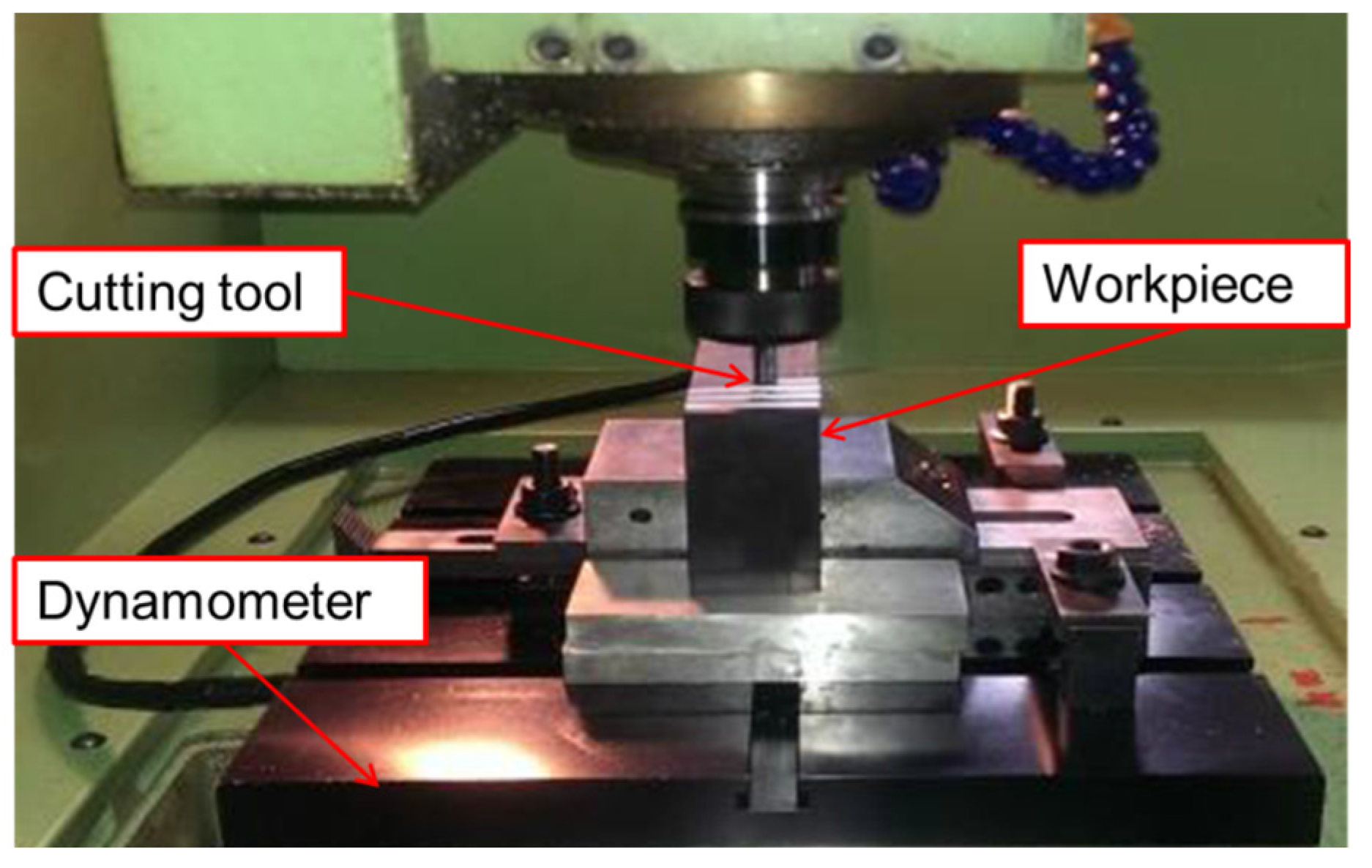
2.2. Tools, Machine Tools and Measurement Instruments

The cutting tools utilized in this study were the TiAlN coated-carbide end mills from CMTec tool manufacturer (Tainan, Taiwan) and their geometry was characterized by: 10 mm diameter, 35 degree helix angle, square type, with 4 flutes. Their cutting ability can reach 60 HRC for the hardened tool steels. The tools were mounted on the machine’s spindle head to carry out the various cutting tasks involved. All the experiments were performed under dry conditions at a Victor V-Center-4 Vertical machining center (Victor Taichung Machinery Works Co., Ltd, Taichung City, Taiwan), which has a maximum spindle speed of 6000 rpm. The workpieces were clamped on the machine table to ensure rigidity during the machining process.

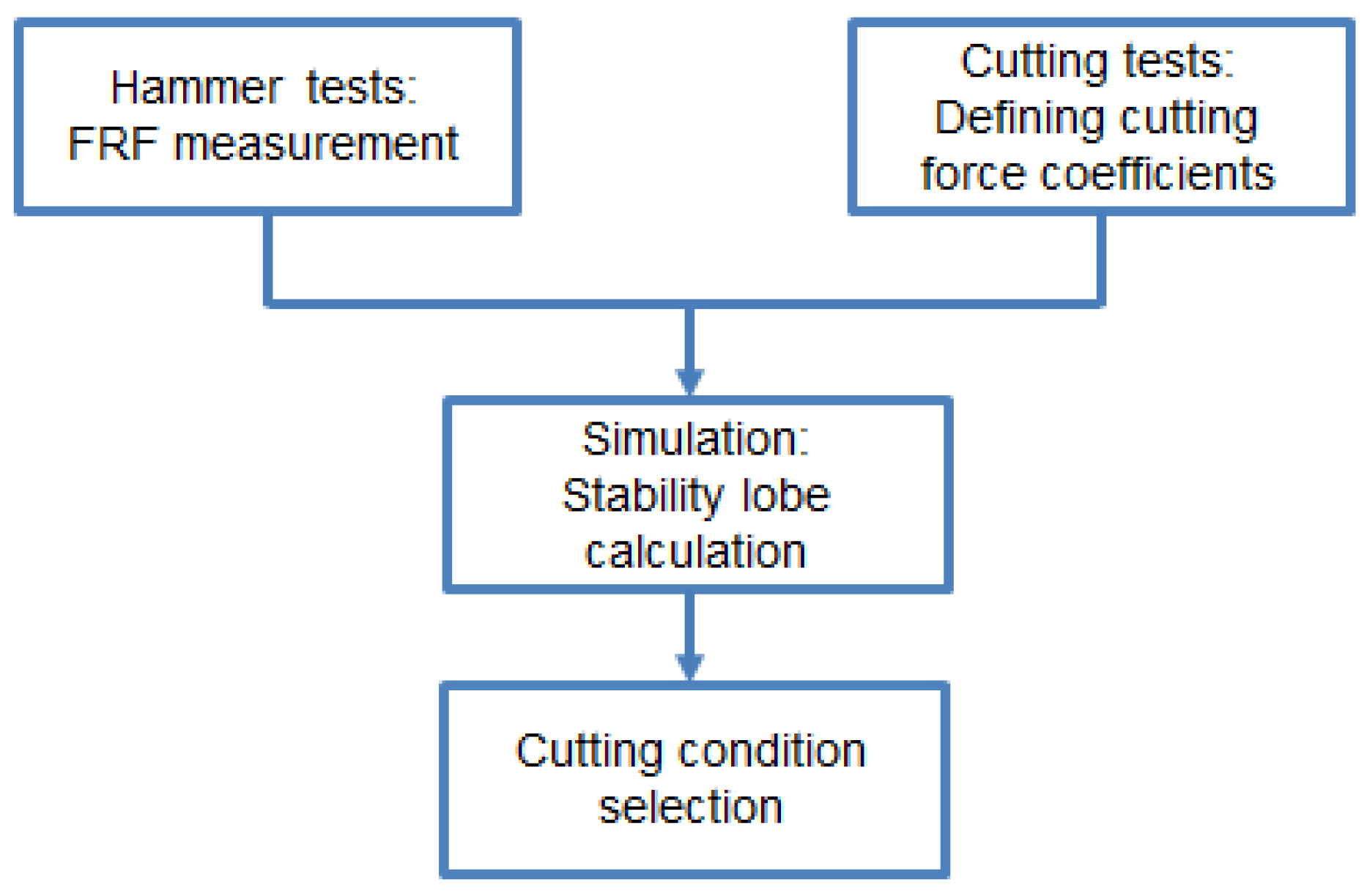
2.3. Identification of Cutting Conditions for the Hard Milling Test

In this study, the cutting conditions for the hard milling test were chosen based on the structural dynamic analysis of a machine tool. The dynamic analysis of the machine tool was performed by use of CUTPRO 9.0 software, 2012. CUTPRO is advanced machining software, which is produced by the Manufacturing Automation Laboratories Corporation in B.C., Canada [18]. It can provide a high efficiency solution for the metal machining field. The procedure of structural dynamic analysis of the machine tool is shown in Figure 1.
First step, the measurements of the machine tool dynamics were carried out by tap testing (hammer test) as illustrated in Figure 2.
From Figure 2, it can be seen that the structural dynamics in both the X and Y directions were measured through the Kistler 9722A2000 Hammer (2.13 mV/N sensitivity) and the 8778A500 M14 Accelerometer (10 mV/g sensitivity) (Kistler Group, Winterthur, Switzerland). The cutting tool was clamped on the machine’s spindle head to carry out the various measurement tasks involved. The accelerometer was mounted on the relief face of the cutter by using a special wax. The output of the accelerometer and the hammer were connected to a PC system. During tap testing, the frequency response functions (FRF) of the structure were measured in two directions by use of the versatile transfer function measurement program in CUTPRO software, which was installed in a PC system.
In the second step, a small series of slotting milling tests were conducted at different feed rates, but constant spindle speed and depth of cut. Furthermore, this study was performed on the hardened JIS SKD61 steel with hardness in the range of (40–50) HRC. Therefore, to ensure machinability, the material which had the highest hardness among given materials was selected to calculate the average cutting force coefficients. With this approach, the input parameters of the average cutting coefficient tests were listed in Table 1 [19]. The procedure of slotting milling tests was shown in Figure 3.
The cutting force components in three directions were measured utilizing a piezoelectric three-component Dynamometer with Model 6423 (Lebow® Products Inc., Troy, MI, USA) and a System 6000’s with Model 6100 scanner (Vishay Precision Group, Inc., Atlanta, GA, USA) connected to a PC employing Strain Smart force measurement software. A digital filter which was designed based on the fast Fourier transform algorithm was integrated into the System 6000 to filter out the noise signal during the measurement. For each machining condition, 1000 data points for each of the three channels were recorded by sampling at 1000 Hz for a period of 1 s.
The modeling of average cutting force coefficients was shown in Equation (1) [15].
K t c = 4 F y c ¯ N a ;   K r c = 4 F x c ¯ N a ;   K a c = π F z c ¯ N a K t e = π F y e ¯ N a ;   K r e = π F x e ¯ N a ;   K a e = 2 F z e ¯ N a
where Ktc, Krc, Kac are cutting coefficients of the tool/workpiece material pairing in tangential, radial and axial directions (N/mm2); Kte, Kre, Kae are edge cutting coefficients of the cutting tool in tangential, radial and axial directions (N/mm); N is the number of teeth on the cutter; a is depth of cut; ( F x c ¯ ,     F y c ¯ ,   F z c ¯ ) and ( F x e ¯ ,     F y e ¯ ,   F z e ¯ ) are average cutting forces and average edge cutting forces in three directions respectively (Newton).
The average cutting force coefficients were calculated from the measured cutting force data obtained through the use of the CUTPRO software. After calculating, the average cutting force coefficients are given in Table 2.
For the third step, once the FRFs and the cutting constants were determined, these data were used in the CUTPRO software to make the stability lobe diagram, as shown in Figure 4. This diagram was produced using Equation (2) [15].
a lim = 2 π Λ R N K t ( 1 + κ 2 )
where a l i m is chatter-free axial depth of cut; N is the number of teeth on the cutter; Kt is the cutting force coefficient; κ = Λ R / Λ I ; Λ R and Λ I are the real part eigenvalue and the imaginary part eigenvalue of the chatter stability equation.
From Figure 4, it was seen that the chatter stability lobes create a spindle speed–dependent dividing line between the unstable and stable depth of cut. These stability lobes can be used to find the best machining parameters for the measured machine tool system.
Finally, the spindle speed and the axial depth of cut in a stable cutting region were selected based upon the chatter stability lobe diagram. From this diagram, the cutting speed (V) in the range of 25–75 m/min and the depth of cut (a) in the range of 0.2–0.6 mm were selected for investigation. Moreover, the present work focused on the study of finish milling of hardened JIS SKD61 alloy steel with hardness in the range of (40–50) HRC. All the experiments were conducted by slotting milling operation. Thus, the best feed rates were often chosen in the range of 0.01–0.03 mm/tooth. The radial depth of cut was seen as a constant that is equal to the diameter of the cutting tool (d = 10 mm). With this approach, the selected cutting condition parameters for hard milling of hardened JIS SKD61 alloy steel are shown in Table 3.

3. Design of Experiments

3.1. Taguchi Technique

The Taguchi technique is a powerful and effective method, which is widely used in the design of experiments and in the optimization of response in engineering fields. In this research work, the Taguchi technique was applied for the design of all the experiments performed. The input variables and its values were given in Table 3. With four three-level factors, Taguchi’s L27 orthogonal array with 27 rows and 13 columns was selected to create a set of tests in the design process [20]. In order to avoid an overlap of the interactions with the main factors, the columns that were chosen are 1, 2, 5, and 12 (see Table 4).

3.2. RSM Based Model for Surface Roughness

According to the ISO 4287 norm, the average surface roughness (Ra) is the arithmetical average of the absolute values of the deviations in the roughness profile from the mean line along the measuring length, as is illustrated in Figure 5. The equation is given for calculating the Ra value as follows [21]:
R a = 1 l 0 l | y ( x ) | d x
where l is the measuring length, and y is the ordinate of the roughness profile.
In this research, the experimental model for predicting the average surface roughness was developed through RSM method. RSM is a statistical and mathematical technique that is often applied to build the empirical model and optimize the input factors (independent variables) for one or more output responses (dependent variables) in the machining process [22].
The relationship between the surface roughness and cutting parameter variables can be expressed by the function as follows [23]:
R a = φ ( V ,   f ,   a , H )
where Ra is the average surface roughness (µm), and V, f, a, and H are the parameters of the cutting speed (m/min), feed (mm/tooth), axial depth of cut (mm) and material hardness (HRC), respectively.
With k input factors, the surface roughness was expressed by the following second-order polynomial function:
R a = β 0 + i = 1 k β i x i + i = 1 k β i i x i 2 + i , j k β i j x i x j + ε  
where xi is coded variables, βi is the coefficient of first-order terms, βii is the coefficient of second-order terms, and βij is the coefficient of interactive terms of the equation.

3.3. Desirability Function

To find the optimal process conditions for output response, numerical optimization was performed using the desirability function. Derringer [24] proposed a multi-objective optimization approach which is considered to be the desirability function. This method is widely applied in engineering to solve inherent multiple objective issues. Each of the responses yi(x) corresponds with a desirability function di(yi) assigning a number in the range from zero to one. One describes the ideal case and zero depicts a condition whereby one or more responses fall outside its acceptable limit. Then, the individual desirability functions are combined by the geometric mean which produces the overall desirability D as follows:
D = ( d 1 × d 2 × d 3 × × d n ) 1 n = ( i = 1 n d i ) 1 n
where n is the number of responses in the measure. If any of the responses are outside their desirable range, the overall function becomes zero.
In order to reflect the possible difference in the importance of each response, Equation (6) can be extended as follows:
D = ( d 1 w 1 × d 2 w 2 × d 3 w 3 × × d n w n )
where wi is weight and satisfies conditions such as 0 < wi < 1 and w1 + w2 + ... + wn = 1.
The numerical optimization is performed to determine a point that represents the maximizing desirability function. Adjustment in importance or weight can change the characteristics of an objective. For many responses, all objectives combine into a desirability function. Each goal is assigned to a response which has low and high values.
The goal of this study is to optimize the input variables for minimizing the surface roughness, so the goal field must be selected as follows:
Minimum:
di = 1 if response < low value
0 ≤ di ≤ 1 as response varies from low to high
di = 0 if response > high value

4. Results and Discussion

In this study, each experiment was repeated three times with a new tool. After experimentation, to obtain statistically significant data for the tests, the workpiece surface roughness was measured at three different positions along the feed direction by a portable surface roughness tester (Surftest SJ-400) with a cut-off length of 2.5 mm and number of cut-offs of 5, and then the average surface roughness was calculated and provided in Table 4. These data were used to analyze the effect of cutting parameters on the surface roughness and to develop the mathematical models used to predict the surface roughness observed in the hard milling process.

4.1. Analysis of Variance for Response Surface

Analysis of variance (ANOVA) is a statistical analysis which is commonly applied to evaluate the data of experiments. In this research, the analysis of direct and interactive effect of the input factors (V, f, a, and H) on the surface roughness is conducted through ANOVA. The regression equation and investigated factors are called to be statistically significant if the p-value in ANOVA Table is less than 0.05. Besides, the percentage contribution (PC) of terms in the estimated model on the total variation is also considered to evaluate the influence degree of the controllable factors on the model.
According to the experimental data in Table 4, the ANOVA for response surface is produced using the Minitab 16 software and their results are further represented in Table 5. Study of these tables indicates that the developed model is found to be statistically significant and is suitable for a Taguchi experiment because of the model’s estimated regression coefficient being (p < 0.0001) less than 0.05 [25]. Moreover, the model terms with a p-value of less than 0.05 reveal that they significantly affect the surface roughness in the investigative range. In such cases, (V), (f), (a), (H), (f2), (V × a) and (f × H) are the statistically significant model terms to be used. Among these terms, the feed rate (f) is the most influential parameter on the Ra which explained 65.33% contribution of total variance. The next effect factor is the depth of cut (a) with a 12.68% contribution. The cutting speed (V), the material hardness (H), and product of the factors such as (f2), (V × a), and (f × H) have little influence on the Ra. Their contributions were 2.97%, 2.66%, 4.88%, 1.39% and 5.24%, respectively. The terms with p-value of more than 0.1 (e.g., V2, a2, H2, V × f, V × H, f × a, and a × H) are not significant, but are not removed from the model to avoid a significant effect on the model’s predictive result [26].
Furthermore, in statistics, R-squared (R2) is called the coefficient of determination for regression analysis that is used to explain the goodness-of-fit of the model to the experimental data. According to ANOVA, the R2 and adjusted R2 value of Ra that are revealed in Table 5 are 0.9645 and 0.9232, respectively. These values are very close to 1. It can be seen that 96.45% of the total variance is justified by the model [26].

4.2. Model of Ra-Based RSM

The quadratic mathematical model, in this research, based on the experimental data, is developed by means of the RSM method for predicting the Ra in the hard milling of JIS SKD61 as follows:
Ra = 0.337 + 0.466 × 10⁻³ × V + 32.505 × f − 0.604 × a − 0.0211 × H − 9.866 × 10⁻⁶ × V2 + 578.333 × f2 − 0.191 × a2 + 0.506 × 10⁻³ × H2 − 0.0502 × V × f + 0.0092 × V × a − 7.155 × 10⁻⁵ × V × H + 7.694 × f × a − 0.977 × f × H + 0.0091 × a × H
The differences between the predicted and the measured values are specified in Figure 6. It shows that there is a good correlation between experimental and predicted results. Thus, the established model is effectively used for predicting Ra in the hard milling of JIS SKD61 alloy steel with 95% confidence intervals.

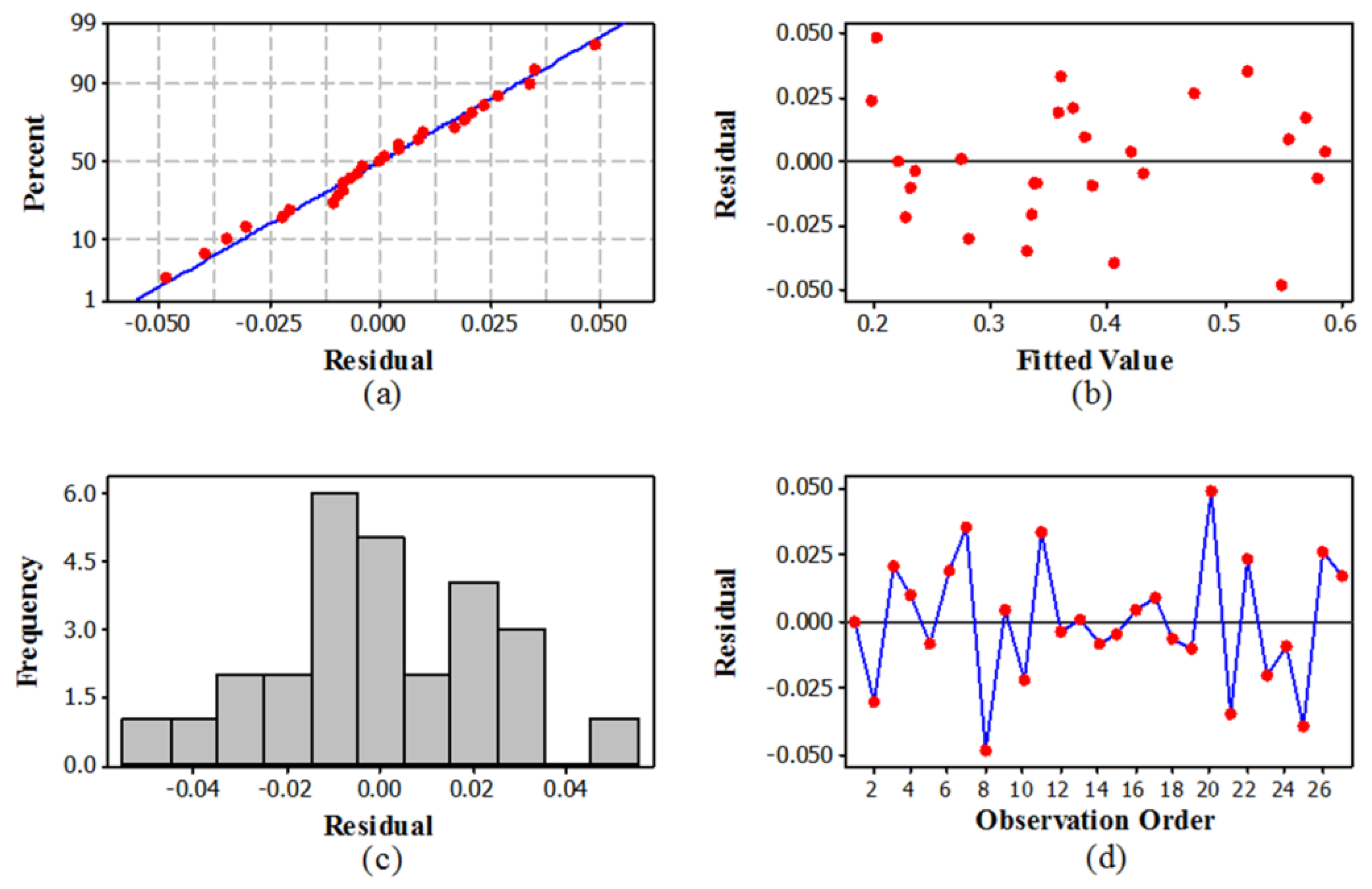
4.3. Verification of Model Adequacy

A model adequacy examination is carried out through residual analysis. It is quite necessary to demonstrate that experimental data are found to be in agreement with the predicted results of the constructed model [26]. All residual plots for surface roughness are indicated in Figure 7. The normal probability plot of residuals in Figure 7a reveals that the residuals are displaced approximately in a straight line, showing that the error distribution is normal and the observed results are in consistent agreement with those of predicted results. This finding is also demonstrated by the plot of the residual versus fitted values in Figure 7b, showing that all values fall within a confidence interval with 95%. It also indicates that the variation between observed values and fitted values is very small [27]. Figure 7c represents the histogram of residuals, which is normally distributed. Figure 7d indicates the residuals and observation order, and it shows that the residuals are independent. Generally, the analysis of residuals reveals that the constructed model is suitable for predicting the surface roughness in hard milling of JIS SKD61 steel, with all residuals falling within control limits [27].

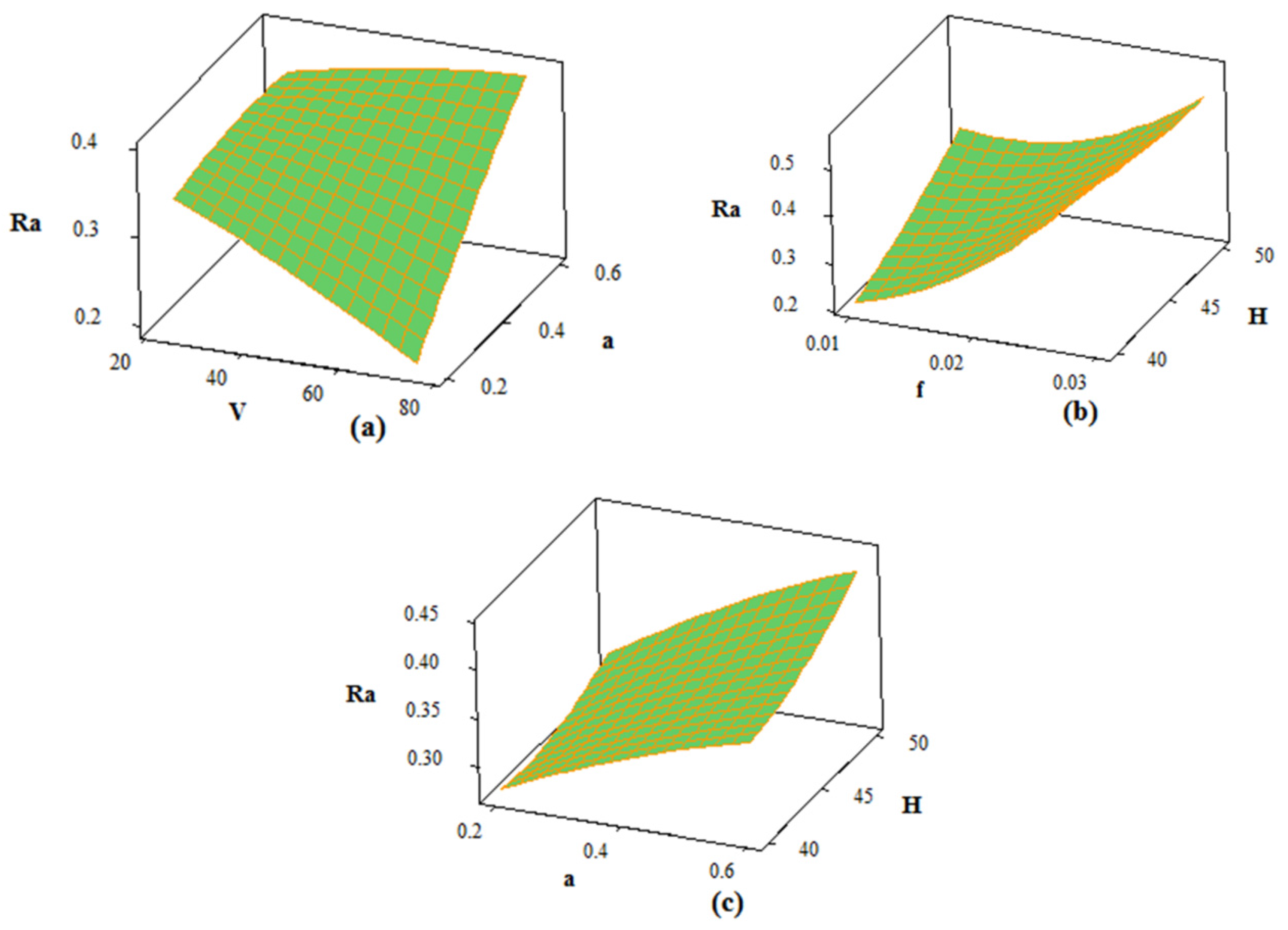
4.4. Interaction Effect of Factors on Response Surface

To clearly understand the interactive influence of independent variables on the response, the 3D surface plots of the Ra are produced based on Equation (8). These graphs are generated according to the change of two factors while remaining factors are seen as a constant, and it is held in the middle level. All plots for the response surface are shown in Figure 8.
Figure 8a indicates the interactive influence of cutting speed (V) and depth of cut (a) on the Ra, for feed rate of 0.02 mm/tooth and material hardness of 45 HRC. This influence is statistically significant (see Table 5). Study of Figure 8a, it shows that the decreasing depth of cut and increasing speed lead to a remarkable decrease in the Ra. This finding is similar to the results achieved by other authors. For instance, Dureja et al. [7] optimized the surface roughness during hard turning of AISI H11 steel with TiN coated mixed ceramic insert by RSM. They concluded that an increase in cutting speed leads to a reduction in the Ra. Çolak et al. [28] predicted the surface roughness in milling process using an evolutionary programming method. They used cutting parameters such as cutting speed, feed and depth of cut to predict the surface roughness. Their results showed that the best surface roughness was always obtained at high cutting speed. This can be explained by the fact that when machining at low speeds, the built-up edge (BUE) is formed on the cutting edge of the tool and will clearly affect the rough surface. However, when the speed is elevated, the BUE breaks away from the cutting edge and hence the machined surface quality becomes better [29]. Moreover, when milling at high cutting speed and low depth of cut, it can cause increased cutting temperatures in the shear zone. This phenomenon will produce a softer workpiece and the chip will be formed easily as a result, so it leads to better surface finish, as reported by Karkalos et al. [30].
Figure 8b specifies the estimated surface roughness in relation to feed rate (f) and material hardness (H), for a cutting speed of 50 m/min and depth of cut of 0.4 mm. From this figure, it can be inferred that the Ra rapidly increases with a corresponding rise in feed rate and material hardness from lower to higher values. It can be explained by the helicoidal movement of tool in machining producing the furrows on machined surfaces. If the feed rate (f) increases in the machining process, the furrows on machined surface will be deeper and broader [31]. Revankar et al. [32] analyzed surface roughness in hard machining of Ti–6Al–4V alloy using PCD (Polycrystalline diamond) tool under different coolant strategies. They concluded that as machining at an increased feed rate, it causes an increase in surface roughness due to less available time to conduct the heat from the machining region, a high material removal rate and an accumulation of chip between the workpiece-cutting tool regions. Hughes et al. [33] analyzed the effect of tool edge preparation on workpiece surface integrity when turning of Ti–6Al–4V alloy. They also indicated that as machining at high feed rate, it results in an increase in surface roughness due to generation of more distinct feed marks.
Figure 8c indicates the influence of depth of cut (a) and material hardness (H) on the Ra, for cutting speed of 50 m/min and feed rate of 0.02 mm/tooth. This plot shows that the surface roughness increases considerably as depth of cut and material hardness increase from lower to higher values. This can be understood that for high material hardness, acceleration of depth of cut provide a chip load which results in an increase in the observable cutting force employed. Several studies have earlier reported that the machined surface quality closely refers to the cutting forces. For instance, Fan and Loftus [34] researched the effect of the cutting forces on machined surfaces. They concluded that the higher cutting forces cause a rougher surface than with the use of smaller cutting forces. Furthermore, Pérez et al. [35] studied the cutting condition for milling of aeronautical alloys. They reported that as machining at high cutting force, it results in chatter vibrations, which leads to an increase in surface roughness. Revankar et al. [32] also revealed that a decrease in the cutting force will lead to a remarkable reduction in the surface roughness as hard turning of Ti–6Al–4V alloy. Colafemina et al. [36] studied the ultra-precision diamond turning of Ti–6Al–4V alloy and developed a relationship between surface roughness and depth of cut. They showed that when machining at low depth of cut, it will result in a drastic reduction in the chatter vibrations.
Compared to the above mentioned researches, our findings also closely agree with the results reported.

4.5. Optimization for Ra

The objective of this research is to find the optimal values of input parameters that minimize Ra when hard milling of JIS SKD61 alloy steel with a coated carbide tool. To solve this problem, the single objective optimization is conducted based on the desirability function. The input parameters, the goals, the limits and the weight are completely listed in Table 6. The results of optimization for the Ra are illustrated in Figure 9 and are also summarized in Table 7.
Table 7 shows that the optimized milling parameters for minimizing Ra are cutting speed of 75 m/min, feed rate of 0.01 mm/tooth, depth of cut of 0.2 mm, a material hardness of 40 HRC and an optimized surface roughness value of 0.118 µm. Moreover, the desirability value is 1 as reported in Table 7. It could be reasonably concluded that the desirability function approach is very suitable for optimizing Ra in machining operations.
Once the optimum machining parameters are determined, the validation experiments need to be carried out to verify the accuracy of the obtained model. The valid result, as shown in Table 7, reveals that the obtained surface roughness Ra under the optimized machining parameters (i.e., V = 75 m/min, f = 0.01 mm/tooth, a = 0.2 mm and H = 40 HRC) is 0.122 µm. The percentage error between measured and predicted values of Ra is 3.2%, which is found to be insignificant. Therefore, the RSM method is considered to be suitable for optimization of surface roughness in the hard milling process of JIS SKD61 steel.
A relative comparison was conducted with other authors. Ding et al. [3] optimized the cutting conditions for surface roughness during milling of AISI H13 hardened alloy steel (equivalent to JIS SKD61 steel). They indicated that the depth of cut was the most influential parameter on the surface roughness. Under the optimized cutting conditions, the surface roughness was less than 0.25 µm. Diniz et al. [4] achieved about 0.8 µm surface roughness value in the toroidal milling of hardened SAE H13. Karkalos et al. [30] obtained 0.19 µm surface roughness value when milling Ti–6Al–4V ELI alloy. They reported that the feed rate and depth of cut have the greatest influence on surface roughness. Cui et al. [37] obtained less than 0.3 µm surface roughness when high-speed face milling AISI H13 steel. They also indicated that the two most important factors affecting the surface roughness were the depth of cut and the cutting speed. However, Vivancos et al. [38] showed that the feed rate was the most effective factor among the given factors on surface roughness when high-speed milling of hardened die steel (61–62) HRC, whereas the cutting speed and the depth of cut were insignificant factors under the same parameters.
The present study shows that the two significantly effective factors on the surface roughness are the feed rate and the depth of cut. This finding is similar to the result obtained from Karkalos et al. [30]. The reason for the effect of feed rate on surface roughness is because the helicoidal movement of tool in machining produces the furrows on machined surfaces [31]. The influence of depth of cut on surface roughness could be due to the surface hardening of alloy steel in hard milling [5].
In this study, the obtained surface roughness value is 0.122 µm. Compared to the above mentioned literature, this research yields a better overall surface roughness result. This is due to the fact that the cutting condition parameters in hard milling of JIS SKD61 alloy steel are properly selected based on the chatter stability diagram of machine tool. Therefore, the workpiece surface roughness is significantly improved.
Normally, the grinding process obtains Ra values from 0.025 µm to 6.3 µm [39]. The milled surface roughness value under optimal cutting conditions is 0.122 µm, which shows that grinding can be replaced by finish hard milling in the mold and die industry.

5. Conclusions

This study presented the optimization of the cutting conditions for Ra when hard milling JIS SKD61 alloy steel (40–50) HRC with coated carbide tool based on a combination of the Taguchi technique and RSM method. Based on this work, conclusions were drawn as follows:
  • Through ANOVA, the results indicate that the control factors such as cutting speed, feed rate, depth of cut, and material hardness have a significant effect on Ra at a reliability level of 95%. The most influential factor on Ra among the investigated factors is the feed rate followed by depth of cut, cutting speed and, finally, material hardness.
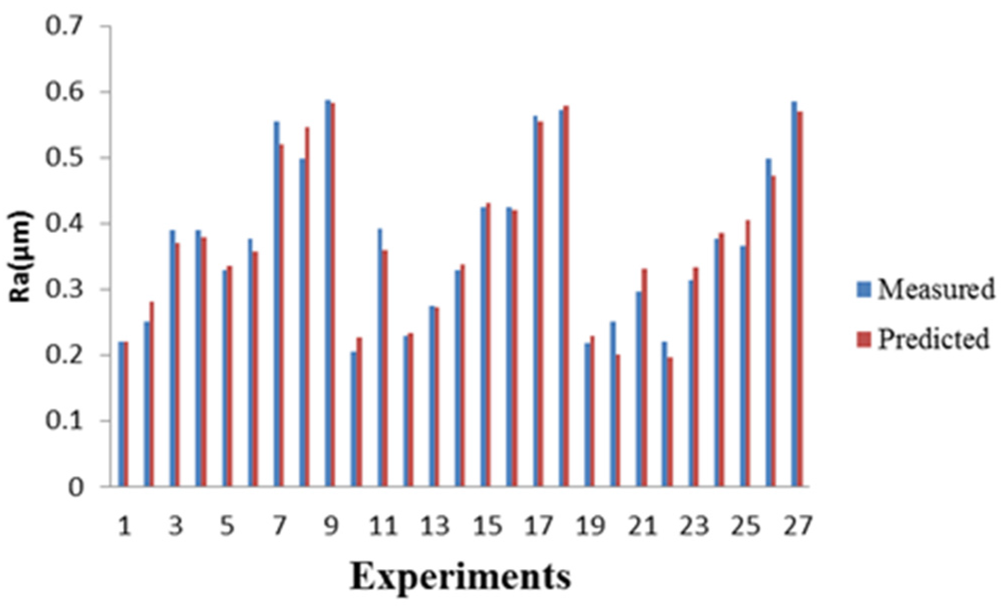
  • According to the response surface analysis, the predicted result of the model is in reasonable alignment with the observations taken from the experiments. Thus, the established model can be utilized to estimate the Ra in the hard milling of JIS SKD61 steel with a 95% confidence interval within the range of machining conditions investigated.
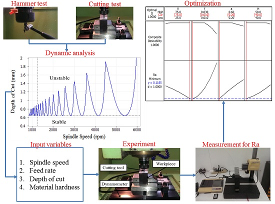
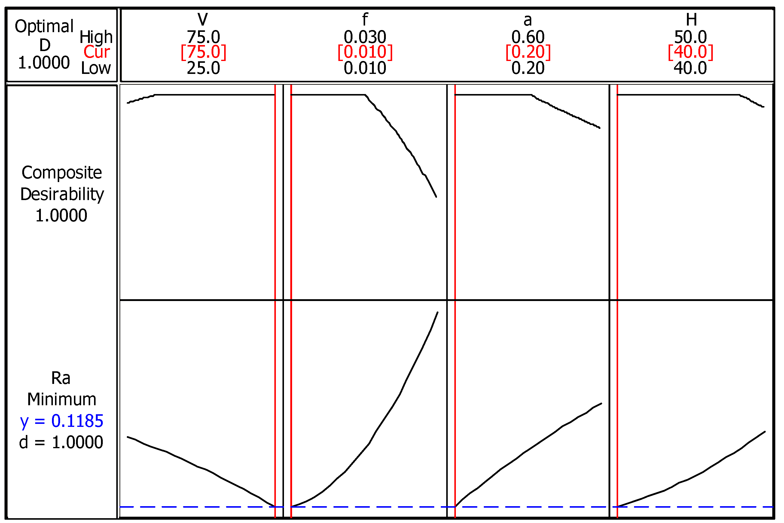
  • The optimized cutting parameters for Ra are a cutting speed of 75 m/min, a feed rate of 0.01 mm/tooth, a depth of cut of 0.2 mm, and material hardness of 40 HRC, with predicted Ra of 0.118 µm.
  • The percentage error between the experimental and predicted values of the minimum Ra is 3.2%, and is found to be insignificant.
  • The milled surface roughness under the optimized machining parameters is 0.122 µm, which can be justified by the fact that the finish hard milling is able to replace the finish grinding in the mold and die manufacturing industry.

Acknowledgments

The authors thank the Department of Mechanical Engineering, and the Department of Mold and Die Engineering of the National Kaohsiung University of Applied Sciences for their instrumental support to insure measurement of surface roughness and the cutting forces required.

Author Contributions

Huu-That Nguyen performed all the cutting experiments, analyzed the data and wrote the paper. Quang-Cherng Hsu developed the research orientation and checked the quality of paper.

Conflicts of Interest

The authors declare no conflict of interest.

References

  1. Zhang, S.; Guo, Y.B. Taguchi method based process space for optimal surface topography by finish hard milling. J. Manuf. Sci. Eng. 2009, 131. [Google Scholar] [CrossRef]
  2. Davim, J.P. Machining of Hard Materials; Springer Science & Business Media: New York, NY, USA, 2011. [Google Scholar]
  3. Ding, T.; Zhang, S.; Wang, Y.; Zhu, X. Empirical models and optimal cutting parameters for cutting forces and surface roughness in hard milling of AISI H13 steel. Int. J. Adv. Manuf. Technol. 2010, 51, 45–55. [Google Scholar] [CrossRef]
  4. Diniz, A.E.; Ferreira, J.R.; Silveira, J.F. Toroidal milling of hardened SAE H13 steel. J. Braz. Soc. Mech. Sci. Eng. 2004, 26, 17–21. [Google Scholar] [CrossRef]
  5. Motorcu, A.R. The optimization of machining parameters using the Taguchi method for surface roughness of AISI 8660 hardened alloy steel. Stroj. Vestnik J. Mech. Eng. 2010, 56, 391–401. [Google Scholar]
  6. Asiltürk, I.; Akkuş, H. Determining the effect of cutting parameters on surface roughness in hard turning using the Taguchi method. Measurement 2011, 44, 1697–1704. [Google Scholar] [CrossRef]
  7. Dureja, J.S.; Gupta, V.K.; Sharma, V.S.; Dogra, M. Design optimization of cutting conditions and analysis of their effect on tool wear and surface roughness during hard turning of AISI-H11 steel with a coated-mixed ceramic tool. Proc. Inst. Mech. Eng. Part B J. Eng. Manuf. 2009, 223, 1441–1453. [Google Scholar] [CrossRef]
  8. Asiltürk, I.; Neşeli, S. Multi response optimisation of CNC turning parameters via Taguchi method-based response surface analysis. Measurement 2012, 45, 785–794. [Google Scholar] [CrossRef]
  9. Öktem, H.; Erzurumlu, T.; Kurtaran, H. Application of response surface methodology in the optimization of cutting conditions for surface roughness. J. Mater. Proc. Technol. 2005, 170, 11–16. [Google Scholar] [CrossRef]
  10. Reddy, N.S.K.; Rao, P.V. A genetic algorithmic approach for optimization of surface roughness prediction model in dry milling. Mach. Sci. Technol. 2005, 9, 63–84. [Google Scholar] [CrossRef]
  11. Reddy, N.S.K.; Rao, P.V. Selection of optimum tool geometry and cutting conditions using a surface roughness prediction model for end milling. Int. J. Adv. Manuf. Technol. 2005, 26, 1202–1210. [Google Scholar] [CrossRef]
  12. Zain, A.M.; Haron, H.; Sharif, S. Application of GA to optimize cutting conditions for minimizing surface roughness in end milling machining process. Expert Syst. Appl. 2010, 37, 4650–4659. [Google Scholar] [CrossRef]
  13. Zain, A.M.; Haron, H.; Sharif, S. Prediction of surface roughness in the end milling machining using Artificial Neural Network. Expert Syst. Appl. 2010, 37, 1755–1768. [Google Scholar] [CrossRef]
  14. Kadirgama, K.; Muhamad, M.N.; Ruzaimi, M.; Rejab, M. Optimization of surface roughness in end milling on mould aluminium alloys (AA6061-T6) using response surface method and radian basis function network. Jordan J. Mech. Ind. Eng. 2008, 2, 209–214. [Google Scholar]
  15. Altintas, Y. Manufacturing Automation: Metal Cutting Mechanics, Machine Tool Vibrations, and CNC Design; Cambridge University Press: Cambridge, UK, 2012. [Google Scholar]
  16. Altintas, Y.; Budak, E. Analytical prediction of stability lobes in milling. CIRP Ann. Manuf. Technol. 1995, 44, 357–362. [Google Scholar] [CrossRef]
  17. Thamizhmanii, S.; Saparudin, S.; Hasan, S. Analyses of surface roughness by turning process using Taguchi method. J. Achiev. Mater. Manuf. Eng. 2007, 20, 503–506. [Google Scholar]
  18. MAL Inc. User Manual for CutPro 9.0; MAL Inc.: Vancouver, BC, Canada, 2012. [Google Scholar]
  19. Taylan, F.; Çolak, O.; Kayacan, M.C. Investigation of TiN coated CBN and CBN cutting tool performance in hard milling application. Stroj. Vestnik J. Mech. Eng. 2011, 57, 417–424. [Google Scholar] [CrossRef]
  20. Ross, P.J. Taguchi Techniques for Quality Engineering; International Editions; Mcgraw-hil: New York, NY, USA, 1996. [Google Scholar]
  21. Arbizu, I.P.; Perez, C.L. Surface roughness prediction by factorial design of experiments in turning processes. J. Mater. Proc. Technol. 2003, 143, 390–396. [Google Scholar] [CrossRef]
  22. Myers, R.H.; Montgomery, D.C. Response Surface Methodology: Process and Product Optimization Using Designed Experiments; Wiley: New York, NY, USA, 2002. [Google Scholar]
  23. Aouici, H.; Yallese, M.A.; Chaoui, K.; Mabrouki, T.; Rigal, J.F. Analysis of surface roughness and cutting force components in hard turning with CBN tool: Prediction model and cutting conditions optimization. Measurement 2012, 45, 344–353. [Google Scholar] [CrossRef]
  24. Derringer, G.; Suich, R. Simultaneous optimization of several response variables. J. Qual. Technol. 1980, 12, 214–219. [Google Scholar]
  25. Esme, U. Surface roughness analysis and optimization for the CNC milling process by the desirability function combined with the response surface methodology. Mater. Test. 2015, 57, 64–71. [Google Scholar] [CrossRef]
  26. Kasim, M.S.; Che Haron, C.H.; Ghani, J.A.; Sulaiman, M.A. Prediction surface roughness in high-speed milling of Inconel 718 under MQL using RSM method. Middle East J. Sci. Res. 2013, 13, 264–272. [Google Scholar]
  27. Palanikumar, K.; Karthikeyan, R. Optimal machining conditions for turning of particulate metal matrix composites using Taguchi and response surface methodologies. Mach. Sci. Technol. 2006, 10, 417–433. [Google Scholar] [CrossRef]
  28. Çolak, O.; Kurbanoğlu, C.; Kayacan, M.C. Milling surface roughness prediction using evolutionary programming methods. Mater. Des. 2007, 28, 657–666. [Google Scholar] [CrossRef]
  29. Jeyakumar, S.; Marimuthu, K.; Ramachandran, T. Prediction of cutting force, tool wear and surface roughness of Al6061/SiC composite for end milling operations using RSM. J. Mech. Sci. Technol. 2013, 27, 2813–2822. [Google Scholar] [CrossRef]
  30. Karkalos, N.E.; Galanis, N.I.; Markopoulos, A.P. Surface roughness prediction for the milling of Ti–6Al–4V ELI alloy with the use of statistical and soft computing techniques. Measurement 2016, 90, 25–35. [Google Scholar] [CrossRef]
  31. Aouici, H.; Bouchelaghem, H.; Yallese, M.A.; Elbah, M.; Fnides, B. Machinability investigation in hard turning of AISI D3 cold work steel with ceramic tool using response surface methodology. Int. J. Adv. Manuf. Technol. 2014, 73, 1775–1788. [Google Scholar] [CrossRef]
  32. Revankar, G.D.; Shetty, R.; Rao, S.S.; Gaitonde, V.N. Analysis of surface roughness and hardness in titanium alloy machining with polycrystalline diamond tool under different lubricating modes. Mater. Res. 2014, 17, 1010–1022. [Google Scholar] [CrossRef]
  33. Hughes, J.I.; Sharman, A.R.C.; Ridgway, K. The effect of tool edge preparation on tool life and workpiece surface integrity. Proc. Inst. Mech. Eng. Part B J. Eng. Manuf. 2004, 218, 1113–1123. [Google Scholar] [CrossRef]
  34. Fan, X.; Loftus, M. The influence of cutting force on surface machining quality. Int. J. Prod. Res. 2007, 45, 899–911. [Google Scholar] [CrossRef]
  35. Pérez, J.; Llorente, J.I.; Sanchez, J.A. Advanced cutting conditions for the milling of aeronautical alloys. J. Mater. Proc. Technol. 2000, 100, 1–11. [Google Scholar]
  36. Colafemina, J.P.; Jasinevicius, R.G.; Duduch, J.G. Surface integrity of ultra-precision diamond turned Ti (commercially pure) and Ti alloy (Ti–6Al–4V). Proc. Inst. Mech. Eng. Part B J. Eng. Manuf. 2007, 221, 999–1006. [Google Scholar] [CrossRef]
  37. Cui, X.; Zhao, J.; Jia, C.; Zhou, Y. Surface roughness and chip formation in high-speed face milling AISI H13 steel. Int. J. Adv. Manuf. Technol. 2012, 61, 1–13. [Google Scholar] [CrossRef]
  38. Vivancos, J.; Luis, C.J.; Ortiz, J.A.; González, H.A. Analysis of factors affecting the high-speed side milling of hardened die steels. J. Mater. Proc. Technol. 2005, 162, 696–701. [Google Scholar] [CrossRef]
  39. Vivancos, J.; Luis, C.J.; Costa, L.; Ortız, J.A. Optimal machining parameters selection in high speed milling of hardened steels for injection moulds. J. Mater. Proc. Technol. 2004, 155, 1505–1512. [Google Scholar] [CrossRef]
Figure 1. Illustrations of the cutting condition selection.
Applsci 06 00172 g001
Figure 2. Dynamic parameter measurement of machine tool.
Applsci 06 00172 g002
Figure 3. Experimental configuration for identification of cutting force coefficients.
Applsci 06 00172 g003
Figure 4. Analytical stability lobe diagram of the hard milling test.
Applsci 06 00172 g004
Figure 5. Graphical representation of roughness parameter Ra.
Applsci 06 00172 g005
Figure 6. The difference between predicted and measured values of Ra.
Applsci 06 00172 g006
Figure 7. Plot of residuals for surface roughness. (a) Normal probability plot of the residuals, (b) residuals versus the fitted values, (c) histogram of the residuals, (d) residuals versus the observation order.
Applsci 06 00172 g007
Figure 8. The response surface plot for Ra. (a) Feed rate of 0.02 mm/tooth, material hardness of 45 HRC, (b) cutting speed of 50 m/min, depth of cut of 0.4 mm, (c) cutting speed of 50 m/min, feed rate of 0.02 mm/tooth.
Applsci 06 00172 g008
Figure 9. Single objective optimization plot.
Applsci 06 00172 g009
Table 1. Experimental conditions for calculating the average cutting force coefficients.
TestSpindle Speed, n (rpm)Feed Rate, f (mm/Tooth)Axial Depth of Cut, a (mm)Hardness, H (HRC)
18500.0500.350
28500.0750.350
38500.1000.350
48500.1250.350
58500.1500.350
Table 2. Average cutting coefficients of JIS SKD61 (50 HRC).
Cutting CoefficientsEdge Cutting Coefficients
Ktc (N/mm2)Krc (N/mm2)Kac (N/mm2)Kte (N/mm)Kre (N/mm)Kae (N/mm)
−654.089−2868.340645.043−66.743−89.74313.832
Table 3. Levels of input variables.
FactorsCode of Levels
123
Cutting speed, V (m/min)255075
Spindle speed, n (rpm)79615922388
Feed rate, f (mm/tooth)0.010.020.03
Axial depth of cut, a (mm)0.20.40.6
Material hardness, H (HRC)404550
Table 4. Experimental results.
Run[1][2][5][12]V (m/min)f (mm/tooth)a (mm)H (HRC)Measured Ra (µm)Predicted Ra (µm)Error (%)
11111250.010.2400.2200.22010.07
21122250.010.4450.2500.280612.2
31133250.010.6500.3900.36935.28
41213250.020.2500.3890.37942.45
51221250.020.4400.3280.33642.59
61232250.020.6450.3760.35724.97
71312250.030.2450.5540.51936.25
81323250.030.4500.4990.54729.67
91331250.030.6400.5880.58390.68
102112500.010.2450.2050.227210.8
112123500.010.4500.3930.35958.51
122131500.010.6400.2300.23401.76
132211500.020.2400.2740.27320.28
142222500.020.4450.3290.33752.60
152233500.020.6500.4250.43011.20
162313500.030.2500.4240.41990.95
172321500.030.4400.5630.55431.53
182332500.030.6450.5720.57891.21
193113750.010.2500.2190.22944.79
203121750.010.4400.2500.201719.3
213132750.010.6450.2960.330611.7
223212750.020.2450.2210.197610.5
233223750.020.4500.3130.33376.62
243231750.020.6400.3760.38552.54
253311750.030.2400.3650.404410.8
263322750.030.4450.4990.47265.27
273333750.030.6500.5860.56902.89
Table 5. Analysis of variance for Ra.
SourceDFSSMSFpPC (%)Remarks
Model140.3958930.02827823.32<0.000196.45Significant
V10.0122200.01222010.080.0082.97Significant
f10.2681560.268156221.2<0.000165.33Significant
a10.0520570.05205742.93<0.000112.68Significant
H10.0109520.0109529.030.0112.66Significant
V210.0002280.0002280.190.6720.05Insignificant
f210.0200680.02006816.550.0024.88Significant
a210.0003530.0003530.290.6000.08Insignificant
H210.0009630.0009630.790.3900.23Insignificant
V × f10.0007680.0014191.170.3010.18Insignificant
V × a10.0057200.01927515.900.0021.39Significant
V × H10.0000190.0007200.590.4560.004Insignificant
f × a10.0021310.0021311.760.2100.51Insignificant
f × H10.0215110.02151117.740.0015.24Significant
a × H10.0007470.0007470.620.4480.18Insignificant
Error120.0145510.001213----
Total260.410444-----
R2 = 0.9645 and adjusted R2 = 0.9232.
Table 6. Constrains and goals for single objective optimization.
ConditionsGoalLower LimitTargetUpper LimitWeight
V (m/min)Is in range25-75-
f (mm/tooth)Is in range0.01-0.03-
a (mm)Is in range0.2-0.6-
H (HRC)Is in range40-50-
Ra (µm)Minimum0.2050.2050.5881
Table 7. The results of the optimization for responses.
ResponsesOptimum ConditionsPredicted ValueExperimental ValueError (%)
V (m/min)f (mm/tooth)a (mm)H (HRC)
Ra (µm)750.010.2400.1180.1223.2
Desirability = 1.

