Disturbance-Resilient Formation Tracking of Tethered Space Net Robots via Distributed Lyapunov-Based MPC

Abstract

Tethered space net robots (TSNRs) offer a flexible and promising configuration for active space debris removal. This study investigates the formation tracking control of TSNR for debris capture in the presence of unknown bounded disturbances. To enhance tracking accuracy, an observer-embedded distributed Lyapunov-based model predictive control (DLMPC) framework is proposed. By integrating real-time estimation errors directly into the predictive model, the framework effectively mitigates the mismatch between predicted and actual system dynamics. In addition, a worst-case contraction constraint is developed to ensure recursive feasibility and robust stability. Numerical experiments demonstrate that the proposed method significantly improves formation tracking precision and enhances resilience against disturbances compared to standard DMPC and auxiliary control strategies.

1. Introduction

Compared with monolithic spacecraft designs, spacecraft swarm systems have become increasingly important in modern space missions due to their superior adaptability and fault tolerance [1]. Distributed control frameworks are increasingly adopted to improve the mission resilience of swarms and mitigate the vulnerabilities associated with centralized schemes [2]. As a prominent swarm configuration, tethered space net robots (TSNR) [3,4] have emerged as a promising solution, particularly suited for capturing space debris and other non-cooperative orbital targets. In a TSNR system, spacecraft are subjected to unpredictable internal forces generated by the deformable tethered net, as well as environmental disturbances such as atmospheric drag, both of which can significantly degrade control performance [5]. At the same time, strict safety distance constraints must be continuously satisfied to ensure collision avoidance among neighboring spacecraft and prevent excessive separation that could cause critical damage to the net [6]. For such systems, achieving high-precision formation tracking while analytically guaranteeing closed-loop robust stability under unknown bounded disturbances and safety constraints remains an open issue.

The tethered net system for capture was first demonstrated in space in the RemoveDEBRIS project [7], where a tethered net was deployed and towed by six passive masses. In contrast to this configuration, the TSNR system relies on four actively maneuvering spacecraft to tow a square tethered net. This distinction significantly enhances autonomous operational flexibility. For uncooperative space targets, the TSNR can adjust the position and orientation of the tethered net during the capture process, leading to enhanced capture performance and reliability [8,9]. However, this highly coupled multi-agent configuration also renders the trajectory tracking control extremely challenging. To address this, Chen et al. introduced an adaptive sliding mode strategy within finite time despite bounded disturbances [5]. In long-distance pursuit scenarios, Ma et al. developed a hierarchical scheme that combines game-theoretic trajectory planning for the leader with a robust adaptive tracking controller for the followers [10]. Although these methods exhibit resilience to disturbances, they often yield sub-optimal trajectories and lack the mechanism to explicitly enforce coupled state constraints, such as safety distances.

Model predictive control (MPC) has gained considerable attention for spacecraft control, as it can optimize control performance under multiple state and input constraints [11,12]. For spacecraft swarm systems, as agent scale and mission complexity increase, distributed MPC (DMPC) formulations are increasingly adopted. These formulations enable cooperative optimization through local information exchange, thereby improving control robustness [13]. Various DMPC-based formation control strategies have been employed for swarm systems [14,15]. In the context of tethered systems, robust DMPC formation tracking control was investigated for transportation via tethered multi-rotor UAVs [16]. In these physically coupled systems, however, classical DMPC methods struggle to provide rigorous theoretical guarantees of closed-loop stability over finite prediction horizons. To overcome this limitation, distributed Lyapunov-based MPC (DLMPC) was proposed. This approach introduces contraction constraints derived from an auxiliary control, ensuring recursive feasibility and closed-loop stability [17,18,19]. For instance, Nie et al. [20] proposed a sequence-scaling DLMPC framework for quadruped robots, while Cui et al. developed a robust spacecraft formation control method based on DLMPC that simultaneously considers both attitude and translational dynamics [21]. Despite its inherent capability for feedback compensation, standard DLMPC often remains insufficient when dealing with significant external disturbances [22]. Consequently, integrating robust anti-disturbance mechanisms into the DLMPC framework becomes essential for maintaining reliable formation control performance.

Several studies have focused on improving robustness within DLMPC-based formation control. For instance, Wei et al. [23] employed an extended state observer to estimate unknown ocean currents, while Jia et al. [24] integrated disturbance observers with prescribed performance control. Long et al. [25] utilized nonlinear backstepping techniques to construct an auxiliary control law to enhance robustness. However, a critical limitation in these existing approaches is that the disturbance estimates are not fully embedded into the prediction model; instead, they are primarily used to enforce stability-related constraints. Consequently, prediction accuracy remains dependent on nominal dynamics, causing deviations between predicted and actual states to accumulate over the horizon. This mismatch often results in conservative control inputs and reduced tracking performance in environments with rapidly varying disturbances.

Motivated by these considerations, this paper proposes an observer-embedded DLMPC algorithm equipped with a worst-case contraction constraint under unknown bounded disturbances. The proposed method aims to achieve optimal formation tracking performance while guaranteeing robust safety for TSNR under disturbances as well as input and state constraints. The main contributions are outlined below:

• A distributed control framework is developed for TSNR system, enabling three-dimensional formation tracking while explicitly handling communication topology, unknown bounded disturbance, and safety constraints induced by the tethered net.
• An observer-embedded prediction mechanism is introduced to mitigate model mismatches and enhance predictive accuracy.
• A worst-case contraction constraint is formulated to account for unknown bounded disturbance within the prediction horizon. Theoretical analysis establishes recursive feasibility and guarantees robust stability of the closed-loop system.

The remainder of this paper is organized as follows. Section 2 formulates the distributed optimization problem, including graph modeling, spacecraft dynamics and constraints. Section 3 introduces the proposed distributed Lyapunov-based MPC framework, encompassing the observer-embedded prediction model, the optimization formulation, and the stability analysis. Simulation studies are provided in Section 4. Finally, Section 5 presents the conclusion.

2. Problem Formulation

This section establishes the mathematical model for formation tracking control problem of the TSNR system, including the directed communication topology, orbital dynamics, the optimization objective and constraints.

2.1. Graph Theory

The communication network among the multiple spacecraft is modeled using graph theory. Consider a system consisting of M spacecraft, each represented as an agent. The collective interaction topology can be described by a graph $\mathcal{G}=(\mathcal{V},\mathcal{E})$, where $\mathcal{V}=\{1,2,\dots ,M\}$ is the finite set of nodes corresponding to the spacecraft. The edge set $\mathcal{E}\subseteq \mathcal{V}\times \mathcal{V}$ defines the communication links between them. In this work, we consider the graph $\mathcal{G}$ to be directed. An edge $(j,i)\in \mathcal{E}$ signifies a unidirectional information flow from spacecraft j to spacecraft i. In this case, spacecraft j is termed a neighbor of spacecraft i. The collection of all neighbors for spacecraft i is represented as ${\mathcal{M}}_i=\{j\in \mathcal{V}:(j,i)\in \mathcal{E}\}$. The adjacency matrix ${\mathit{A}}_{\mathcal{G}}=\left[a_{ij}\right]\in {\mathbb{R}}^{M\times M}$ is a fundamental matrix representation of graph $\mathcal{G}$. Its elements are defined as follows: the diagonal elements are zero, i.e., $a_{ii}=0$ for all $i\in \mathcal{V}$, indicating no self-loops. The off-diagonal elements are given by $a_{ij}=1$ if $(j,i)\in \mathcal{E}$, and $a_{ij}=0$ otherwise.

Assumption 1.

The communication graph $\mathcal{G}$ is assumed to be connected and time-invariant during the operation. Each agent can obtain state information from its neighboring agents defined by the adjacency matrix $A_G$.

2.2. Dynamics Modelling

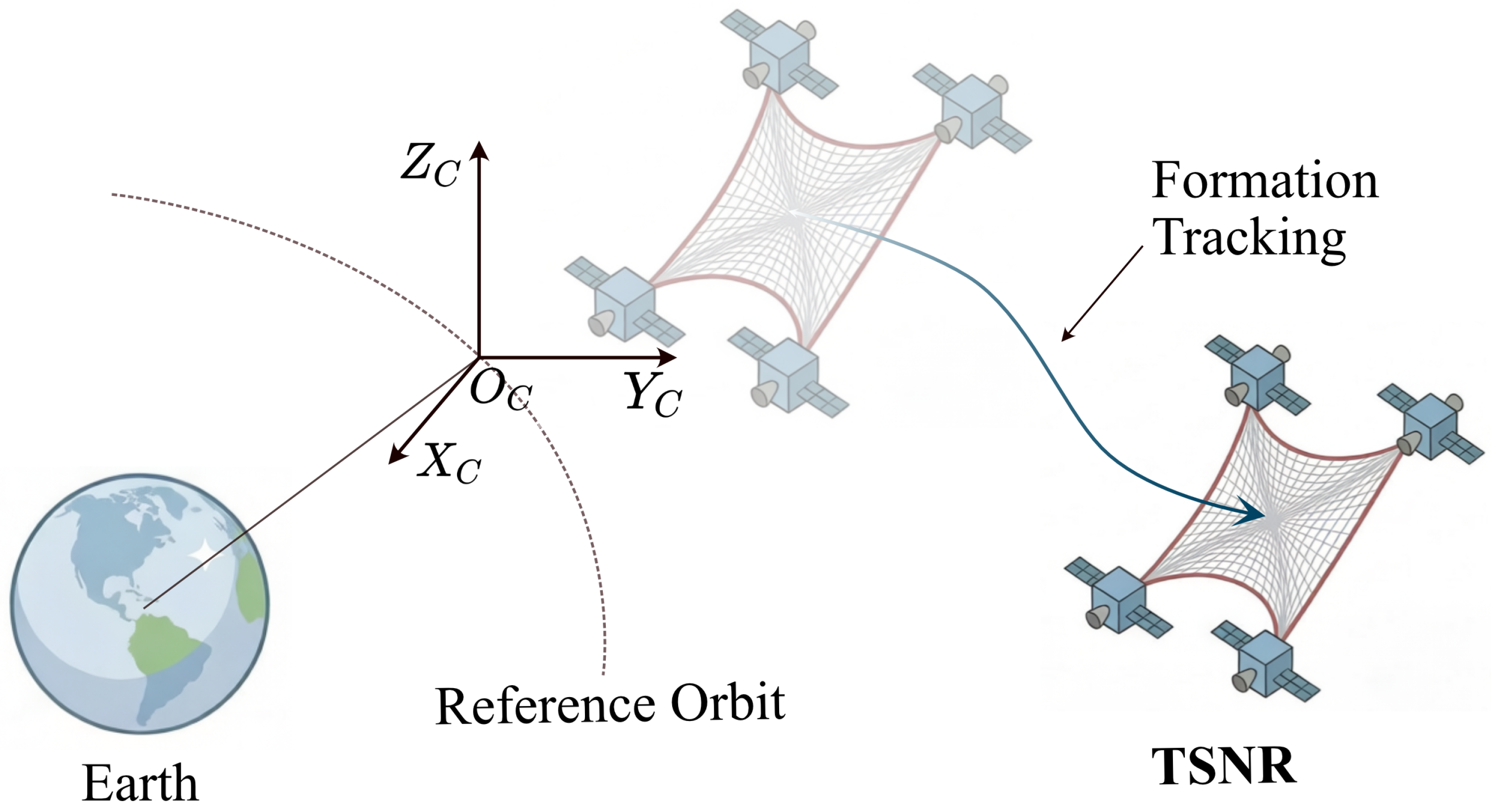
Assuming that the formation tracking control of the TSNR system operates in the close-range capture phase, the relative motion of the spacecraft can be described in the Euler–Hill reference frame, as illustrated in Figure 1. This frame, denoted as $O_c{X}_c{Y}_c{Z}_c$ is oriented with the $X_c$ axis radially outward, the $Z_c$ axis aligned with the angular momentum vector, and the $Y_c$ completing the right-handed orthogonal triad. Then, the relative translational dynamics of the spacecraft in this Euler–Hill reference frame can be described as follows:

$$\begin{array}{cc}\hfill \ddot{x_i}& =3{\omega }_0^2{x}_i+2{\omega }_0{\dot{y}}_i+u_{xi}+f_{xi},\hfill \\ \hfill \ddot{y_i}& =-2{\omega }_0{\dot{x}}_i+u_{yi}+f_{yi},\hfill \\ \hfill \ddot{z_i}& =-{\omega }_0^2{z}_i+u_{zi}+f_{zi},\hfill \end{array}$$

(1)

where ${\omega }_0$ denotes the mean motion of this reference frame, and ${\mathit{u}}_i={[u_{xi},u_{yi},u_{zi}]}^{\top }$ denotes the input of spacecraft i. Considering the physical limitations of the actuators, the control input is restricted by the infinity-norm constraint $\parallel {\mathit{u}}_i{\parallel }_{\infty } \le u_{max}$. ${\mathit{f}}_i={[f_{xi},f_{yi},f_{zi}]}^{\top }$ represents the unknown disturbance vector, capturing both the complex internal tension of the flexible net and external environmental perturbations. The state vector is defined as ${\mathit{x}}_i={[x_i,y_i,z_i,{\dot{x}}_i,{\dot{y}}_i,{\dot{z}}_i]}^{\top }$, which represents the three-dimensional position and velocity of the spacecraft in the reference frame. The dynamic equations can be obtained in the following state-space matrix form:

$${\dot{\mathit{x}}}_i=\widehat{\mathit{A}}{\mathit{x}}_i+\widehat{\mathit{B}}{\mathit{u}}_i+\widehat{\mathit{B}}{\mathit{f}}_i.$$

(2)

The discrete-time system matrices are obtained as follows using the standard zero-order hold discretization, assuming piecewise-constant inputs over each sampling interval.

$${\mathit{x}}_i(k+1)=\mathit{A}{\mathit{x}}_i\left(k\right)+\mathit{B}{\mathit{u}}_i\left(k\right)+\mathit{B}{\mathit{f}}_i\left(k\right),$$

(3)

where $\mathit{A}=e^{\widehat{\mathit{A}}T}$, $\mathit{B}={\int }_0^T{e}^{\widehat{\mathit{A}}t} \mathrm{d}t \widehat{\mathit{B}}$.

Assumption 2.

The unknown disturbances ${\mathit{f}}_i\left(k\right)\in {\mathbb{R}}^3$ acting on each spacecraft i are unknown but norm-bounded, i.e.,

$$\parallel {\mathit{f}}_i{\left(k\right)\parallel }_2\le \overline{f}<\infty ,$$

where $\overline{f}>0$ is a known positive constant. These disturbances encompass both unmodeled internal tether tension forces from the flexible tethered net and external environmental perturbations.

2.3. The Objective of TSNR Formation Control

Consider a desired nominal reference trajectory $\mathit{r}$ for the geometric center of the TSNR system, which can be regarded as the trajectory of a virtual leader. The follower spacecraft exchange information with their neighboring agents and cooperatively achieve formation tracking centered around this virtual leader. The reference state of spacecraft i is defined as ${\mathit{\tau }}_i={\mathit{d}}_i+\mathit{r}$, where ${\mathit{d}}_i$ denotes the desired relative state vector of spacecraft i with respect to the virtual leader. Based on the nominal system model, the corresponding reference control input for spacecraft i can be derived as ${\mathit{u}}_i^n={\widehat{\mathit{B}}}^{-1}\left({\dot{\mathit{\tau }}}_i-\widehat{\mathit{A}}{\mathit{\tau }}_i\right).$ Furthermore, by neglecting the disturbance term ${\mathit{f}}_i$, the reference trajectory in discrete-time form can be obtained from the nominal system dynamics as ${\mathit{\tau }}_i(k+1)=\mathit{A}{\mathit{\tau }}_i\left(k\right)+\mathit{B}{\mathit{u}}_i^n\left(k\right)$.

To achieve formation tracking, the TSNR is required to satisfy the following objectives:

• Trajectory tracking:

  $$\underset{k\to \infty }{lim}\left({\mathit{x}}_i\left(k\right)-\mathit{r}\left(k\right)\right)={\mathit{d}}_i.$$
• Formation maintenance:

  $$\underset{k\to \infty }{lim}\left({\mathit{x}}_i\left(k\right)-{\mathit{x}}_j\left(k\right)\right)={\mathit{d}}_{ij}.$$
• Safety constraints:

  $$\underline{R}\le \parallel {\mathit{x}}_{ij}\left(k\right)\parallel \le \overline{R},$$

where ${\mathit{d}}_{ij}$ denotes the desired relative position between spacecraft i and j, $\underline{R}$ represents the minimum collision-avoidance distance threshold, and $\overline{R}$ denotes the maximum allowable separation distance between spacecraft.

3. Distributed Lyapunov-Based MPC for Formation Tracking

This section proposes a distributed Lyapunov-based MPC approach that achieves robust formation tracking for the TSNR system under unknown bounded disturbances, using observer-embedded disturbance compensation, safety constraints, and a worst-case Lyapunov contraction condition to ensure recursive feasibility and robust stability.

3.1. Observer-Embedded Prediction Model

In practical on-orbit operations, the spacecraft are affected by disturbances, which deteriorate the prediction accuracy if the nominal system dynamics are directly used in the MPC framework. To mitigate this issue, an observer-embedded prediction model is adopted to explicitly offset unknown bounded disturbances in the state evolution. Specifically, for the spacecraft i, an observer is constructed to estimate its system state as

$$\begin{array}{c}\hfill {\mathit{x}}_i^o(k+1)=\mathit{A}{\mathit{x}}_i^o\left(k\right)+\mathit{B}{\mathit{u}}_i\left(k\right)-{\mathit{\zeta }}_{\mathit{i}}\left(k\right),\end{array}$$

(4)

where ${\mathit{x}}_i^o\left(k\right)$ denotes the estimated state and ${\mathit{\zeta }}_{\mathit{i}}\left(k\right)=\mathbf{\Psi }\left({\mathit{x}}_i^e\left(k\right)\right)$ is a correction term designed to suppress the estimation error, which is defined as ${\mathit{x}}_i^e\left(k\right)={\mathit{x}}_i\left(k\right)-{\mathit{x}}_i^o\left(k\right)$.

Motivated by observer-embedded disturbance rejection strategies, the correction signal ${\mathit{\zeta }}_{\mathit{i}}\left(k\right)$ is generated via an auxiliary dynamic system

$$\mathbf{\Psi }:\left\{\begin{array}{cc}\hfill {\mathit{\psi }}_i(k+1)& ={\mathit{A}}_{\psi }{\mathit{\psi }}_i\left(k\right)+{\mathit{B}}_{\psi }{\mathit{x}}_i^e\left(k\right),\hfill \\ \hfill {\mathit{\zeta }}_i\left(k\right)& ={\mathit{C}}_{\psi }{\mathit{\psi }}_i\left(k\right)+{\mathit{D}}_{\psi }{\mathit{x}}_i^e\left(k\right),\hfill \end{array}\right.$$

(5)

where ${\mathit{\psi }}_i\left(k\right)$ is an internal observer state.

Defining the augmented error vector ${\mathit{\chi }}_i\left(k\right)={[{\mathit{x}}_i^e{\left(k\right)}^T,{\mathit{\psi }}_i{\left(k\right)}^T]}^T$, the error dynamics can be compactly expressed as

$${\mathit{\chi }}_i(k+1)={\mathit{A}}_{\mathit{\chi }}{\mathit{\chi }}_i\left(k\right)+{\mathit{B}}_{\mathit{\chi }}{\mathit{f}}_i\left(k\right),$$

(6)

with appropriately defined matrices ${\mathit{A}}_{\mathit{\chi }}=\left[\begin{array}{cc}\mathit{A}+{\mathit{D}}_{\psi }& {\mathit{C}}_{\psi }\\ {\mathit{B}}_{\psi }& {\mathit{A}}_{\psi }\end{array}\right]$, ${\mathit{B}}_{\mathit{\chi }}=\left[\begin{array}{c}\mathit{B}\\ \mathbf{0}\end{array}\right]$. ${\mathit{A}}_{\psi }, {\mathit{B}}_{\psi }, {\mathit{C}}_{\psi }$ and ${\mathit{D}}_{\psi }$ are the design parameters of the observer, which are designed such that all eigenvalues of the matrix $A_{\mathit{\chi }}$ fall within the unit circle in the complex plane (i.e., satisfying the Schur stability condition).

Utilizing the estimated disturbances from the observer, an augmented prediction model is formulated to govern the state evolution within the MPC horizon. For any $n\in \{0,1,\dots ,N-1\}$, the predicted state at the (n + 1)th step can be computed as follows:

$${\tilde{\mathit{x}}}_i(n+1\mid k)=\mathit{A}{\tilde{\mathit{x}}}_i(n\mid k)+\mathit{B}{\tilde{\mathit{u}}}_i(n\mid k)-\mathbf{\Psi }\left({\widehat{\mathit{x}}}_i^e(n\mid k)\right),$$

(7)

where $\tilde{\mathit{x}}(n\mid k)$ represents the prediction of state at time $k+n$ generated at time k. The initial conditions of the prediction model are given by ${\tilde{\mathit{x}}}_i(0\mid k)=x_i\left(k\right)$, and ${\tilde{\mathit{u}}}_i(0\mid k)={\mathit{u}}_i\left(k\right)$. ${\widehat{\mathit{x}}}_i^e(n\mid k)$ is designed as follows:

$${\widehat{\mathit{x}}}_i^e(n\mid k)=\left\{\begin{array}{c}{\mathit{x}}_i^e\left(k\right),\mathrm{for}n=0,\hfill \\ \mathbf{0},\mathrm{otherwise}.\hfill \end{array}\right.$$

(8)

The design of ${\widehat{\mathit{x}}}_i^e(n\mid k)$ aims to align the prediction model with the observer dynamics, which improves trajectory tracking precision. At the initial prediction step ($n=0$), the inclusion of the current estimation error ${\mathit{x}}_i^e\left(k\right)$ ensures consistency between the one-step-ahead predicted state ${\tilde{\mathit{x}}}_i(1\mid k)$ and the observer update ${\mathit{x}}_i^o(k+1)$, effectively eliminating the initial state mismatch. This ensures that the predictive evolution ${\tilde{\mathit{x}}}_i$ starts from a corrected baseline, preventing the accumulation of estimation bias from the very first step of the prediction. For the later steps ($n\ge 1$), the compensation term is omitted. This simplification relies on the assumption that the observer confines the estimation error within a bounded region, making further correction unnecessary in the forward prediction.

3.2. Optimization Formulation

At time instant k, each spacecraft $i\in \mathcal{V}$ solves a finite-horizon optimal control problem, denoted as ${\mathcal{P}}_i$ formulated as follows, to compute its control sequence.

$$\begin{array}{cc}\hfill \underset{{\tilde{\mathit{u}}}_i\left(k\right)}{min}& J_i\left({\mathit{x}}_i\left(k\right),{\tilde{\mathit{u}}}_i\left(k\right),{\mathit{x}}_j^a\left(k\right)\right)\hfill \end{array}$$

(9a)

$$\begin{array}{cc}\hfill \mathrm{s}.\mathrm{t}.& {\tilde{\mathit{x}}}_i(n+1\mid k)=\mathit{A}{\tilde{\mathit{x}}}_i(n\mid k)+\mathit{B}{\tilde{\mathit{u}}}_i(n\mid k)-\mathbf{\Psi }\left({\widehat{\mathit{x}}}_i^e(k+n)\right),\hfill \end{array}$$

(9b)

$$\begin{array}{cc}\hfill & {\tilde{\mathit{x}}}_i(0\mid k)=x_i\left(k\right),\hfill \end{array}$$

(9c)

$$\begin{array}{cc}\hfill & {∥{\tilde{\mathit{u}}}_i\left(n\mid k\right)∥}_{\infty }\le u_{max},\hfill \end{array}$$

(9d)

$$\begin{array}{cc}\hfill & {∥{\mathit{x}}_i(n\mid k)-{\mathit{x}}_j^a(n\mid k))∥}_2\le \overline{R},\forall j\in {\mathcal{N}}_i,\hfill \end{array}$$

(9e)

$$\begin{array}{cc}\hfill & {∥{\mathit{x}}_i(n\mid k)-{\mathit{x}}_j^a(n\mid k))∥}_2\ge \underline{R},\forall j\in {\mathcal{N}}_i,\hfill \end{array}$$

(9f)

$$\begin{array}{cc}\hfill & f_l\left({\tilde{\mathit{u}}}_i(n\mid k)\right)\le 0,\hfill \end{array}$$

(9g)

where ${\mathit{x}}_i\left(k\right)$ denotes the state received from the sensor at time step k, and $u_{max}$ represents the maximum amplitude of the spacecraft actuator. Equations (9e) and (9f) characterize the safety distance constraints between spacecraft and their neighboring agents, ensuring collision avoidance and preventing excessive deformation or damage to the tethered net structure. Furthermore, by evaluating the variation of the corresponding Lyapunov function, the explicit form of the stability constraint in Equation (9g) can be derived. The contraction constraint is formulated to ensure that, under any admissible disturbance realization, the Lyapunov function does not increase when compared to the auxiliary controller.

The formation tracking objective is encoded by penalizing deviations from the desired relative positions with respect to both the global reference and neighboring robots. Neighbor trajectories are approximated using previously optimized control sequences, enabling a distributed implementation without centralized coordination. The stage cost over the prediction horizon is constructed as

$$\begin{array}{cc}\hfill J_i\left({\mathit{x}}_i\left(k\right),{\tilde{\mathit{u}}}_i\left(k\right),{\mathit{x}}_j^a\left(k\right)\right)=\sum _{n=0}^{N-1}\left[\sum _{j\in {\mathcal{N}}_i}\right(& \underset{\mathrm{formation}\mathrm{maintenance}\mathrm{cost}}{\underbrace{a_{ij}{∥{\tilde{\mathit{x}}}_i(n+1\mid k)-{\mathit{x}}_j^a(k+n+1)-{\mathit{d}}_{ij}∥}_{{\mathit{P}}_i}^2}}\hfill \\ \hfill & + \underset{\mathrm{trajectory}\mathrm{tracking}\mathrm{cost}}{\underbrace{a_{0,j}{∥{\tilde{\mathit{x}}}_i(n+1\mid k)-{\mathit{\tau }}_i(n+1\mid k)∥}_{{\mathit{Q}}_i}^2}})\hfill \\ \hfill & +\underset{\mathrm{fuel}\mathrm{consumption}\mathrm{cost}}{\underbrace{{∥{\tilde{\mathit{u}}}_i(n+1\mid k)∥}_{{\mathit{R}}_i}^2}}].\hfill \end{array}$$

(10)

In the above stage cost, ${\mathit{P}}_i$, ${\mathit{Q}}_i$, and ${\mathit{R}}_i$ are symmetric positive definite weighting matrices. The term ${\tilde{\mathit{x}}}_i(n+1\mid k)$ represents the predicted state of spacecraft i, while ${\mathit{x}}_j^a(k+n+1)$, for $j\in {\mathcal{N}}_i$, represents the assumed state of neighboring spacecraft j. The assumed state can be defined as follows:

$${\mathit{x}}_j^a(k+n+1)=\left\{\begin{array}{c}{\tilde{\mathit{x}}}_j^{*}(n+2\mid k-1),n=0,1,\dots ,N-2,\hfill \\ \mathit{A}{\tilde{\mathit{x}}}_j^{*}(k+n),n=N-1,\hfill \end{array}\right.$$

(11)

where ${\mathit{x}}_j^{*}$ denotes the optimal predicted state sequence of spacecraft j.

3.3. Design of Auxiliary Controller

To explicitly guarantee robustness against bounded disturbances, a worst-case contraction constraint is incorporated into the MPC optimization. An auxiliary control law is first introduced as

$${\widehat{\mathit{u}}}_i=-{\mathit{K}}_{{\widehat{\mathit{u}}}_i}({\mathit{\tau }}_i\left(k\right)-{\mathit{x}}_i^o\left(k\right))+{\mathit{u}}_i^n,$$

(12)

where ${\mathit{K}}_{{\widehat{\mathit{u}}}_i}$ represents the auxiliary feedback gain matrix.

A composite Lyapunov function is defined as

$$V_i\left(k\right)={\displaystyle \frac{1}{2}}{\mathit{\chi }}_i{\left(k\right)}^T{\mathit{Q}}_{\mathit{\chi }}{\mathit{\chi }}_i\left(k\right)+{\displaystyle \frac{1}{2}}{\mathit{e}}_i{\left(k\right)}^T{\mathit{Q}}_{\mathit{e}}{\mathit{e}}_i\left(k\right).$$

(13)

In order to achieve both recursive feasibility and robust stability, the worst-case contraction constraint in (9g) is defined by the function $f_l\left({\mathit{u}}_i\left(k\right)\right)$. This function quantifies the maximum possible growth of the Lyapunov function under bounded external disturbances compared to the auxiliary control law. By invoking the Lipschitz continuity of the quadratic Lyapunov function $V_i$ and considering the bounded nature of the disturbance $\parallel {\mathit{f}}_i{\left(k\right)\parallel }_2\le \overline{f}$, the constraint function $f_l$ is constructed to satisfy $V_i(k+1){{|}_{{\mathit{u}}_i}-V_i(k+1)|}_{{\widehat{\mathit{u}}}_i}\le f_l\left({\mathit{u}}_i\left(k\right)\right)$ as follows:

$$\begin{array}{cc}\hfill f_l\left({\mathit{u}}_i\left(k\right)\right)=& \underset{\mathrm{Nominal}\mathrm{Difference}}{\underbrace{{\displaystyle \frac{1}{2}}\left({\overline{\mathit{\xi }}}_{i,k+1}{|}_{{\mathit{u}}_i}^{\top }{\mathit{Q}}_{\overline{\mathit{\xi }}}{\overline{\mathit{\xi }}}_{i,k+1}{|}_{{\mathit{u}}_i}-{\overline{\mathit{\xi }}}_{i,k+1}{{|}_{{\widehat{\mathit{u}}}_i}^{\top }{\mathit{Q}}_{\overline{\mathit{\xi }}}{\overline{\mathit{\xi }}}_{i,k+1}|}_{{\widehat{\mathit{u}}}_i}\right)}}\hfill \\ \hfill & +\underset{\mathrm{Robustness}\mathrm{Margin}}{\underbrace{∥{\overline{\mathit{B}}}_{\overline{\mathit{\xi }}}^{\top }{\mathit{Q}}_{\overline{\mathit{\xi }}}\left({\overline{\mathit{\xi }}}_{i,k+1}{{|}_{{\mathit{u}}_i}-{\overline{\mathit{\xi }}}_{i,k+1}|}_{{\widehat{\mathit{u}}}_i}\right)∥\overline{f}}},\hfill \end{array}$$

(14)

where ${\mathit{Q}}_{\overline{\mathit{\xi }}}=diag({\mathit{Q}}_{\mathit{e}},{\mathit{Q}}_{\mathit{\chi }})$ is the weighting matrix. The term ${\overline{\mathit{\xi }}}_{i,k+1}{|}_{\mathit{u}}$ denotes the predicted nominal composite error state at time $k+1$ starting from the current state ${\mathit{\xi }}_i\left(k\right)$, governed by the following dynamics:

$${\overline{\mathit{\xi }}}_{i,k+1}{|}_{\mathit{u}}=\left[\begin{array}{cc}\mathit{A}& \mathbf{0}\\ \mathbf{0}& {\mathit{A}}_{\mathit{\chi }}\end{array}\right]{\mathit{\xi }}_i\left(k\right)-\left[\begin{array}{c}\mathit{B}\\ \mathbf{0}\end{array}\right](\mathit{u}\left(k\right)-{\mathit{u}}_i^n\left(k\right)).$$

(15)

Here, the composite error state is defined as ${\mathit{\xi }}_i\left(k\right)={[{\mathit{e}}_i{\left(k\right)}^{\top },{\mathit{\chi }}_i{\left(k\right)}^{\top }]}^{\top }$, where ${\mathit{e}}_i\left(k\right)={\mathit{\tau }}_i\left(k\right)-{\mathit{x}}_i\left(k\right)$ represents the formation tracking error, and ${\mathit{\chi }}_i\left(k\right)$ is the disturbance estimation error. The constant matrix ${\overline{\mathit{B}}}_{\overline{\mathit{\xi }}}$ is defined as ${\overline{\mathit{B}}}_{\overline{\mathit{\xi }}}={[-{\mathit{B}}^{\top },{\mathbf{0}}^{\top }]}^{\top }$ to align with the disturbance impact on the error dynamics. While the nominal difference in Equation (14) captures the deterministic effect of the control input, the robustness margin provides a worst-case envelope for the impact of unknown disturbances. By enforcing $f_l\left({\mathit{u}}_i\left(k\right)\right)\le 0$, the optimization ensures that the actual Lyapunov function value under the optimal control ${\mathit{u}}_i$ will not exceed that under the auxiliary law ${\widehat{\mathit{u}}}_i$ for any realization of the disturbance. In addition, the computational flow for optimizing each spacecraft based on the proposed method is illustrated in Algorithm 1.

Algorithm 1 Observer-Embedded DLMPC Implementation for TSNR Formation

Initialization:  For each spacecraft $i\in \mathcal{V}$, set sampling period $\Delta t$, horizon N, and weights ${\mathit{P}}_i,{\mathit{Q}}_i,{\mathit{R}}_i$;  Define observer matrices $({\mathit{A}}_{\psi },{\mathit{B}}_{\psi },{\mathit{C}}_{\psi },{\mathit{D}}_{\psi })$ and feedback gain ${\mathit{K}}_{{\widehat{u}}_i}$;  Set safety bounds $\underline{R},\overline{R}$ and desired formation offsets ${\mathit{d}}_i,{\mathit{d}}_{ij}$. Set $k=0$;  Procedure for each time step k: 1: Spacecraft i samples its current actual state ${\mathit{x}}_i\left(k\right)$; 2: Information Exchange: Receive assumed trajectories ${\mathit{x}}_j^a(k+n|k)$ from neighbors $j\in {\mathcal{N}}_i$, which were transmitted at step $k-1$; 3: State Estimation:     (a) Calculate estimation error: ${\mathit{x}}_i^e\left(k\right)={\mathit{x}}_i\left(k\right)-{\mathit{x}}_i^o\left(k\right)$;     (b) Update observer state ${\mathit{x}}_i^o(k+1)$ and internal state ${\psi }_i(k+1)$; 4: Control Computation:     (a) Compute auxiliary control law ${\widehat{\mathit{u}}}_i\left(k\right)=-{\mathit{K}}_{{\widehat{u}}_i}({\mathit{\tau }}_i\left(k\right)-{\mathit{x}}_i^o\left(k\right))+{\mathit{u}}_i^n\left(k\right)$;     (b) Construct Lyapunov contraction constraint $f_l\left({\tilde{\mathit{u}}}_i\right)\le 0$; 5: Optimization: Solve problem ${\mathcal{P}}_i$ to obtain the optimal sequence ${\tilde{\mathit{u}}}_i^{*}\left(n\right|k)$ and corresponding predicted trajectory ${\tilde{\mathit{x}}}_i^{*}\left(n\right|k)$ for $n=0,\dots ,N-1$; 6: Information Broadcast: Transmit the optimized trajectory ${\left\{{\tilde{\mathit{x}}}_i^{*}\left(n\right|k)\right\}}_{n=1}^N$ to all neighboring agents j for their use at step $k+1$; 7: Implementation:     (a) Apply control input: ${\mathit{u}}_i\left(k\right)={\tilde{\mathit{u}}}_i^{*}\left(0\right|k)$;     (b) Update the local assumed trajectory for next step; 8: Set $k=k+1$ and return to Step 1. end procedure

3.4. Stability Analysis

3.4.1. Stability of the Auxiliary Controller

Theorem 1.

Consider the auxiliary controller ${\widehat{\mathit{u}}}_i$ designed in Equation (12). If there exist design constants ${\alpha }_1,{\alpha }_2>0$ such that the following conditions hold: (i) ${\delta }_1-{\lambda }_1{\alpha }_1-{\lambda }_2{\alpha }_2>0$, and (ii) ${\delta }_2-{\lambda }_1/{\alpha }_1>0$, then the closed-loop error system is uniformly ultimately bounded (UUB).

Proof of Theorem 1.

The evolution of the tracking error ${\mathit{e}}_i$ at time $k+1$ is given by

$$\begin{array}{cc}\hfill {\mathit{e}}_i(k+1)& ={\mathit{\tau }}_i(k+1)-{\mathit{x}}_i(k+1)\hfill \\ \hfill & =[\mathit{A}{\mathit{\tau }}_i\left(k\right)+\mathit{B}{\mathit{u}}_i^n\left(k\right)]-[\mathit{A}{\mathit{x}}_i\left(k\right)+\mathit{B}{\widehat{\mathit{u}}}_i\left(k\right)+\mathit{B}{\mathit{f}}_i\left(k\right)]\hfill \\ \hfill & =\mathit{A}{\mathit{e}}_i\left(k\right)+\mathit{B}({\mathit{u}}_i^n\left(k\right)-{\widehat{\mathit{u}}}_i\left(k\right))-\mathit{B}{\mathit{f}}_i\left(k\right).\hfill \end{array}$$

(16)

Substituting the auxiliary control law (12) and the relation ${\mathit{\tau }}_i\left(k\right)-{\mathit{x}}_i^o\left(k\right)={\mathit{e}}_i\left(k\right)+{\mathit{x}}_i^e\left(k\right)$ into (16), we obtain

$$\begin{array}{cc}\hfill {\mathit{e}}_i(k+1)& =\mathit{A}{\mathit{e}}_i\left(k\right)+\mathit{B}{\mathit{K}}_{{\widehat{\mathit{u}}}_i}({\mathit{e}}_i\left(k\right)+{\mathit{x}}_i^e\left(k\right))-\mathit{B}{\mathit{f}}_i\left(k\right)\hfill \\ \hfill & ={\mathit{A}}_{\mathit{e}}{\mathit{e}}_i\left(k\right)+{\mathit{B}}_{\mathit{e}}{\mathit{x}}_i^e\left(k\right)-\mathit{B}{\mathit{f}}_i\left(k\right),\hfill \end{array}$$

(17)

where ${\mathit{A}}_{\mathit{e}}=\mathit{A}+\mathit{B}{\mathit{K}}_{{\widehat{\mathit{u}}}_i}$ and ${\mathit{B}}_{\mathit{e}}=\mathit{B}{\mathit{K}}_{{\widehat{\mathit{u}}}_i}$.

To analyze the stability, we define the Lyapunov function as $V_i\left(k\right)={\displaystyle \frac{1}{2}}{\mathit{\chi }}_i^T\left(k\right){\mathit{Q}}_{\mathit{\chi }}{\mathit{\chi }}_i\left(k\right)+{\displaystyle \frac{1}{2}}{\mathit{e}}_i^T\left(k\right){\mathit{Q}}_{\mathit{e}}{\mathit{e}}_i\left(k\right)$. The forward difference $\Delta V_i\left(k\right)=V_i(k+1)-V_i\left(k\right)$ is expanded as

$$\begin{array}{cc}\hfill \Delta V_i\left(k\right)=& \frac{1}{2}{\mathit{\chi }}_i^T({\mathit{A}}_{\mathit{\chi }}^T{\mathit{Q}}_{\mathit{\chi }}{\mathit{A}}_{\mathit{\chi }}-{\mathit{Q}}_{\mathit{\chi }}){\mathit{\chi }}_i+{\mathit{\chi }}_i^T{\mathit{A}}_{\mathit{\chi }}^T{\mathit{Q}}_{\mathit{\chi }}{\mathit{B}}_{\mathit{\chi }}{\mathit{f}}_i+\frac{1}{2}{\mathit{f}}_i^T{\mathit{B}}_{\mathit{\chi }}^T{\mathit{Q}}_{\mathit{\chi }}{\mathit{B}}_{\mathit{\chi }}{\mathit{f}}_i\hfill \\ \hfill & +\frac{1}{2}{\mathit{e}}_i^T({\mathit{A}}_{\mathit{e}}^T{\mathit{Q}}_{\mathit{e}}{\mathit{A}}_{\mathit{e}}-{\mathit{Q}}_{\mathit{e}}){\mathit{e}}_i+{\mathit{e}}_i^T{\mathit{A}}_{\mathit{e}}^T{\mathit{Q}}_{\mathit{e}}({\mathit{B}}_{\mathit{e}}{\mathit{x}}_i^e-\mathit{B}{\mathit{f}}_i)\hfill \\ \hfill & +\frac{1}{2}{({\mathit{B}}_{\mathit{e}}{\mathit{x}}_i^e-\mathit{B}{\mathit{f}}_i)}^T{\mathit{Q}}_{\mathit{e}}({\mathit{B}}_{\mathit{e}}{\mathit{x}}_i^e-\mathit{B}{\mathit{f}}_i).\hfill \end{array}$$

Define the following auxiliary parameters to simplify the bound:

$$\left\{\begin{array}{cc}\hfill {\delta }_1& ={\lambda }_{min}({\mathit{Q}}_{\mathit{e}}-{\mathit{A}}_{\mathit{e}}^T{\mathit{Q}}_{\mathit{e}}{\mathit{A}}_{\mathit{e}}),\hfill \\ \hfill {\delta }_2& ={\lambda }_{min}({\mathit{Q}}_{\mathit{\chi }}-{\mathit{A}}_{\mathit{\chi }}^T{\mathit{Q}}_{\mathit{\chi }}{\mathit{A}}_{\mathit{\chi }}-{[{\mathit{B}}_{\mathit{e}},\mathbf{0}]}^T{\mathit{Q}}_{\mathit{e}}[{\mathit{B}}_{\mathit{e}},\mathbf{0}]),\hfill \\ \hfill {\delta }_3& ={\lambda }_{max}({\mathit{B}}_{\mathit{\chi }}^T{\mathit{Q}}_{\mathit{\chi }}{\mathit{A}}_{\mathit{\chi }}-{\mathit{B}}^T{\mathit{Q}}_{\mathit{e}}[{\mathit{B}}_{\mathit{e}},\mathbf{0}]),\hfill \\ \hfill {\delta }_4& ={\lambda }_{max}({\mathit{B}}^T{\mathit{Q}}_{\mathit{e}}\mathit{B}+{\mathit{B}}_{\mathit{\chi }}^T{\mathit{Q}}_{\mathit{\chi }}{\mathit{B}}_{\mathit{\chi }}),\hfill \\ \hfill {\lambda }_1& =\parallel {\mathit{A}}_{\mathit{e}}^T{\mathit{Q}}_{\mathit{e}}{\mathit{B}}_{\mathit{e}}\parallel ,{\lambda }_2=\parallel {\mathit{A}}_{\mathit{e}}^T{\mathit{Q}}_{\mathit{e}}\mathit{B}\parallel .\hfill \end{array}\right.$$

(18)

By applying Young’s inequality ($2ab\le \alpha a^2+{\displaystyle \frac{1}{\alpha }}{b}^2$), the cross-terms are bounded by

$$\begin{array}{cc}\hfill {\mathit{e}}_i^T{\mathit{A}}_{\mathit{e}}^T{\mathit{Q}}_{\mathit{e}}{\mathit{B}}_{\mathit{e}}{\mathit{x}}_i^e& \le \frac{{\lambda }_1{\alpha }_1}{2}\parallel {\mathit{e}}_i{\parallel }^2+\frac{{\lambda }_1}{2{\alpha }_1}{\parallel {\mathit{\chi }}_i\parallel }^2,\hfill \\ \hfill {\mathit{e}}_i^T{\mathit{A}}_{\mathit{e}}^T{\mathit{Q}}_{\mathit{e}}\mathit{B}{\mathit{f}}_i& \le \frac{{\lambda }_2{\alpha }_2}{2}{\parallel {\mathit{e}}_i\parallel }^2+\frac{{\lambda }_2}{2{\alpha }_2}{\overline{f}}^2.\hfill \end{array}$$

Combining these inequalities, $\Delta V_i\left(k\right)$ can be upper-bounded as

$$\Delta V_i\left(k\right)\le -\frac{1}{2}a\parallel {\mathit{e}}_i{\parallel }^2-\frac{1}{2}b\parallel {\mathit{\chi }}_i{\parallel }^2+{\delta }_3\overline{f}\parallel {\mathit{\chi }}_i\parallel +c,$$

(19)

where $a={\delta }_1-{\lambda }_1{\alpha }_1-{\lambda }_2{\alpha }_2$, $b={\delta }_2-{\displaystyle \frac{{\lambda }_1}{{\alpha }_1}}$, and $c={\displaystyle \frac{1}{2}}({\delta }_4+{\displaystyle \frac{{\lambda }_2}{{\alpha }_2}}){\overline{f}}^2$. Under conditions (i) and (ii), $a,b>0$. It follows that $\Delta V_i\left(k\right)\le 0$ whenever $\parallel {\mathit{\chi }}_i\parallel$ stays outside the compact set ${\Omega }_i=\{({\mathit{e}}_i,{\mathit{\chi }}_i)\mid \parallel {\mathit{\chi }}_i\parallel \le {\rho }_i\}$, with the threshold ${\rho }_i$ defined as

$${\rho }_i={\displaystyle \frac{\overline{f}({\delta }_3+\sqrt{{\delta }_3^2+b({\delta }_4+{\lambda }_2/{\alpha }_2)})}{b}}.$$

(20)

According to discrete-time Lyapunov theory, this implies the closed-loop system is UUB. □

3.4.2. Recursive Feasibility and Stability of DLMPC

Remark 1.

Recursive Feasibility of Safety Constraints. The recursive feasibility of the optimization problem ${\mathcal{P}}_i$ under hard safety constraints (9e) and (9f) is established by utilizing the auxiliary control law ${\widehat{\mathit{u}}}_i$ as a candidate solution for the next time step. Let ${\mathcal{S}}_{ij}=\{\mathit{z}\in {\mathbb{R}}^3:\underline{R}\le \parallel \mathit{z}\parallel \le \overline{R}\}$ be the safe set. To account for disturbances, we implement constraint tightening in the nominal optimization, requiring the nominal state to satisfy ${\tilde{\mathit{x}}}_{ij}\left(n\right|k)\in {\tilde{\mathcal{S}}}_{ij}$, where ${\tilde{\mathcal{S}}}_{ij}=\{\mathit{z}:\underline{R}+{\rho }_{ij}\le \parallel \mathit{z}\parallel \le \overline{R}-{\rho }_{ij}\}$ with ${\rho }_{ij}={\rho }_i+{\rho }_j$. Suppose ${\mathcal{P}}_i$ is feasible at step k, implying the existence of a nominal trajectory such that ${\tilde{\mathit{x}}}_{ij}\left(1\right|k)\in {\tilde{\mathcal{S}}}_{ij}$. At step $k+1$, the worst-case contraction constraint (9g) ensures that ${\widehat{\mathit{u}}}_i$ is a feasible candidate. From Theorem 1, the actual relative state ${\mathit{x}}_{ij}(k+1)$ is contained within an error tube centered at the nominal prediction: $\parallel {\mathit{x}}_{ij}(k+1)-{\tilde{\mathit{x}}}_{ij}\left(1\right|k)\parallel \le {\rho }_{ij}$. Applying the triangle inequality, we have:

$$\parallel {\mathit{x}}_{ij}(k+1)\parallel \le \parallel {\tilde{\mathit{x}}}_{ij}\left(1\right|k)\parallel + \parallel {\mathit{x}}_{ij}(k+1)-{\tilde{\mathit{x}}}_{ij}\left(1\right|k)\parallel \le (\overline{R}-{\rho }_{ij})+{\rho }_{ij}=\overline{R},$$

(21)

and

$$\parallel {\mathit{x}}_{ij}(k+1)\parallel \ge \parallel {\tilde{\mathit{x}}}_{ij}\left(1\right|k)\parallel - \parallel {\mathit{x}}_{ij}(k+1)-{\tilde{\mathit{x}}}_{ij}\left(1\right|k)\parallel \ge (\underline{R}+{\rho }_{ij})-{\rho }_{ij}=\underline{R}.$$

(22)

The satisfaction of ${\mathit{x}}_{ij}(k+1)\in {\mathcal{S}}_{ij}$ confirms that the safety constraints remain satisfied under the worst-case disturbance, thereby ensuring that the optimization problem remains feasible for all $k>0$.

Theorem 2.

At every sampling instant k, suppose that each spacecraft $i\in \mathcal{V}$ solves its local optimization problem ${\mathcal{P}}_i$. The proposed DLMPC algorithm is recursively feasible. Moreover, a feasible candidate solution for ${\mathcal{P}}_i$ at time k is explicitly given by the auxiliary control ${\widehat{\mathit{u}}}_i$. Consequently, the closed-loop system is robustly stable.

Proof of Theorem 2.

We prove the claim in two parts: (i) recursive feasibility and (ii) robust stability.

1.

Recursive feasibility. The worst-case contraction constraint (9g) is constructed from the auxiliary function $f_l(·)$ defined in Equation (14). By direct substitution, setting the decision variable ${\mathit{u}}_i\left(k\right)={\widehat{\mathit{u}}}_i\left(k\right)$ yields $f_l\left({\widehat{\mathit{u}}}_i\right)=0$. In addition, according to Remark 1, the hard safety constraints (9e) and (9f) are recursively satisfied via constraint tightening and the bounded error tube. Consequently, the candidate sequence $[{\widehat{\mathit{u}}}_i{\left(k\right)}^{\top },\dots ,{\widehat{\mathit{u}}}_i{(k+N-1)}^{\top }]$ formed by shifting the auxiliary controller forward in time satisfies the entire set of constraints in ${\mathcal{P}}_i$. Since the problem is feasible at step k, the same construction remains admissible at step $k+1$. This establishes recursive feasibility.

2.

Robust stability. Let $V_i(k+1){|}_{{\mathit{u}}_i}$ denote the Lyapunov function value when an arbitrary admissible control ${\mathit{u}}_i$ is applied. Evaluating the actual Lyapunov difference under the optimal solution ${\mathit{u}}_i^{*}\left(k\right)$ of ${\mathcal{P}}_i$ against the auxiliary controller ${\widehat{\mathit{u}}}_i$, we know it is upper-bounded by the worst-case contraction constraint function $f_l\left({\mathit{u}}_i^{*}\right)$. Since the MPC optimization problem constrains this to be non-positive, we have:

$$V_i(k+1){|}_{{\mathit{u}}_i^{*}}-V_i(k+1){|}_{{\widehat{\mathit{u}}}_i}\le f_l\left({\mathit{u}}_i^{*}\right)\le 0.$$

By the convergence property already established in Theorem 1 under the auxiliary controller ${\widehat{\mathit{u}}}_i\left(k\right)$, we further obtain:

$$V_i(k+1){|}_{{\mathit{u}}_i^{*}}-V_i\left(k\right)\le V_i(k+1){|}_{{\widehat{\mathit{u}}}_i}-V_i\left(k\right)\le 0.$$

Note that $V_i\left(k\right)$ is the actual Lyapunov value at time k under the previous optimal control ${\mathit{u}}_i^{*}(k-1)$. Because of the boundedness of the estimation error established in Theorem 1, the inequality holds up to a bounded term, which is absorbed into the ultimate boundedness result. Hence, it is evident that the robustness of the composite error state defined by ${\tilde{\mathit{\zeta }}}_i\left(k\right)$ is ensured by leveraging the worst-case contraction mechanism. This concludes the proof.

□

4. Simulation Study

This section evaluates the performance and robustness of the proposed disturbance-resilient DLMPC algorithm for a TSNR system. The simulation results are compared against two baseline methods: the auxiliary control law and the standard DLMPC without disturbance compensation.

4.1. Simulation Setup

We consider a TSNR system comprising one virtual leader (indexed as 0) and four follower spacecraft (indexed as 1–4). The objective is to maintain a prescribed formation while tracking the leader’s nominal reference trajectory, ensuring robustness against unknown bounded disturbances.

4.1.1. Communication Topology and Parameters

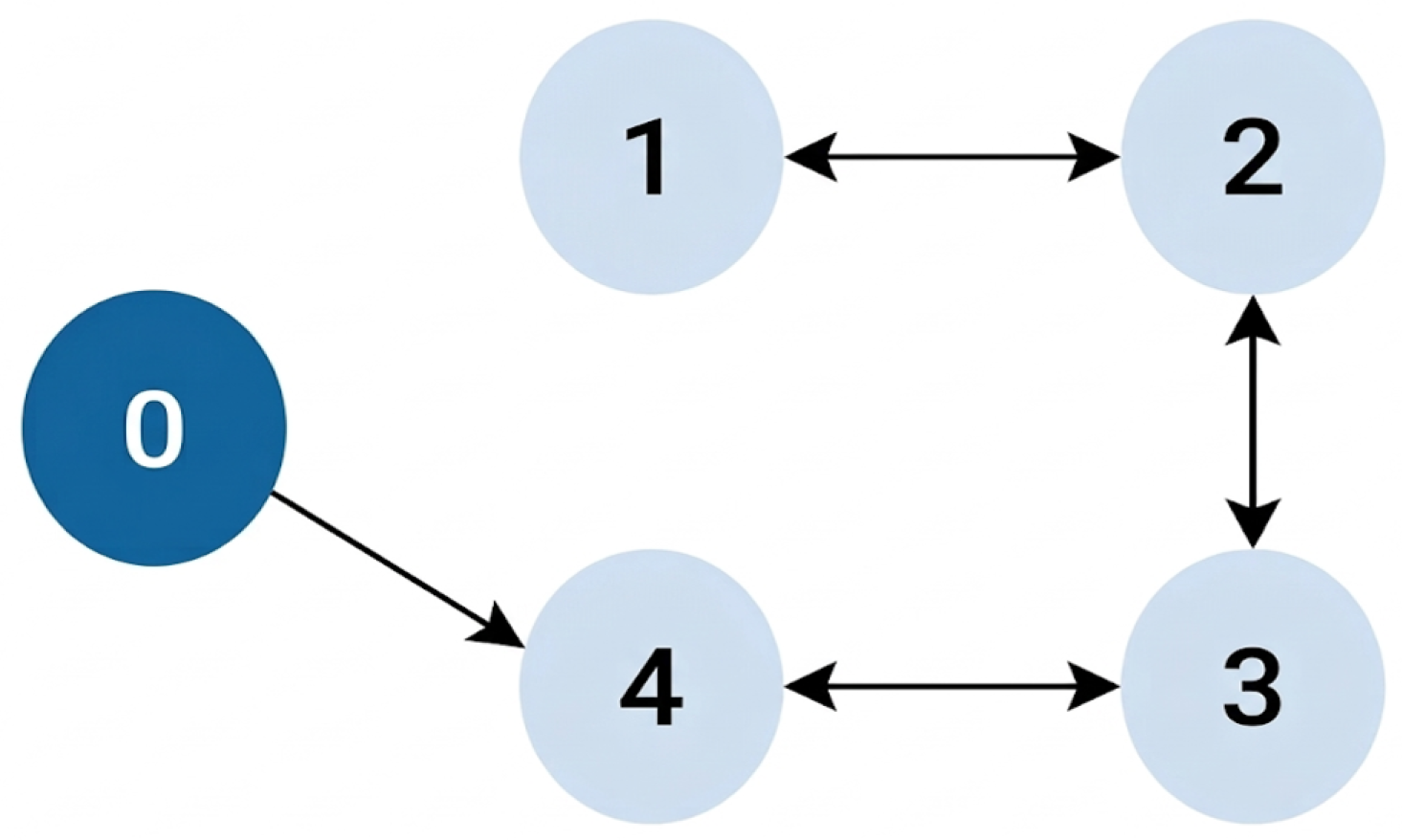
The communication topology of the follower spacecraft in TSNR system is described bythe directed graph $\mathcal{G}$. As illustrated in Figure 2, each follower exchanges information with its neighbors to achieve coordinated behavior. The adjacency matrix ${\mathit{A}}_{\mathcal{G}}\in {\mathbb{R}}^{5\times 5}$ is determined as follows:

$${\mathit{A}}_{\mathcal{G}}=\left[\begin{array}{ccccc}0& 0& 0& 0& 0\\ 0& 0& 1& 0& 0\\ 0& 1& 0& 1& 0\\ 0& 0& 1& 0& 1\\ 1& 0& 0& 1& 0\end{array}\right].$$

The follower spacecraft start with the following initial states: ${\mathit{x}}_1\left(0\right)={[0,-6,5,0,0,0]}^{\top }$, ${\mathit{x}}_2\left(0\right)={[0,-5,-5.5,0,0,0]}^{\top }$, ${\mathit{x}}_3\left(0\right)={[0,6,-5,0,0,0]}^{\top }$, and ${\mathit{x}}_4\left(0\right)={[0.5,5,5,0,0,0]}^{\top }$. The desired relative formation vectors are defined as ${\mathit{d}}_{12}={[0,0,12]}^{\top }$, ${\mathit{d}}_{23}={[0,-12,0]}^{\top }$, and ${\mathit{d}}_{34}={[0,-12,0]}^{\top }$.System and control parameters are summarized as follows:

• Orbital Dynamics: The mean motion is ${\omega }_0=7.2388\times {10}^{-5}{\mathrm{s}}^{-1}$.
• Safety Constraints: To ensure net integrity and collision avoidance, the inter-spacecraft distance bounds are set to $\underline{R}=10\mathrm{m}$ and $\overline{R}=15\mathrm{m}$.
• MPC Settings: The prediction horizon $N=6$, and the total simulation duration $T=100\mathrm{s}$. The sampling period $\Delta t=0.1\mathrm{s}$. Control inputs are subject to an upper bound of $u_{max}=0.02{\mathrm{m}/\mathrm{s}}^2$.
• Weighting Matrices: The cost function weights are chosen as ${\mathit{Q}}_i=5{\mathit{I}}_6$, ${\mathit{Q}}_{\mathit{\chi }}={\mathit{I}}_6$, ${\mathit{Q}}_{\mathit{e}}={\mathit{I}}_6$, and ${\mathit{R}}_i={\mathit{I}}_3$.
• Auxiliary Control: The auxiliary control parameters are selected as ${\mathit{A}}_{\psi }=0.5{\mathit{I}}_6,{\mathit{B}}_{\psi }=0.1{\mathit{I}}_6,{\mathit{C}}_{\psi }=-0.75{\mathit{I}}_6$, and ${\mathit{D}}_{\psi }=-\mathit{A}$. Under this selection, the augmented system matrix ${\mathit{A}}_{\mathit{\chi }}$ satisfies the Schur stability condition. In practice, this can be achieved via pole placement, where the eigenvalues of ${\mathit{A}}_{\mathit{\chi }}$ are assigned inside the unit circle. The gain matrix ${\mathit{K}}_{{\widehat{\mathit{u}}}_i}$ is designed as:

  $${\mathit{K}}_{{\widehat{\mathit{u}}}_i}=\left[\begin{array}{cccccc}9.4& 0.0& 0.0& 10.4& 0.0& 0.0\\ 0.0& 9.4& 0.0& 0.0& 10.4& 0.0\\ 0.0& 0.0& 9.4& 0.0& 0.0& 10.4\end{array}\right]$$

  (23)
  This configuration guarantees the stability of the closed-loop error matrix ${\mathit{A}}_{\mathit{e}}$, with all eigenvalues strictly located inside the unit circle, as established in Theorem 1.

To ensure reproducibility, the proposed TSNR formation control scheme is implemented in MATLAB 2024b, with the DLMPC optimization subproblems solved using the fmincon solver based on the Sequential Quadratic Programming (SQP) algorithm. Simulations were conducted on a workstation equipped with a 3.0 GHz processor and 64 GB of RAM. The results yield an average execution time of 0.064 s per control step. Given that a compiled C++ implementation typically offers a significant speedup over interpreted MATLAB code on embedded platforms, these results underscore the algorithm’s potential for real-time deployment on satellite flight computers.

4.1.2. Reference Trajectory and Disturbances

The nominal reference trajectory for the TSNR geometric center is given by:

$$r_x\left(t\right)=0.004t^2,r_y\left(t\right)=4cos\left(0.04t\right),r_z\left(t\right)=3.5sin\left(0.05t\right).$$

The reference acceleration is constrained within $0.01{\mathrm{m}/\mathrm{s}}^2$.

To examine the resilience of the DLMPC framework, three distinct disturbance scenarios are considered as follows:

• Random Disturbance ${\mathit{f}}_1$: Uniformly distributed noise within the range $(-0.005,0.005){\mathrm{m}/\mathrm{s}}^2$ for each axis.
• Time-Varying Disturbance ${\mathit{f}}_2$: For each spacecraft $i\in \{1,\dots ,4\}$, the external disturbance acceleration along each axis is modeled as a composite sinusoidal signal:

  $$\left\{\begin{array}{c}{f}_{i,x}\left(t\right)=0.006sin(0.5t+{\displaystyle \frac{i\pi }{3}})+0.002cos\left(1.2t\right),\hfill \\ f_{i,y}\left(t\right)=0.005sin(0.8t+{\displaystyle \frac{i\pi }{3}})+0.003sin\left(2t\right),\hfill \\ f_{i,z}\left(t\right)=0.007cos(0.4t+{\displaystyle \frac{i\pi }{3}})+0.001sin\left(1.5t\right).\hfill \end{array}\right.$$

  (24)
• State-Dependent Disturbance ${\mathit{f}}_3$: The disturbance incorporates nonlinear coupling of the velocity states and time-varying components to simulate the disturbance:

  $$\left\{\begin{array}{c}{f}_{i,x}(\dot{\mathit{x}},t)={\dot{x}}_i{\dot{y}}_i+0.005sin(t+{\displaystyle \frac{i\pi }{3}}),\hfill \\ f_{i,y}(\dot{\mathit{x}},t)={\dot{x}}_i{\dot{y}}_i{\dot{z}}_i+0.004cos(0.5t+{\displaystyle \frac{i\pi }{3}})+0.005,\hfill \\ f_{i,z}(\dot{\mathit{x}},t)=({\dot{x}}_i+{\dot{y}}_i{\dot{z}}_i)+0.006sin(0.8t+{\displaystyle \frac{i\pi }{3}}),\hfill \end{array}\right.$$

  (25)

  where each component is saturated at $\pm 0.01{\mathrm{m}/\mathrm{s}}^2$ to represent the physical bounds of the disturbance.

4.1.3. Dynamics of the Tethered Net

While a full physical model capturing tether elasticity and wave propagation offers higher fidelity, its integration into the predictive horizon would impose a prohibitive computational burden for real-time control. To resolve this, our controller treats the net dynamics as a constituent of the bounded disturbances addressed in this study, utilizing an observer-embedded framework to estimate and compensate for the model mismatch in real-time. Crucially, to rigorously validate the controller’s performance, a high-fidelity lumped mass model is employed during the simulation phase to represent the physical tethered net. This setup ensures that the controller is tested against realistic nonlinear behaviors that were intentionally omitted during the design phase to maintain computational efficiency. However, it should be noted that as a trade-off for this efficiency, the controller cannot explicitly regulate the net’s oscillations during capture, since these complex internal dynamics are not directly incorporated into the control law.

In this simulation environment, the tethered net is discretized into a $9\times 9$ grid of nodes. The mass $m_i$ concentrated at each node i is calculated by summing half of the masses of the adjacent cable elements connected to it, expressed as:

$$m_i=\left\{\begin{array}{cc}2\rho A{l}_0,\hfill & i\mathrm{is}\mathrm{inside}\mathrm{the}\mathrm{net},\hfill \\ 3/2\rho A{l}_0,\hfill & i\mathrm{is}\mathrm{on}\mathrm{the}\mathrm{four}\mathrm{edges},\hfill \\ \rho A{l}_0,\hfill & i\mathrm{is}\mathrm{at}\mathrm{the}\mathrm{four}\mathrm{corner}/\mathrm{towing}\mathrm{points},\hfill \end{array}\right.$$

where $\rho$ is the cable density, A is the cross-sectional area, and $l_0$ is the unstretched length of each element. Furthermore, to capture the inherent physical properties of the flexible net—specifically that cables provide no resistance to compression—we utilized the Kelvin–Voigt model. The tension force vector ${\mathit{T}}_{i,j}$ between nodes i and j is defined as:

$${\mathit{T}}_{i,j}=\left\{\begin{array}{cc}\left[-k_{ij}(l_{ij}-l_0)-c_{ij}({\mathit{v}}_{ij}·{\mathit{r}}_{ij})\right]{\mathit{r}}_{ij},\hfill & \mathrm{if}{l}_{ij}>l_0,\hfill \\ 0,\hfill & \mathrm{if}{l}_{ij}\le l_0,\hfill \end{array}\right.$$

where ${\mathit{r}}_{ij}$ and ${\mathit{v}}_{ij}$ represent the relative position and velocity vectors between consecutive masses. The axial stiffness is defined as $k_{ij}=EA/l_0$ (where E is Young’s modulus), and the damping coefficient is $c_{ij}=2\xi \sqrt{m_{ij}{k}_{ij}}$, with $\xi$ denoting the damping ratio. The specific values for the parameters mentioned above are summarized in

Table 1. Simulation parameters of the tethered net.

Parameters	Value
Side Length $L_{net}$	8 m
Length of towing cable $L_t$	3 m
Mesh Length $l_0$	1 m
Tether Density $\rho$	1440 $\mathrm{kg}/{\mathrm{m}}^3$
Tether Young’s Modulus E,	124 GPa
Tether Radius r	0.005 m
Tether Damping Ratio $\xi$	0.1

.

4.2. Results and Discussion

4.2.1. Formation Tracking and Net Configuration

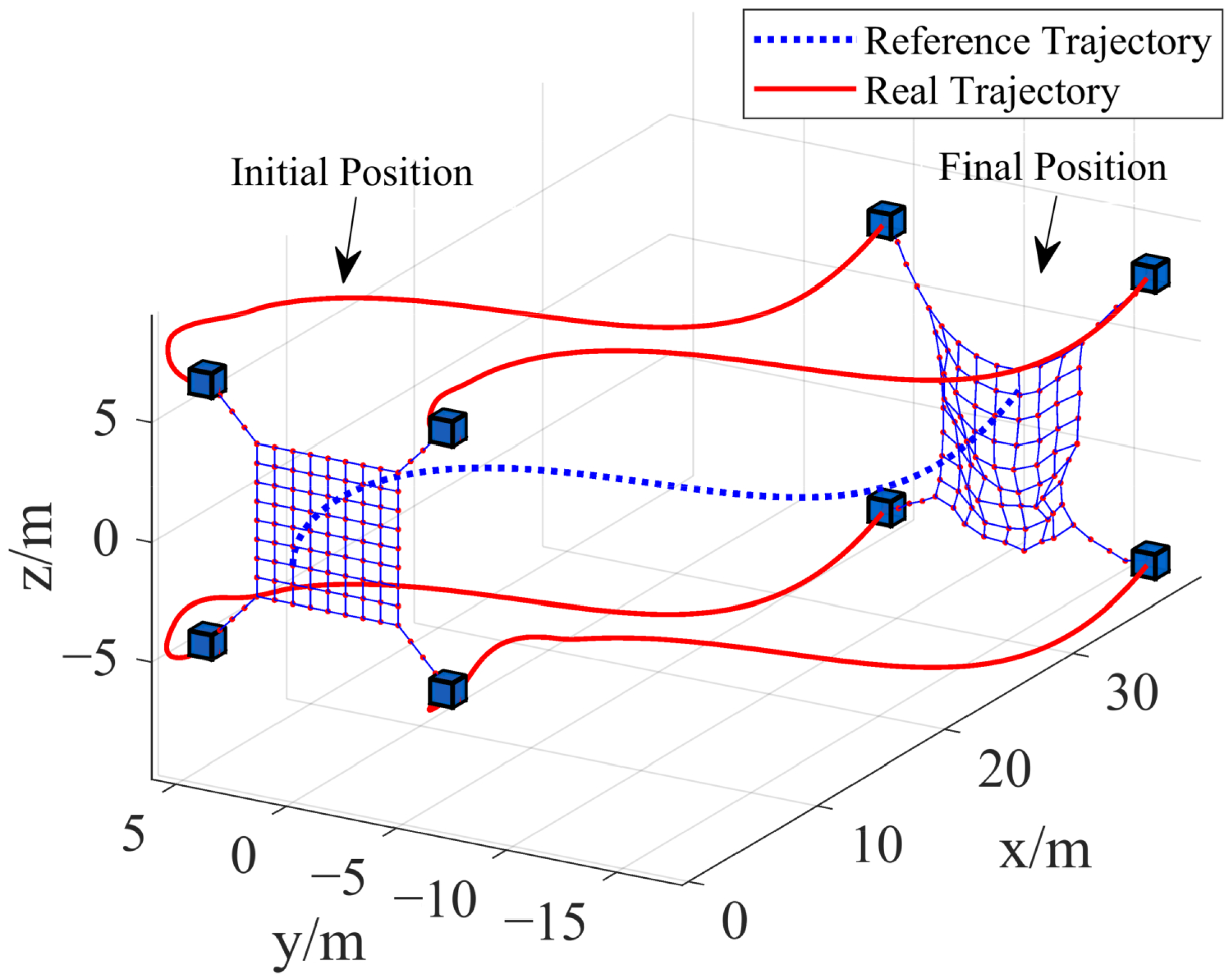
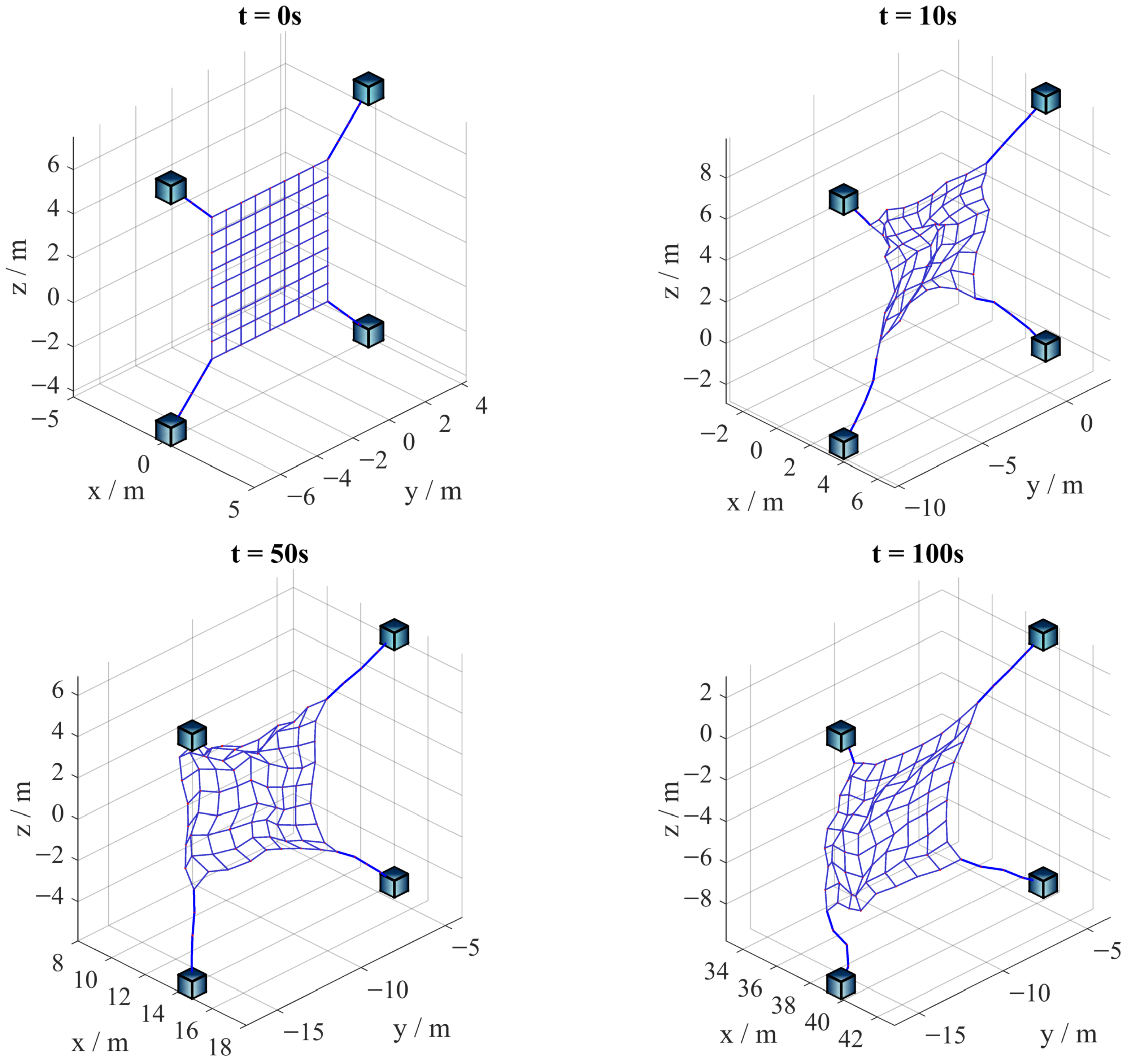
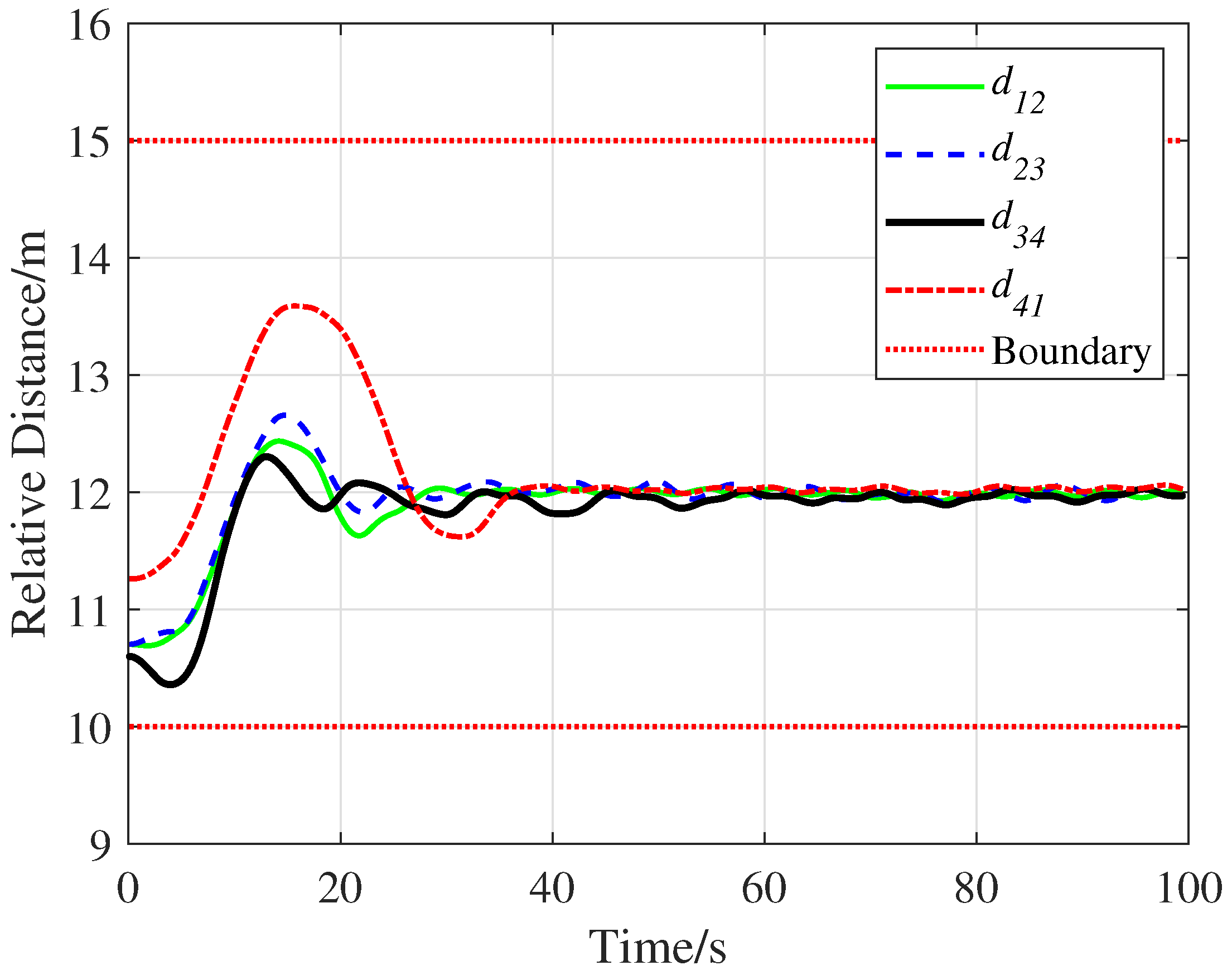
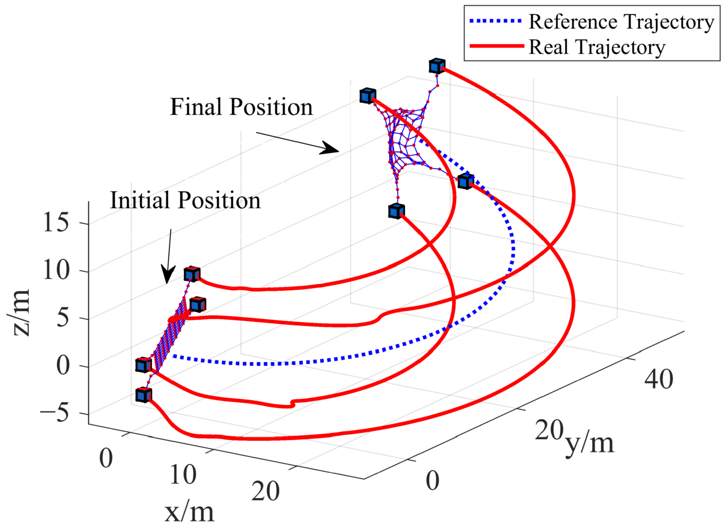
Simulations are first carried out under the specified settings and the assumed unknown disturbance ${\mathit{f}}_3$ to evaluate the proposed DLMPC algorithm. The resulting three-dimensional trajectories, illustrated in Figure 3, show that all follower spacecraft converge to the desired path while preserving the prescribed formation geometry. Figure 4 illustrates the dynamic evolution of the tethered net configuration. Notably, the inter-spacecraft distances are strictly maintained within the safety bounds, ensuring that the tethered net remains effectively deployed without incurring slack or excessive tension.

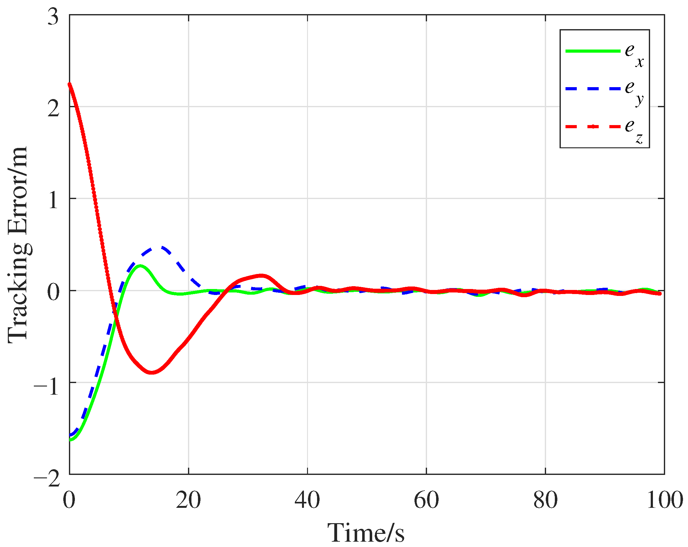
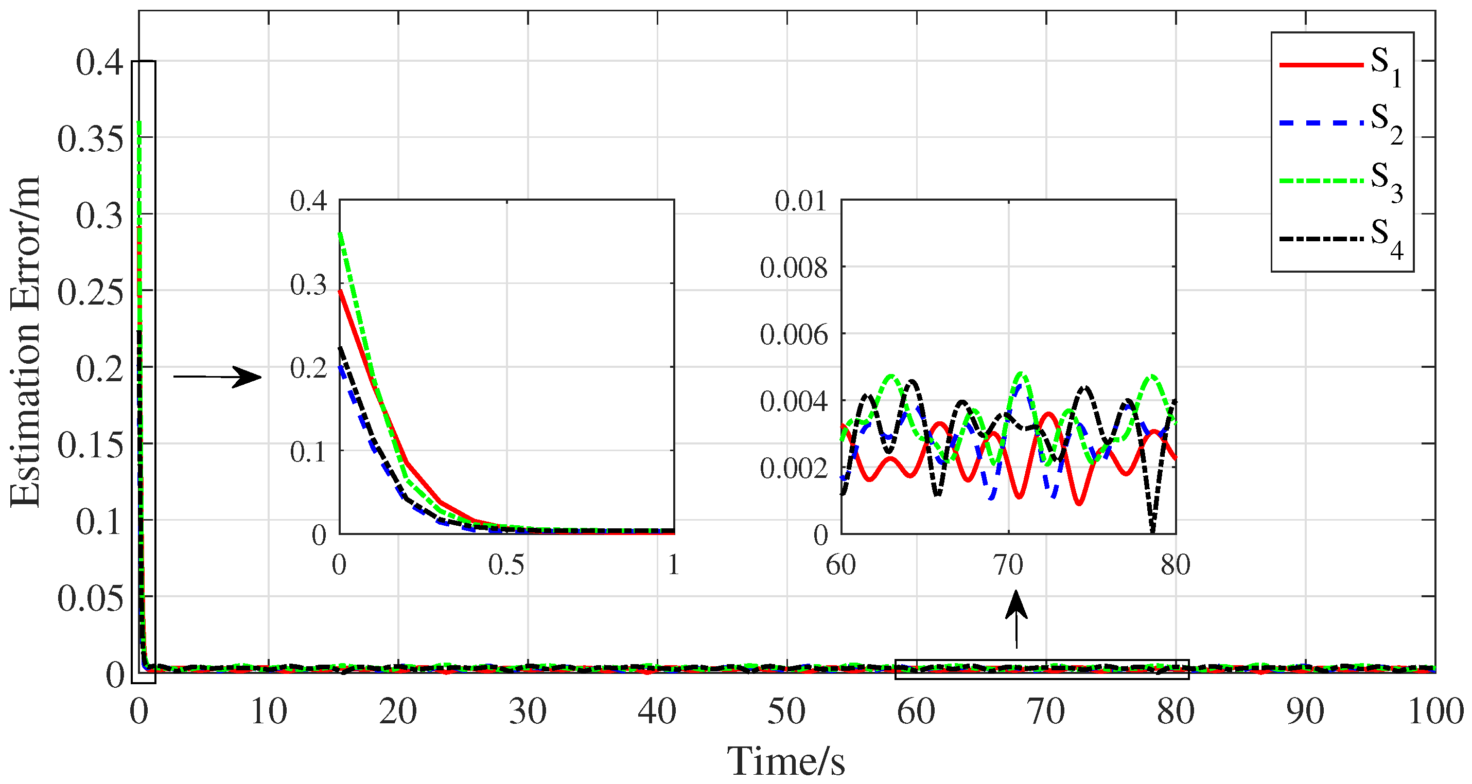
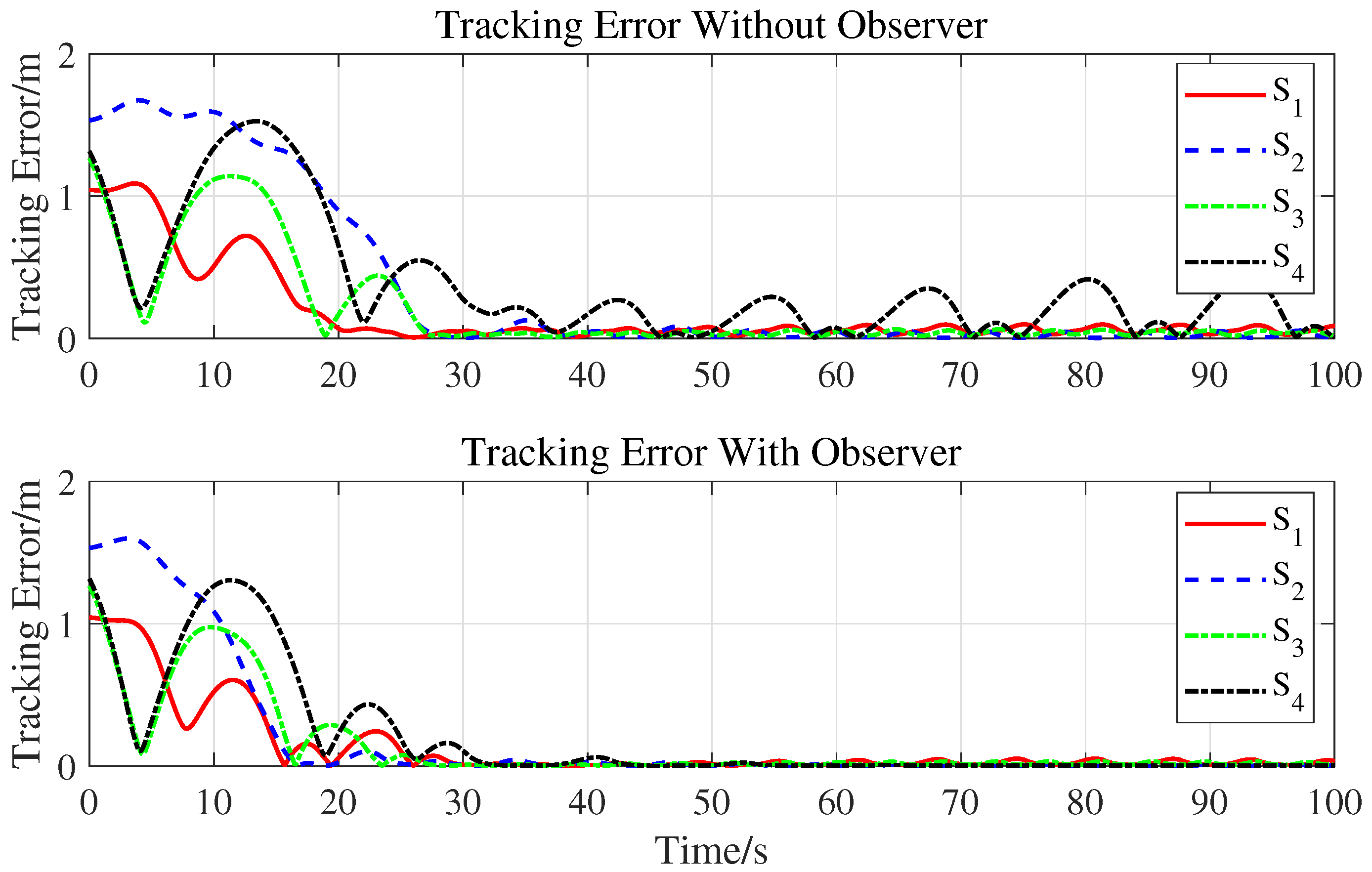
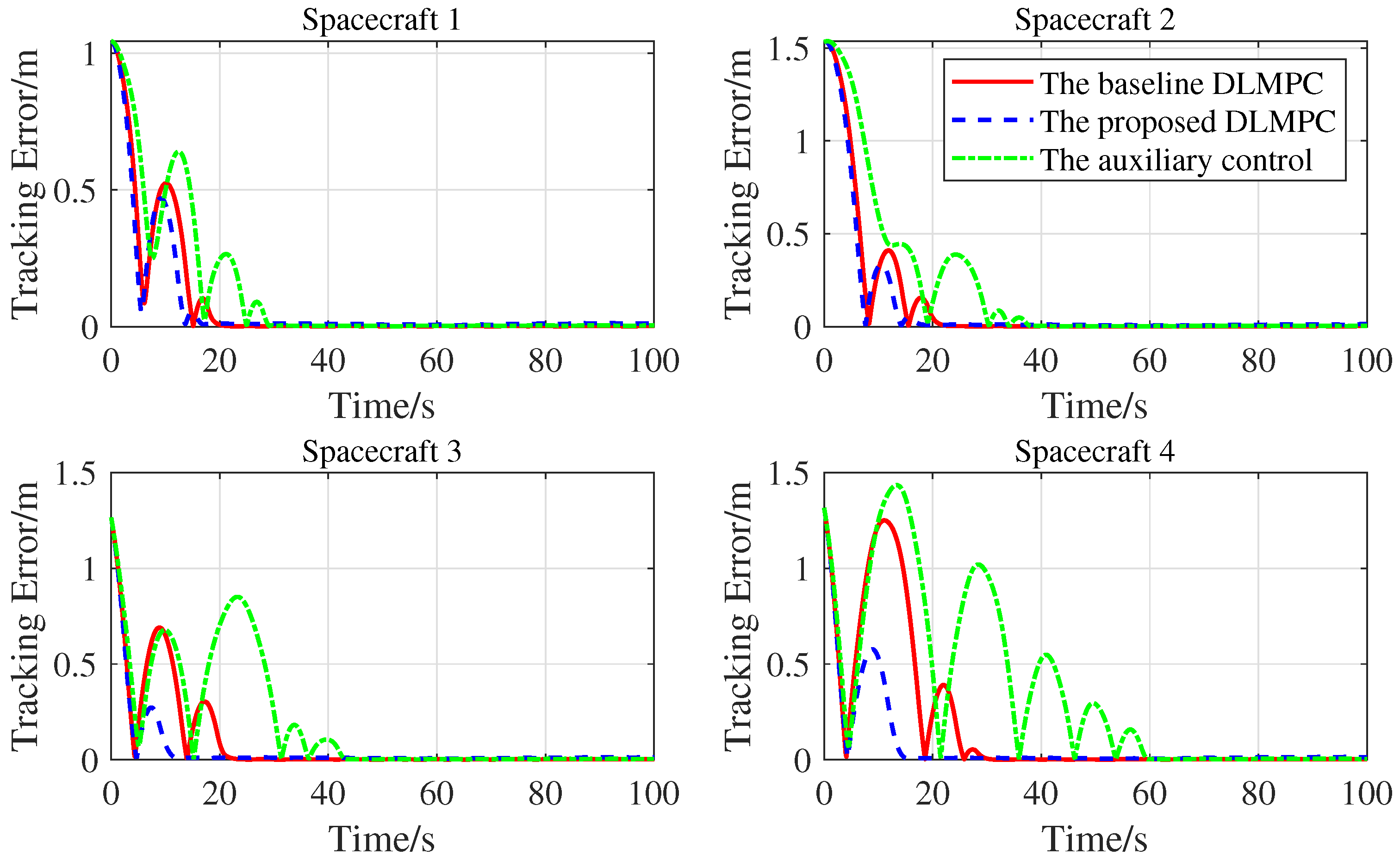
Figure 5 and Figure 6 depict the tracking errors of the formation center and configuration, respectively. The errors exhibit smooth convergence toward a small neighborhood around zero, validating the effectiveness of the proposed DLMPC in coordinating multi-agent maneuvers under the unknown bounded disturbanc. It is clearly seen from Figure 7 that the estimation error converges rapidly based on the observer, allowing the DLMPC to explicitly compensate for the disturbances in the prediction model. As a result, as illustrated in Figure 8, the tracking error for each spacecraft $S_i$ converges more rapidly and maintains a smaller value at steady state.

4.2.2. Robustness and Comparative Analysis

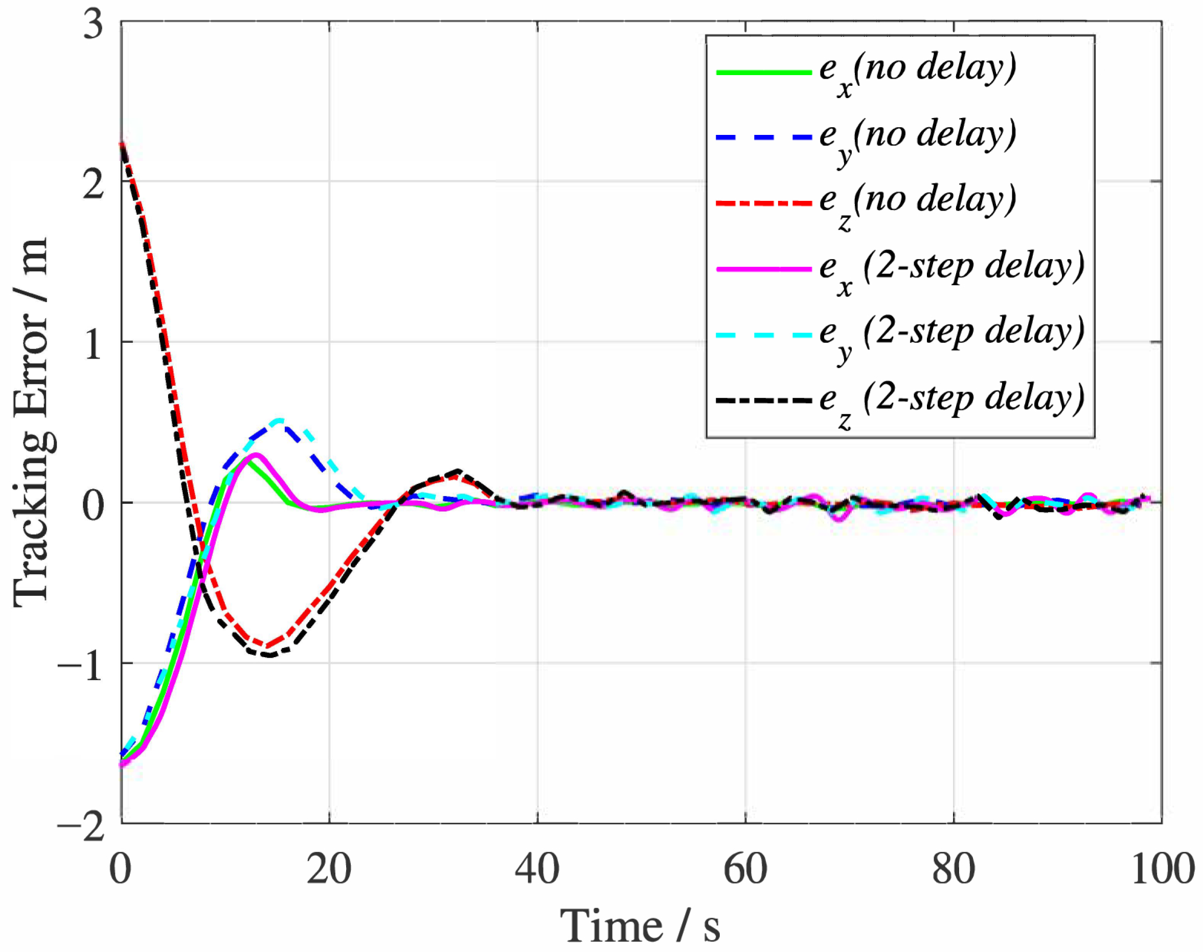
To evaluate the robustness of the proposed method against communication delays, a two-step delay is introduced in the information exchange among agents. Specifically, the information received from neighboring spacecraft is modified from ${\mathit{x}}_j^a(k+n\mid k)$ to ${\mathit{x}}_j^a(k+n\mid k-2)$. Figure 9 shows that the tracking performance is only slightly degraded, which demonstrates the robustness of the proposed approach to short-term communication delays.

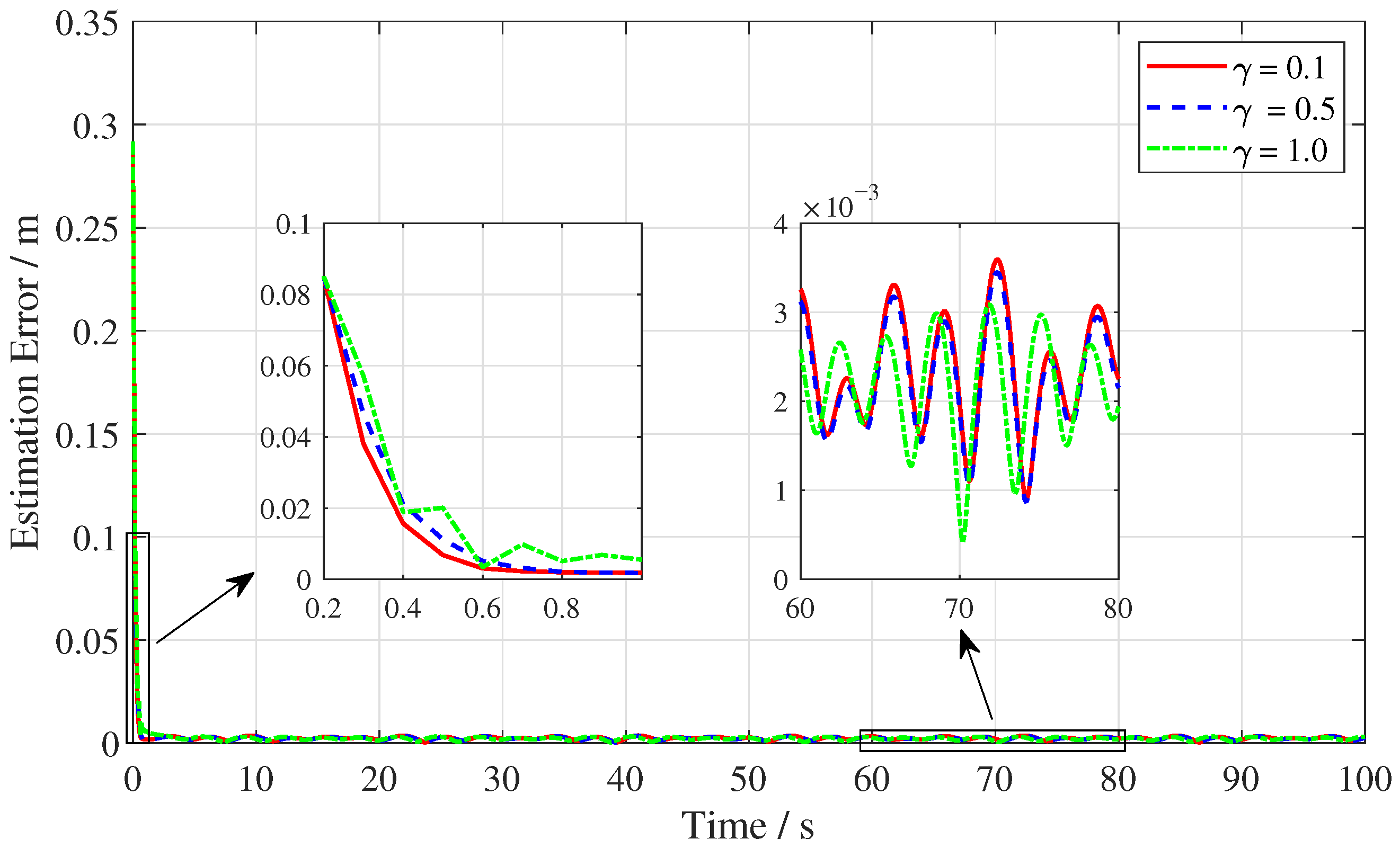
To evaluate the sensitivity of the observer design, the parameter ${\mathit{A}}_{\psi }$ is varied as ${\mathit{A}}_{\psi }=\gamma \mathit{I}$ with $\gamma \in \{0.1,0.5,1\}$. For all selected values, the resulting augmented system matrix ${\mathit{A}}_{\chi }$ has eigenvalues strictly inside the unit circle, ensuring Schur stability. As shown in Figure 10, smaller values of $\gamma$ lead to faster convergence of the estimation error, but introduce more pronounced oscillations due to noise amplification. In contrast, larger values of $\gamma$ result in smoother responses with slightly slower convergence. Overall, the differences in estimation performance remain moderate across the tested range, indicating that the proposed observer is not overly sensitive to parameter variations, provided that the stability condition is satisfied.

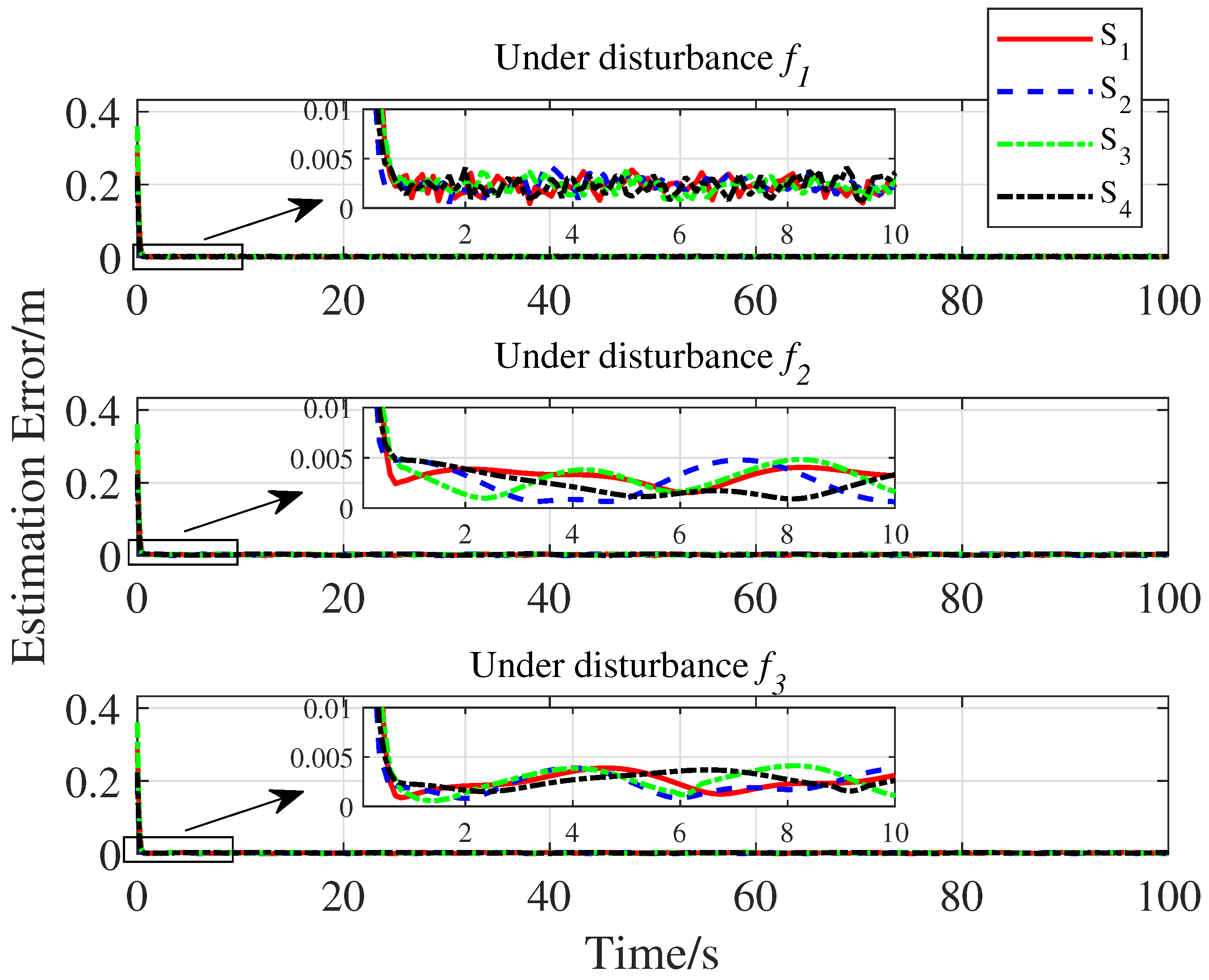
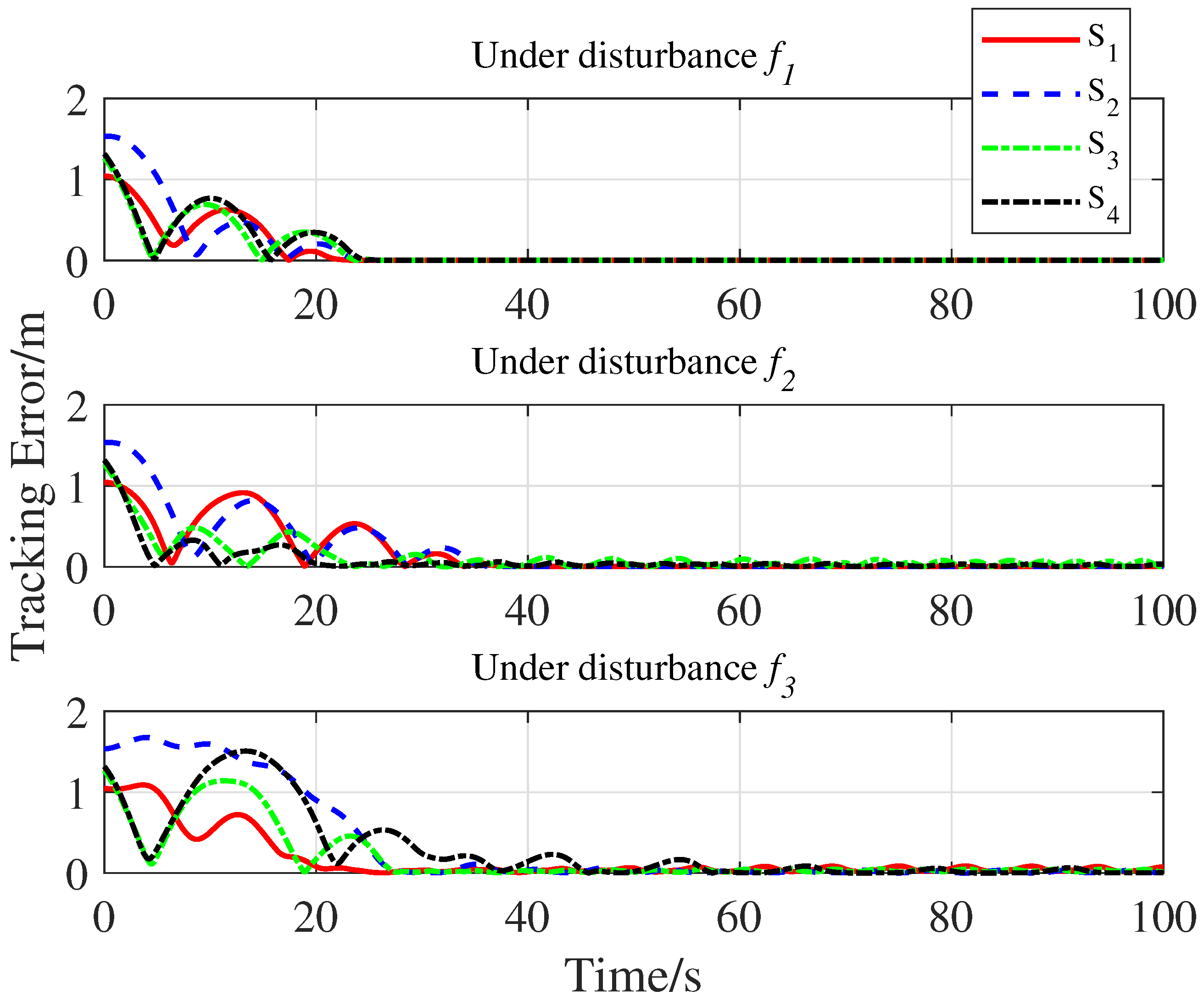
Under random, time-varying, and state-dependent disturbance profiles, both estimation and tracking errors remain bounded and converge to minimal steady-state values as shown in Figure 11 and Figure 12. This confirms that the DLMPC approach can maintain high tracking precision across diverse disturbances. Finally, a performance comparison is presented in Figure 13. The proposed DLMPC significantly outperforms the auxiliary control and standard DLMPC baselines. These results highlight the superiority of integrating a disturbance observer with a Lyapunov-based contraction constraint for TSNR formation control.

To assess the versatility and robustness of the proposed DLMPC algorithm, an alternative set of time-varying reference trajectories for the TSNR geometric center is considered over a simulation duration of $T=150$ s:

$$r_x\left(t\right)=20sin\left({\displaystyle \frac{\pi }{150}}t\right),r_y\left(t\right)=20-20cos\left({\displaystyle \frac{\pi }{150}}t\right),r_z\left(t\right)=0.0005t^2.$$

The three-dimensional tracking performance under this complex maneuvering scenario is illustrated in Figure 14. It is clearly shown that the proposed method consistently achieves high-precision formation tracking, with the TSNR system effectively following the curved reference path while maintaining the internal configuration constraints. The results demonstrate that the DLMPC framework is also generalizes well to diverse mission scenarios, ensuring reliable convergence and stability throughout the entire flight envelope.

5. Conclusions

This paper proposed an observer-embedded distributed Lyapunov-based model predictive control framework for disturbance-resilient formation tracking of tethered space net robots. By explicitly incorporating disturbance estimation into the prediction model, the proposed approach effectively reduces the mismatch between predicted and actual system dynamics, thereby improving tracking accuracy under complex unknown bounded disturbances. A worst-case contraction constraint was further developed to guarantee recursive feasibility and robust closed-loop stability in the presence of unknown bounded disturbance. Theoretical analysis established the uniform ultimate boundedness of the closed-loop system, while ensuring that safety constraints are rigorously satisfied. Simulation results demonstrated that the proposed method significantly outperforms both conventional auxiliary control and standard DLMPC approaches in terms of tracking precision, robustness, and constraint satisfaction.

Despite these promising results, several challenges remain. In this study, the target is assumed to follow a known or predictable reference trajectory, and disturbances are modeled as bounded uncertainties. However, in practical space missions, debris objects are typically uncooperative, maneuver unpredictably, and are only partially observable. Furthermore, the simplified tether model used in this validation may not fully capture the complex nonlinear dynamics in real orbital scenarios. These characteristics introduce significant challenges in perception, decision-making, and control. Future work will focus on extending the proposed framework to address the cooperative capture of non-cooperative space debris under incomplete information, incorporating higher-fidelity physical models.

References

1. Liu, C.; Luo, Y.; Yue, X.; Li, S. Hierarchical cooperative adaptive model predictive control for swarm self-assembly of large-scale spacecraft. Aerosp. Sci. Technol. 2025, 170, 111538. [Google Scholar] [CrossRef] [Scilit]
2. Wei, C.; Huang, G.; Wang, Z.; Dai, H.; Wang, Y. Distributed Analytic Predictive Control for Multi-Spacecraft Cooperatively Flying Around a Non-Cooperative Target. IEEE Trans. Aerosp. Electron. Syst. 2025, 61, 10024–10037. [Google Scholar] [CrossRef] [Scilit]
3. Zhu, W.; Pang, Z.; Du, Z.; Gao, G.; Zhu, Z.H. Multi-debris capture by tethered space net robot via redeployment and assembly. J. Guid. Control Dyn. 2024, 47, 1359–1376. [Google Scholar] [CrossRef] [Scilit]
4. Hong, A.A.T.; Varatharajoo, R.; Chak, Y.C. Review of deployment controllers for space tethered system. Adv. Space Res. 2025, 75, 3933–3949. [Google Scholar] [CrossRef] [Scilit]
5. Wang, C.; Zhang, F. Strict finite-time sliding mode control for a tethered space net robot. Chin. J. Aeronaut. 2023, 36, 325–335. [Google Scholar] [CrossRef] [Scilit]
6. Ma, Y.; Zhang, Y.; Liu, Y.; Huang, P.; Zhang, F. An active energy management distributed formation control for tethered space net robot via cooperative game theory. Acta Astronaut. 2025, 227, 57–66. [Google Scholar] [CrossRef] [Scilit]
7. Aglietti, G.S.; Taylor, B.; Fellowes, S.; Ainley, S.; Tye, D.; Cox, C.; Zarkesh, A.; Mafficini, A.; Vinkoff, N.; Bashford, K.; et al. RemoveDEBRIS: An in-orbit demonstration of technologies for the removal of space debris. Aeronaut. J. 2020, 124, 1–23. [Google Scholar] [CrossRef] [Scilit]
8. Liu, Y.; Ma, Z.; Zhang, F.; Huang, P. Time-varying formation planning and scaling control for tethered space net robot. IEEE Trans. Aerosp. Electron. Syst. 2023, 59, 6717–6728. [Google Scholar] [CrossRef] [Scilit]
9. Liu, F.; Boonrath, A.; Botta, E.M.; Chowdhury, S. Surrogate-aided Learning of Active Tether-Net Maneuver to Capture Rotating Space Debris. IEEE Trans. Aerosp. Electron. Syst. 2025, 62, 630–645. [Google Scholar] [CrossRef] [Scilit]
10. Ma, Y.; Zhang, Y.; Huang, P.; Liu, Y.; Zhang, F. Game theory based finite-time formation control using artificial potentials for tethered space net robot. Chin. J. Aeronaut. 2024, 37, 358–372. [Google Scholar] [CrossRef] [Scilit]
11. O’Connor, M.; Simoneau, A.; Dubay, R. Model Predictive Control of Underwater Tethered Payload. Appl. Sci. 2025, 15, 10122. [Google Scholar] [CrossRef] [Scilit]
12. Reiter, R.; Hoffmann, J.; Reinhardt, D.; Messerer, F.; Baumgärtner, K.; Sawant, S.; Boedecker, J.; Diehl, M.; Gros, S. Synthesis of model predictive control and reinforcement learning: Survey and classification. Annu. Rev. Control 2026, 61, 101045. [Google Scholar] [CrossRef] [Scilit]
13. Wang, M.; Zhao, C.; Xia, J.; Sun, J. Periodic event-triggered robust distributed model predictive control for multiagent systems with input and communication delays. IEEE Trans. Ind. Inf. 2023, 19, 11216–11228. [Google Scholar] [CrossRef] [Scilit]
14. Liu, A.; Zhang, W.A.; Yu, L.; Yan, H.; Zhang, R. Formation control of multiple mobile robots incorporating an extended state observer and distributed model predictive approach. IEEE Trans. Syst. Man Cybern. Syst. 2018, 50, 4587–4597. [Google Scholar] [CrossRef] [Scilit]
15. Yuan, Q.; Li, X. Distributed model predictive formation control for a group of UAVs with spatial kinematics and unidirectional data transmissions. IEEE Trans. Netw. Sci. Eng. 2023, 10, 3209–3222. [Google Scholar] [CrossRef] [Scilit]
16. Liu, Y.; Wu, Y.; Zhang, F.; Huang, P.; Lu, Y.; Chang, H. Collision-free Trajectory Generation and Robust Nonlinear Distributed Model Predictive Control for Tethered Multi-rotor Unmanned Aerial Vehicles. IEEE Trans. Autom. Sci. Eng. 2026, 23, 4819–4832. [Google Scholar] [CrossRef] [Scilit]
17. Du, Z.; Zhang, H.; Wang, Z.; Yan, H. Model predictive formation tracking-containment control for multi-UAVs with obstacle avoidance. IEEE Trans. Syst. Man Cybern. Syst. 2024, 54, 3404–3414. [Google Scholar] [CrossRef] [Scilit]
18. Xu, B.; Dai, Y.; Suleman, A.; Shi, Y. Distributed fault-tolerant control of multi-UAV formation for dynamic leader tracking: A Lyapunov-based MPC framework. Automatica 2025, 175, 112179. [Google Scholar] [CrossRef] [Scilit]
19. Hao, L.Y.; Zhou, Y.; Wang, R.Z.; Zhao, X. Finite-Time Lyapunov-Based Model Predictive Control of ASVs: An Enlarging Attraction Domain Strategy Against DoS Attacks. IEEE Trans. Intell. Transp. Syst. 2025, 26, 23257–23268. [Google Scholar] [CrossRef] [Scilit]
20. Nie, Y.; Yuan, Q.; Li, X. A tracking control approach with sequence-scaling Lyapunov-based MPC for quadruped robots. IEEE Trans. Ind. Inf. 2024, 20, 10728–10737. [Google Scholar] [CrossRef] [Scilit]
21. Cui, Y.; Chen, Y.; Yang, D.; Shu, Z.; Huang, T.; Gong, X. Resilient formation tracking of spacecraft swarm against actuation attacks: A distributed Lyapunov-based model predictive approach. IEEE Trans. Syst. Man Cybern. Syst. 2023, 53, 7053–7065. [Google Scholar] [CrossRef] [Scilit]
22. Nie, Y.; Li, X. Antidisturbance distributed lyapunov-based model predictive control for quadruped robot formation tracking. IRE Trans. Ind. Electron. 2025, 72, 10359–10369. [Google Scholar] [CrossRef] [Scilit]
23. Wei, H.; Shen, C.; Shi, Y. Distributed Lyapunov-based model predictive formation tracking control for autonomous underwater vehicles subject to disturbances. IEEE Trans. Syst. Man Cybern. Syst. 2019, 51, 5198–5208. [Google Scholar] [CrossRef] [Scilit]
24. Jia, Z.; Zhang, K.; Shi, Y.; Zhang, W. Safety-preserving Lyapunov-based model predictive rendezvous control for heterogeneous marine vehicles subject to external disturbances. IEEE Trans. Cybern. 2024, 54, 5244–5256. [Google Scholar] [CrossRef] [Scilit] [PubMed]
25. Long, C.; Hu, M.; Bian, Y.; Chang, D. SREDFTC: A Safe, Robust and Efficient Distributed Formation Tracking Controller for Nonlinear Multi-UUV Systems. Nonlinear Dyn. 2025, 113, 21601–21629. [Google Scholar] [CrossRef] [Scilit]
Figure 1. Schematic of the TSNR formation tracking.
Applsci 16 04344 g001
Figure 2. The communication topology graph of the TSNR system. Node 0 represents the virtual leader, and nodes 1–4 denote the spacecraft in the formation. An arrow pointing from i to j indicates that j can receive information from i.
Applsci 16 04344 g002
Figure 3. An illustration of three-dimensional formation tracking trajectories of the TSNR system under the proposed DLMPC framework.
Applsci 16 04344 g003
Figure 4. Snapshots of the tethered net configuration at different time.
Applsci 16 04344 g004
Figure 5. The tracking errors of the TSNR’s geometric center.
Applsci 16 04344 g005
Figure 6. Relative formation tracking errors of the neighboring spacecraft.
Applsci 16 04344 g006
Figure 7. The estimation errors by adopting the observer for each spacecraft S i .
Applsci 16 04344 g007
Figure 8. Comparison of tracking errors with or without an observer.
Applsci 16 04344 g008
Figure 9. The tracking errors of the TSNR’s geometric center under communication delays.
Applsci 16 04344 g009
Figure 10. Sensitivity analysis of the observer with respect to the parameter γ .
Applsci 16 04344 g010
Figure 11. Comparison of observer estimation errors under random, time-varying, and state-dependent disturbance scenarios.
Applsci 16 04344 g011
Figure 12. Comparison of formation tracking errors under different disturbance scenarios.
Applsci 16 04344 g012
Figure 13. Comparative analysis of tracking errors between the proposed DLMPC, standard DMPC, and auxiliary control.
Applsci 16 04344 g013
Figure 14. Three-dimensional formation tracking trajectories of the TSNR system.
Applsci 16 04344 g014