Article

Adaptive Data-Driven Control of Autonomous Underwater Vehicles: Bridging the Gap Between Simulation and Experimental Baseline via LSTM-MPC

by
Ahmetcan Önal
1,2,* and
Andaç Töre Şamiloğlu
2
1
Roketsan Inc., Ankara 06780, Turkey
2
Mechanical Engineering Department, Başkent University, Ankara 06790, Turkey
*
Author to whom correspondence should be addressed.
Appl. Sci. 2026, 16(9), 4187; https://doi.org/10.3390/app16094187
Submission received: 26 January 2026 / Revised: 25 February 2026 / Accepted: 26 February 2026 / Published: 24 April 2026
(This article belongs to the Special Issue Data-Driven Control System: Methods and Applications)

Featured Application

The proposed LSTM–MPC framework is particularly suited for autonomous inspection of offshore structures, coastal monitoring tasks and experimental AUV operations where environmental variability and plant–model mismatch cannot be neglected.

Abstract

This study proposes a robust data-driven control framework, LSTM-MPC, designed to enhance the velocity stabilization of Autonomous Underwater Vehicles (AUVs) operating under stochastic marine disturbances. Traditional control methods often struggle with the highly nonlinear and time-varying hydrodynamics of irregular waves. To address this, we employ a Long Short-Term Memory (LSTM) recurrent neural network to capture complex temporal dependencies and provide accurate multi-step-ahead velocity predictions. These predictions are integrated into a Model Predictive Control (MPC) scheme, which optimizes control actions while respecting actuator constraints. A key contribution is the integration of an error-triggered online learning mechanism. Utilizing run-time weight synchronization via MATLAB Coder, the framework dynamically adapts to plant mismatches and high-frequency MEMS noise without an explicit analytical model. The architecture was validated using experimental data from a Pixhawk/ArduSub baseline. Results demonstrate that, under these stochastic conditions, the data-driven approach significantly outperforms the standard PID-based baseline. While adaptive PID variants offer improvements, the suggested framework drastically reduces tracking errors in rotational axes while maintaining high precision in translational velocities. This research confirms that adaptive, data-driven strategies can effectively bridge the gap between simulation and real-world deployment, offering a scalable solution for robust AUV autonomy in unpredictable environments.

1. Introduction

Unmanned Underwater Vehicles (UUVs) have gained increasing importance in recent years in defense industry, marine science and industrial inspection applications. The concept of UUVs is originally based on tethered remotely operated underwater vehicles (ROVs) that were used in oil and natural gas exploration activities in the 1960s. In these systems, the physical cable between the carrier platform and the vehicle provides a power supply and bidirectional data transmission. Although the tethered architecture is advantageous in terms of high bandwidth and operator intervention, it introduces operational limitations due to restricted maneuverability and additional dynamic effects caused by cable drag.
Recent research has shifted toward autonomous underwater vehicles (AUVs) that can perform their missions independently, due to physical constraints such as the inability to directly use global positioning systems (GPS) underwater and the rapid attenuation of radio frequency (RF) signals in aquatic environments. AUVs are systems capable of perceiving their environment, making decisions and autonomously executing control actions through onboard battery systems, sensor fusion and embedded computational resources. Therefore, the operational performance of AUVs depends not only on the adequacy of mechanical design and propulsion systems, but also directly on the integrated operation of modeling, perception, estimation and control layers.
AUVs are typically employed in missions such as path following, reference velocity or position profile tracking, area surveying, environmental monitoring and critical infrastructure inspection. However, the underwater environment is inherently subject to uncertainties and external disturbances. Especially in near-surface operations, wave-induced oscillations, current structures and upper-layer dynamics generate complex hydrodynamic forces and moments acting on the vehicle. When these effects are considered together with linear and nonlinear damping, added mass, buoyancy and hydrostatic restoring forces, accurate modeling of AUV dynamics becomes challenging. In addition, measurement noise, drift and intermittent data loss in essential sensors such as Doppler Velocity Logs (DVLs), inertial measurement units (IMUs) and depth sensors can adversely affect the reliability of both navigation and control loops.
Under these conditions, position and velocity stabilization emerge as critical capabilities for AUVs. The presence of broadband and partially unmeasurable disturbances such as waves and currents, together with uncertainties in dynamic parameters, actuator saturation and energy constraints, makes it difficult to achieve stable control. Consequently, Model Predictive Control (MPC) methods, which can explicitly handle such constraints, have been increasingly adopted in AUV applications in the literature. Owing to its multivariable system structure and its ability to naturally incorporate state and input constraints into the formulation, MPC enables the mitigation of disturbance effects over the prediction horizon [1].
However, the performance of MPC strongly depends on the accuracy of the prediction model employed. The short-term prediction of disturbance loads induced by waves and currents cannot always be achieved with sufficient accuracy using analytical or hydrodynamic model-based approaches. This limitation has increased interest in integrating data-driven methods as supportive components within the control loop. Long Short-Term Memory (LSTM) networks, which possess the capability to learn long-term dependencies in time-series data, have demonstrated promising results in tasks such as short-term prediction of wave effects, modeling of thrust–response relationships and compensation of model uncertainties [2,3,4,5].
From an architectural perspective, not only LSTM but also alternative recurrent structures such as the Gated Recurrent Unit (GRU) have been proposed in the literature. GRU offers a simplified structure with fewer gating mechanisms, resulting in lower computational complexity. In contrast, LSTM provides an explicit memory cell (cell state), enabling more stable modeling of long-term temporal dependencies. Considering the multi-scale and phase-sensitive temporal characteristics of marine environmental excitation, preserving historical state information over extended horizons becomes critically important.
Studies in marine and vehicle dynamics have demonstrated that LSTM networks achieve successful performance in modeling nonlinear and time-dependent system behaviors [2,3,4]. For example, Wang et al. [4] reported that LSTM-based models yield lower prediction errors compared to conventional approaches in learning AUV dynamics. Similarly, data-driven LSTM-based predictive control frameworks have been shown to provide higher tracking accuracy than linear model-based MPC designs in autonomous ground and aerial vehicles [6]. Comparative studies between GRU and LSTM architectures in related dynamic systems indicate that although GRU benefits from a reduced number of parameters and lower computational burden, LSTM exhibits more stable multi-step prediction performance under long sequences and complex environmental disturbances [7].
Beyond recurrent neural network-based predictors, reinforcement learning approaches have also been explored for marine control applications. Although reinforcement learning approaches offer adaptive capabilities, their high computational demand and safety constraints often limit direct deployment in real-time marine control applications.
For these reasons, the LSTM architecture was preferred to ensure stable long-horizon prediction performance in the velocity stabilization problem of AUVs operating under complex marine disturbances.
Despite these advantages, learning-based approaches offer significant advantages; they also introduce engineering challenges such as generalization capability, reliability and real-time applicability. While the integrated use of data-driven prediction models and MPC has been investigated for various autonomous systems in the literature, studies validated using real wave basin measurement data for near-surface AUV operations remain limited [3,8].
In our previous work, an LSTM-based MPC framework was developed to stabilize the velocity of an AUV under surface wave disturbances, using a simplified three-degree-of-freedom (3-DOF) dynamic model and a simulation-based wave dynamics excitation, assuming head-on regular wave excitation [9]. Although the obtained results demonstrated promising performance under the learned wave conditions, the study was based on a 3-DOF model and did not account for practical effects such as experimental uncertainties, sensor noise and plant mismatch. Building upon this foundational study, the present work investigates the dynamic behavior of a multi-thruster AUV platform using measurement data obtained from experiments conducted in a wave basin and systematically evaluates the robustness of the proposed LSTM–MPC approach under irregular wave conditions and plant mismatch scenarios through data-driven surrogate plant simulations. In this way, the main limitations of the previous simulation-based study are addressed and a significant step toward more realistic operational conditions is achieved.
In this study, data-driven modeling is employed not merely as an approximate representation of the plant dynamics but as an integral component of the control framework. By deliberately separating LSTM models trained under regular and irregular wave conditions, the proposed approach enables a systematic investigation of robustness and generalization under wave-induced plant mismatch scenarios.
The primary objective of this study is to regulate the six-degree-of-freedom body-frame velocity components of a near-surface AUV using an LSTM-based prediction model embedded within an MPC framework. Performance is evaluated using wave basin measurements and data-driven surrogate simulations, with particular emphasis on robustness against untrained wave characteristics.
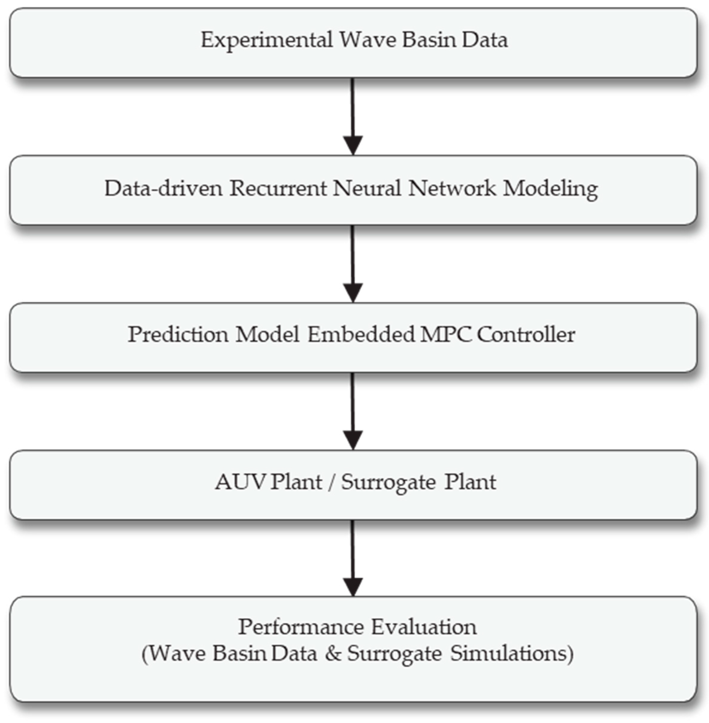
The overall research workflow, illustrating the stages from experimental data acquisition to data-driven modeling and robustness evaluation, is summarized in Figure 1.
The main contributions of this study to the literature are summarized as follows:
  • An LSTM-based data-driven prediction model representing the dynamic behavior of an AUV under wave effects has been developed using real measurement data obtained from experiments conducted in a wave basin.
  • The developed LSTM prediction model has been integrated into an MPC framework, enabling a more realistic evaluation of the effects of external disturbances such as waves and currents over the prediction horizon.
  • The behavior of the control structure trained under regular wave conditions was examined under irregular wave scenarios with characteristics not used during training, and the generalization performance of the proposed approach was assessed using experimental data obtained under these unseen wave conditions.
  • The stabilize mode of a Pixhawk (3D Robotics, Chula Vista, CA, USA)/ArduSub (Version 4.1.0)-based flight control system has been used for safe data acquisition during wave basin experiments and the collected measurements have been utilized for training and evaluating the LSTM-based prediction model.
  • While the LSTM model trained under regular wave conditions is employed within the control loop, a separate LSTM model trained using irregular wave data is utilized as a data-driven surrogate plant representation [10,11,12].
This separation enables systematic robustness evaluation under non-deterministic wave perturbations not explicitly included during controller training.
The proposed approach has been evaluated using wave basin measurement data incorporating realistic sensor noise and actuator constraints observed during the experiments, demonstrating the potential of data-driven control methods for practical and realistic AUV operating scenarios.

2. Experimental Platform and Data Collection Setup

In this section, the experimental platform used in the study, the data acquisition procedure, wave scenarios, data processing steps and the methodological details of the proposed data-driven control approach are presented. The aim of this section is to clearly and reproducibly define the different stages of the study, thereby enabling the obtained results to be reproduced and further developed by other researchers. Within this scope, the wave basin experiments conducted for data collection, the Pixhawk/ArduSub-based data acquisition process, the development of the LSTM-based prediction model and the integration of this model into the MPC framework are explained in detail.

2.1. AUV Platform and Onboard Control Architecture

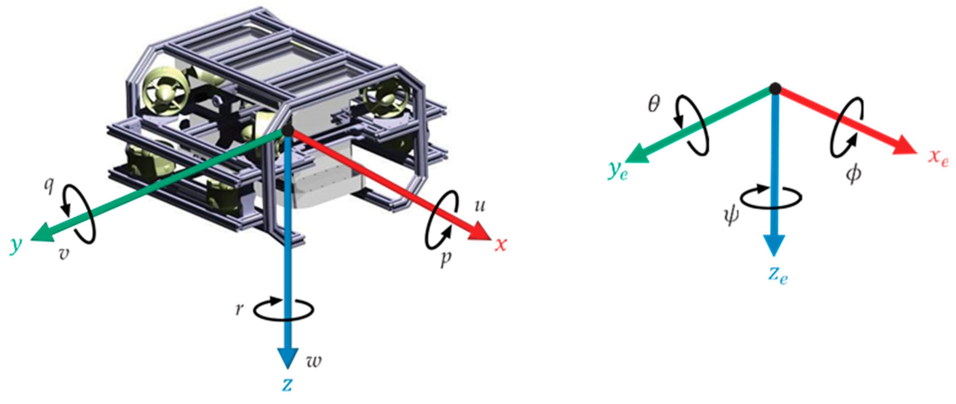
In this study, the body-fixed coordinate system of the AUV platform is defined based on the North–East–Down (NED) reference frame, which is widely adopted in the marine vehicles literature. This coordinate definition is selected to be directly compatible with the Pixhawk/ArduSub-based navigation and state estimation architecture, ensuring consistent transfer of velocity and attitude information obtained from onboard sensors to the modeling and control layers. The relationship between the body-fixed axes and the NED reference frame is illustrated schematically in Figure 2, while the symbols and notations used throughout the study are summarized in Table 1.

2.1.1. AUV Mechanical Structure

The experimental AUV platform employed in this study was custom-developed within the scope of the doctoral research rather than using a commercial off-the-shelf system. This approach allowed the realization of a dedicated experimental platform tailored for systematic investigation of modeling, prediction, and control strategies under controlled wave-basin conditions.
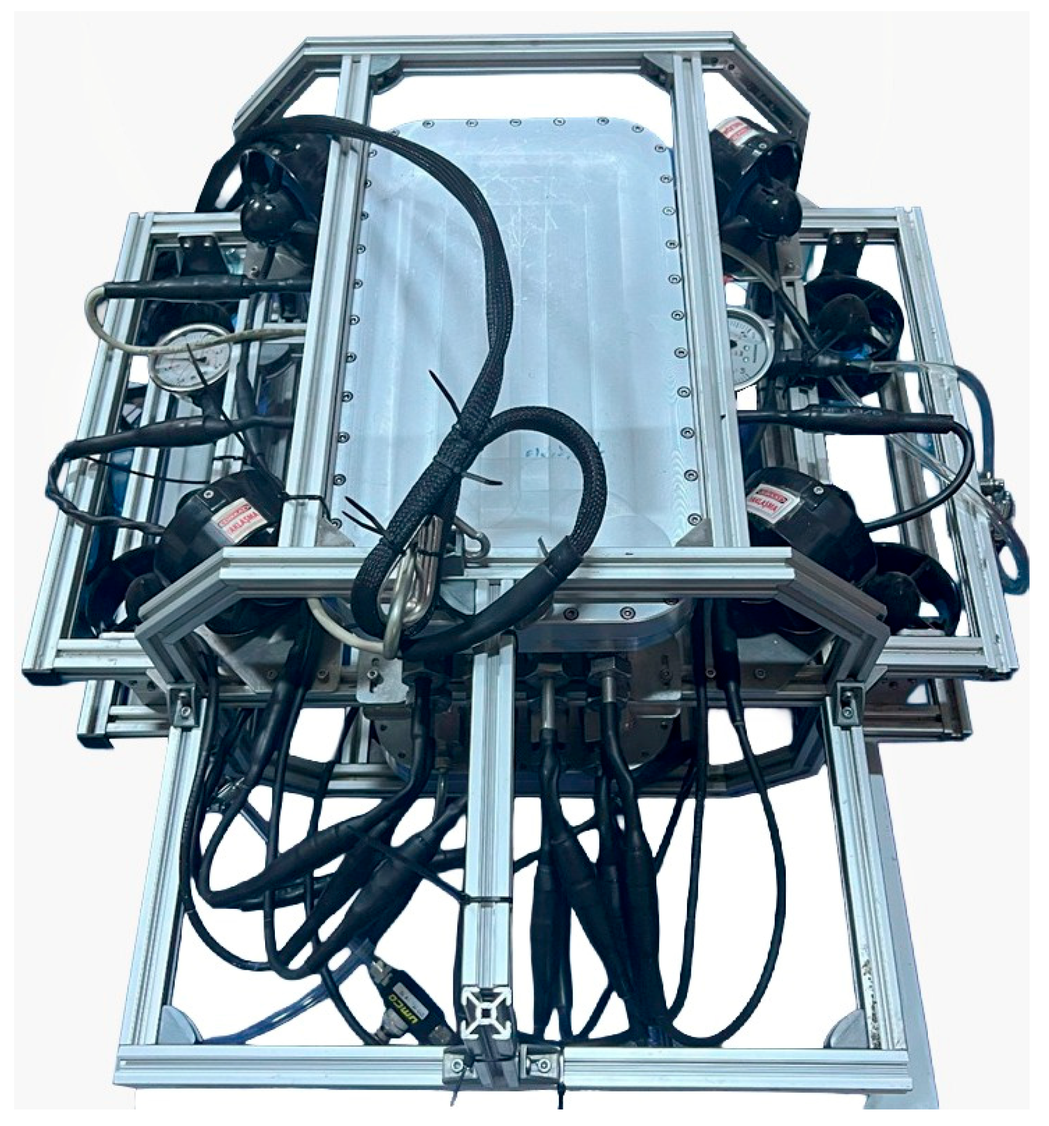
The mechanical structure adopts a BlueROV2-like modular architecture [13], which provides a compact and robust configuration suitable for near-surface operations. The vehicle is specifically configured to investigate velocity and attitude stabilization problems under wave-induced disturbances. Similar BlueROV2-type platforms are widely utilized in experimental validation of underwater control algorithms in both laboratory and open-water environments [14,15,16]. The developed AUV platform is shown in Figure 3.

2.1.2. Thruster Configuration

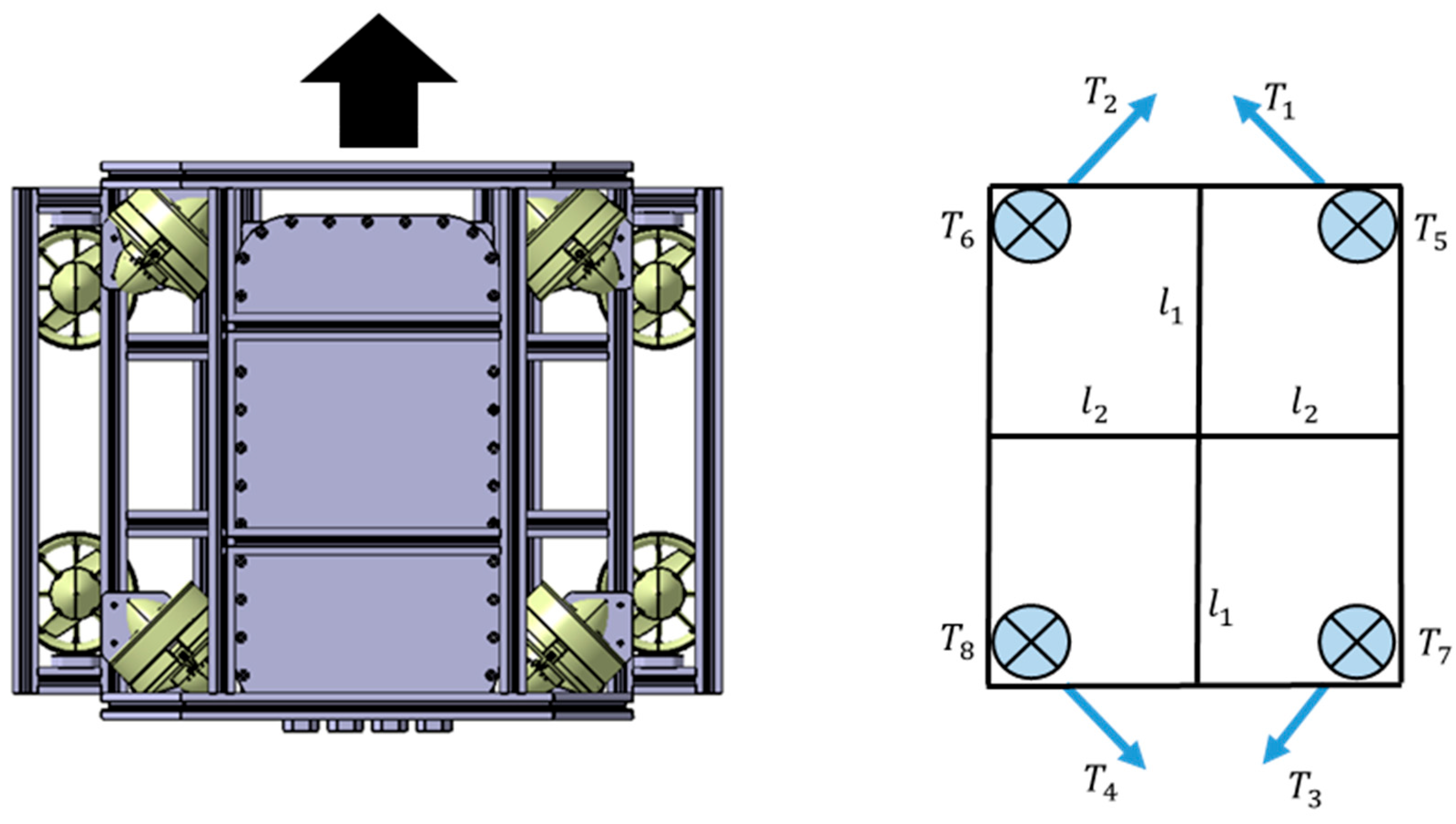
The developed platform features an eight-thruster propulsion configuration arranged to enable effective force and moment generation along all principal axes. The symmetric placement of horizontal and vertical thrusters allows over-actuated control in six degrees of freedom, enhancing disturbance rejection capability under wave conditions.
Over-actuated AUV architectures are widely adopted in the literature due to their advantages in station-keeping and disturbance rejection tasks [17]. Within MPC-based control frameworks, actuator redundancy can be incorporated directly into the optimization problem through appropriate thrust allocation strategies [18]. The thruster layout of the developed AUV is illustrated in Figure 4.

2.1.3. Buoyancy Adjustment and CG–CB Balancing

Prior to the wave basin experiments, the hydrostatic equilibrium of the vehicle was adjusted to ensure a repeatable near-surface operating condition. The relative CG–CB positioning was tuned to achieve a neutrally stable configuration in pitch and roll. Such buoyancy balancing is a common practice in experimental AUV and ROV studies to reduce modeling uncertainties and static offsets during controlled testing [19]. This procedure was conducted to establish a consistent experimental baseline and to minimize static offsets during data collection. Detailed mechanical illustrations are provided in Appendix Hydrostatic Configuration and Buoyancy Adjustment.

2.1.4. Sensors, State Estimation and Pixhawk/ArduSub-Based Control Architecture

On the AUV platform, the primary navigation sensors were integrated with the Pixhawk/ArduSub-based control architecture in order to observe the dynamic state of the vehicle and to carry out the experimental data collection process. Angular rates and linear accelerations are measured via the onboard IMU, while depth information is provided by the pressure sensor. Information related to the vehicle’s velocity and orientation is obtained by processing the measurements acquired from these sensors through sensor fusion and state estimation techniques [20].
The Pixhawk/ArduSub architecture utilizes an internal Extended Kalman Filter (EKF) framework for real-time sensor fusion. This internal EKF ensures the vehicle’s operational stability by providing precise and filtered state estimates to the low-level control loops, even under the challenging conditions of a wave basin. By leveraging this robust onboard estimation, the Pixhawk/ArduSub system functions as a reliable data acquisition and stabilization unit, ensuring experimental safety while maintaining the vehicle’s structural integrity during data collection. The use of such open-source flight control systems for high-fidelity experimental research on AUV and ROV platforms is well-documented in the literature [20].
Within the scope of this study, the Pixhawk/ArduSub controller was operated in Stabilize Mode during the wave basin experiments to establish a robust baseline. This mode employs low-level PID loops to maintain the vehicle at a zero-degree attitude (roll, pitch and heading), which inherently implies a target of zero for angular velocities (p, q, r). However, the controller does not actively manage the vehicle’s translational velocities (u, v, w) or position in a closed-loop [21]. The primary motivation for this configuration was to ensure operational safety while preventing the onboard controller from suppressing velocity variations. Consequently, the vehicle’s linear response was driven solely by hydrodynamic disturbances, allowing the effects of wave-induced forces to be directly observed and recorded. This approach provided the unbiased and repeatable experimental data necessary for the subsequent development of learning-based modeling and 6-DOF control strategies.
Prior to the experimental studies, Pixhawk sensor calibrations and system initialization procedures were performed via QGroundControl (Version 5.0.8) in order to ensure the consistency and repeatability of the recorded data [22]. System arming and disarming operations, as well as flight mode selection, were also conducted through the QGroundControl interface, which enabled real-time monitoring of the vehicle states during the wave basin experiments. All experimental data were logged by the Pixhawk flight controller and subsequently extracted using the Mission Planner (Version 1.3.82) software [23].

2.2. Wave Basin Setup and Experimental Conditions

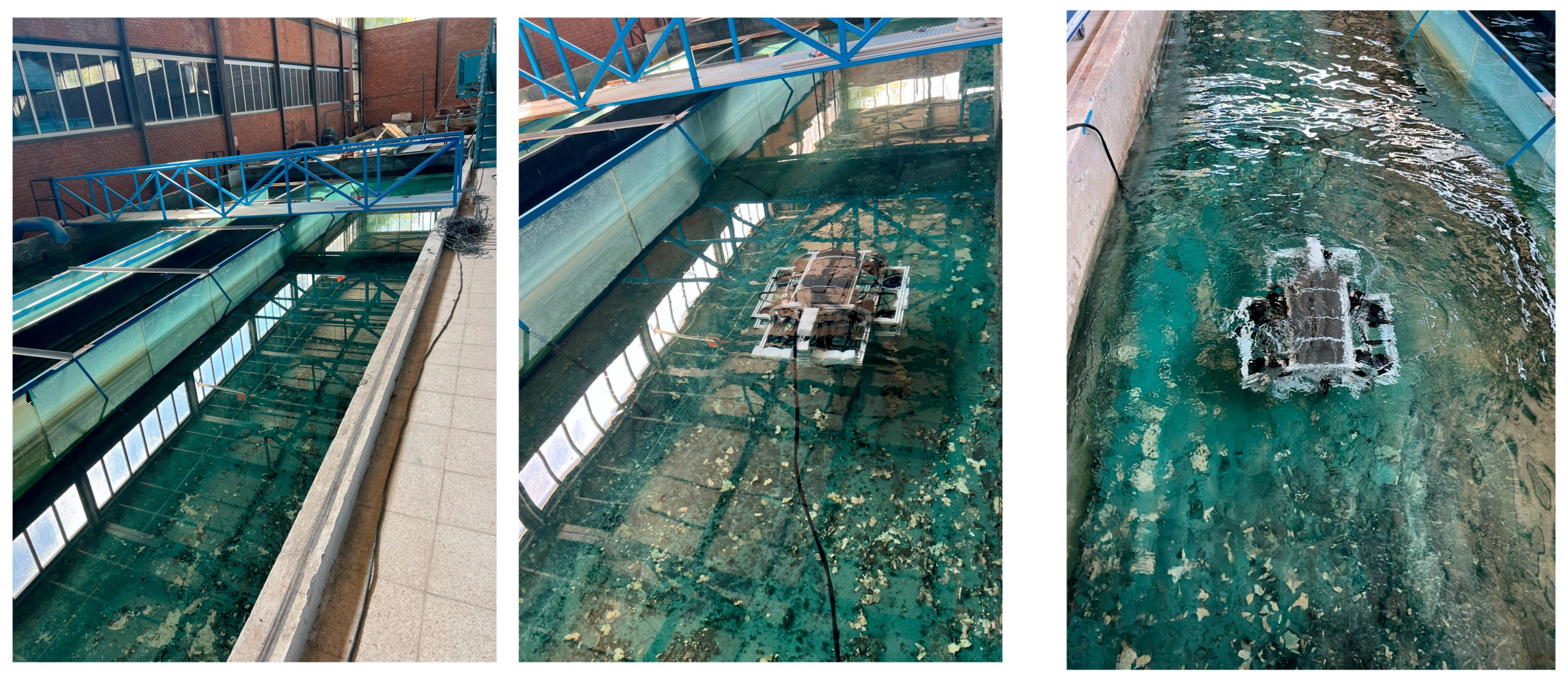
The experimental studies were conducted in a wave basin environment in which wave parameters could be generated in a controlled and repeatable manner. The wave basin was configured to enable the investigation of the dynamic behavior of autonomous underwater vehicles (AUVs) operating under wave-induced disturbances in near-surface conditions. The basin is equipped with a mechanical wave generator capable of producing unidirectional waves and the wave amplitude and frequency can be adjusted according to the experimental scenarios (Figure 5).
In this study, regular and irregular wave scenarios were generated in order to investigate the behavior of the AUV under different disturbance characteristics induced by waves. The water depth in the channel is 0.7 m. Three wave gauges are installed along the channel and the distance between the gauge closest to the vehicle and the AUV is 1 m.
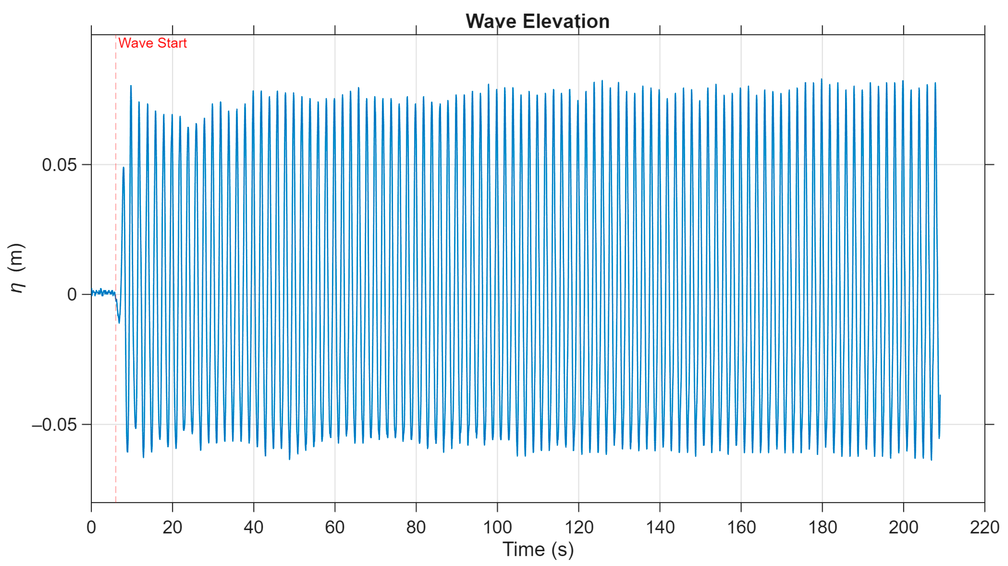
Regular wave conditions were generated using periodic wave profiles with a single dominant frequency and amplitude. These scenarios were selected to examine the fundamental dynamics of wave–vehicle interaction and the repeatable response characteristics of the system. Regular wave conditions also provide a controlled reference environment for training data-driven prediction models. In this study, regular waves were generated with a period of 2 s and a total of 100 wave cycles (Figure 6).
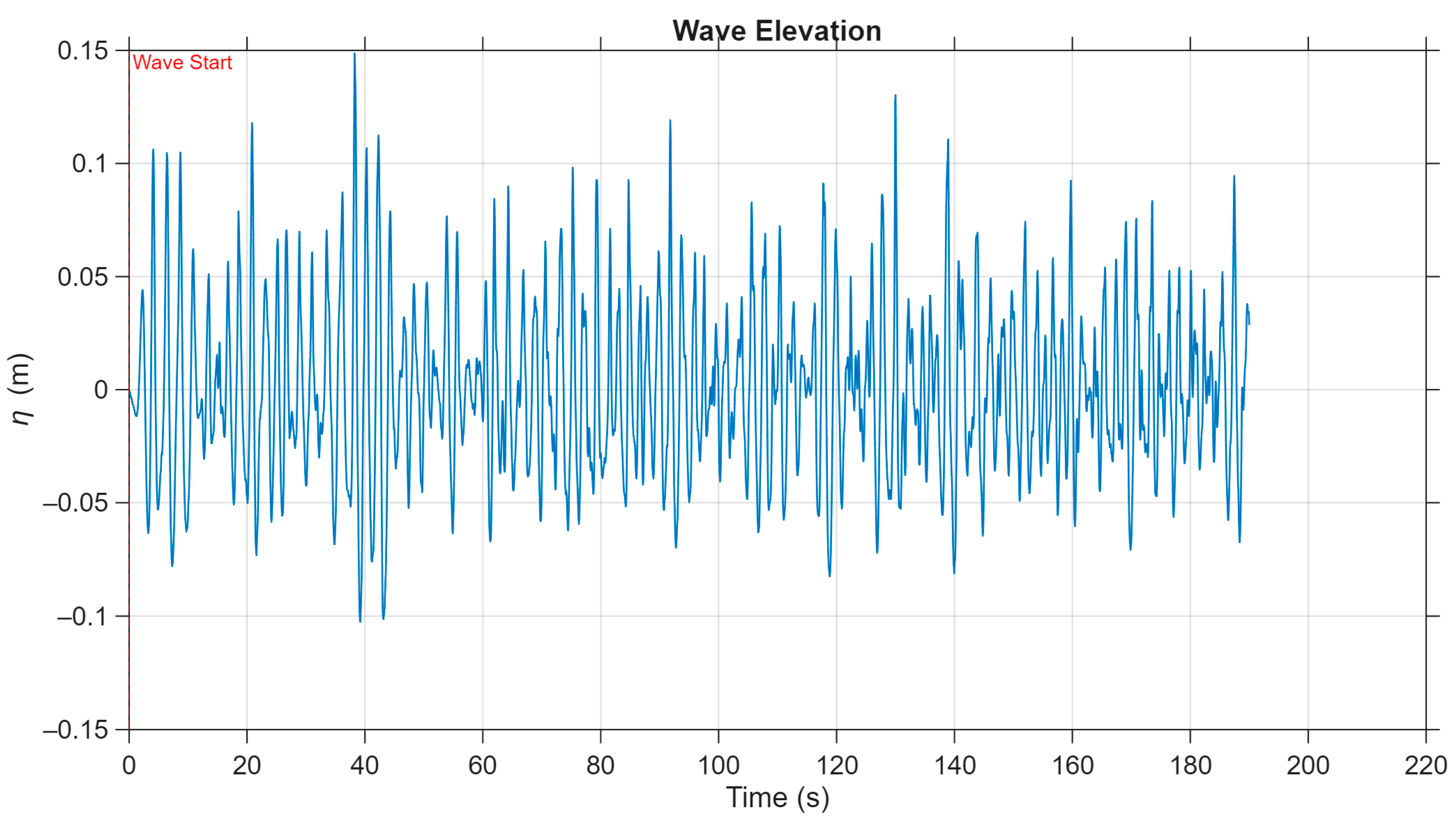
Irregular wave conditions were generated using wave profiles with time-varying amplitude and period characteristics, formed by the superposition of multiple frequency components [24]. The irregular waves were produced with a significant period of 2 s and a total of 100 waves (Figure 7).
These scenarios include broadband and less predictable disturbance effects that more accurately represent real sea conditions. Irregular wave conditions were used to evaluate the generalization capability of the proposed approach and its performance under unexpected environmental variations.

2.3. Experimental Data Logging and Preprocessing

During the experimental studies, the fundamental input–output signals representing the dynamic behavior of the AUV platform under wave disturbances were recorded through the Pixhawk/ArduSub-based control architecture. The data acquisition process aimed to obtain consistent, repeatable and time-synchronized datasets that could be used in learning-based prediction and control studies.

2.3.1. Logged Signals

The main signals recorded throughout the experiments are summarized below:
  • Thrust commands (PWM/thrust commands):
PWM-based thruster commands were recorded at a sampling frequency of 10 Hz, reflecting the effective command update rate of the control system. These signals represent the actuator-level control inputs of the vehicle.
  • Linear and angular velocity components:
The linear velocities in the vehicle body frame (u, v, w) were computed by transforming the North-East-Down (NED) velocity components—recorded via Pixhawk/ArduSub logs—into the body coordinate system using the corresponding orientation angles ( ϕ ,   θ ,   ψ ). Regarding the angular velocity components (p, q, r), these were not extracted from the internal EKF outputs due to logging constraints; instead, they were derived directly from the high-frequency raw gyroscope (GYR) measurements.
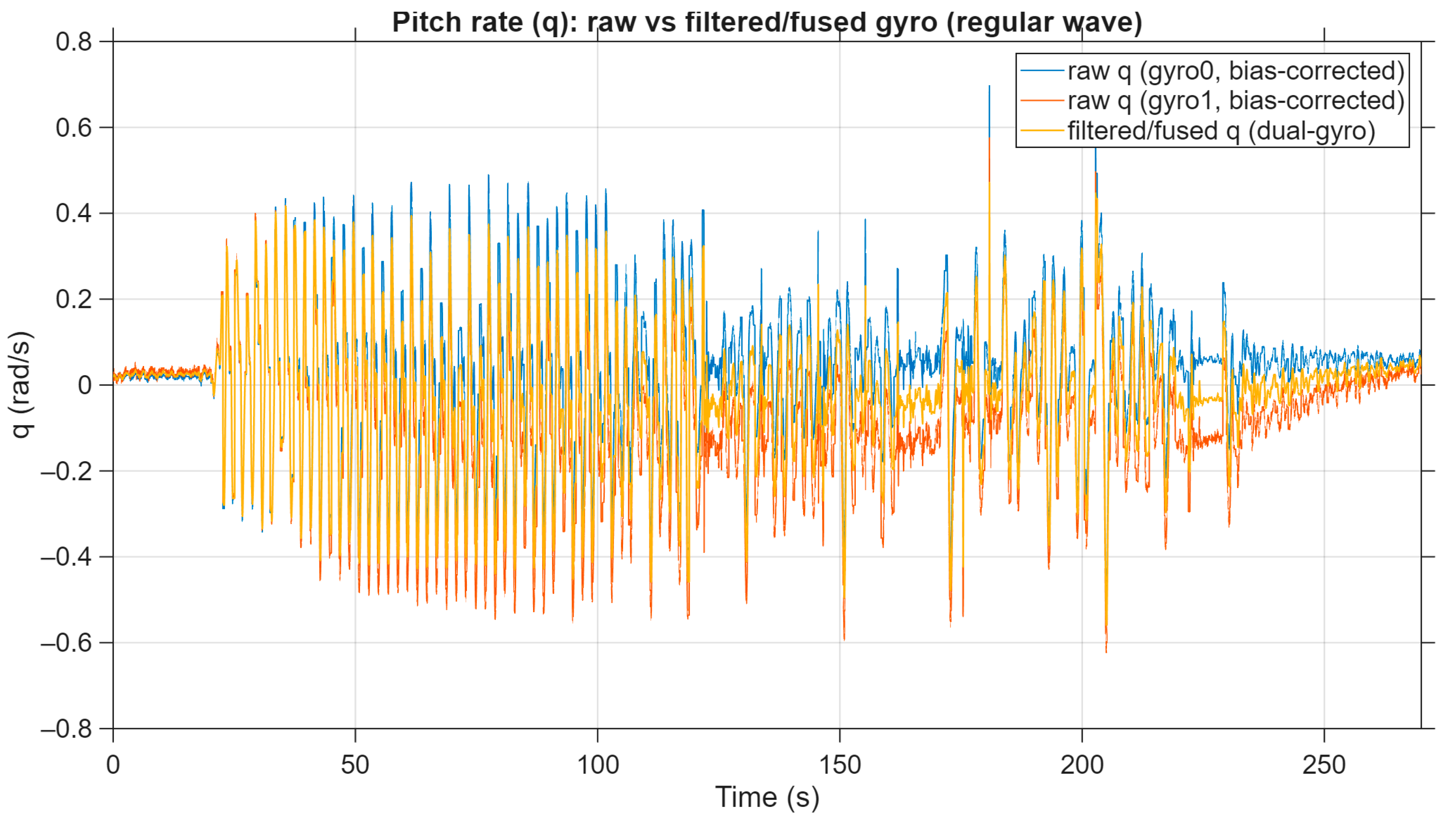
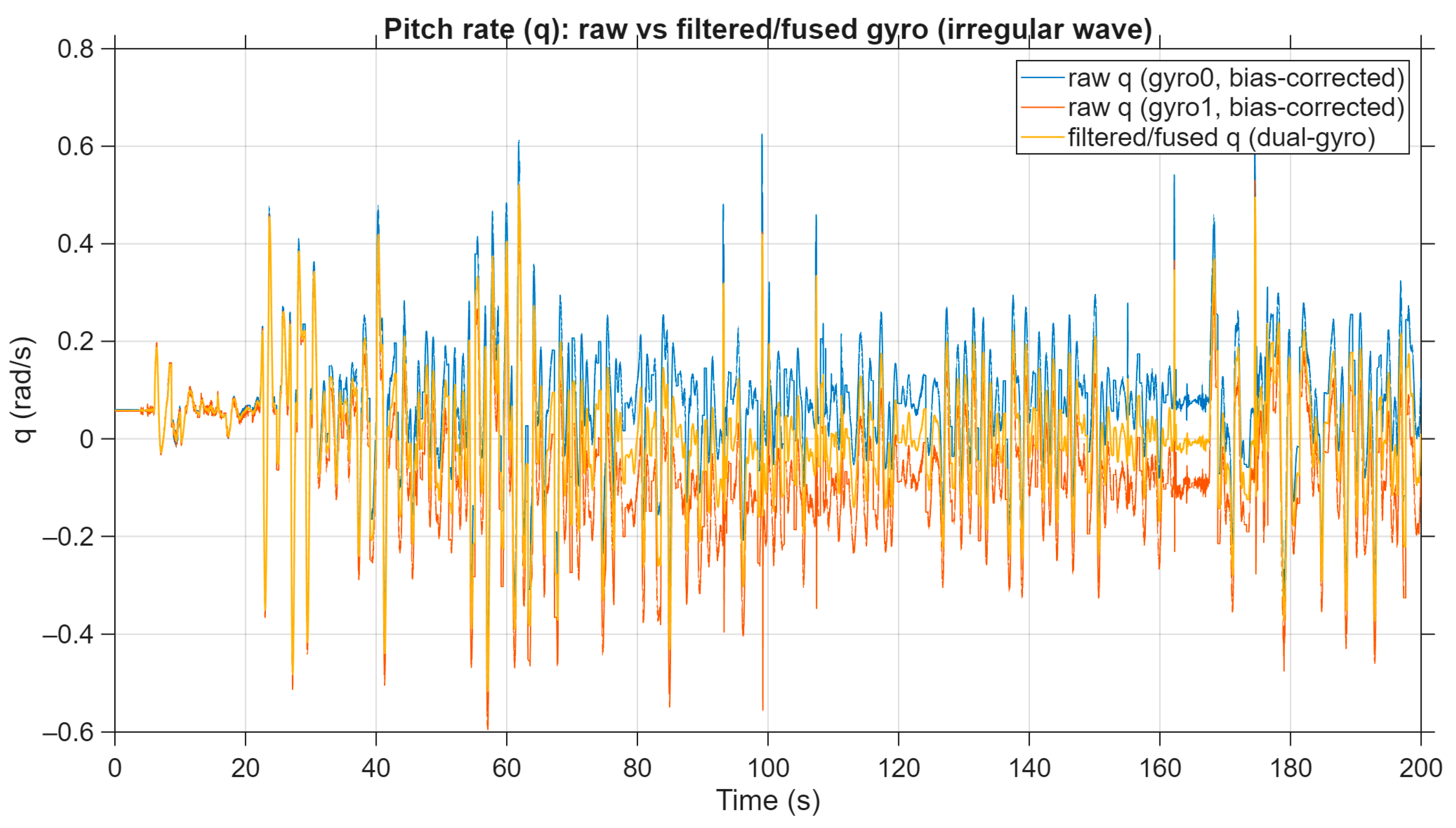
These signals were recorded at 100 Hz. To ensure data quality, these angular rate components were processed through bias correction and the fusion of multiple IMU measurements into a single, synchronized angular velocity time series. This procedure yielded a consistent 6-DOF velocity dataset representing the vehicle’s dynamic response to wave conditions. For instance, the transition from raw to filtered q angular velocity signals is illustrated in Figure 8 and Figure 9.
All signals were recorded continuously at a fixed sampling time throughout the experiments. The recorded datasets were labeled separately according to the regular and irregular wave scenarios.

2.3.2. Control Allocation and Axial Command Reconstruction

During the experiments, the Pixhawk/ArduSub controller generates PWM-based thrust commands through eight thrusters. Since the vehicle architecture is over-actuated, these PWM signals do not correspond one-to-one with the axial control inputs of the six degrees of freedom.
Therefore, in order for the experimental data to be used for modeling and control purposes, the thruster-level PWM commands were converted into equivalent control commands corresponding to the body-fixed axes. This conversion was performed using a constant control allocation matrix defined based on the geometry of the experimental platform and the thruster configuration.
First, the PWM signals for each thruster were centered around the neutral thrust value (Equation (1)).
P W M i = P W M i P W M m i d
Subsequently, these deviations corresponding to the eight thrusters were transformed into six axial control commands, u c t r l , through a linear mapping as expressed in Equation (2).
u c t r l ( 6 × 1 ) =   1 1 1 1   0 0   0   0 1 1 1   1   0 0   0   0   0 0   0   0   1 1   1   1   0 0   0   0 1 1 1   1   0 0   0   0   1 1 1 1 1 1   1 1   0 0   0   0 P W M ( 8 × 1 )
The matrix given here represents the control allocation matrix that describes the contribution of each individual thruster to the surge, sway, heave, roll, pitch and yaw axes. The resulting axial commands provide an input vector that represents the actual actuator-level behavior while being more suitable for control and learning algorithms.
The six axial control commands obtained in this manner constitute the input signals used in subsequent stages within the LSTM-based modeling and MPC framework.

3. Data-Driven Modeling Using LSTM

In this section, LSTM-based data-driven models developed using real measurement data obtained from wave basin experiments are presented. In the proposed approach, learning-based modeling is not limited solely to representing the approximate plant behavior of the system; instead, it is structured to investigate the robustness of the prediction and control components used within the MPC loop under different wave conditions.
Within this scope, two different LSTM models are defined:
  • An LSTM model trained under regular wave conditions and used within the control loop.
  • An LSTM-based plant prediction model trained under irregular wave conditions to represent the dynamic behavior of the system.
This separation aims to systematically evaluate the generalization capability of the proposed approach and its robustness against varying wave conditions.

3.1. Problem Formulation

In this study, the data-driven modeling approach is considered with the aim of obtaining a model that can approximately represent the complex and nonlinear dynamic behavior of an AUV under wave-induced disturbances. Since classical physics-based models are insufficient to fully capture the uncertainties and high-frequency dynamics that arise under surface wave effects, learning the system behavior directly from data is targeted.
For LSTM model training, a unified sampling rate was required to ensure temporal consistency between control inputs and system responses. Since the thruster PWM commands were available at 10 Hz, the sensor measurements originally recorded at 100 Hz were down-sampled to 10 Hz prior to training. Accordingly, the LSTM input–output sequences were constructed at an effective sampling frequency of 10 Hz, consisting of six-axis control commands and corresponding body-frame velocity measurements. This preprocessing step allows the LSTM model to learn the causal relationship between control actions and vehicle dynamics at the control-relevant time scale.
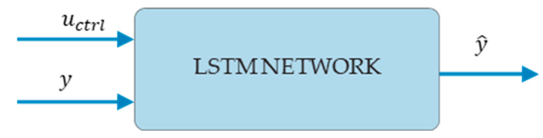
Within this scope, the problem is defined as a discrete-time one-step-ahead velocity prediction problem. The input vector of the LSTM-based model is constructed from time series that include past control inputs and vehicle velocity states. For each time step, the input vector consists of the following components:
  • The six axial control commands, u c t r l , corresponding to the surge, sway, heave, roll, pitch and yaw axes,
  • The past linear and angular velocity components measured in the vehicle body frame, y
With this structure, a total of a 12-dimensional input vector is provided to the LSTM network. The output of the model is the vehicle body-frame velocities at the next time step, y ^ , and the prediction of the six-dimensional velocity vector (u, v, w, p, q, r) is targeted. The overall input–output structure of the LSTM-based predictor used in this study is illustrated in Figure 10.
The LSTM input vector consists of the reconstructed six-axis control commands obtained through the control allocation process described in Section 2.3.2, together with the corresponding body-frame velocity measurements. The network output is defined as the predicted body-frame velocity vector at the next sampling instant.
In this approach, the LSTM network is not employed to construct a complete physical representation of the system; instead, it is used as a plant approximation that learns the causal relationship between the control inputs and the dynamic response of the vehicle. The ability of the LSTM to capture long-term dependencies provides a particular advantage in modeling the time-distributed dynamic effects induced by wave disturbances.

3.2. LSTM Network Architecture

In this study, a recurrent neural network (RNN) architecture based on LSTM cells was developed to model the dynamic responses of the AUV. The employed network structure was deliberately designed as a simplified architecture in order to keep the computational burden limited and to ensure usability within the control loop.
The developed LSTM network consists of three main layers:
  • Sequence Input Layer
  • LSTM Layer
  • Fully Connected (FC) Layer
The sequence input layer enables the time-series data to be processed appropriately by the network and allows the past input–velocity window to be fed into the network input. In this study, a fixed-length input window is used to facilitate learning of the short- and medium-term dynamic behavior of the system.
The LSTM layer is a specialized RNN structure capable of learning long-term dependencies in time-dependent data. Unlike conventional neural networks, the LSTM architecture incorporates a cell state and gate mechanisms that allow past information to be retained or selectively forgotten when necessary. This property makes LSTM particularly suitable for modeling disturbances such as wave effects that are distributed over time [25].
The forget gate determines how much of the information from the previous cell state is retained (Equation (3)).
f t = σ ( W f h t 1 , x t + b f
Here, f t denotes the output of the forget gate. h t 1 represents the hidden state from the previous time step and x t is the current input.
The input gate controls the extent to which new input information is added to the cell state (Equation (4)).
i t = σ W i h t 1 , x t + b i
Here, i t denotes the output of the input gate. Following the output of this gate, the new information to be added to the cell is computed using the hyperbolic tangent (tanh) activation function (Equation (5)).
C ~ t = t a n h ( W c h t 1 , x t + b c
Cell state update:
C t = f t C t 1 + i t C ~ t
Here, C t represents the current cell state, while C t 1 denotes the previous cell state.
The output gate determines the hidden state that will be propagated to the next time step (Equations (7) and (8)).
o t = σ ( W o h t 1 , x t + b o
h t = o t t a n h ( C t )
Through this gating structure, the LSTM network is able to retain meaningful historical information that influences the system dynamics, while suppressing irrelevant or noise-induced components. The output obtained from the LSTM layer is then passed through a fully connected layer, where a linear transformation is applied to produce the predicted velocity vector at the next time step, y ^ (Equation (9)).
y ^ = W × l a y e r o u t + b
This simplified architecture is designed to enhance generalization capability by avoiding excessive complexity, while also ensuring suitability for real-time control applications.

3.3. Training Strategy and Hyperparameter Optimization

In this study, the LSTM-based data-driven modeling approach was not limited to a single training scenario; instead, regular and irregular wave conditions were deliberately separated and utilized for two distinct purposes.
The experimental dataset obtained under regular wave conditions was used to train the LSTM model employed within the control loop. This model represents the nominal plant approximation used by the controller. In contrast, a second LSTM model trained using irregular wave data was considered as a generalized plant model representing the system behavior under more uncertain conditions requiring a stronger generalization capability. Through this separation, the robustness of the proposed control approach against variations in the wave spectrum could be systematically investigated.
Prior to training, all input and output signals were subjected to Z-score normalization using the mean and standard deviation values computed from the training dataset. This normalization aims to ensure balanced contributions of signals with different physical magnitudes and units to the learning process and to promote more stable operation of gradient-based optimization algorithms [26]. The Z-score normalization is defined as follows (Equation (10)).
x = x μ σ
Here, x ,   x ,   μ ,   σ denote the raw data, the normalized data, the mean and the standard deviation, respectively.
The dataset was divided sequentially based on temporal order without random shuffling. Specifically, the first 70% of the recorded time-series data were used for training, the subsequent 15% for testing, and the final 15% for validation. This chronological splitting strategy preserves the temporal dynamics of the wave-induced responses and prevents information leakage between subsets. No overlapping windows were shared across the training, testing, and validation datasets. Furthermore, normalization parameters were computed exclusively from the training subset and kept fixed during both testing and validation phases to eliminate any form of data leakage.
Both LSTM models were trained using an offline learning approach, and the mean squared error (MSE) was employed as the loss function during training. For the overall evaluation of the training results, mean absolute error (MAE) and root mean squared error (RMSE) metrics were used (Table 2). However, in safety-critical systems such as AUVs, standard expectation-based metrics may fail to account for tail risks—rare but large errors that can compromise system stability [27]. To provide additional statistical insight into extreme deviations, the Conditional Value-at-Risk (CVaR) metric was employed at a confidence level of α = 0.05 as a post-evaluation measure of robustness under stochastic wave disturbances [28]. It should be noted that CVaR is not incorporated into the MPC objective function nor used as a risk-aware control criterion; rather, it is used solely as a statistical performance metric. For our discrete test dataset, the empirical CVaR was calculated by averaging the top 100α% of the ordered absolute residuals [29]. These metrics (MAE, RMSE, and CVaR) were consistently applied to evaluate both the LSTM prediction accuracy and the closed-loop velocity tracking performance of the LSTM-MPC framework.
After training was completed, the network weights were frozen and directly used during the baseline control and evaluation stages, while online adaptation was investigated separately to improve robustness under increased noise and model degradation.
During the training of the LSTM network, the network weights were updated using the Adam optimization algorithm. By combining adaptive learning rates with momentum-based update mechanisms, the Adam algorithm provides stable and fast convergence when training recurrent neural networks with noisy time-series data. In this study, Adam optimization was applied offline for each training configuration using hyper-parameters determined via grid search.
The hyper-parameters of the LSTM networks were selected using a grid search procedure. Among the investigated parameters, the number of hidden units was varied between 16, 32, 64, 128 and 256 to evaluate model capacity and prediction performance. While larger architectures yielded slight improvements in certain offline validation metrics (see Appendix B.1, Table A1, Table A2 and Table A3), the performance gains diminished beyond 64 hidden units. To avoid bias due to controller tuning, Bayesian optimization of the MPC parameters was repeated for both the 64- and 128-unit LSTM predictors using the same search space and termination criteria. Despite retuning, the 128-unit configuration consistently resulted in a higher average MPC solve time, exceeding the adopted 10 Hz control update interval. Therefore, the selection of 64 hidden units was driven by computational compatibility rather than tuning-related effects.
More importantly, since the LSTM predictor is embedded within the MPC optimization loop and executed recursively at each control interval, computational efficiency becomes an important design criterion. For the adopted control frequency of 10 Hz, the optimization process is expected to remain compatible with the assumed sampling interval. Experimental evaluation indicated that the 128-unit LSTM increased the average MPC solve time to approximately 0.144 s per step, whereas the 64-unit configuration maintained an average solve time of approximately 0.026 s per step while preserving stable optimization convergence.
Therefore, model selection was performed based on a trade-off between prediction accuracy and computational compatibility with the control update interval. The 64-unit LSTM configuration provided the most balanced compromise between model capacity, generalization performance and computational efficiency, and was thus selected for integration into the control framework.
The upper limit for the number of training epochs was set to 50. Analysis of the training loss curves indicated that more than 90% of the total error reduction occurred within this range. Increasing the number of epochs beyond this limit did not result in meaningful improvements in prediction accuracy and instead increased computational cost. The mini-batch size was kept small to preserve temporal diversity in the time-series data and to enhance generalization capability and was set to 8. In addition, a cosine learning rate schedule was employed during training to gradually reduce the learning rate in a smooth and non-monotonic manner, which helped stabilize convergence and prevented oscillatory updates in the later stages of training, particularly for noisy time-series data (Table 3).
In this study, Huber Loss was utilized as the loss function. Huber Loss combines the advantages of MSE and MAE, providing a balanced approach toward both low and high error values. In low-error regions, it behaves quadratically like MSE, offering stability advantages. Conversely, in high error regions, it responds linearly like MAE, preventing outliers—such as sudden spikes in data—from disproportionately affecting the training process. This characteristic ensures a more robust learning process against sudden velocity changes and sensor noise, which are frequently encountered in LSTM-based prediction models operating under wave disturbances [30].
In addition to the LSTM configurations evaluated during the grid search, GRU architectures with 64 hidden units were trained under identical preprocessing, dataset partitioning, and training conditions to evaluate whether a simplified recurrent structure could provide comparable performance within the proposed MPC framework. The comparative results, summarized in Appendix B.2 (Table A4, Table A5 and Table A6), reveal that although the GRU model achieved similar one-step prediction accuracy under regular wave conditions, architectural differences became evident when recursive prediction behavior and disturbance generalization were considered.
Since the predictive model operates recursively within the MPC optimization loop, stability over the prediction horizon constitutes a fundamental control requirement. As shown in Table A5, the GRU exhibited higher error accumulation at the horizon end. Furthermore, under irregular wave excitation—representing unseen and broadband disturbance characteristics—the GRU demonstrated substantially larger degradation in both mean error and CVaR metrics compared to LSTM (Table A6).
These findings indicate that the explicit memory cell structure of the LSTM provides improved robustness in modeling long-horizon temporal dependencies and multi-scale disturbance dynamics. Therefore, the model selection was guided by a control-oriented evaluation emphasizing recursive stability and disturbance generalization rather than single-step prediction accuracy alone. Based on this combined assessment, the LSTM architecture with 64 hidden units was selected as the most suitable configuration for integration within the MPC framework.

4. Control Strategy

In this study, the velocity stabilization problem of an AUV operating under wave-induced disturbances is addressed within a Model Predictive Control (MPC) framework supported by a data-driven prediction model. MPC computes optimal control inputs over a finite prediction horizon by explicitly incorporating system dynamics and actuator constraints into an optimization problem [31,32]. This structure makes MPC particularly suitable for marine environments characterized by time-varying and partially unpredictable disturbances such as surface waves and currents [33].
Building upon the architecture selection discussed in the previous section, the analytical AUV dynamic model traditionally used within MPC is replaced by the selected LSTM-based data-driven predictor trained on experimental measurements. By embedding this learned nonlinear mapping into the control loop, the predictive model directly reflects observed system behavior, thereby reducing dependence on uncertain hydrodynamic parameters and mitigating plant–model mismatch effects.

4.1. LSTM-Based Control Framework

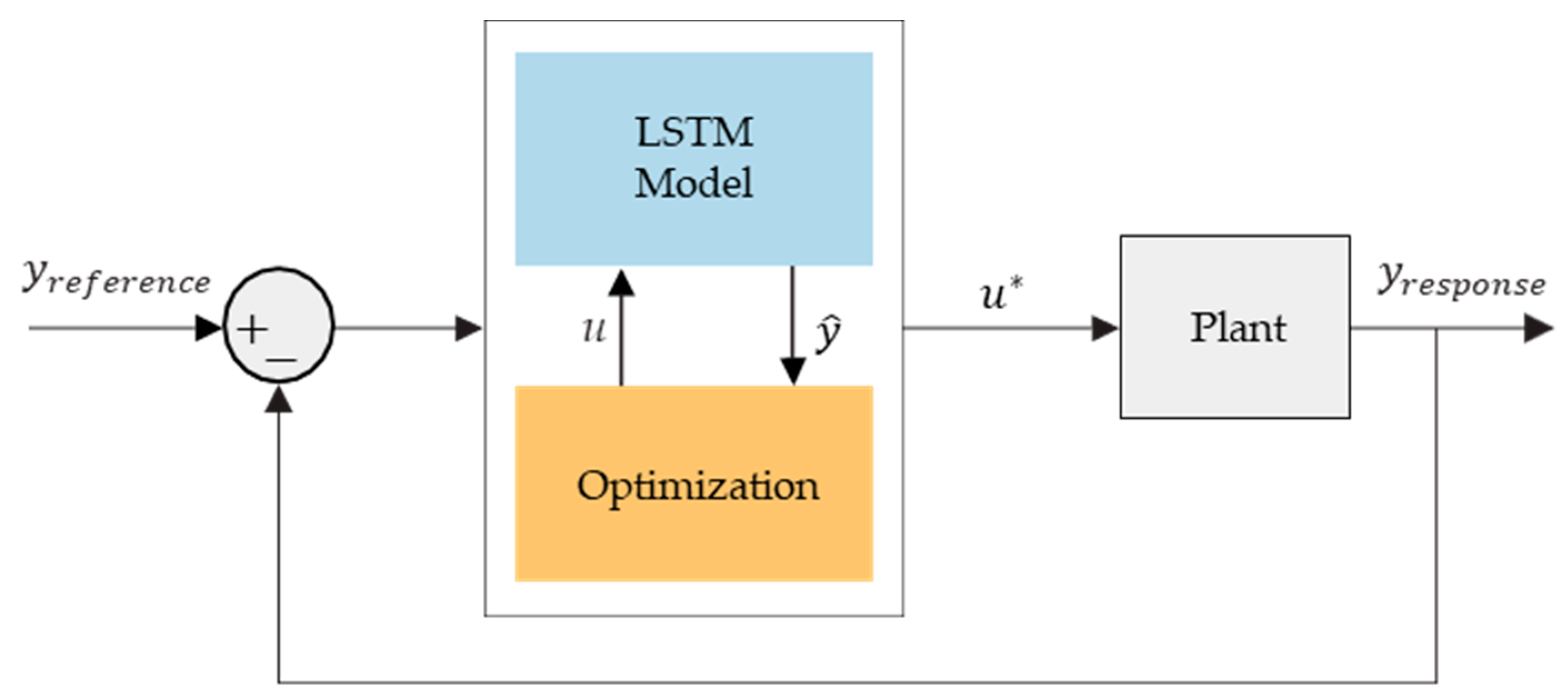
In the proposed control architecture, the LSTM network is not positioned as a direct controller, but rather as the predictive model used within the MPC framework. The LSTM network predicts the system’s velocity response at the next time step by using past control inputs and body-frame velocity measurements. These predictions are utilized within the MPC optimization loop to evaluate candidate control inputs.
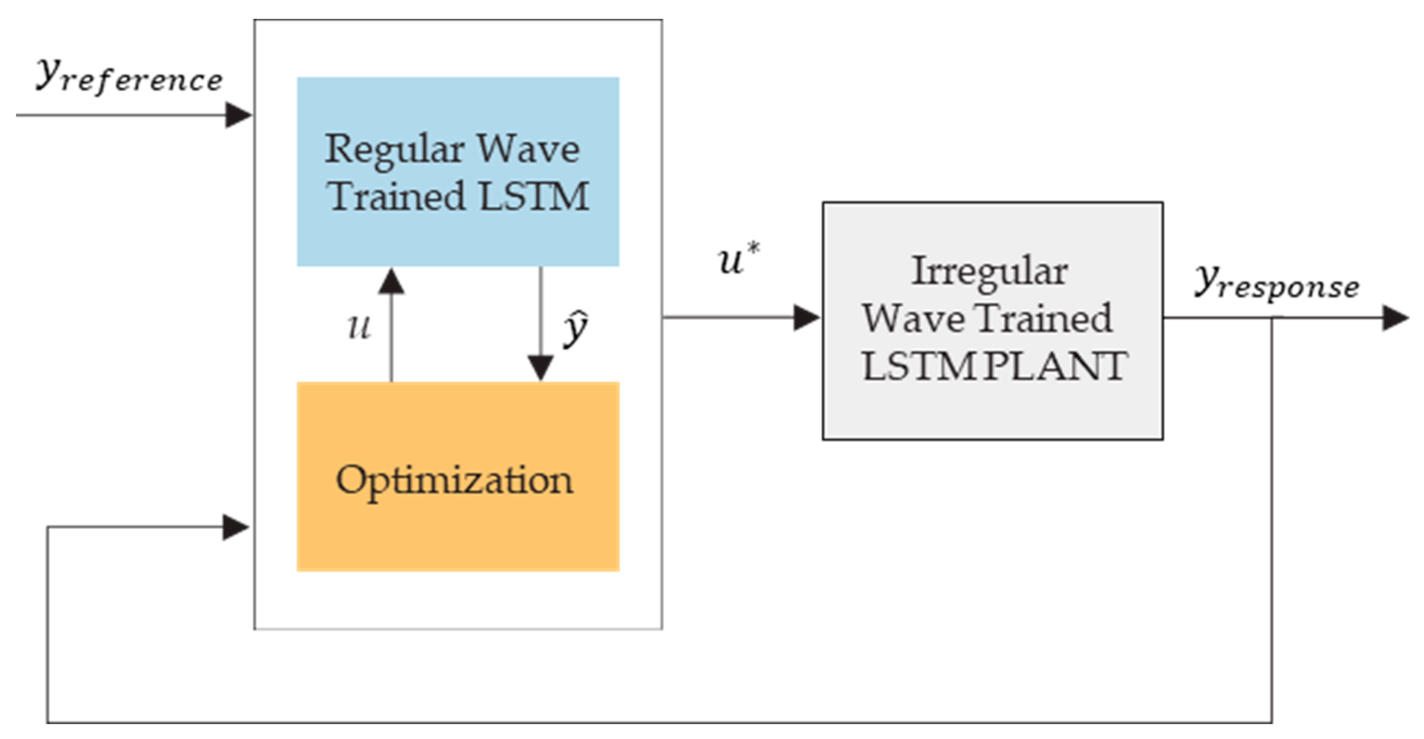
The overall structure of the proposed LSTM–MPC framework is schematically illustrated in Figure 11. This structure follows a classical MPC loop, in which the prediction, optimization and control application steps are repeated at each sampling instant.
The MPC loop was configured to operate at a sampling frequency of 10 Hz, matching the operating frequency of the LSTM-based prediction model. This choice ensures that the prediction horizon and the control update rate remain consistent with the temporal resolution of the learned dynamics. At each control step, the MPC optimization problem is solved, the first control input is applied following the receding-horizon principle and the process is repeated at the next sampling instant.
In the nominal control loop, the LSTM network operates with fixed weights that are trained offline using experimental data and no online learning or network update is performed during standard MPC operation. In this way, the learning process and the control implementation are explicitly decoupled. An online learning extension is investigated separately to enhance robustness under increased measurement noise and model degradation.

4.2. Controller Design

The MPC problem is formulated as a finite-horizon optimal control problem. At each control step t, the objective is to determine the optimal control sequence U given in Equation (11). This sequence minimizes the cost function J, subject to the state transition model defined in Equation (12) and the input constraints specified in Equation (13) for all i { 0 ,   ,   N 1 } , where N denotes the prediction horizon.
U = { u t ,   u t + 1 , ,   u t + N 1 }
y ^ t + i + 1 = f m o d e l ( y ^ t + i , u t + i )
u m i n u t + i u m a x
The primary objective of the controller is to regulate the six-degree-of-freedom body-frame velocity components (u, v, w, p, q, r) around their reference values while preventing abrupt variations in the control inputs. The cost function is defined in Equation (14). The control increment term appearing in Equation (14) is defined in Equation (15).
J = i = 1 N [ γ y ^ t + i y r e f t + i 2 + λ u t + i 2 ]
u t + i = u t + i u t + i 1
In the proposed framework, the analytical transition model f m o d e l in Equation (12) is replaced by a data-driven LSTM predictor expressed in Equation (16).
y ^ t + i + 1 = f L S T M ( y ^ t + i , u t + i )
This substitution embeds the nonlinear temporal dynamics captured by the LSTM directly into the MPC optimization loop. Therefore, the proposed approach preserves the classical MPC optimization structure while replacing the analytical state-transition function with a learned nonlinear mapping.
The resulting optimization problem is nonlinear due to the embedded LSTM predictor and is solved using Sequential Quadratic Programming (SQP) in MATLAB® (R2025a update 1) via the fmincon solver. The control inputs over the prediction horizon are directly treated as decision variables, and gradient information is obtained numerically.
The weighting coefficients (γ, λ) in the MPC cost function and the prediction horizon N are determined offline using Bayesian Optimization [34]. The resulting MPC parameters, including the prediction horizon and the weighting coefficients used in the cost function, are summarized in Table 4.
Bayesian optimization is not part of the online MPC solution process and is employed solely for tuning the control parameters, thereby avoiding any additional computational burden during real-time operation. An additional soft penalty term is introduced when control inputs exceed 85% of their admissible bounds.
The objective in determining the control parameters is not to achieve the theoretically minimum cost value, but rather to obtain a stable, non-saturating and real-time implementable control behavior under wave-induced disturbances. Therefore, the Bayesian optimization process is configured to terminate when the improvement between successive iterations of the cost function falls within a predefined tolerance range.
With this structure, the MPC provides a short-horizon and computationally efficient control framework that utilizes an LSTM-based nonlinear prediction model, enabling the regulation of AUV velocity dynamics under wave disturbances in a manner suitable for real-time applications.

5. Validation and Simulation Results

In this section, the performance of the proposed LSTM-based data-driven control approach is evaluated using data obtained from wave basin experiments. All results presented are obtained using LSTM models whose weights were frozen after the offline training and normalization procedures described in Section 3. The evaluations are carried out under both regular and irregular wave conditions.

5.1. LSTM Training Accuracy for Control and Plant Representation

In this section, the prediction accuracies of the two LSTM models used for control and plant representation purposes are presented separately. The objective is not to compare the models with each other, but to demonstrate whether each model provides sufficient accuracy for its intended role.
The LSTM model trained under regular wave conditions is designed to be used as the predictive model within the MPC framework. The purpose of this model is to represent the repeatable dynamics observed in the wave basin with sufficient accuracy.
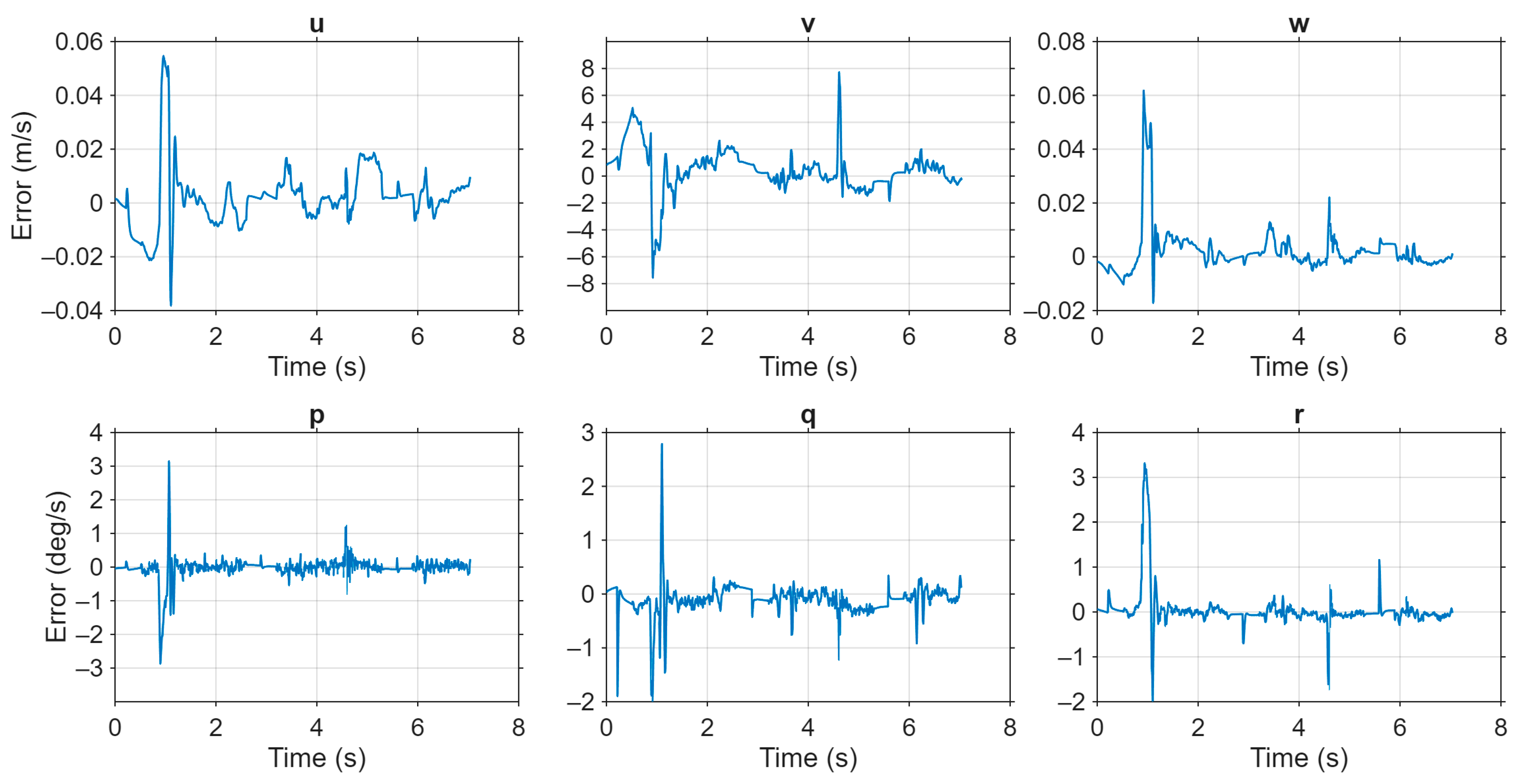
The prediction errors obtained along the six axes remain stable and bounded in the time domain (Figure 12). These results indicate that the LSTM model trained under regular wave conditions provides a sufficiently accurate nominal prediction model that can be reliably used within the MPC prediction horizon (Table 5). The regular-wave test dataset spans approximately 7 s, corresponding to three full wave periods (T = 2 s). Given the periodic and repeatable nature of regular waves, this duration is sufficient to capture both transient and steady-state prediction behavior. Therefore, the selected test window provides an adequate basis for evaluating the model’s suitability within the MPC prediction horizon. Furthermore, the calculated CVaR values across all degrees of freedom serve as a rigorous post-analytical benchmark for prediction reliability in the worst-case scenarios. Although the CVaR metrics are naturally higher than the MAE and RMSE due to their focus on tail-end distributions, they remain within acceptable operational limits. This confirms that even under peak disturbance fluctuations, the LSTM model maintains its robustness, demonstrating that extreme deviations are statistically contained and do not compromise the feasibility of the MPC optimization process.
The second LSTM model, trained using irregular wave data, is not used within the controller in this study; instead, it is considered as a test plant model representing more complex and broadband wave effects.
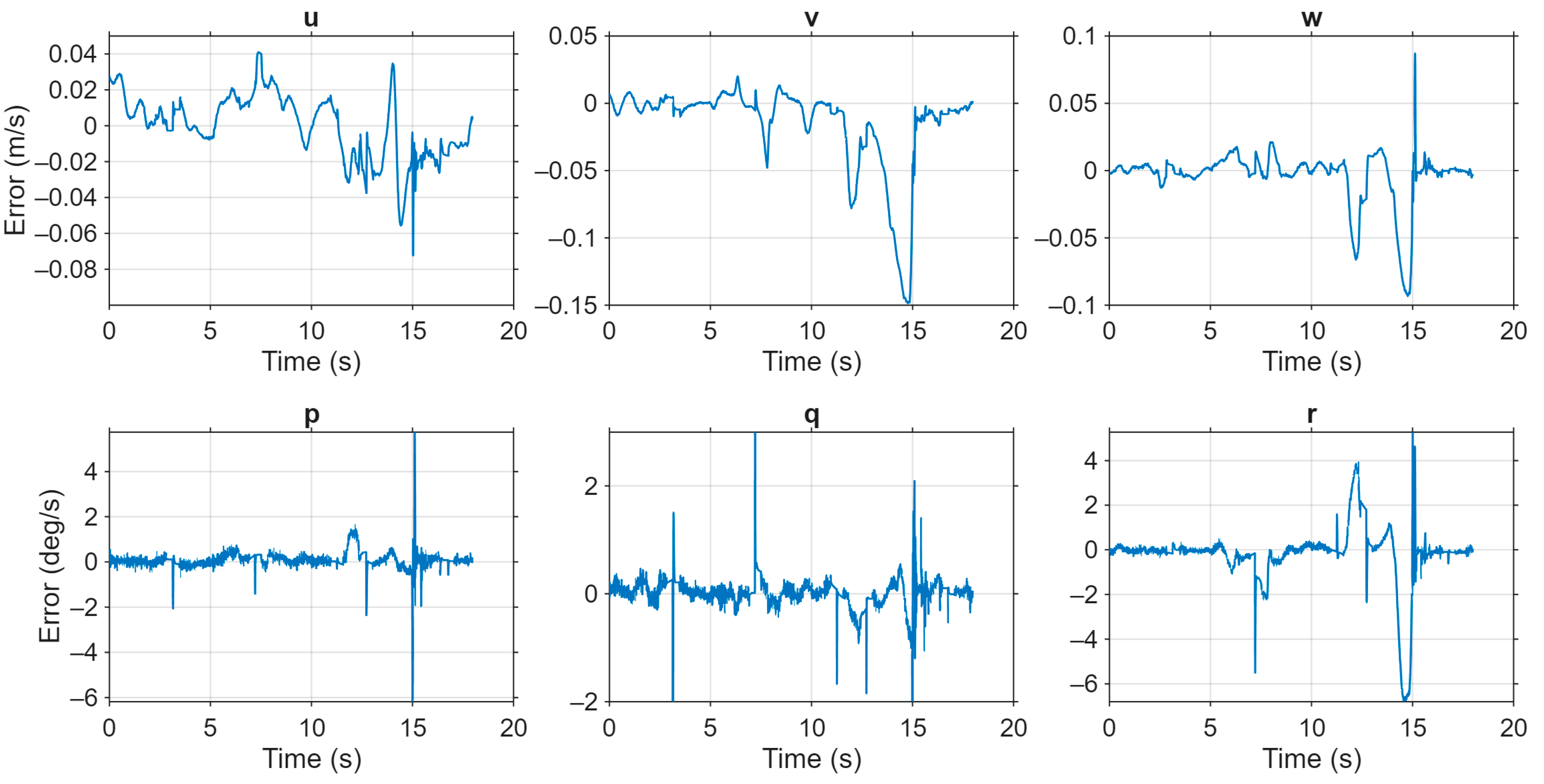
This model represents untrained and more uncertain dynamics from the controller’s perspective (Figure 13).
The quantitative error metrics are given in Table 6. In contrast to the regular-wave case, the irregular-wave test dataset spans approximately 18 s, corresponding to roughly nine dominant wave periods. Due to the stochastic and broadband characteristics of irregular waves, a longer evaluation window is necessary to capture variability across multiple wave realizations. This extended duration enables a more representative assessment of the surrogate model’s robustness under non-periodic disturbance conditions.
This model demonstrates high accuracy on experimental data, proving its reliability as a data-driven surrogate plant representation of real system behavior. Prediction errors across the six degrees of freedom remain stable and bounded in the time domain, even under the challenging stochastic conditions imposed by irregular waves (Table 6). Furthermore, the use of CVaR as an evaluation tool allows for a rigorous assessment of the model’s reliability in worst-case scenarios. For instance, the CVaR value of 5.3229 in the yaw axis under irregular waves clearly exposes extreme deviations that standard metrics such as MAE (0.6086) might otherwise mask. This analysis demonstrates that the errors produced by the surrogate model remain within statistically predictable bounds, providing a robust probabilistic boundary for the subsequent MPC optimization process.

5.2. Robustness Against Plant Mismatch Under Irregular Waves

To evaluate the robustness of the proposed framework under plant uncertainty, a series of mismatch tests was conducted by subjecting the controller to irregular wave conditions. In this scenario, the MPC utilizes an internal model trained solely on regular wave data (reg-LSTM), while the actual system behavior is represented by a surrogate plant trained on irregular wave data (irreg-LSTM). This setup, detailed in the flowchart in Figure 14, deliberately introduces a model-plant mismatch to simulate environmental variability.
The simulation maintains a dual-rate execution: the plant dynamics evolve at 100 Hz to capture high-frequency interactions, while the control updates are performed at 10 Hz, mirroring the practical constraints of experimental AUV hardware. Each simulation run was executed for a total duration of 50 s. To ensure physical consistency between the mismatched models, parallel normalization buffers are maintained. As illustrated in Figure 14, the control inputs and velocity histories are processed using separate Z-score parameters ( μ r e g , σ r e g and μ i r r e g , σ i r r e g ) before being fed into the respective LSTM blocks.
The core of this evaluation lies in the receding horizon strategy. At each step, the MPC optimizes the control sequence by predicting future responses through the reg-LSTM, yet the ‘ground-truth’ state update is provided by the irreg-LSTM. The optimization problem is solved using the Sequential Quadratic Programming (SQP) method, where the reg-LSTM is executed in a forward manner to evaluate candidate control inputs. By applying only the first step of the optimized sequence and resolving at each interval (Algorithm 1), the closed-loop system’s ability to stabilize the vehicle under intentional model inconsistency is systematically assessed.
Algorithm 1: LSTM-MPC Simulation Loop
Applsci 16 04187 i001
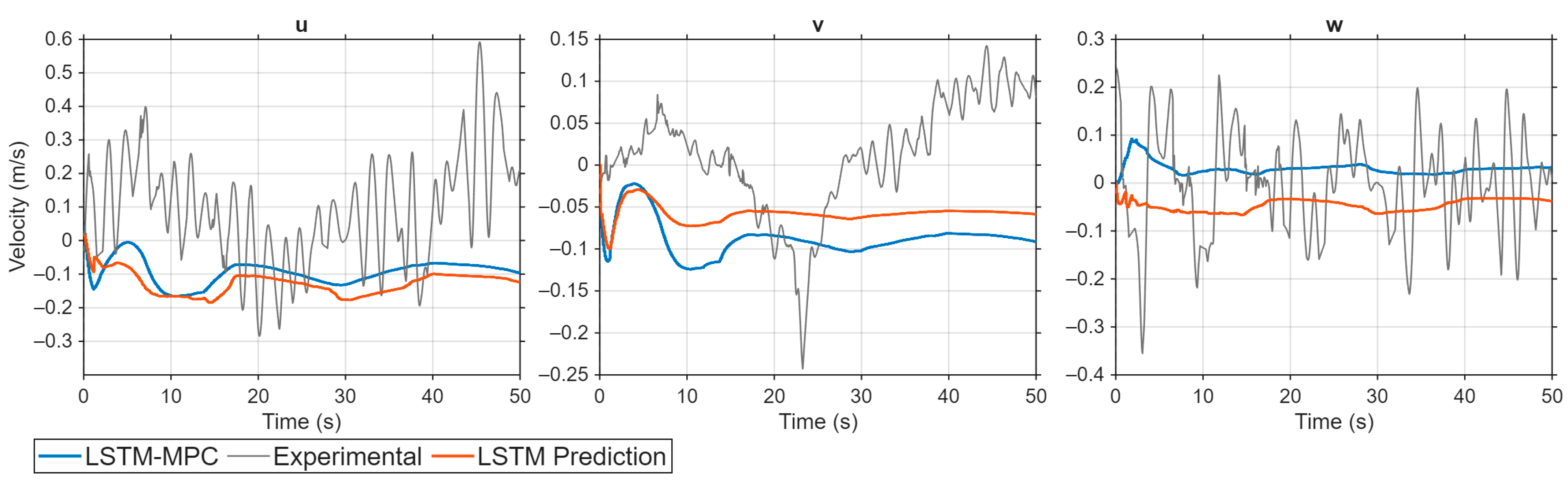
The robustness of the proposed LSTM-MPC framework was first evaluated in a noise-free simulation environment to isolate the effects of spectral plant mismatch. The primary objective was to determine if the controller could maintain a zero-velocity state (u, v, w, p, q, r = 0) despite the prediction model (reg-LSTM) having no prior exposure to the irregular wave dynamics of the plant (irreg-LSTM). The comparative 6-DOF velocity responses are illustrated in Figure 15 and Figure 16, while the detailed performance metrics, including MAE and RMSE for each axis, are summarized in Table 7.
According to the statistical data provided in Table 7, the LSTM-MPC successfully mitigates wave-induced disturbances even under significant model inconsistency:
  • Translational velocity stabilization: The most significant improvement was observed in the heave axis, where the MPC achieved an MAE of 0.0303 m/s, representing a 61.8% reduction compared to the experimental baseline (EXP).
  • Rotational rate control: The controller exhibited high effectiveness in stabilizing the roll (p) rate, reducing the MAE from 5.150°/s to 1.400°/s (a 72.8% improvement).
  • Prediction fidelity: The internal prediction accuracy of the LSTM remains high (e.g., u MSE: 0.0017), confirming that the model generalizes well to irregular wave patterns. However, it is observed that the prediction error for the yaw rate (r) is relatively higher compared to other axes, yielding an MSE of 7.0735. This increased error can be attributed to the persistent and stochastic nature of yaw drift induced by irregular wave encounters, which presents a more complex temporal pattern for the reg-LSTM to generalize.
  • CVaR-based extreme deviation analysis: The analysis of the metrics confirms that the EXP CVaR values, reaching 15.9741, particularly in the yaw axis, indicate that actual stochastic disturbances in the wave tank lead to severe tail-end deviations masked by average metrics (EXP MAE = 12.7960). Furthermore, this distinct discrepancy between the internal uncertainty metrics—specifically the LSTM CVaR (4.8484) and the resulting MPC CVaR (13.8108) derived from the model’s prediction horizon—and the real-world tracking risk (EXP CVaR: 15.9741), provides a quantitative assessment of the framework’s safety margin. Although these CVaR values are not internal parameters known or optimized by the controller in real-time, they serve as post-analytical evidence showing how much safer a predictive model remains against real environmental dynamics by maintaining an inherent buffer through its internal state projections.
While the previous analysis confirmed the framework’s stability under spectral mismatch, real-world AUV operations are inherently subject to sensor uncertainties. To evaluate the controller’s resilience in more realistic conditions, measurement noise was introduced into the simulation loop.
In the simulation model, a gyroscope noise model was constructed to reflect the fundamental error characteristics of MEMS gyroscopes by incorporating white noise and random walk components (Table 8, Equations (17) and (18)). The white noise component represents high-frequency measurement noise originating from the readout electronics, commonly referred to as angular random walk (ARW), while the random walk component was included to model bias instability, which accumulates over time due to environmental effects and long-term drift [35,36].
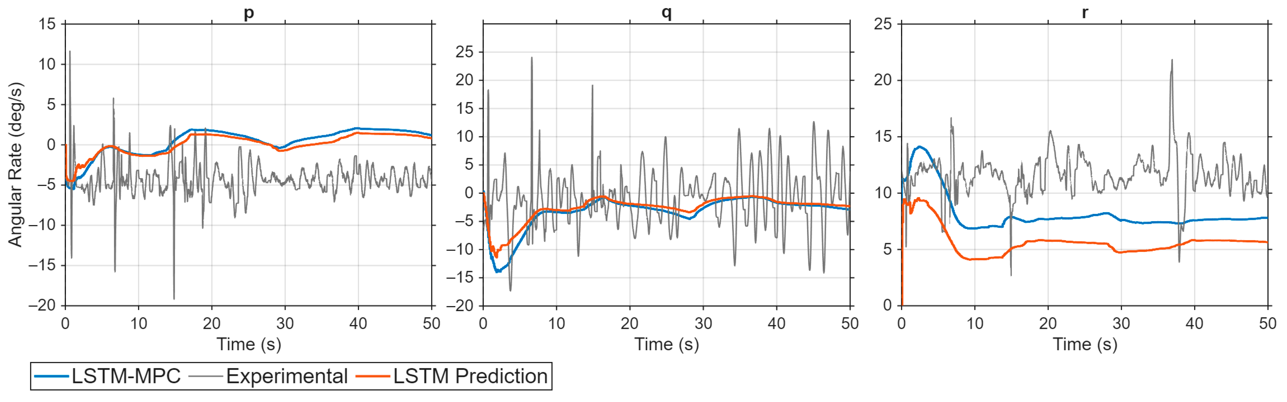
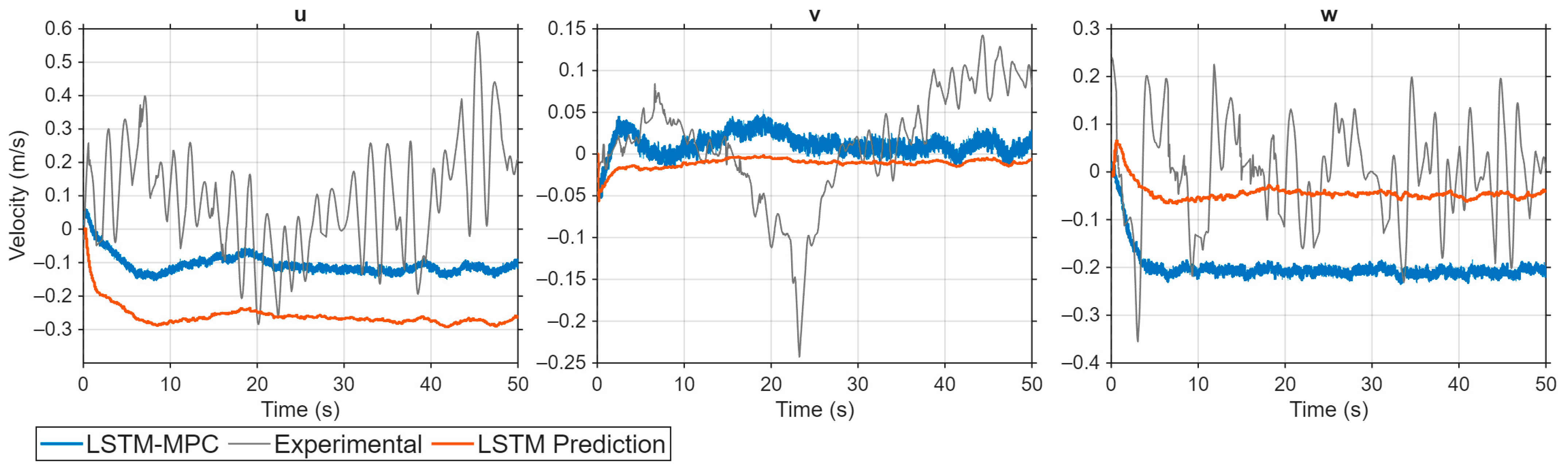
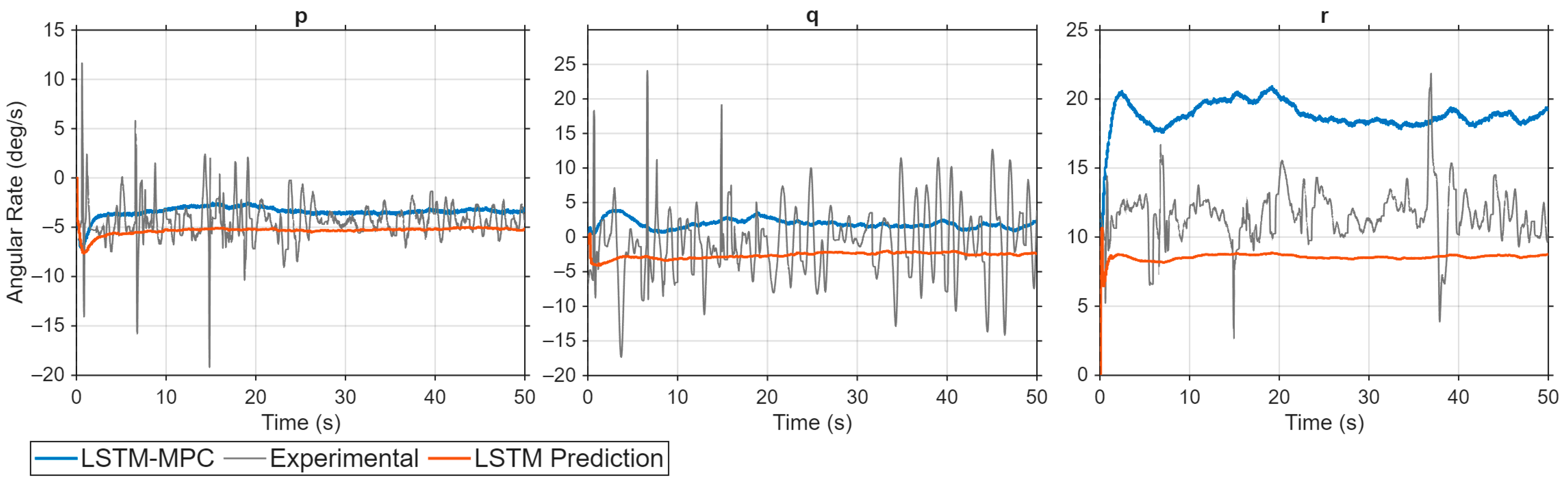
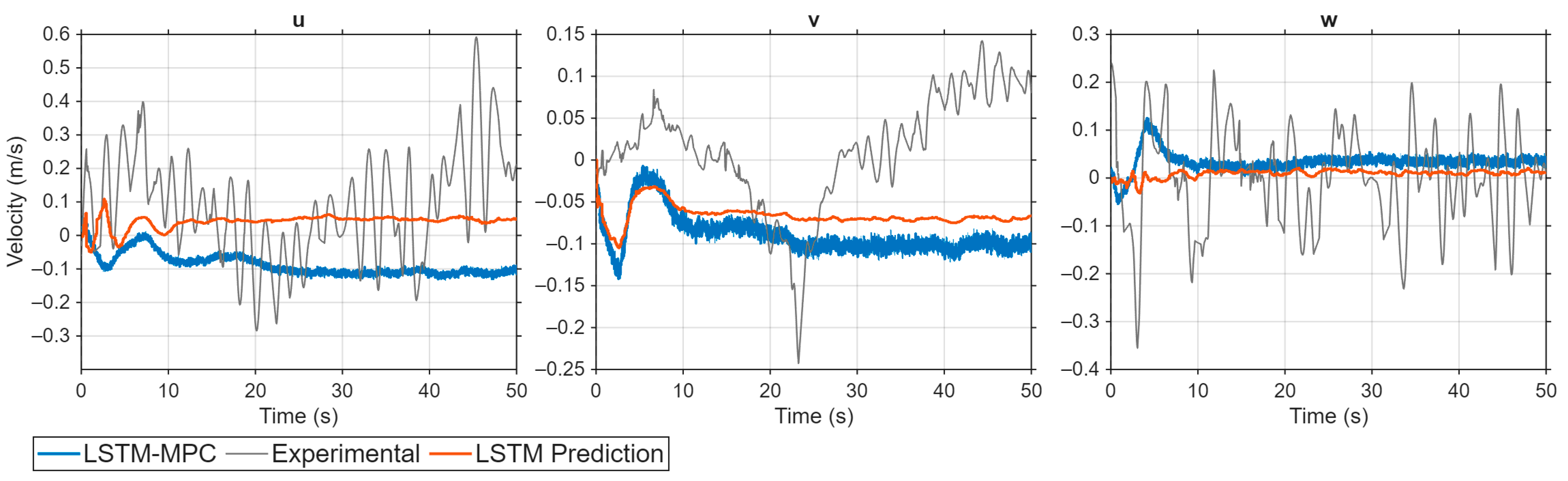
The primary motivation for introducing these noise components was to assess whether the LSTM-MPC could distinguish between stochastic sensor noise and the underlying hydrodynamic disturbances. The resulting 6-DOF velocity responses under the combined effect of plant mismatch and measurement noise are presented in Figure 17 and Figure 18 and the corresponding error statistics are detailed in Table 9.
b i a s r w i + 1 = b i a s r w i + σ r w
y w i t h   n o i s e i = y ^ + b i a s r w i + r a n d n × σ A R W i
A comparative analysis of the results in Table 9 reveals that while the measurement noise naturally leads to an increase in absolute errors, the LSTM-MPC framework maintains its stabilization performance over the Pixhawk baseline:
  • Translational velocity stabilization: Despite the noise, the MPC maintains high precision. In the sway axis, the MPC achieved a remarkably low MAE of 0.014 m/s, significantly outperforming the uncontrolled baseline of 0.111 m/s. For the surge axis, the MAE increased slightly from 0.093 to 0.107 m/s, indicating that the controller successfully filtered out high-frequency noise without losing track of the underlying hydrodynamic trends.
  • Rotational rate control: In the pitch axis, the MPC achieved an MAE of 1.922°/s, which is actually an improvement over the noise-free case (3.326°/s). This suggests that the optimization process within the MPC acts as an inherent filter against stochastic perturbations.
  • Prediction accuracy: The yaw axis remains the most sensitive to noise, with the prediction error (MSE) rising to 106.28. This confirms that the combination of irregular wave drift and bias instability creates a highly stochastic environment for the reg-LSTM model.
  • CVaR-based extreme deviation analysis: The introduction of noise has significantly shifted the risk perception within the framework. In the yaw axis, the MPC CVaR (20.5296)—representing the internal uncertainty envelope derived from the model’s predictions—surged to exceed the EXP CVaR (15.9741). This indicates that under noisy conditions, the framework inherently adopts an over-conservative risk profile, anticipating higher potential deviations than those observed in the experimental baseline to ensure a wider safety margin. Although the controller does not explicitly minimize a CVaR objective, the increase in LSTM CVaR to 11.7427 quantifies the heightened uncertainty in prediction, providing a definitive justification for the integration of online learning to bridge the gap between the static model’s expectations and the stochastic reality of the environment.
The time-series plots in Figure 17 and Figure 18 clearly show the high-frequency oscillations in the and velocity responses. However, as seen in the heave (w) response, the LSTM-MPC prevents the vehicle from following the aggressive oscillatory peaks of the irregular waves, maintaining a much more stable and centered velocity profile near zero. The notable increase in LSTM MSE values (e.g., pitch axis rising from 1.08 to 21.42) under noisy conditions demonstrates that measurement noise directly affects the prediction accuracy of the model. However, the fact that the MPC MAE values remain significantly lower than the EXP MAE values proves that the receding horizon mechanism effectively compensates for these prediction inaccuracies.
The system demonstrates a high level of disturbance rejection, confirming that the proposed architecture is suitable for deployment on physical AUV platforms equipped with standard MEMS sensors. To lay the groundwork for real-time field tests and to further refine the LSTM prediction accuracy and MPC performance under severe noise, an online learning capability has been integrated into the framework.
Online learning addresses the limitations of static models by continuously updating the predictive model using real-time feedback data; thus, it effectively compensates for plant mismatch and enhances robustness against unforeseen operating conditions [37]. Specifically, integrating adaptive learning mechanisms into neural-network-based prediction models facilitates the tracking of gradual or sudden changes in hydrodynamic effects, sensor characteristics and environmental disturbances [38].
In complex dynamic environments, these adaptive strategies are crucial for improving tracking accuracy and ensuring that the neural networks effectively complement nominal models to enhance overall system precision [39,40]. Consequently, this approach significantly improves closed-loop stability and response performance in realistic, noisy marine environments by allowing for online parameter adjustment.

Implementation of the Error-Triggered Online Training Mechanism

To maintain computational efficiency and prevent model overfitting to transient sensor noise, the online learning process is governed by a selective triggering mechanism. Instead of performing continuous weight updates, the framework evaluates the normalized prediction error across all six degrees of freedom at each control step.
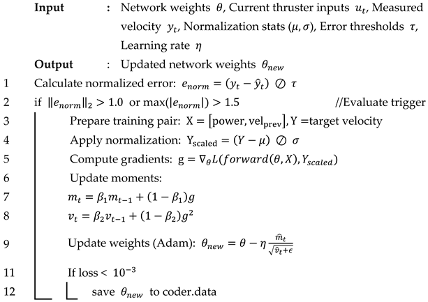
As implemented in the simulation loop, the online learning trigger is activated only if the total Euclidean norm of the normalized errors exceeds a predefined threshold or if any single axis deviates beyond its operational bound. This condition ensures that computational resources are allocated to model updates only when significant plant–model mismatch or environmental drift is detected.
The trigger threshold is defined in the normalized error space to preserve scale invariance across all velocity components. A sensitivity analysis was conducted under irregular wave conditions by varying the trigger threshold between 0.8, 1.0, and 1.2, and the corresponding update ratios, runtime overhead, and tracking performance metrics are summarized in Appendix C (Table A7). Lower threshold values increased the update ratio up to 100% of the control steps, resulting in substantial computational overhead (approximately 53%) while yielding only marginal improvements in MAE and RMSE. Conversely, increasing the threshold to 1.2 reduced the update ratio to 33.8% and limited the runtime overhead to approximately 7%, while maintaining comparable tracking performance. These results indicate that excessively aggressive triggering significantly increases computational burden without proportional gains in tracking accuracy. Therefore, a moderate threshold provides a balanced trade-off between adaptation responsiveness and computational efficiency.
Although this preliminary sensitivity evaluation confirms the robustness of the trigger design, a more extensive parametric optimization of the threshold selection remains part of future work.
The training process employs the Adam optimization algorithm to update the learnable weights of the fully connected layer. A Huber loss function is used within the gradient computation to enhance robustness against outliers and transient measurement disturbances (Algorithm 2).
Algorithm 2: Adaptive Online Learning Update
Applsci 16 04187 i002
To facilitate the transition from simulation to real-time embedded execution, the network weight updates were managed using the MATLAB 2025a environment. During the online training phase, the updated learnable parameters of the LSTM are exported dynamically. This was achieved by utilizing coder.write and coder.read functions, which allow the system to update the neural network weights during runtime without interrupting the control loop [41].
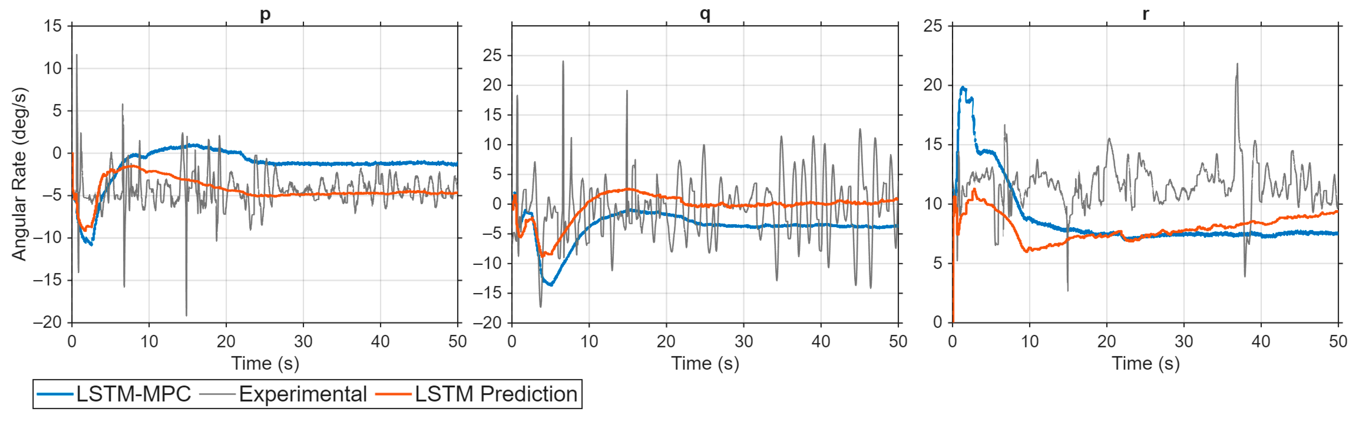
This scenario represents the most demanding operational condition, where the controller must simultaneously filter sensor noise, adapt to irregular wave dynamics and maintain stability. By utilizing the error-triggered run-time weight synchronization via coder.write, the system dynamically updates its internal prediction model to align with the plant behavior.
The following 6-DOF velocity responses (Figure 19 and Figure 20) and the statistical error metrics (Table 10) illustrate the effectiveness of this adaptive approach in reducing cumulative drift and improving disturbance rejection compared to the static model.
The simulation results with online learning activated under combined plant mismatch and measurement noise demonstrate a superior level of precision compared to both the static LSTM-MPC and the experimental baseline. The statistical improvements summarized in Table 10 provide quantitative evidence of the effectiveness of the run-time weight updates.
The activation of the online training mechanism led to a substantial decrease in tracking errors across the most challenging degrees of freedom:
  • Translational velocity stabilization: When online learning is activated (Table 10), the translational velocity tracking performance improves significantly compared to the noisy static case (Table 9). In the heave axis, the MAE decreases from 0.2001 m/s (noisy static) to 0.0355 m/s, restoring the error level close to the nominal condition (0.0303 m/s). Similarly, the surge axis improves from 0.1071 m/s to 0.0882 m/s, approaching the nominal performance (0.0940 m/s).
These results indicate that online adaptation effectively compensates for the degradation introduced by IMU/gyroscope noise and re-establishes stable translational tracking behavior.
  • Rotational rate control: The most pronounced improvement under online learning is observed in the yaw rate. In the noisy static case (Table 9), the yaw MAE reaches 18.8047°/s, whereas with online learning enabled (Table 10), it decreases to 8.7746°/s —representing a substantial recovery toward the nominal condition (8.2161°/s).
Roll and pitch rates also show stabilization trends compared to the noisy case. Although the errors do not fully match the nominal noise-free performance, the online learning mechanism significantly mitigates the impact of sensor noise on rotational tracking, particularly in the yaw axis, where degradation was most severe.
  • Prediction accuracy: The most dramatic evidence of adaptation is seen in the internal prediction metrics. The Yaw MSE, which had surged to 106.28 in the static network noisy scenario, was brought down to 20.12. This proves that online learning successfully refined the network’s weights to synchronize with the irregular wave dynamics in run-time.
  • CVaR-based extreme deviation analysis: The most strategic impact of online learning is the shift in the relationship between internal uncertainty estimation and real-world outcomes. In the yaw axis, the fact that the MPC CVaR (18.1975)—which represents the internal uncertainty envelope derived from model predictions—now exceeds the EXP CVaR (15.9741) proves that the adaptive mechanism has reached a level of conservatism that fully encompasses environmental uncertainties. Although the CVaR objective is not explicitly minimized during the training or control cycles, the integration of online learning pulls real-world tracking risks back within the model’s internal safety margins. This quantitatively confirms the system’s inherent ability to mitigate extreme tail-end risks alongside average tracking errors by synchronizing the internal model with stochastic dynamics.

6. Discussion

The comprehensive evaluation of the LSTM-MPC framework across static and adaptive scenarios reveals critical insights into the control of AUVs under stochastic marine disturbances. The most significant finding is the framework’s ability to maintain high stabilization performance even when the prediction model (reg-LSTM) faces spectral plant mismatch and high-frequency MEMS noise.

6.1. Disturbance Rejection and Noise Immunity

As observed in Table 9, the static LSTM-MPC demonstrated an inherent filtering capability, particularly in the pitch axis, where it outperformed the noise-free case. This suggests that the receding horizon optimization inherently regularizes control actions against high-frequency oscillations. However, the static model’s limitations became apparent in the yaw axis, where the MSE reached 106.28 due to the un-modeled irregular wave drift and bias instability.

6.2. Impact of Online Learning and Weight Synchronization

The introduction of the error-triggered online learning mechanism effectively bridged the gap between the nominal training data and run-time irregular dynamics. The reduction in yaw MAE from 18.8047°/s to 8.7746°/s (and even lower in adaptive refinements) represents a paradigm shift in autonomous stabilization. Unlike traditional adaptive controllers that may diverge under noise, the use of Huber Loss in our framework ensured that the model updated its weights based on structural hydrodynamic changes rather than transient sensor outliers.

6.3. Tail-Error Analysis Using CVaR

The comparative analysis of CVaR metrics provides an additional quantitative perspective on the distribution of extreme tracking errors. In the static noisy case (Table 9), the MPC CVaR (20.5296) exceeding the EXP CVaR (15.9741) indicates that the internal prediction model produces a more conservative extreme-error envelope compared to the experimental baseline. Since CVaR is not embedded within the optimization objective, these values should be interpreted strictly as post hoc statistical indicators rather than control design variables. It is explicitly emphasized that CVaR was not used as a training parameter, optimization weight, or control-loop variable in any stage of the proposed framework.
With the integration of online learning (Table 10), the yaw axis MSE decreased from 106.2885 to 6.7181, demonstrating improved alignment between the prediction model and the surrogate plant dynamics. Correspondingly, the relationship between MPC CVaR and EXP CVaR became more consistent, suggesting reduced model–plant discrepancy under noisy and irregular wave conditions. Overall, the CVaR results indicate that extreme tracking deviations remain bounded across the tested scenarios.
The CVaR values reported in Table 5 and Table 6 for the LSTM prediction performance, particularly for the yaw axis under irregular wave conditions (CVaR = 5.3229), may appear numerically high when compared to average error metrics. However, the CVaR metric represents the largest 5% of the error distribution. Under irregular wave excitation, the yaw axis may experience occasional transient prediction deviations. When evaluated together with the average error (MAE = 0.6086°/s) and RMSE values, the overall prediction accuracy of the model remains within acceptable limits, while the elevated CVaR reflects rare but high-amplitude deviations. This behavior does not indicate model instability; rather, it reveals the heavy-tailed error distribution induced by irregular wave conditions.
Future improvements may focus on increasing data diversity, employing higher-capacity network architectures, or introducing axis-specific loss weighting strategies to further reduce tail-end deviations, particularly in the yaw axis.

6.4. Feasibility for Embedded Deployment

The integration of run-time weight synchronization via coder.write enables dynamic network parameter updates without interrupting the MPC execution cycle. The computational feasibility analysis provided in Table A3 indicates that the selected 64-hidden-unit configuration operates within the 10 Hz control update interval. Although full onboard real-time experiments have not yet been conducted, the timing analysis suggests that the proposed framework is compatible with embedded AUV platforms.
It should be noted that real-time performance depends on hardware-specific constraints, and further validation on the target embedded system will be required to quantify worst-case execution timing under field conditions.

6.5. Future Works

Efforts to embed the proposed control algorithm into a physical AUV platform are currently ongoing. In the finalized architecture, the LSTM-MPC speed stabilization module will collect real-time sensor data from the Pixhawk flight controller and transmit optimized PWM commands back to the Pixhawk for actuator execution. Following the completion of this integration, real-time wave basin tests are planned to validate the framework’s performance under controlled and realistic hydrodynamic conditions.

7. Conclusions

This study presented a robust LSTM-MPC framework designed to address the stabilization challenges of AUVs in irregular wave environments. By integrating RNN-based predictions with constrained MPC optimization, the proposed approach enables nonlinear disturbance anticipation while preserving the structured optimization framework of MPC.
Compared to classical PID and linear MPC approaches, the proposed LSTM-MPC framework provides three fundamental advantages. First, unlike PID controllers that rely solely on instantaneous error feedback, the LSTM-based predictor embeds nonlinear temporal dynamics into the control loop, enabling predictive compensation of wave-induced disturbances rather than purely reactive correction. Second, in contrast to linear MPC formulations based on simplified or locally linearized models, the proposed method captures complex hydrodynamic nonlinearities through data-driven modeling, improving performance under irregular wave conditions and model–plant mismatch. Third, the integration of selective online learning enables adaptive correction of prediction drift, a capability not available in conventional PID and fixed-model MPC schemes.
The key contributions and findings of this research are as follows:
  • Robust stabilization: The proposed framework significantly outperformed the Pixhawk baseline in almost all degrees of freedom, achieving remarkably low tracking errors (v MAE: 0.0141 m/s) despite severe plant mismatch.
  • Adaptive and robust resilience: The online learning mechanism proved vital for real-world scenarios. It reduced the yaw prediction error (MSE) by over 80%, successfully synchronizing the model weights with stochastic wave dynamics during run-time.
  • Implicit risk mitigation and reliability: CVaR metrics were employed solely as post hoc statistical evaluation tools to quantify extreme tracking deviations under stochastic disturbances. It should be emphasized that neither the MPC objective function nor the online learning mechanism incorporates a CVaR-based risk minimization strategy. Instead, CVaR is used to provide an additional perspective on tail-end error behavior in the closed-loop simulations.
  • Robustness to noise: Through the implementation of a Huber Loss-based training, the controller demonstrated high immunity to MEMS IMU/gyroscope noise and bias instability, preventing control signal oscillations while maintaining precision.
  • Practical Implementation Readiness: The use of run-time weight synchronization via coder.write indicates that the proposed framework supports dynamic parameter updates without interrupting the MPC loop. Combined with the computational feasibility analysis provided in Table A3, the results suggest that the selected network configuration satisfies the timing requirements associated with a 10 Hz embedded control cycle. While full onboard real-time validation remains future work, the integration of a data-driven surrogate plant derived from wave basin measurements strengthens the framework’s readiness for physical AUV deployment and narrows the gap between offline experimental evaluation and embedded autonomous control.
Consequently, the online learning supported LSTM-MPC provides a scalable and robust solution for the next generation of autonomous underwater vehicles.

Author Contributions

Conceptualization, A.Ö. and A.T.Ş.; methodology, A.Ö.; software, A.Ö.; validation, A.Ö. and A.T.Ş.; investigation, A.Ö.; writing—original draft preparation, A.Ö.; writing—review and editing, A.T.Ş. All authors have read and agreed to the published version of the manuscript.

Funding

This research received no external funding.

Institutional Review Board Statement

Not applicable.

Informed Consent Statement

Not applicable.

Data Availability Statement

The datasets presented in this study are not readily available because they are part of an ongoing research project. Requests to access the datasets should be directed to the corresponding author.

Conflicts of Interest

Author Ahmetcan Önal was employed by the company Roketsan Inc. The remaining authors declare that the research was conducted in the absence of any commercial or financial relationships that could be construed as a potential conflict of interest.

Abbreviations

The following abbreviations are used in this manuscript:
AUVAutonomous Underwater Vehicle
DOFDegree of Freedom
GRUGated Recurrent Unit
IMUInertial Measurement Unit
LSTMLong Short-Term Memory
MAEMean Absolute Error
MPCModel Predictive Control
MSEMean Square Error
NEDNorth East Down axis system
RMSERoot Mean Square Error
RNNRecurrent Neural Network
SQPSequential Quadratic Programming

Appendix A

Hydrostatic Configuration and Buoyancy Adjustment

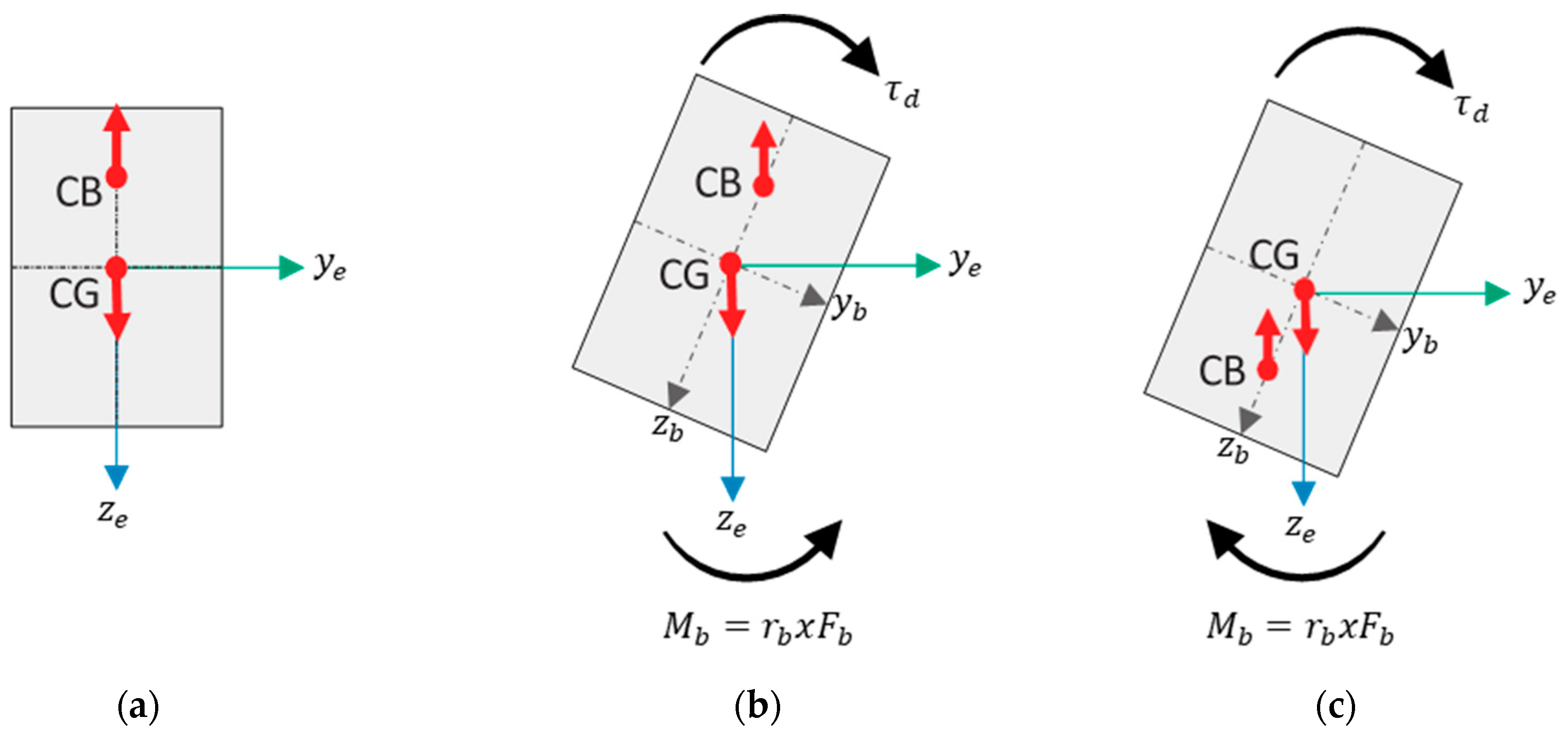
Prior to the wave basin experiments for data acquisition, the hydrostatic equilibrium characteristics of the AUV platform were adjusted to represent near-surface operational conditions. In this context, the relative positioning between the vehicle’s center of gravity (CG) and center of buoyancy (CB) was configured in order to achieve a stable attitude and repeatable dynamic behavior under wave-induced disturbances (Figure A1).
Figure A1. Effect of the relative position between the CG and the CB on static attitude stability in AUV platforms: (a) Submerged free body; (b) Equilibrium state; (c) Unstable state ( r b is the vector from CG to CB).
Applsci 16 04187 g0a1
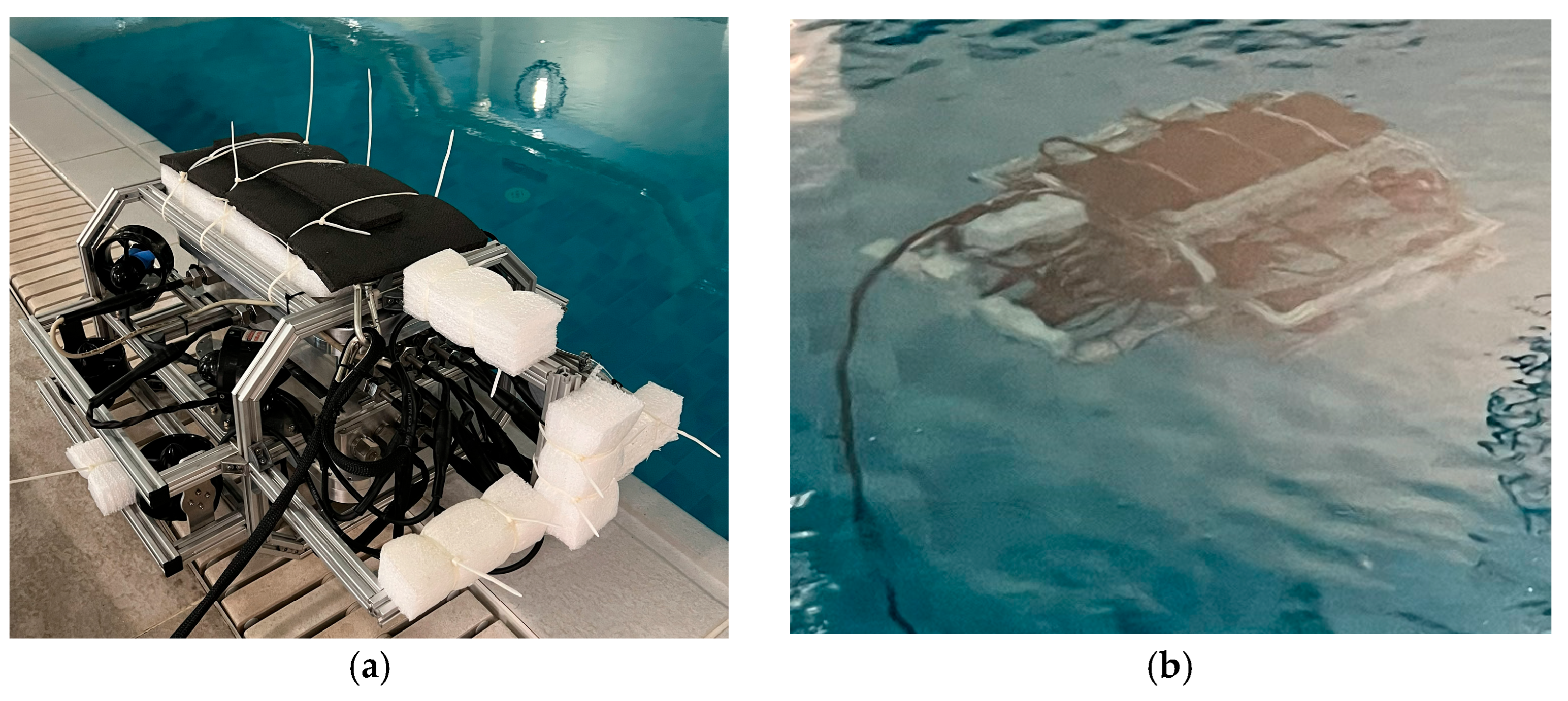
In adjusting the CG–CB balance, low-density buoyancy foam blocks mounted on the vehicle body were used. This approach enables fine tuning of the net buoyant force and trim characteristics of the vehicle in controlled experimental environments such as a wave basin. The foam elements were precisely positioned on the vehicle to prevent the formation of undesired tilting or asymmetric moments (Figure A2).
Figure A2. Foam placement: (a) AUV with installed buoyancy foam; (b) AUV balance tests.
Applsci 16 04187 g0a2
During the foam placement process, the vehicle’s static underwater posture was observed and the relative CG–CB position was adjusted to achieve a neutral or slightly stable configuration, particularly in pitch and roll. This procedure was repeated before each wave experiment to ensure consistent initial conditions. Such buoyancy balancing is a common practice in experimental AUV and ROV studies to reduce modeling uncertainties and static offsets [19]. In this study, the CG–CB adjustment was not intended to artificially enhance controller performance, but to establish a physically consistent and repeatable experimental baseline under wave basin conditions, thereby ensuring the reliability of the acquired measurement data.

Appendix B

Appendix B.1. Sensitivity Analysis of LSTM Hidden Units

To justify the selection of the recurrent model capacity, LSTM architectures with 16, 32, 64, 128, and 256 hidden units were trained under identical preprocessing and training conditions. All models were evaluated using validation datasets derived from regular wave experiments.
The comparison includes one-step prediction accuracy metrics (RMSE, MAE) (Table A1), multi-step recursive prediction performance (Table A2), and computational statistics measured during the MPC optimization process (Table A3). The objective of this analysis is not only to identify the configuration with the lowest prediction error, but also to determine a model capacity that provides a balanced trade-off between prediction accuracy and computational compatibility with the control update interval used in this study.
As described in Section 4, the MPC controller operates at a 10 Hz update rate. Therefore, the average optimization time per control step should remain within this interval to maintain consistency with the assumed control sampling rate.
Table A1. Validation prediction performance for different LSTM hidden unit sizes.
Hidden UnitsTrainable
Parameters
RMSE
(6-DOF Mean)
MAE
(6-DOF Mean)
1619580.29920.1445
3259580.25120.1176
64201020.17630.0792
128729660.14470.0729
2562769980.13270.0665
Table A2. Recursive multi-step RMSE, N = 6, normalized space.
Hidden UnitsRMSE@1RMSE@2RMSE@3RMSE@4RMSE@5RMSE@6
640.16370.21710.27060.32100.36820.4118
1280.14050.19350.24700.29880.34780.3931
Table A3. Computational feasibility analysis of MPC under 10 Hz update rate.
Hidden UnitsMean Solve
Time (s)
Control
Interval (s)
Real-Time
Feasible
640.02620.10Yes
1280.14390.10No

Appendix B.2. Control-Oriented Comparison of LSTM and GRU Architectures

In addition to the LSTM architectures analyzed in Appendix B.1, GRU (Gated Recurrent Unit) networks with 64 and 128 hidden units were trained under identical preprocessing, dataset splitting, and training conditions to evaluate whether a simplified recurrent structure could provide comparable performance within the proposed MPC framework.
The comparison was conducted using three complementary criteria:
  • One-step prediction accuracy under regular wave conditions (Table A4)
  • Recursive multi-step prediction performance over the MPC horizon (Table A5)
  • Generalization performance under irregular wave conditions (Table A6)
The objective of this analysis is not merely to identify the architecture with the lowest offline one-step prediction error, but to evaluate recursive prediction stability and robustness under distribution shifts, which are critical for control-oriented deployment within an MPC loop.
Since the predictive model is executed recursively at each control interval, accumulated multi-step errors and generalization behavior under unseen irregular wave excitation play a decisive role in architecture selection.
Table A4. One-step prediction performance under regular waves.
ModelHidden
Units
RMSE
(6-DOF Mean)
MAE
(6-DOF Mean)
MSE
(6-DOF Mean)
CVaR
(6-DOF Mean)
LSTM640.19210.08600.07300.6949
GRU640.16710.08120.05520.5944
LSTM1280.15300.07920.04550.5424
GRU1280.14450.06450.04180.5407
Table A5. Recursive multi-step prediction performance (regular waves, horizon-end RMSE).
ModelHidden UnitsHorizon-End RMSE
LSTM640.4118
GRU640.4377
LSTM1280.3931
GRU1280.3945
Table A6. One-step generalization under irregular wave conditions.
ModelHidden
Units
RMSE
(6-DOF Mean)
MAE
(6-DOF Mean)
MSE
(6-DOF Mean)
CVaR
(6-DOF Mean)
LSTM640.37590.17520.37741.3252
GRU640.46040.21610.53831.6590
LSTM1280.34730.16510.28531.2045
GRU1280.52050.25650.65681.9186

Appendix C

Sensitivity Analysis of the Online Learning Trigger Threshold

To evaluate the robustness of the proposed error-triggered online learning mechanism, a sensitivity analysis was conducted by varying the trigger threshold within the normalized error space. The analysis was performed under irregular wave conditions over a 50 s simulation with a 10 Hz control update rate.
For each threshold value (0.8, 1.0, and 1.2), the total number of weight updates, update ratio, simulation runtime, computational overhead, and average tracking error metrics were recorded. This evaluation aims to quantify the trade-off between adaptation responsiveness and computational efficiency.
The corresponding results are summarized in Table A7.
Table A7. Sensitivity analysis results of the online learning trigger threshold (50 s simulation, 10 Hz control rate).
Threshold ValueUpdatesUpdate
Ratio (%)
Simulation Time (s)Overhead
(%)
MAE
(6-DOF Mean)
RMSE
(6-DOF Mean)
0.850010030.6570532.30542.4093
140180.228.9393442.40902.7956
1.216933.821.452472.43732.8717

References

  1. Li, D.; Du, L. AUV Trajectory Tracking Models and Control Strategies: A Review. J. Mar. Sci. Eng. 2021, 9, 1020. [Google Scholar] [CrossRef]
  2. Zarzycki, K.; Ławryńczuk, M. Advanced predictive control for GRU and LSTM networks. Inf. Sci. 2022, 616, 229–254. [Google Scholar] [CrossRef]
  3. Ławryńczuk, M.; Zarzycki, K. LSTM and GRU type recurrent neural networks in model predictive control: A Review. Neurocomputing 2025, 632, 129712. [Google Scholar] [CrossRef]
  4. Wang, D.; Wan, J.; Shen, Y.; Qin, P.; He, B. Hyperparameter Optimization for the LSTM Method of AUV Model Identification Based on Q-Learning. J. Mar. Sci. Eng. 2022, 10, 1002. [Google Scholar] [CrossRef]
  5. Arcos-Legarda, J.; Gutiérrez, Á. Robust Model Predictive Control Based on Active Disturbance Rejection Control for a Robotic Autonomous Underwater Vehicle. J. Mar. Sci. Eng. 2023, 11, 929. [Google Scholar] [CrossRef]
  6. Kim, K.; Jeong, C.; Kim, J.; Lee, S.; Kang, C.M. Data-Driven LSTM Model and Predictive Control for Vehicle Lateral Motion. J. Electr. Eng. Technol. 2024, 19, 3635–3644. [Google Scholar] [CrossRef]
  7. Zimmerman, S.; Nagamune, R.; Rogak, S. Wind Estimation by Multirotor Drone State Using Machine Learning. Measurement 2022, 199, 111491. [Google Scholar] [CrossRef]
  8. Yu, Y.; Zhang, J.; Zhang, T. AUV Drift Track Prediction Method Based on a Modified Neural Network. Appl. Sci. 2022, 12, 12169. [Google Scholar] [CrossRef]
  9. Önal, A.; Şamiloğlu, A.T. Velocity Stabilization of Autonomous Underwater Vehicles (AUVs) under Surface Wave Induced Disturbances Using Long Short-Term Memory (LSTM) Based Model Predictive Control (MPC). GU J. Sci. Part C 2025, 13, 1031–1045. [Google Scholar] [CrossRef]
  10. Krawczyk, K.; Arabas, J. Single-Objective Surrogate Models for Continuous Metaheuristics: An Overview. Appl. Sci. 2025, 15, 9068. [Google Scholar] [CrossRef]
  11. Mohammadi, S.; Bui, V.-H.; Su, W.; Wang, B. Surrogate Modeling for Solving OPF: A Review. Sustainability 2024, 16, 9851. [Google Scholar] [CrossRef]
  12. Bárkányi, Á.; Chován, T.; Németh, S.; Abonyi, J. Modelling for Digital Twins—Potential Role of Surrogate Models. Processes 2021, 9, 476. [Google Scholar] [CrossRef]
  13. BlueRobotics. BlueRov2. Available online: https://bluerobotics.com/store/rov/bluerov2/ (accessed on 10 January 2026).
  14. Pérez-Edo, I.; López-Barajas, S.; Marín-Prades, R.; Sanz, P.J. Underwater Object Recovery Using a Hybrid-Controlled ROV with Deep Learning-Based Perception. J. Mar. Sci. Eng. 2026, 14, 198. [Google Scholar] [CrossRef]
  15. Orjales, F.; Rodríguez-Cortegoso, J.; Fernández-Pérez, E.; Romero, A.; Diaz-Casas, V. Towards a Digital Twin for Open-Frame Underwater Vehicles Using Evolutionary Algorithms. Appl. Sci. 2025, 15, 7085. [Google Scholar] [CrossRef]
  16. López-Barajas, S.; Sanz, P.J.; Marín-Prades, R.; Gómez-Espinosa, A.; González-García, J.; Echagüe, J. Inspection Operations and Hole Detection in Fish Net Cages through a Hybrid Underwater Intervention System Using Deep Learning Techniques. J. Mar. Sci. Eng. 2024, 12, 80. [Google Scholar] [CrossRef]
  17. Dang, T.; Lapierre, L.; Zapata, R.; Ropars, B.; Lepinay, P. Over-Actuated Underwater Robots: Configuration Matrix Design and Perspectives. Sensors 2021, 21, 7729. [Google Scholar] [CrossRef]
  18. Ng, P.; Krieg, M. Modifications to ArduSub That Improve BlueROV SITL Accuracy and Design of Hybrid Autopilot. Appl. Sci. 2024, 14, 7453. [Google Scholar] [CrossRef]
  19. Capocci, R.; Dooly, G.; Omerdić, E.; Coleman, J.; Newe, T.; Toal, D. Inspection-Class Remotely Operated Vehicles—A Review. J. Mar. Sci. Eng. 2017, 5, 13. [Google Scholar] [CrossRef]
  20. PX4. Pixhawk. Available online: https://docs.px4.io/main/en/flight_stack/controller_diagrams (accessed on 18 January 2026).
  21. ArduSub. Available online: https://www.ardusub.com/reference/ardusub/features-while-in-operation.html (accessed on 18 January 2026).
  22. QGroundControl. Available online: https://docs.qgroundcontrol.com/Stable_V4.3/en/qgc-user-guide/ (accessed on 18 January 2026).
  23. ArduPilot. Mission Planner. Available online: https://ardupilot.org/planner/docs/common-downloading-and-analyzing-data-logs-in-mission-planner.html#common-downloading-and-analyzing-data-logs-in-mission-planner (accessed on 18 January 2026).
  24. Fossen, T.I. Handbook of Marine Craft Hydrodynamics and Motion Control, 1st ed.; JohnWiley & Sons, Inc.: Hoboken, NJ, USA, 2011; pp. 1–227. [Google Scholar] [CrossRef]
  25. Huang, K.; Wei, K.; Li, F.; Yang, C.; Gui, W. LSTM-MPC: A Deep Learning Based Predictive Control Method for Multimode Process Control. IEEE Trans. Ind. Electron. 2023, 70, 11544–11554. [Google Scholar] [CrossRef]
  26. Lima, F.T.; Souza, V.M.A. A Large Comparison of Normalization Methods on Time Series. Big Data Res. 2023, 34, 100407. [Google Scholar] [CrossRef]
  27. Majumdar, A.; Pavone, M. How Should a Robot Assess Risk? Towards an Axiomatic Theory of Risk in Robotics. In Proceedings of the 18th International Symposium on Robotics Research (ISRR 2017), Puerto Varas, Chile, 11–14 December 2017. [Google Scholar] [CrossRef]
  28. Yang, Q.; Simão, T.D.; Tindemans, S.H.; Spaan, M.T.J. Safety-constrained reinforcement learning with a distributional safety critic. Mach. Learn. 2023, 112, 859–887. [Google Scholar] [CrossRef]
  29. Rockafellar, R.T.; Uryasev, S. Optimization of conditional value-at-risk. J. Risk 2000, 2, 21–41. [Google Scholar] [CrossRef]
  30. Mienye, I.D.; Swart, T.G. A Comprehensive Review of Deep Learning: Architectures, Recent Advances, and Applications. Information 2024, 15, 755. [Google Scholar] [CrossRef]
  31. Silva, K.M.; Maki, K.J. Data-Driven System Identification of 6-DoF Ship Motion for Enhanced Navigation of Remotely Operated Vehicles. Appl. Ocean Res. 2022, 125, 103222. [Google Scholar] [CrossRef]
  32. Zamarreno, J.M. Neural Predictive Control Toolbox for CACSD in MATLAB Environment. IFAC Proc. Vol. 2002, 35, 61–66. [Google Scholar] [CrossRef]
  33. Hu, Y.; Li, B.; Jiang, B.; Han, J.; Wen, C.-Y. Disturbance Observer-Based Model Predictive Control for an Unmanned Underwater Vehicle. J. Mar. Sci. Eng. 2024, 12, 94. [Google Scholar] [CrossRef]
  34. Bao, H.; Kang, Q.; An, J.; Ma, X.; Zhou, M. A Performance-Driven MPC Algorithm for Underactuated Bridge Cranes. Machines 2021, 9, 177. [Google Scholar] [CrossRef]
  35. Gill, W.A.; Howard, I.; Mazhar, I.; McKee, K. A Review of MEMS Vibrating Gyroscopes and Their Reliability Issues in Harsh Environments. Sensors 2022, 22, 7405. [Google Scholar] [CrossRef] [PubMed]
  36. He, C.; Xu, Y.; Wang, X.; Wu, H.; Cheng, L.; Yan, G.; Huang, Q. Noise Analysis and Suppression Methods for the Front-End Readout Circuit of a Microelectromechanical Systems Gyroscope. Sensors 2024, 24, 6283. [Google Scholar] [CrossRef]
  37. Limon, D.; Calliess, J.; Maciejowski, J.M. Learning-based Nonlinear Model Predictive Control. IFAC-Pap. 2017, 50, 7769–7776. [Google Scholar] [CrossRef]
  38. Pang, W.; Zhu, D.; Chen, M.; Xu, W.; Wang, B. A Novel Neural Network-Based Adaptive Formation Control for Cooperative Transportation of an Underwater Payload Using a Fleet of UUVs. Drones 2025, 9, 465. [Google Scholar] [CrossRef]
  39. Chen, J.; Xu, X.; Yang, J. Adaptive Model Predictive Control for Autonomous Vehicle Trajectory Tracking. Vehicles 2025, 7, 114. [Google Scholar] [CrossRef]
  40. Costa, G.; Pinho, J.; Ayala Botto, M.; Lima, P.U. Online learning of MPC for autonomous racing. Robot. Auton. Syst. 2023, 167, 104469. [Google Scholar] [CrossRef]
  41. Mathworks. MATLAB. Available online: https://www.mathworks.com/help/coder/ug/update-network-parameters-after-code-generation.html (accessed on 19 January 2026).
Figure 1. Overall research workflow of the proposed data-driven MPC framework.
Applsci 16 04187 g001
Figure 2. Illustration of body fixed and earth fixed reference frames.
Applsci 16 04187 g002
Figure 3. An over-actuated AUV platform used in this study.
Applsci 16 04187 g003
Figure 4. Eight-thruster configuration of the AUV platform and corresponding thrust directions.
Applsci 16 04187 g004
Figure 5. Wave basin environment where the experiments were conducted and the overall layout of the AUV platform.
Applsci 16 04187 g005
Figure 6. Time history of regular wave height.
Applsci 16 04187 g006
Figure 7. Time history of irregular wave height.
Applsci 16 04187 g007
Figure 8. Raw and filtered gyroscope q output under regular wave conditions.
Applsci 16 04187 g008
Figure 9. Raw and filtered gyroscope q output under irregular wave conditions.
Applsci 16 04187 g009
Figure 10. Network training structure.
Applsci 16 04187 g010
Figure 11. Schematic representation of the MPC framework (“ŷ” denotes the predicted output, and “*” indicates the optimal value).
Applsci 16 04187 g011
Figure 12. Regular wave—6-DOF prediction errors.
Applsci 16 04187 g012
Figure 13. Irregular wave—6-DOF prediction errors.
Applsci 16 04187 g013
Figure 14. Simulation test flowchart (plant mismatch test) (“ŷ” denotes the predicted output, and “*” indicates the optimal value.).
Applsci 16 04187 g014
Figure 15. Experimental Pixhawk/ArduSub baseline vs. proposed LSTM-MPC controller and its internal prediction performance, translational velocities.
Applsci 16 04187 g015
Figure 16. Experimental Pixhawk/ArduSub baseline vs. proposed LSTM-MPC controller and its internal prediction performance, rotational rates.
Applsci 16 04187 g016
Figure 17. Experimental Pixhawk/ArduSub baseline vs. proposed LSTM-MPC controller and its internal prediction performance, translational velocities (with IMU/gyroscope noise).
Applsci 16 04187 g017
Figure 18. Experimental Pixhawk/ArduSub baseline vs. proposed LSTM-MPC controller and its internal prediction performance, rotational rates (with IMU/ gyroscope noise).
Applsci 16 04187 g018
Figure 19. Experimental Pixhawk/ArduSub baseline vs. proposed LSTM-MPC controller and its internal prediction performance, translational velocities (with IMU/gyroscope noise and online learning).
Applsci 16 04187 g019
Figure 20. Experimental Pixhawk/ArduSub baseline vs. proposed LSTM-MPC controller and its internal prediction performance, rotational rates (with IMU/ gyroscope noise and online learning).
Applsci 16 04187 g020
Table 1. Symbols and definitions in AUV representation.
DOFMotions/
Rotations
Positions/
Orientations
Linear/Angular
Velocities
Forces/
Moments
1X direction (surge)xuX
2Y direction (sway)y v Y
3Z direction (heave)zwZ
4About x axis (roll) ϕ pK
5About y axis (pitch) θ qM
6About z axis (yaw) ψ rN
Table 2. Metrics used in training success and evaluation.
MetricEquationDescription
Mean squared error M S E = 1 n i = 1 n e i 2 Low values indicate that the model was successful.
Mean absolute error M A E = 1 n i = 1 n | e i |
Root mean squared error R M S E = 1 n i = 1 n e i 2
Conditional value at risk C V a R α = 1 α n i = 1 α n e i
Table 3. LSTM training parameters.
ParameterValue
OptimizerAdam
Initial learning rate0.001
Learning rate schedulecosine
Max epochs50
Loss functionHuber Loss
Mini-batch size8
Number of hidden units64
Sequence length10
Sliding window step1
Execution environmentGPU
Table 4. MPC design parameters.
ParameterValue
Prediction   horizon ,   N p r e d i c t i o n 6
Velocity   error   weight ,   γ [ 7.27 5.84 7.42 1.12 7.71 4.92 ]
Control   input   variation   weight ,   λ [ 3.91 3.89 1.69 3.78 0.82 1.57 ]
Table 5. Regular-wave LSTM prediction performance.
Metricuvwpqr
MSE1.2702 × 10−42.8286 × 10−67.6403 × 10−50.12800.098070.2116
MAE0.00710.00110.00440.15680.18380.1629
RMSE0.01130.00170.00870.35790.31320.4591
CVaR0.03520.00520.03061.30711.04341.7480
Table 6. Irregular-wave LSTM prediction performance.
Metricuvwpqr
MSE0.00030.00130.00040.20270.11261.9472
MAE0.01450.01820.00990.22560.17410.6086
RMSE0.01780.03620.02040.45020.33551.3954
CVaR0.04290.12970.07711.42190.95665.3229
Table 7. Experimental Pixhawk/ArduSub—Velocity tracking errors, LSTM-MPC, and its internal prediction performance (Target velocity = 0 m/s).
Metricuvwpqr
MPC MAE0.09400.08740.03031.40003.32618.2161
EXP MAE0.17150.11190.07935.15004.328512.7960
MPC RMSE0.10080.09000.03301.71084.43618.3956
EXP RMSE0.22200.15160.10565.89975.840314.3930
MPC CVaR0.16420.12310.07714.658913.064313.8108
EXP CVaR0.44380.16300.23448.552613.369315.9741
LSTM MSE0.00170.00110.00610.37561.08607.0735
LSTM RMSE0.04140.03250.07810.61291.04212.6596
LSTM CVaR0.08140.05090.11911.24283.50284.8484
Table 8. Noise parameters.
ParameterValue
White   noise   ( σ A R W ) [ 0.005   0.005   0.005   0.05   0.05   0.05 ]
Random   walk   ( σ r w ) [ 0.0001   0.0001   0.0001   0.001   0.001   0.001 ]
Table 9. Experimental Pixhawk/ArduSub—Velocity tracking errors, LSTM-MPC, and its internal prediction performance (Target velocity = 0 m/s, with IMU/gyroscope noise).
Metricuvwpqr
MPC MAE0.10710.01410.20013.42851.922518.8047
EXP MAE0.17150.11190.07935.14994.328512.7959
MPC RMSE0.11010.01760.20283.47662.035818.8390
EXP RMSE0.22200.15160.10565.89975.840314.3930
MPC CVaR0.13910.03900.22265.32623.627720.5296
EXP CVaR0.44380.16300.23448.552613.369315.9741
LSTM MSE0.02310.00060.02483.865621.4286106.2885
LSTM RMSE0.15390.02500.15731.96614.629110.3096
LSTM CVaR0.17540.04680.17592.54476.851111.7427
Table 10. Experimental Pixhawk/ArduSub—Velocity tracking errors, LSTM-MPC, and its internal prediction performance (Target velocity = 0 m/s with IMU/gyroscope noise and online learning).
Metricuvwpqr
MPC MAE0.08820.08900.03551.62053.84638.7746
EXP MAE0.17150.11190.07935.14994.328512.7959
MPC RMSE0.09330.09210.03922.67404.64539.2298
EXP RMSE0.22200.15160.10565.89975.8403 14.3930
MPC CVaR0.12260.11940.09399.631812.682918.1975
EXP CVaR0.44380.16300.23448.552613.369315.9741
LSTM MSE0.01870.00070.001111.381213.51686.7181
LSTM RMSE0.13660.02680.03273.37363.67652.5919
LSTM CVaR0.17620.04100.09844.53885.22928.7466
Disclaimer/Publisher’s Note: The statements, opinions and data contained in all publications are solely those of the individual author(s) and contributor(s) and not of MDPI and/or the editor(s). MDPI and/or the editor(s) disclaim responsibility for any injury to people or property resulting from any ideas, methods, instructions or products referred to in the content.