Gradient vs. Non-Gradient-Based Model Free Control Algorithms: Analysis and Applications to Nonlinear Systems

Abstract

Against the background of the development of control systems, Data Driven Control (DDC) methods are becoming more and more popular, given the system’s independence from physical models and the possibility of quickly tuning the controller. The usefulness of such tuning algorithms increases with the complexity of the plants. Nonlinear models are the main class of processes for which such laws are amenable. According to the literature, a class of DDC methods exist that perform online estimation of plant behavior with an unknown structure, which is generically called Model Free. This title is assumed by two types of algorithms, which contain it in the name. One is the gradient-based algorithm, Model Free Adaptive Control, defined by Hou, which uses the concept of dynamic linearization through pseudo partial derivatives (PPD) and pseudo gradient (PG). The other is a non-gradient based algorithm, Model Free Control, defined by Fliess and Join, which uses the concept of the ultralocal model and intelligent PID controllers (iPID). For the gradient-based methods, in the compact form of dynamic linearization (CFDL), i.e., partial form dynamic linearization (PFDL), two algorithms are proposed to determine the initial value of the time-varying parameters PPD and PG from the dynamic performance perspective as they offer the best responses. The CFDL and PFDL variants of the MFAC control law, which have parameters that result from the application of the proposed algorithms, are compared with iP and iPD controllers on nonlinear control systems.

1. Introduction

Data-Driven Control (DDC) algorithms have emerged as a powerful alternative to traditional Model-Based Control (MBC) techniques, particularly for systems characterized by nonlinearities, modeling challenges, or inaccessible models. Unlike MBC, which relies on mathematical models, DDC techniques derive their flexibility from their reliance solely on data acquired directly from the control system. By leveraging this data, DDC algorithms dynamically assess the behavior of the controlled process to achieve the desired objectives. The foundational work in this field includes the comprehensive survey by Hou [1], with an updated version presented in [2]. These surveys categorize DDC algorithms based on how data is processed (online or offline), the structure of the algorithm (fixed or unknown), and whether gradient calculations are employed during the control process. Gradient-based methods include Iterative Feedback Tuning (IFT) [3], Iterative Learning Control (ILC) [4], Noniterative Data-Driven Model Reference Control [5], Virtual Reference Feedback Tuning (VRFT) [6], and Model-Free Adaptive Control (MFAC) [7]. Non-gradient methods, on the other hand, encompass Model-Free Control (MFC) [8], Correlation-Based Tuning (CbT) [9], and Unfalsification with Analytic Update [10].

Model-Free methods, which rely exclusively on real-time data from the system, are primarily represented by two approaches: MFAC, introduced by Hou [7], and MFC, developed by Fliess and Join [8]. While both methods share some structural similarities, they differ fundamentally in their underlying principles. MFAC employs dynamic linearization and operates as a gradient-based method, whereas MFC utilizes an ultralocal model and is non-gradient-based. This paper seeks to clarify the distinctions between these two approaches and provide a detailed analysis of their application to nonlinear systems. The adaptive variant introduced by Hou in [7] dynamically linearizes the plant using process data, with its complexity varying based on the volume of data utilized. This method has been successfully applied in diverse domains, including unmanned surface vessels in [11], absorption refrigeration systems [12], flying robots [13], parafoil systems [14], multivehicle systems with constraints [15] and quadrotor formations [16]. Beyond its standard implementation, MFAC has been integrated with other control techniques such as Iterative Feedback Tuning (IFT) [17], Predictive Control (PC) [18], Sliding Mode Control (SMC) [19,20], Iterative Learning Concept (ILC) [21], Fault Tolerant Control (FTC) [22], Virtual Reference Feedback Tuning (VFRT) [23] or Error Minimized Regularized Online Sequential Extreme Learning Machine [24]. The method is well-established, with [7] providing stability analyses for all MFAC variants.

On the other hand, MFC has been applied in areas such as lateral vehicle control [25], ramp metering [26], variable-speed wind turbines [27], quadrotors used for acrobatic flight [28], machine tools [29], and non-minimum phase systems and switched systems [30]. Also, the MFC approach can be used together with other control techniques to be improved, such as in the case of SMC [31], VRFT [32] or IFT [33], to enhance its performance. While MFC is relatively newer compared to MFAC, ongoing research, including [34,35], is addressing its theoretical foundations, particularly in stability analysis.

This paper conducts a comparative analysis of gradient-based (MFAC) and non-gradient-based (MFC) Model-Free methods. MFAC employs dynamic linearization techniques, such as the Compact Form Dynamic Linearization (CFDL) and Partial Form Dynamic Linearization (PFDL), which utilize pseudo partial derivatives (PPD) and pseudo gradients (PG), respectively. To optimize performance, two algorithms are introduced to determine the initial values of PPD and PG, addressing the influence of these parameters on system dynamics, as highlighted in [36,37]. These algorithms aim to minimize control errors and enhance the performance of CFDL and PFDL-based MFAC controllers across various applications. MFC, on the other hand, relies on intelligent PID (iPID) laws, which mimic classical PID behavior but operate without a plant model, using only system data. The iP and iPID algorithms, as described in [8], exhibit behavior akin to PI and PID controllers. Given the suitability of DDC methods for nonlinear systems, this paper applies the proposed algorithms to three such systems: a BLDC motor with nonlinear control elements, a non-minimum phase nonlinear system, and a nonlinear system with time-varying parameters. The analysis aims to evaluate the effectiveness of gradient and non-gradient approaches in these contexts.

Since DDC-type approaches are suitable for nonlinear systems, this paper proposes the application of the algorithms for obtaining the initial values for CFDL and PFDL, respectively the analysis between the gradient and non-gradient based methods, using three such systems. The first is represented by a BLDC motor, which has a control loop with nonlinear elements, the second is represented by a non-minimum phase nonlinear system, and the third is a nonlinear system with a time-varying parameter.

The main contributions of this paper are as follows.

• Determining the initial value of PPD for the MFAC-CFDL law by obtaining the starting value for the time-varying parameter used in the control law equation.
• Determining the initial value of PG for the MFAC-PFDL law by obtaining the starting values for the time-varying parameter used in the control law equation.
• Testing and validation of algorithms for initial values of time-varying parameters in relation to preliminary laws that provide stable responses of control systems
• Comparative analysis of the performance of systems controlled by gradient and non-gradient based methods applied to nonlinear systems.

The structure of the paper comprises a presentation of the two Model Free algorithms which are described in Section 2, followed by the presentation of the nonlinear systems considered to be controlled, in Section 3. In Section 4, the algorithms for determining the optimized values for the PPD and PG are presented, with the results obtained by applying them to the plants mentioned in Section 3. In the same section, the comparative results of the control using the analyzed Model Free methods are also presented. In Section 5, the conclusions resulting from the comparative analysis and the usage of algorithms for determining the initial values for the PPD and PG are presented.

2. Model Free Algorithms

Model-Free algorithms represent a subset of Data-Driven Control (DDC) methods, as comprehensively discussed in [1]. These algorithms are specifically designed to address systems with nonlinearities, high complexity, or inaccessible models. By relying solely on data acquired from the control system, they estimate the system’s behavior and generate the corresponding control signals. Within the literature, two primary approaches are classified as Model-Free: the adaptive variant introduced in [26] and the intelligent PID (iPID) controller-based variant described in [37]. The adaptive method operates as a gradient-based approach, employing dynamic linearization to estimate the system’s behavior in real-time. This estimation is achieved using the pseudo partial derivative (PPD) concept for the Compact Form Dynamic Linearization (CFDL) or the pseudo gradient (PG) concept for the Partial Form Dynamic Linearization (PFDL). In contrast, the Model-Free Control (MFC) approach is non-gradient-based and utilizes an ultralocal model to approximate the system’s dynamics. Both variants fall under the category of online estimators, as they are designed to function exclusively using data obtained directly from the control system.

2.1. Model Free Adaptive Control (MFAC)

The MFAC method starts from the possibility of describing an SISO system in the form:

$$y_{k+1}=f\left(y_k,\cdots ,y_{k-n_y},u_k,\cdots ,u_{k-n_u}\right),$$

(1)

where $y_k$ and $u_k$ are the output, and the input at the sample times $k$, $n_y,n_u$ are two unknown integers which determine the horizon for which past values of the output signal or control signal are taken into account.

The method considers two assumptions, so that the model described by Equation (1) can be linearized dynamically [7]:

Assumption 1: The partial derivatives of $f\left(\cdots \right)$ with respect to all variables are continuous for all $k$ with finite exceptions.

Assumption 2: The system (1) satisfies the general Lipschitz condition: $\left|\Delta y_{k+1}\right|\le b\left|\Delta u_k\right|$ for any $k$ and $\Delta u_k\ne 0$, where $b>0$ is a constant, $\Delta y_{k+1}=y_{k+1}-y_k$ and $\Delta u_k=u_k-u_{k-1}$.

These assumptions imposed on the controlled system are considered in [7] to be acceptable and reasonable, with the first being a typical constraint for nonlinear systems, and the second imposing an upper bound on the change rate of the system output driven by the change of the control signal. Most physical systems, such as those for controlling temperature, level, pressure, and others, satisfy this assumption.

2.1.1. Compact Form Dynamic Linearization (CFDL)

The simplest form of the dynamic linearization model is CFDL, which uses the compact form, defined by:

$$y_{k+1}=y_k+{\varphi }_k\Delta u_k$$

(2)

where ${\varphi }_k\in ℝ$ is a bounded time varying parameter called PPD.

Obtaining the control algorithm is achieved by minimizing a cost function, based on the one-step-ahead prediction of the control error:

$$J\left(u_k\right)={\left|e_{k+1}\right|}^2+\lambda {\left|\Delta u_k\right|}^2,$$

(3)

where $e_k$ is the control error, defined as $e_k={\tilde{y}}_k-y_k$, and $\lambda >0$ is a weighting factor to constrain the changing rate of the control signal.

By using the model described by Equation (2) in the context of Equation (3), provided that $\partial J\left(u_k\right)/\partial u_k=0$, the control law provides the following results:

$$u_k=u_{k-1}+{\displaystyle \frac{\rho {\varphi }_k}{\lambda +{\left|{\varphi }_k\right|}^2}}\left({\tilde{y}}_{k+1}-y_k\right),$$

(4)

where $\rho \in \left(0,1\right]$ is a step factor introduced to make the algorithm more general.

For the calculation of the time-varying ${\varphi }_k$ parameter, an estimate can be made based on the cost function:

$$J({\varphi }_k)={\left|y_k-y_{k-1}-{\varphi }_k\Delta u_{k-1}\right|}^2+\mu {\left|{\varphi }_k-{\varphi }_{k-1}\right|}^2,$$

(5)

where $\mu >0$ is a weighting factor introduced to penalize the change rate of the PPD estimation, which is determining the learning speed of the algorithm.

By minimizing Equation (5) according to ${\varphi }_k$, it can be estimated as:

$${\widehat{\varphi }}_k={\widehat{\varphi }}_{k-1}+{\displaystyle \frac{\eta \Delta u_{k-1}}{\mu +\Delta u_{k-1}^2}}\left(\Delta y_k-{\widehat{\varphi }}_{k-1}\Delta u_{k-1}\right),$$

(6)

where $\eta \in \left(0,2\right]$ is a step factor introduced to make the algorithm more general and flexible, while $\mu$ prevents the denominator to be equal to zero.

A restart mechanism was defined for ${\varphi }_k$ estimation, and to obtain a better tracking of it:

$${\widehat{\varphi }}_k={\widehat{\varphi }}_1, \mathrm{if} \left|{\widehat{\varphi }}_k\right|<\epsilon \mathrm{or} \left|\Delta u_{k-1}\right|<\epsilon \mathrm{or} \mathrm{sgn}({\widehat{\varphi }}_k)\ne \mathrm{sgn}({\widehat{\varphi }}_1),$$

(7)

where ${\widehat{\varphi }}_1$ represents the initial value of the PPD and $\epsilon$ is a small scalar value.

Based on the PPD estimate from Equation (6), the control law in Equation (4) of the MFAC-CFDL algorithm becomes:

$$u_k=u_{k-1}+{\displaystyle \frac{\rho {\widehat{\varphi }}_k}{\lambda +{\left|{\widehat{\varphi }}_k\right|}^2}}\left({\tilde{y}}_{k+1}-y_k\right),$$

(8)

The $\rho \in \left(0,1\right]$, $\eta \in \left(0,2\right]$, $\lambda >0$ and $\mu >0$ parameters are those which allow the user to adjust the performance and behavior of the control system.

The MFAC-CFDL algorithm defined by Equation (8) uses the PPD estimate from Equation (6). The equation contains an important parameter for the behavior of the control system, as could be seen from [28]. In (6), ${\widehat{\varphi }}_{k-1}$ represents the previous value of PPD, and the initial value ${\widehat{\varphi }}_1$ is unknown for the first discrete time as it is chosen by the user as a control law parameter. An iterative algorithm is proposed to obtain the value of ${\widehat{\varphi }}_1$, which offers the best dynamic performances of the control system in the context of the parameters mentioned in Equation (8).

The Algorithm for Determining the Optimized Initial Value of PPD for the CFDL-MFAC Law

The CFDL-MFAC variant described by Equation (2) is based on the concept of dynamic linearization. A critical aspect of this approach is the initial value required for the pseudo partial derivative (PPD) estimation in Equation (6), which, as demonstrated in [36], significantly influences the system’s subsequent behavior. To address this, an iterative algorithm is proposed for selecting the optimized initial value ${\widehat{\varphi }}_1$, leveraging data acquired from the control system. This algorithm was developed in response to the observation that systems controlled by MFAC-CFDL laws often exhibit suboptimal dynamic performance in the initial phase, with improvements occurring only after a reference signal variation is applied. This fact is due to the change in the value of ${\widehat{\varphi }}_k$ when the system controls itself. Therefore, an algorithm for adjusting the initial value was developed so that the overall dynamic behavior improves to obtain the best performance in the first phase of the adjustment, but also later, for step-type variations of the reference signal.

Taking into account the aforementioned, in order to apply the algorithm to obtain an optimized ${\widehat{\varphi }}_1$, it is necessary that a sequence of step signals to be applied as a reference for the control system. Since the behavior of the system may not be exactly optimal until the first steady-state control error is obtained, only the errors obtained after the second step reference is applied are taken into account. These absolute control errors will be acquired, and their average will be calculated; they will be referred to as aEs (average absolute error steps). Also, the average value for ${\widehat{\varphi }}_k$ is computed for the last sample periods before a step-type variation of the reference is applied. The resulting value is called $al{\widehat{\varphi }}_k$ (average last ${\widehat{\varphi }}_k$ values).

A new value of ${\widehat{\varphi }}_1$ is obtained using the previous value, $al{\widehat{\varphi }}_k$, and a step factor is considered in order to determine the granularity after which the search for the optimized value is made. If the average error steps (aEs) value is lower than the product of the last average error steps (last_aEs) and a scalar, var, and the resulting value of ${\widehat{\varphi }}_1$ is positive, then the $new\_{\widehat{\varphi }}_1$ is validated and saved to the ${\widehat{\varphi }}_1$ value history, ${\Phi }_k$. Also, average error steps (aEs) are saved in the $aEs\_v_k$ vector and validated for further use. If the value of aEs does not decrease or remains constant for 3 consecutive iterations, then the loop breaks. The var scalar makes the condition more or less relaxed depending on its value.

Finally, the vector of aEs values is analyzed and its minimum is sought. For the respective index, the value for which the minimum was obtained is searched in the $\Phi$ vector. The optimized value of ${\widehat{\varphi }}_1^{*}$ is compared experimentally with the value used at the beginning of the interactive algorithm, ${\widehat{\varphi }}_1$.

In conclusion, the algorithm is an iterative one, starting from a set of parameters that stabilize the control system, after which the necessary signals are acquired to determine a new value of ${\widehat{\varphi }}_1$ based on the obtained $aEs$ values. Afterwards, the new value of ${\widehat{\varphi }}_1$ is used in a simulation, after which data is acquired, $aEs$ is calculated, and the results are compared with what was previously obtained. The $aEs$ values, for all steps of the algorithm, are stored in parallel with the ${\widehat{\varphi }}_1$ values for which they were obtained. After determining the minimum value of $aEs$ by reaching the stop condition, the ${\widehat{\varphi }}_1$ value that offered the lowest $aEs$ value is considered the optimized value and becomes ${\widehat{\varphi }}_1^{*}$.

The following pseudocode describes the error minimization algorithm:

From the point of view of complexity, Algorithm 1 may be categorized as an efficient one. It requires only $O\left(i\right)$ complexity in terms of time and space, depending on the number of iterations $i$ of the algorithm. $O$ represents the order, while the value within parentheses indicates the growth rate of the algorithm. These values are the result of the fact that running the experiment from point 3.a. of the algorithm is constant, both in terms of time and space required to store the values acquired from the control system.

Algorithm 1. Determining the optimized value ${\widehat{\varphi }}_1^{*}$ for MFAC-CFDL law

Finds a set of parameters of the MFAC-CFDL law for which the system is stable Initialize flag = 1, i = 1, $\Phi =0$, $Es\_v$ = 0, last_aEs = 99999 while (flag == 1)            a. run the experiment and acquire $e_k$ and ${\widehat{\varphi }}_k$ values            b. increment i            c. calculate aEs, $al{\widehat{\varphi }}_k$            d. calculate $new\_{\varphi }_1=\left|{\varphi }_1+al{\widehat{\varphi }}_k/step\right|$            e. if aEs < last_aEs*var and $new\_{\varphi }_1>0$ then          i. ${\varphi }_1=new\_{\varphi }_1$,          ii. ${\Phi }_k=new\_{\varphi }_1$,          iii. $aEs\_v_k=Es$,          iv. last_aEs = es,          v. $maEs\_v=\min (aEs\_v).$          vi. if i > 3 and ($aEs\_v_k>0$ and $aEs\_v_{k-1}>0$ and $aEs\_v_{k-2}>0$) or     ($aEs\_v_k==maEs\_v$ and $aEs\_v_{k-1}==maEs\_v$ and $aEs\_v_{k-2}==maEs\_v$) then                  1. flag = 0,                  2. brake.          vii. end if            f. else          i. flag = 0,          ii. brake.            g. end if for each $p\in \left[1,i\right]$ do            a. if $aEs\_v_p==\min (aEs\_v)$ then          i. H = p;            b. end if end for ${\varphi }_1^{*}={\Phi }_{H-1}$.

2.1.2. Partial Form Dynamic Linearization (PFDL)

The MFAC-PFDL algorithm is one that offers more degrees of freedom than the CFDL variant. It also uses a larger number of control signal values from the past. Thus, the system can be described based on the equation:

$$y_{k+1}=y_k+{\Phi }_{Lk}\Delta U_{Lk},$$

(9)

where $U_{Lk}={\left[\begin{array}{ccc}{u}_k& \dots & u_{k-L+1}\end{array}\right]}^T$ represents a vector containing the control signals within a moving time window $[k-L+1,k]$ with $U_{Lk}=0_L$ for $k\le 0$, ${\Phi }_{Lk}=\left[\begin{array}{ccc}{\varphi }_{1k}& \dots & {\varphi }_{Lk}\end{array}\right]\in {ℝ}^L$ is a time varying matrix with the bounded elements called pseudo gradient (PG), and $L$ is the linearization length constant.

The criterion that must be minimized to obtain the control law is the one described by Equation (3). When the PFDL data model from Equation (9) is entered as the cost function from Equation (3) by minimizing it, the control law results in the following.

$$u_k=u_{k-1}+{\displaystyle \frac{{\rho }_1{\varphi }_{1k}\left({\tilde{y}}_{k+1}-y_k\right)}{\lambda +{\left|{\varphi }_{1k}\right|}^2}}-{\displaystyle \frac{{\varphi }_{1k}{\displaystyle \sum _{i=2}^L{\rho }_i{\varphi }_{ik}\Delta u_{k-i+1}}}{\lambda +{\left|{\varphi }_{1k}\right|}^2}},$$

(10)

where ${\rho }_i\in \left(0,1\right]$ are step factors introduced to make the controller algorithm more general.

For the estimation of PG, analogously to what was presented in Equation (5), the criterion results are as follows.

$$J({\Phi }_{Lk})={\left|y_k-y_{k-1}-{\Phi }_{Lk}\Delta U_{k-1}\right|}^2+\mu {‖{\Phi }_{Lk}-{\Phi }_{Lk-1}‖}^2,$$

(11)

The Matrix Inversion Lemma from [7] explains the fact that, in the context in which it exists, there are four real matrices $A,B,C,D$ with appropriate dimensions. If the inversions of matrices $A,C$ and $D{A}^{-1}B+C^{-1}$ exist, it follows that:

$${\left[A+BCD\right]}^{-1}=A^{-1}-A^{-1}B{\left[D{A}^{-1}B+C^{-1}\right]}^{-1}D{A}^{-1}$$

(12)

Minimizing Equation (11) with respect to ${\Phi }_{Lk}$, according to optimality conditions and using the Matrix Inversion Lemma, results in the estimation of ${\Phi }_{Lk}$ as:

$${\widehat{\Phi }}_{Lk}={\widehat{\Phi }}_{Lk-1}+{\displaystyle \frac{\eta \left(\Delta y_k-{\widehat{\Phi }}_{Lk-1}\Delta U_{Lk-1}\right)\Delta U_{Lk-1}^T}{\mu +{‖\Delta U_{Lk-1}‖}^2}}.$$

(13)

Analogous to Equation (7), a restart mechanism is introduced, for better tracking:

$${\widehat{\Phi }}_{Lk}={\widehat{\Phi }}_{L1}, \mathrm{if} ‖{\widehat{\Phi }}_{Lk}‖<\mathbf{\epsilon } \mathrm{or} ‖\Delta U_{Lk-1}‖<\mathbf{\epsilon } \mathrm{or} \mathrm{sgn}({\widehat{\Phi }}_{Lk})\ne \mathrm{sgn}({\widehat{\Phi }}_{L1}),$$

(14)

where $\mathbf{\epsilon }$ represents a small scalar value.

Using the PG estimate in Equation (10), the MFAC-PFDL control law results in:

$$u_k=u_{k-1}+{\displaystyle \frac{{\rho }_1{\widehat{\varphi }}_{1k}\left({\tilde{y}}_{k+1}-y_k\right)}{\lambda +{\left|{\widehat{\varphi }}_{1k}\right|}^2}}-{\displaystyle \frac{{\widehat{\varphi }}_{1k}{\displaystyle \sum _{i=2}^L{\rho }_i{\widehat{\varphi }}_{ik}\Delta u_{k-i+1}}}{\lambda +{\left|{\widehat{\varphi }}_{1k}\right|}^2}},$$

(15)

where $\lambda >0$ and $\mu >0$, $\eta \in \left(0,2\right]$, ${\rho }_i\in \left(0,1\right],i=1,2,\dots ,L$.

The Algorithm for Determining the Optimized Initial Value of PG for the MFAC-PFDL Law

Similar to the MFAC-CFDL algorithm, the PFDL variant requires prior values of ${\widehat{\Phi }}_{Lk}$, and for the initial iteration, ${\widehat{\Phi }}_{L1}$ was selected by the user as a control law parameter. Thus, an iterative algorithm was also developed for this type of control structure to obtain optimized variant ${\widehat{\Phi }}_{L1}^{\ast }$ of the PG initial value. The principles are preserved as in the case of CFDL, and only the algorithm is extended. Thus, a nested iterative algorithm results, starting from a set of control law parameters and ${\widehat{\Phi }}_{L1}$ values that provide stable dynamics to the control system, and error minimization can be achieved. The algorithm performs step-by-step optimization, first by obtaining a value that provides the best performance for ${\varphi }_{11}^{*}$. After this is obtained, it is used to obtain the value that gives the best performance for the controlled system for ${\varphi }_{21}^{*}$, and so on, until the last value, ${\varphi }_{L1}^{*}$, which should provide the minimum error value for the set of parameters of the controller used.

The previously presented notations will be maintained, and new indices will be introduced depending on the value in the ${\Phi }_L$ vector for which the error minimization is completed.

As a summary, the algorithm is an iterative one, similar to Algorithm 1, but it adopts a nested approach. It begins with a set of stabilizing parameters and acquires the necessary signals to determine a new value of ${\varphi }_{11}$ based on the values of $aEs$ obtained, as in Algorithm 1. After obtaining the optimized value ${\varphi }_{L1}^{*}$, the algorithm proceeds to optimize ${\Phi }_L$, ${\varphi }_{21}$. The algorithm resumes by acquiring the signals from the control loop, which is determined as ${\varphi }_{21}^{*}$, according to the minimum value of $aEs$ for ${\varphi }_{21}$. The procedure is repeated until ${\varphi }_{L1}^{*}$ is determined, which provides a minimum for $aEs$, overall. Upon completion, ${\Phi }_L^{*}$ contains the optimized set of ${\varphi }_{i1}^{*}$ values, which delivers the best possible system response given the fixed values of the other control law parameters.

The following pseudocode describes the algorithms:

From the point of view of complexity, Algorithm 2 is also efficient. It requires a complexity $O\left(i+j+\dots +l\right)$ from the point of view of time and space, depending on the number of iterations $i,j,\dots ,l$ of the algorithm, given by the dimension of $L$. This calculation is valid in the context of a constant duration of the simulation, both in terms of time and space required to store the values acquired from the control system.

Algorithm 2. Determining the optimized value ${\widehat{\Phi }}_{L1}^{\ast }$ for MFAC-PFDL law

Finds a set of parameters of the MFAC PFDL law for which the system is stable Initialize flag = 1, i = 1, ${\Phi }_1\_v=0$, $Es\_v$ = 0, last_aEs = 99999 for each $n\in \left[1,L\right]$ do          a. while (flag == 1)             i. run the experiment and acquire $e_k$ and ${\widehat{\varphi }}_{n,k}$ values             ii. increment i             iii. calculate $aE{s}_{k,n}$ $aE{s}_{k,n}$, $al{\varphi }_{n,k}$             iv. calculate $new\_{\varphi }_{1,n}=\left|{\varphi }_{1,n}+al{\varphi }_k/step\right|$             v. if $aE{s}_{k,n}<last\_aE{s}_{k,n}*$var and $new\_{\varphi }_{n,1}>0$ then     1. ${\varphi }_{1,n}=new\_{\varphi }_{1,n}$,     2. ${\Phi }_{k,n}=new\_{\varphi }_{1,n}$,     3. $aEs\_v_{k,n}=E{s}_n$,     4. $last\_aE{s}_{k,n}=E{s}_n$,     5. $maEs\_v_n=\min (aEs\_v_n).$     6. if i > 3 and ($aEs\_v_{k,n}>0$ and $aEs\_v_{k-1,n}>0$ and $aEs\_v_{k-2,n}>0$) or ($aEs\_v_{k,n}==maEs\_v_n$ and $aEs\_v_{k-1,n}==maEs\_v_n$ and $mEs\_v_{k-2,n}==maEs\_v_n$) then                   a. flag = 0,                   b. brake.     7. end if             vi. else     1. flag = 0,     2. brake.             vii. end if          b. for each $p\in \left[1,i\right]$ do             i. if $aEs\_v_{p,n}==\min (aEs\_v_n)$ then      1. H = p;             ii. end if          c. end for          d. ${\Phi }_{L1}^{*}={\Phi }_{n,H-1}$ end for

2.2. Model Free Control (MFC)

The MFC method was introduced by [8] and presents intelligent PID controllers (iPID) as an alternative to the classic version. This intelligent variant has as a differentiating factor the fact that it is not designed based on a model of the system, but only uses the data that can be purchased from the control system to obtain an ultralocal model. As the authors show in [8], this new type of PID controller ensures steady state error for constant references in any configuration thanks to an embedded integrator.

In order to obtain the discrete-time form of the iPID controller, the Laplace transform was applied to the continuous-time models of the ultralocal model and the iPID controller, respectively, from [8]. Thus, the ultralocal model becomes:

$$s^{\nu }Y(s)=F(s)+\alpha U(s),$$

(16)

where $\alpha$ is a parameter chosen by practitioner, $F(s)$ is a function which contains all of the unmodelled components of the ultralocal model, while $\upsilon$ is the derivative order of output signal, which may be chosen as 1 or 2, depending on controller type [8]. Similarly, the iPID controller is described by:

$$U(s)={\displaystyle \frac{1}{\alpha }}\left(s^{\nu }\tilde{Y}(s)-F(s)+\left(K_p+{\displaystyle \frac{K_i}{s}}+K_{d}s\right)E(s)\right),$$

(17)

where $\tilde{Y}$ is the reference signal, $E=\tilde{Y}-Y$ is the control error, and $K_p$, $K_i$, and $K_d$ are the tuning gains of a classical PID controller.

The discretization of the ultralocal model from Equation (16) and iPID control law from Equation (17) is completed using the Euler approximation method. Since the Z transform of $s$ is $\left(z-1\right)/T_s$ for forward Euler approximation and $\left(1-z^{-1}\right)/T_s$ for backward approximation [38], the discrete form is easily obtained by replacing $s$ with ${\Delta }_E$ in Equation(16) and Equation (17), where the notation has been used:

$${\Delta }_E=\left\{\begin{array}{l}{\displaystyle \frac{\left(z-1\right)}{T_s}},\mathrm{for} \mathrm{forward} \mathrm{approximation}\\ {\displaystyle \frac{\left(1-z^{-1}\right)}{T_s}},\mathrm{for} \mathrm{backward} \mathrm{approximation}\end{array}\right.$$

(18)

for a more compact form, and $T_s$ is the sampling period.

In this way, the discrete-time ultralocal model was obtained as:

$${\Delta }_E^{\upsilon }{y}_k=F_k+\alpha u_k,$$

(19)

The unmodelled function $F_k$ can be estimated by using:

$${\widehat{F}}_k={\Delta }_E^{\upsilon }{y}_k-\alpha u_{k-1}.$$

(20)

The discrete-time form of the iPID control law may be obtained similarly to the discrete-time variant of the ultralocal model, resulting in:

$$u_k={\displaystyle \frac{1}{\alpha }}\left({\Delta }_E^{\upsilon }{\tilde{y}}_k-{\widehat{F}}_k+K_p{e}_k+{\displaystyle \frac{K_i}{{\Delta }_E}}{e}_k+K_d{\Delta }_E{e}_k\right),$$

(21)

Using the approximation form of ${\widehat{F}}_k$ from Equation (20) in the law described by Equation (21), the iPID control law can be rewritten as:

$$u_k=u_{k-1}+{\displaystyle \frac{1}{\alpha }}\left({\Delta }_E^{\upsilon }{e}_k+K_p{e}_k+{\displaystyle \frac{K_i}{{\Delta }_E}}{e}_k+K_d{\Delta }_E{e}_k\right).$$

(22)

From Equation (22), it immediately follows that the parameters of the iPID controller depend on the sampling period due to the presence of ${\Delta }_E$ in the expression of the control law, as Equation (18) suggests.

Introducing the control law from Equation (22) in the ultralocal model described in Equation (19) results in the following control error equation:

$${\Delta }_E^{\upsilon }{e}_k+K_p{\Delta }_E{e}_k+{\displaystyle \frac{K_i}{{\Delta }_E}}{e}_k+K_d{\Delta }_E{e}_k+\delta F_k=0,$$

(23)

where the estimation error ${\delta }_k=F_k-{\widehat{F}}_k$ and is usually neglected [32].

Taking into account the previously mentioned approximation of ${\delta }_k$, the control error equation is obtained as:

$${\Delta }_E^{\upsilon +1}{e}_k+K_p{\Delta }_E{e}_k+K_i{e}_k+K_d{\Delta }_E^2{e}_k=0,$$

(24)

To obtain a null control error in the steady state, $\underset{k\to \infty }{\lim }{e}_k=0$, the roots of the characteristic polynomial of the control error equation must be stable. For $\upsilon \ge 2$, the conditions for roots to be located inside the circle of unit radius in the Z-plane can be determined using the Jury test from [39].

2.2.1. iP Controller with $\upsilon =1$

Considering $K_i$ and $K_d$ equal to 0, in Equation (22), the iP control law will result as:

$$u_k=u_{k-1}+{\displaystyle \frac{1}{\alpha }}\left({\Delta }_E{e}_k+K_p{\Delta }_E{e}_k\right),$$

(25)

As [8] demonstrates and [27] shows, an iP type controller behaves similarly to a classic PI, except that it has the advantage of being based only on the use of data from the system and not on a known mathematical model of the process.

The control error equation may be obtained from Equation (24), with $K_i=K_d=0$, as:

$${\Delta }_E{e}_k+K_p{\Delta }_E{e}_k=0,$$

(26)

Using the forward Euler approximation from Equation (18), the characteristic polynomial of the control error is obtained as:

$$P_{ce}\left(z\right)=z+K_p{T}_s-1=0,$$

(27)

whose root $z_r$ is stable if $\left|z_r\right|=\left|1-K_p{T}_s\right|\le 1$, which leads to the conclusion that $K_p\in \left[0;2/T_s\right]$.

2.2.2. iPD Controller with $\upsilon =2$

The iPD type law is obtained by using $K_i=0$ in Equation (22):

$$u_k=u_{k-1}+{\displaystyle \frac{1}{\alpha }}\left({\Delta }_E^2{e}_k+K_p{e}_k+K_d{\Delta }_E{e}_k\right),$$

(28)

which has behavior similar to classical PID law, but is data driven.

The control error equation may be obtained from Equation (24), with $K_i=0$ as:

$${\Delta }_E^2{e}_k+K_p{e}_k+K_d{\Delta }_E{e}_k=0.$$

(29)

while the characteristic polynomial of the control error results by using the forward Euler approximation, from Equation (18) as:

$$P_{ce}\left(z\right)=z^2-\left(2-K_d{T}_s\right)z+1+K_p{T}_s^2+K_d{T}_s.$$

(30)

A variant to obtain a domain of the controller parameters that ensures the fact that the $P_{ce}\left(z\right)$ roots are stable is represented by the Jury test [39]. Based on it, from Equation (30) the relationships are obtained:

$$\left\{\begin{array}{l}{a}_0=1>0,\\ P_{ce}(1)>0\Rightarrow K_p{T}_s+2K_d>0,\\ {(-1)}^2{P}_{ce}(-1)>0\Rightarrow 4+K_p{T}_s^2>0\Rightarrow K_p>-{\displaystyle \frac{4}{T_s^2}},\\ \left|a_2\right|<1\Rightarrow \left|1+K_p{T}_s^2-K_d{T}_s\right|<1\Rightarrow \left\{\begin{array}{c}{K}_p{T}_s^2-K_d{T}_s<0,\\ 2+K_p{T}_s^2-K_d{T}_s>0.\end{array}\right.\end{array}\right.$$

(31)

3. Nonlinear Systems

In order to present a solid comparison on the Model Free laws described in Section 2, three nonlinear systems with distinct dynamics were considered. These are represented by a BLDC motor [40], a nonminimum phase nonlinear system, used in [7] that has time-varying structure and time-varying order. The third system is a nonlinear system with a time-varying parameter, also used in [7].

3.1. BLDC Motor

The brushless direct current (BLDC) motor is an advanced electric machine where rotor rotation is achieved through electronic commutation. Unlike traditional brushed motors, the BLDC motor features coils located in the stator, and rotation is controlled by manipulating the magnetic field generated by these coils. This design eliminates the need for brushes, enhancing reliability and reducing maintenance requirements. Additionally, BLDC motors are capable of delivering high power output as they can operate continuously at maximum torque. Their precise control over torque and speed further minimizes energy losses, making them highly efficient machines.

The dynamics of a BLDC motor can be described by the following equations for each armature winding:

$$\left\{\begin{array}{l}{V}_a=I_{a}R+L{\displaystyle \frac{d{I}_a}{dt}}+E_a,\\ V_b=I_{b}R+L{\displaystyle \frac{d{I}_b}{dt}}+E_b,\\ V_c=I_{c}R+L{\displaystyle \frac{d{I}_c}{dt}}+E_c,\end{array}\right.$$

(32)

where it is assumed that the mutual inductance is constant while the motor is revolving, $L_a=L_b=L_c=L,$ are the armature inductance, $R_a=R_b=R_c=R,$ represents the armature resistance for each phase, $V$ is the terminal voltage, $I$ is the phase current, and $E$ is representing the back-emf of the active commutated phase.

Due to the fact that a three-phase BLDC motor is used, the back-emf for each phase can be described as:

$$\left\{\begin{array}{l}{E}_a\left(t\right)=K_E\theta \omega \left(t\right),\\ E_b\left(t\right)=K_E\left(\theta -{\displaystyle \frac{2\pi }{3}}\right)\omega \left(t\right),\\ E_c\left(t\right)=K_E\left(\theta +{\displaystyle \frac{2\pi }{3}}\right)\omega \left(t\right),\end{array}\right.$$

(33)

where $K_E$ represents the back-emf constant of one phase, while each phase has 120° phase angle difference, while $\theta$ is the rotor position.

Considering constant torque $K_T\left(\theta \right)$ satisfying $K_T\left(\theta \right)\propto K_E\left(\theta \right)$, results in torque output of each phase as:

$$\left\{\begin{array}{l}{T}_a\left(t\right)=K_T\left(\theta \right)I_a\left(t\right),\\ T_b\left(t\right)=K_T\left(\theta -{\displaystyle \frac{2\pi }{3}}\right)I_b\left(t\right),\\ T_c\left(t\right)=K_T\left(\theta +{\displaystyle \frac{2\pi }{3}}\right)I_c\left(t\right),\end{array}\right.$$

(34)

where $K_T$ is the torque constant of one phase.

With a reduced torque reluctance, the total torque of the motor can be written as:

$$T_E=T_a+T_b+T_c$$

(35)

The equation of mechanical component may be represented as:

$$T_E-T_L=J{\displaystyle \frac{d\omega }{dt}}+B\omega$$

(36)

where $T_L$ is the torque load, $J$ represents the rotor inertia, while $B$ is the damping constant.

The conventional scheme for controlling a three-phase BLDC motor involves an inverter comprising a voltage source and a diode bridge, which exhibit nonlinear behavior. The control signal represented by the voltage value applied to the inverter is converted into pulse-width modulation (PWM) signals. These signals control the currents in the three phases, ultimately producing the desired torque and speed. The back-emf wave form derivated from the rotor speed, determining the switching of the inverter bridge gates. The parameters of the BLDC motor used in this study are consistent with those presented in [40].

3.2. Nonminimum Phase Nonlinear System

To demonstrate the advantages of MFAC-CFDL law, [7] uses a non-minimum phase nonlinear system as described by Equation (37). By adding the element dependent on the value of the previous control signal, $u_{k-1}$, the nonlinear system also acquires a non-minimum phase characteristic that increases its complexity and makes it suitable to be controlled by DDC methods. Previously, neural networks for nonlinear self-tuning adaptive control [41] were used for such nonlinear systems.

$$y_{k+1}={\displaystyle \frac{2.5y_k{y}_{k-1}}{1+y_k^2+y_{k-1}^2}}+1.2u_k+1.4u_{k-1}+0.7\sin \left(0.5\left(y_k+y_{k-1}\right)\right)\cos \left(y_k+y_{k-1}\right).$$

(37)

3.3. Nonlinear System with Time-Varying Parameter

Another nonlinear system presented in [7] is the one described by Equation (38). This is a system used as an example for the MFAC-PFDL law as it is a nonlinear time-varying system. Due to these characteristics, the system is suitable for DDC type methods, and it was previously controlled with recurrent neural networks in [42].

$$y_{k+1}={\displaystyle \frac{y_k{y}_{k-1}{y}_{k-2}{u}_{k-1}\left(y_k-1\right)+\left(1+a_k\right)u_k}{1+y_k^2+y_{k-1}^2+y_{k-2}^2}}.$$

(38)

where the signal notations described in Section 3. 2 are preserved, while $a_k$ represents the time-varying parameter.

4. Model Free Laws Applied to Nonlinear Systems

The Model Free laws described in Section 2.1 and Section 2.2 are amenable to applications on nonlinear systems, as [1,8] extensively describes. Therefore, in the following, Algorithms 1 and 2 are analyzed to obtain the initial values of PPD and PG for the three nonlinear systems described in Section 3. After obtaining the values that provide the best transient time performance, the obtained parameter sets are used in a comparison with iP and iPID laws for the same nonlinear systems.

4.1. Applications of Using Algorithm 1 for Nonlinear Systems

4.1.1. Speed Control of BLDC Motor

BLDC motor speed control application uses the MFAC-CFDL law (8) with the starting parameters: $\mu =0.1,\eta =0.1,\rho =0.1,\lambda =50,\epsilon =0.00001,{\widehat{\varphi }}_1^0=13$ and the sampling period $T_s=0.0001$. With this set of parameters, optimization Algorithm 1 was applied. In Figure 1 are shown the variations of the average absolute error (aEs), as the number of iterations during the optimization process, as described in Equation (25), for the step-type references described in detail previously. The minimum value of aEs is obtained for ${\widehat{\varphi }}_1^{*}=12.1607$. The comparative results between the starting version of CFDL (denoted CFDL₀) and the optimized version (denoted CFDL*) during the simulation time of 1.5 s are shown in Figure 2.

$$\left|{\overline{e}}_k\right|={\displaystyle \frac{{\displaystyle {\sum }_{i=1}^N\left|e_k\right|}}{N}}.$$

(39)

Figure 2 shows how the output signal of CFDL* shows a better settling time the three step signals applied as system references. Also, the overshoot values are lower compared to the CFDL₀ variant, by 4.5%. Another remarkable characteristic is related to the oscillations around the constant value of the reference signal, which are lower than the CFDL₀ variant. The numeric analysis of performance is presented in

Table 1. Performance analysis for CFDL speed control of BLDC motor.

	CFDL0	CFDL*
$\left|{\overline{e}}_k\right|$	27.9673	27.132
$aEs$	14.7380	13.9224

.

4.1.2. Control of Nonminimum Phase Nonlinear System

Algorithm 1 was applied for the non-minimum phase nonlinear system described by Equation (37). Figure 3 shows how the error varies for step-type references (aEs) during the 30 iterations of the Algorithm 1. The values of the starting parameters used in the case of this system were: $\mu =1,\eta =2,\rho =0.2,\lambda =10,\epsilon =0.00001,{\widehat{\varphi }}_1^0=0.1$, and the sampling period $T_s=0.01$ was chosen. Following the application of Algorithm 1, an optimized value for ${\widehat{\varphi }}_1^{\ast }=3.8056$ was obtained. The comparative outputs of the systems controlled by the initial variant, CFDL₀, and the final CFDL* during 4.5 s of simulation are depicted in Figure 4, while the evaluation based on Equation (39) and aEs is presented in

Table 2. Performance analysis for CFDL applied for non-minimum phase nonlinear system.

	CFDL0	CFDL*
$\left|{\overline{e}}_k\right|$	1.9942	1.5959
$aEs$	1.6809	1.6710

.

The output signals depicted in Figure 4 show an improvement in response for the first step variation of the reference signal, from 0 to 20. For the other reference signal variations, the output signals of CFDL* and CFDL₀ are relatively similar. The numerical analysis is presented in Table 2.

4.1.3. Control of Nonlinear System with Time-Varying Parameter

The nonlinear system described by Equation (38) was optimized by means of Algorithm 1, using a constant value of $a_k$$a_k$, so that its behavior does not greatly influence the optimization process. Thus, starting from the set of parameters $\mu =1,\eta =1,\rho =1,\lambda =25,\epsilon =0.00001,{\widehat{\varphi }}_1^0=2$ and the sampling period $T_s=0.01$, following the application of the algorithm, an optimized value of ${\widehat{\varphi }}_1^{\ast }=5.1199$ was obtained. The results of applying the algorithm are described by Figure 5, where the variation of aEs for the 15 iterations of the Algorithm 1 is presented. The comparative results between CFDL₀ and CFDL* for 10 s of simulation are shown in Figure 6.

Table 3. Performance analysis for CFDL applied for nonlinear system with time-varying parameter.

	CFDL0	CFDL*
$\left|{\overline{e}}_k\right|$	0.0286	0.0203
$aEs$	0.0214	0.0146

presents the comparative values resulting from the application of Equation (38) as well as the aEs values.

The output signals from Figure 6 show a significant improvement for the settling time for CFDL* compared to CFDL₀. For the step type variation from 0.2 to 0.4, the response time decreases by 0.3 s, while for the variation from 0.4 to 0.6, it decreases by 0.6 s. Thus, lower control error values result, which are also presented in Table 3.

As Figure 1, Figure 3 and Figure 5 show, Algorithm 1 achieves a minimization of the value of aEs for the CFDL control law, which leads to the improvement of the responses of the controlled systems. This aspect can be observed in Figure 2, Figure 4 and Figure 6, where the initial variants are presented compared to the final ones, and the results presents improvements. Also, Table 1, Table 2 and Table 3 show by objective evaluation that the application of Algorithm 1 on MFAC control laws produces improvements at the level of the controlled system.

4.2. Applications of Using Algorithm 2 for Nonlinear Systems

4.2.1. Speed Control of BLDC Motor Using PFDL Algorithm

The BLDC motor speed control application via MFAC-PFDL law started from the initial parameters $\mu =1.2,\eta =0.01,{\rho }_1=0.1,{\rho }_2=0.05,\lambda =10,\epsilon =0.00001,L=2,$ ${\widehat{\Phi }}_{21}^0=\left[40 35\right]$, with the same sampling period as for CFDL case. Based on them, using Algorithm 2, the pair of parameters ${\widehat{\Phi }}_{21}^{\ast }=\left[1.0869 14.3643\right]$ was obtained. Figure 7 shows the aEs values resulting from the application of Algorithm 2. The values marked in blue are those resulting from the optimization of the ${\widehat{\varphi }}_{11}^0$ value. As the algorithm predicts, the optimization for the next value of ${\widehat{\Phi }}_{21}^0$ is performed starting from the optimized value ${\widehat{\varphi }}_{11}^{\ast }$. The values marked in red are those resulting from the subsequent iterations performed to optimize ${\widehat{\varphi }}_{21}^0$. The figure depicts the iterations realized during the application of the Algorithm 2, i.e., the number of iterations for ${\widehat{\varphi }}_{21}^{\ast }$ added to the number of iterations made to obtain ${\widehat{\varphi }}_{11}^{\ast }$.

Following the application of Algorithm 2, the optimized set of parameters for ${\Phi }_0^{*}$ is obtained, and the comparative result between the initial variant PFDL₀, the intermediate PFDL*₁, and the final PFDL*₂ during the 1.5 s of simulation is presented in Figure 8. Also, the comparative results of applying Equation (39) and aEs are shown in

Table 4. Performance analysis for PFDL speed control of BLDC motor.

	PFDL0	PFDL*1	PFDL*2
$\left|{\overline{e}}_k\right|$	12.21	9.81	6.88
$aEs$	18.9293	15.4857	13.2586

.

In Figure 8, progressive improvements from the point of view of settling time are shown. Both for the variation of the reference signal from 333 rpm to 666 rpm, and for that from 666 rpm to 999 rpm, using the resulting initial values for ${\varphi }_1^{*}$ and then ${\varphi }_1^{*}$, ${\varphi }_2^{*}$ provides faster system outputs, which also means values of lower error control. This advantage comes with the disadvantage of a higher overshoot for the first reference variation, 79% in comparison to 17%, but after reaching the steady state, there is no difference in overshoot level for subsequent step variations of the reference.

4.2.2. Control of Non-Minimum Phase Nonlinear System

The non-minimum phase system described by Equation (38) was used to analyze the applicability of Algorithm 2 in such a context. Starting from the set of initial parameters: $\mu =1.2,\eta =0.05,{\rho }_1=0.15,{\rho }_2=0.15,\lambda =10,\epsilon =0.00001,L=2,{\widehat{\Phi }}_{21}^0=\left[0.7 0.5\right]$ with the same sample period as in the CFDL simulation. Following the application of the algorithm, the optimized set of values ${\widehat{\Phi }}_{21}^{\ast }=\left[2.6019 1.738\right]$ was obtained. Figure 9 shows the variations of aEs during the optimization process, with the number Algorithm 2 iterations made to obtain the optimized values, while Figure 10 depicts the system outputs in the PFDL₀, PFDL*₁, and PFDL*₂ variants during the simulation time.

From the graphic representation, an obvious difference between the initial and the final version can be observed. Figure 10 shows differences of approximately 0.5 s between the variant which uses ${\widehat{\varphi }}_{11}^{\ast }$ and ${\widehat{\varphi }}_{21}^{\ast }$, after applying Algorithm 2 and the initial one, in terms of settling time. This behavior holds for all three variations of the reference signal. The intermediate solution is very close to the final one; it is in fact identifiable by the minor variation in Figure 9 as well as from the values in

Table 5. Performance analysis for PFDL control of nonminimum phase nonlinear system.

	PFDL0	PFDL*1	PFDL*2
$\left|{\overline{e}}_k\right|$	3.7355	1.9814	1.7318
$aEs$	3.9584	1.8985	1.7161

, which show objective conclusions by applying Equation (39) and the values of aEs.

4.2.3. Control of Nonlinear System with Time-Varying Parameter

In the case of the nonlinear system described by Equation (39), Algorithm 2 was applied, starting from the initial values of the parameters: $\mu =1.2,\eta =1,{\rho }_1=1,{\rho }_2=1,$ $\lambda =50,\epsilon =0.00001,L=2,{\widehat{\Phi }}_{21}^0=\left[2 2\right]$ with the same sample period as in CFDL case. Following the optimization, the set of parameters resulted: ${\widehat{\Phi }}_{21}^{\ast }=\left[3.4269 2.44\right]$. Figure 11 shows the variation of aEs during the optimization process, with iterations made to obtain the optimized set of values, while Figure 12 compares the outputs of the variants PFDL₀, PFDL*₁, and PFDL*₂ for the simulation time of 10 s.

Table 6. Performance analysis for PFDL applied on the nonlinear system with time-varying parameter.

	PFDL0	PFDL*1	PFDL*2
$\left|{\overline{e}}_k\right|$	0.0355	0.0336	0.0336
$aEs$	0.0548	0.0255	0.0254

presents the results of applying Equation (39) and the aEs values for the analyzed cases.

The results in Figure 12 can be interpreted as improvements in the output signal from a settling time perspective. It decreases by 0.06 s for the second variation of the step type signal, from 0.2 to 0.4, and by 0.1 s for the variation from 0.4 to 0.6. An improvement can also be observed in the settling time for the first variation of the reference, a fact that is also reflected in the results in Table 6. As Figure 11 suggests, the intermediate and final response, after applying Algorithm 2, provides relatively similar results.

A similar conclusion to that of Algorithm 1 can be drawn regarding Algorithm 2, which presents the evolution of aEs during the optimization process, in Figure 7, Figure 9 and Figure 11, with the corresponding number of iterations performed for each value of $\widehat{\varphi }$. The results presented in Figure 8, Figure 10 and Figure 12 depict the comparative responses of the system, starting from the initial version, showing that the application of Algorithm 2 brings improvements to the output of the controlled system. Table 4, Table 5 and Table 6 present this comparison between the initial, intermediate, and final version in an objective manner. The conclusions are the same, with the responses of the controlled system improved by the application of Algorithm 2 to the PFDL laws.

4.3. Comparative Analysis of Model Free Control Laws

Comparative studies between the two proposed Model-Free algorithms are relatively scarce in the literature [43]. In this section, the performance of these algorithms is evaluated for the nonlinear systems described in Section 3. The focus is on the most widely used forms of each approach: for Model-Free Control (MFC), the intelligent proportional (iP) and intelligent proportional-derivative (iPD) controllers are examined, while for Model-Free Adaptive Control (MFAC), the compact form dynamic linearization (MFAC-CFDL) and partial form dynamic linearization (MFAC-PFDL) variants are analyzed. The parameters for the MFAC-CFDL and MFAC-PFDL algorithms were selected based on the optimization procedures detailed in Section 4.1 and Section 4.2, respectively. For MFC, the parameters were chosen within the ranges defined by Equations (27) and (31), ensuring stability and optimal performance. This comparative analysis aims to highlight the strengths and limitations of each approach in controlling nonlinear systems.

4.3.1. Control Speed of BLDC Motor

BLDC motor speed control may represent a challenge for the Model Free algorithms presented in Section 2. In addition to the nonlinear nature of the control structure comprising the motor and inverter, another element that can influence the control result is the load torque. According to the theoretical details provided by [7,8], both methods should be able to reject such disturbances. This is due to the Model Free frame papers, which only acquire data from the control system and interpret it to create a way for the system’s behavior to be understood in an online manner. In the comparative analysis carried out on the motor described in Section 3.1, the load torque presented in Figure 13 was applied.

Figure 14 presents the results of the comparative analysis for speed control of the BLDC motor, with the previously defined load torque applied. The parameters for the intelligent proportional (iP) controller were set to $K_p=100,\alpha =10000$, while for the intelligent proportional-derivative (iPD) controller, the values $K_p=12\ast {10}^5,K_d=5\ast {10}^3,\alpha =12\ast {10}^7$ were used, with the sampling period consistent with that of the MFAC algorithms. During the initial reference signal variation from 0 to 700 rpm, the behavior of all four algorithms—MFAC-CFDL, MFAC-PFDL, iP, and iPD—was relatively similar, though all exhibited significant overshoot: 113% for CFDL, 45% for PFDL, 82% for iP, and 48% for iPD. The settling times were 0.1063 s for CFDL, 0.0404 s for PFDL, 0.043 s for iP, and 0.0225 s for iPD.

For the second reference signal variation, from 700 rpm to 1500 rpm, the PFDL algorithm demonstrated distinct behavior compared to the other three, as highlighted in Figure 15, which provides a detailed view of Figure 14. The settling time for PFDL was 0.2 s, compared to 0.126 s for CFDL, 0.134 s for iP, and 0.11 s for iPD. Another notable observation from the detailed figure is the ability of each algorithm to reject disturbances introduced by the load torque. While all four control laws effectively handled the disturbance at the 0.2-s mark, the adaptive algorithms (CFDL and PFDL) struggled more with the disturbance at the 0.8-s mark, exhibiting higher-amplitude oscillations in their response.

During the final reference signal variation from 1500 rpm to 0, the previously observed trends persisted. CFDL showed an overshoot of 23%, iP of 3.8%, and iPD of 5.86%, with settling times of 0.188 s for CFDL, 1.47 s for PFDL, 0.014 s for iP, and 0.019 s for iPD. All four algorithms successfully rejected the disturbance occurring at the 1.2-s mark. To objectively evaluate the performance of the four algorithms in controlling the BLDC motor speed, the criterion defined in Equation (39) was applied, with the results summarized in

Table 7. Performance analysis for PFDL control of BLDC motor.

	CFDL	PFDL	iP	iPD
$\left|{\overline{e}}_k\right|$	39.1766	208.5407	13.3831	12.0203

.

Table 7 summarizes the results of the comparison between the presented Model Free algorithms. As in the Figure 14, a superior behavior may be distinguished for the MFC laws compared to the MFAC ones is shown. Moreover, the variant that should have provided a better response, PFDL, taking into consideration the results of the errors presented in Table 2 and Table 5, has a slower dynamic and produces higher control errors.

Figure 16 shows the input voltages for the inverter generated by the control signals. The maximum values for MFAC algorithms are around 600 V, while they tend towards 1000 V for MFC.

4.3.2. Control of Nonminimum Phase Nonlinear System

The comparative analysis of the Model-Free control laws applied to the non-minimum phase nonlinear system is illustrated in Figure 17. The parameters for the intelligent proportional (iP) controller were set to $K_p=70,\alpha =1000$, while for the intelligent proportional-derivative (iPD) controller, the values $K_p={10}^5,K_d=11\ast {10}^2,$ $\alpha =7\ast {10}^5$, were used, with the sampling period matching that of the MFAC algorithms. The results reveal a relatively consistent behavior among the control algorithms within each category. For the first step reference variation, the MFAC algorithms exhibit a settling time of approximately 0.35 s, whereas the MFC algorithms (iP and iPD) achieve a faster settling time of 0.175 s. A similar performance trend is observed during the reference variation from 50 to 150.

For the final reference signal variation, from 150 to 10, the behavior aligns with the patterns identified in Section 4.3.1. The PFDL algorithm demonstrates a slower response compared to CFDL, with a settling time difference of 0.2 s favoring the compact form (CFDL). Meanwhile, the MFC algorithms maintain their consistent performance, mirroring their behavior during the previous reference variations. Figure 18 provides a detailed view of the output signals presented in Figure 17, offering further insight into the dynamic responses of the control algorithms.

The objective comparison based on the results of applying Equation (39) is shown in the

Table 8. Performance analysis for PFDL control of nonminimum phase nonlinear system.

	CFDL	PFDL	iP	iPD
$\left|{\overline{e}}_k\right|$	4.3303	5.4945	1.9167	0.0965

and highlights the previously mentioned information. Throughout the experiment, the MFC differences show superior results to the MFAC algorithms. Moreover, the PFDL law performed worse than the CFDL law for this type of system.

The values of the control signal applied to the non-minimum phase nonlinear system are depicted in Figure 19. It can be seen that the control signal values are relatively similar, the only controller that imposes them more sharply is the iPD, and it is also the one that obtains the best results, as Table 8 shows.

4.3.3. Control of Nonlinear System with Time-Varying Parameter

The nonlinear system with time-varying parameter control is performed in the context of the time-varying parameter $a_k$, which takes the following values:

$$a_k=\left\{\begin{array}{c}1,t<2 \mathrm{s}\\ 2,t\in \left(2,7\right] \mathrm{s}\\ 3,t\in \left(7,12\right] \mathrm{s}\\ 4,t>12 \mathrm{s}\end{array}\right.$$

(40)

The results of the comparative analysis for the four control laws applied to the nonlinear system with time-varying parameters are depicted in Figure 20. The parameters for the intelligent proportional (iP) controller were set to $K_p=45,\alpha =530$, while for the intelligent proportional-derivative (iPD) controller, the values $K_p=17\ast {10}^3,$ $K_d=180,\alpha =2\ast {10}^5$ were used, with the sampling period consistent with that of the MFAC algorithms. During the first reference signal variation, all four control laws exhibited an overshoot of 100%, with the primary distinction lying in the settling times: 0.09 s for both iP and iPD, compared to 0.55 s for CFDL and 0.35 s for PFDL. The response to the change in the time-varying parameter $a_k$ at 2 s was relatively similar across all algorithms.

For the second reference signal variation, from 0.5 to 1, none of the control systems displayed overshoot, but differences in settling times were evident. The MFC algorithms (iP and iPD) achieved a settling time of 1.32 s, while CFDL required 1.87 s and PFDL 2.15 s. At the 7-s mark, corresponding to another change in $a_k$, the control systems responded similarly, with a slight advantage for the MFC-based controllers, which demonstrated marginally faster behavior, as the detailed view of Figure 21 illustrates.

During the final reference signal variation, the settling times were 0.44 s for CFDL, 0.45 s for PFDL, 0.33 s for iP, and 0.3 s for iPD. The last variation of the parameter $a_k$ at 11 s had a comparable impact on all four control algorithms, with no significant differences in their responses. This analysis highlights the performance characteristics of each control law in managing a nonlinear system with time-varying parameters.

Table 9. Performance analysis for PFDL control of system with time-varying parameter.

	CFDL	PFDL	iP	iPD
$\left|{\overline{e}}_k\right|$	0.0390	0.0440	0.0299	0.0321

shows the results of the comparative analysis performed using Equation (39). For this type of system, the comparative results are the closest, but the superiority of MFC laws is maintained over MFAC.

Figure 22 shows the values of the control signals applied by the four laws for the nonlinear system with time-varying parameter. The values presented in this picture are relatively similar, from the point of view of the range of values applied and the time points at which they are applied.

The comparative analysis of the two MFAC-based control laws—CFDL and PFDL—reveals that the CFDL algorithm consistently delivers superior system responses across the three evaluated systems. In the case of the BLDC motor, the PFDL variant exhibited significant errors, particularly in the latter part of the simulation, and demonstrated weaker performance in rejecting disturbances introduced by the load torque. For nonlinear systems with non-minimum phase characteristics or time-varying parameters, the errors associated with PFDL were reduced, but CFDL maintained a clear advantage in terms of overall performance.

Conversely, the comparison between the intelligent proportional (iP) and intelligent proportional-derivative (iPD) controllers within the MFC framework showed that their output signals were closely aligned. However, the iPD variant, which incorporates a derivative component, provided marginally better responses than the iP variant. Both MFC-based controllers exhibited similar capabilities in rejecting disturbances and adapting to the time-varying parameter nonlinear system. Nevertheless, the predictive nature of the iPD algorithm enabled it to achieve better performance metrics based on the objective analysis criterion applied. This suggests that while both MFC variants are effective, the iPD controller offers a slight edge in dynamic response and adaptability.

5. Conclusions

This paper conducted a comprehensive comparative analysis of two categories of Data-Driven Control (DDC) laws: gradient-based (MFAC) and non-gradient-based (MFC) approaches. For the gradient-based MFAC method, two algorithms were developed to determine the optimized initial values of the pseudo partial derivative (PPD) and pseudo gradient (PG) parameters. These algorithms, rooted in a data-driven philosophy, utilize system-acquired data to iteratively enhance system dynamics. When applied to three nonlinear systems, the algorithms demonstrated significant improvements in dynamic performance, validated through numerical evaluation criteria. A notable limitation, however, is their reliance on step-type reference signals, which are essential for capturing PPD and PG variations to derive optimized initial values.

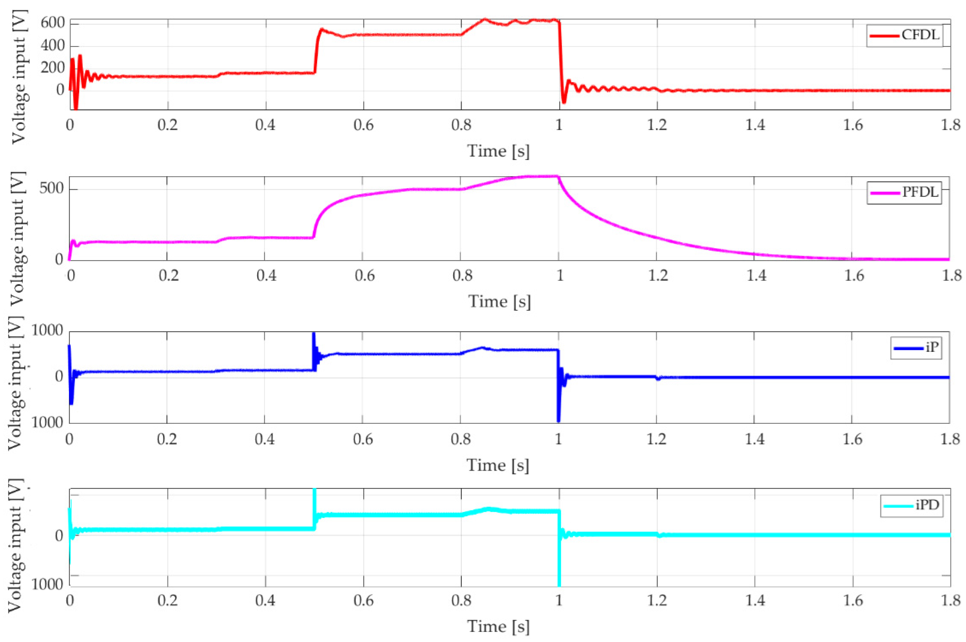
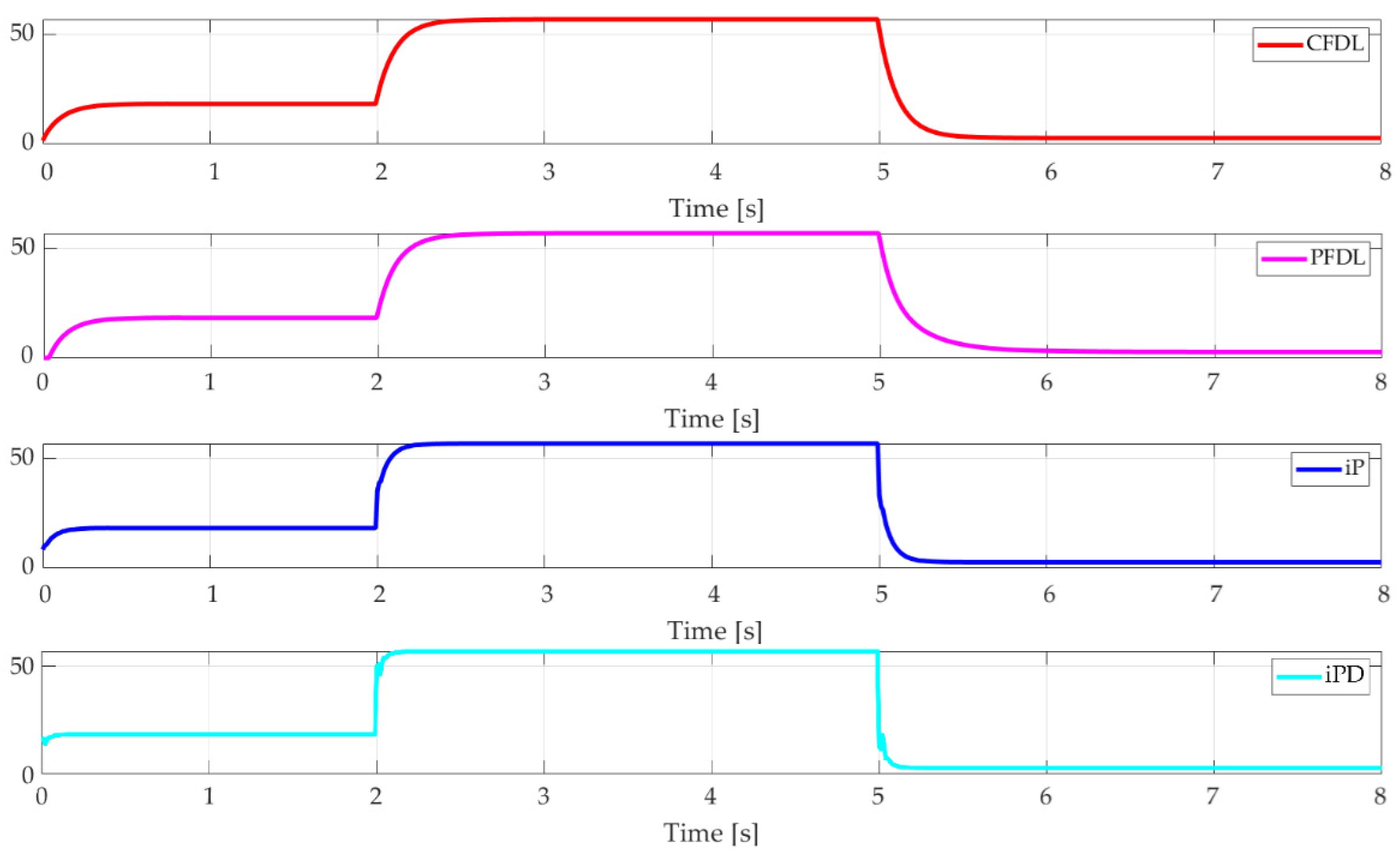
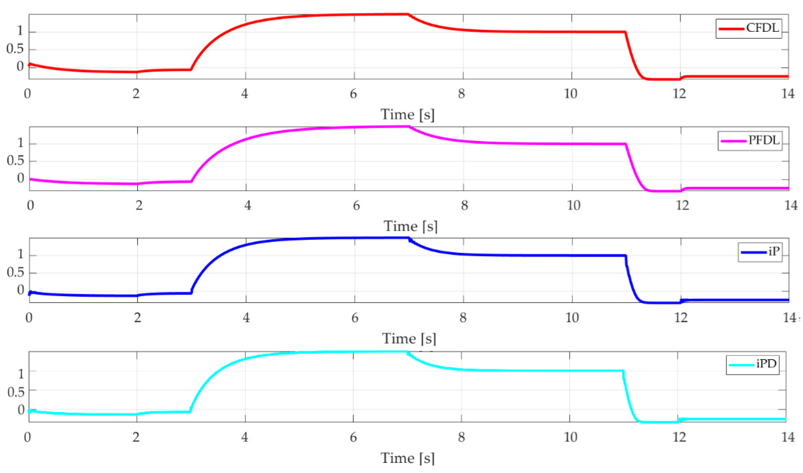
For the gradient-based approach, MFAC algorithms employing compact form dynamic linearization (CFDL) and partial form dynamic linearization (PFDL) were developed to optimize the initial values of time-varying parameters (PPD and PG), resulting in enhanced dynamic performance. On the other hand, the non-gradient-based MFC approach utilized intelligent proportional (iP) and intelligent proportional-derivative (iPD) controllers, which exhibit behavior analogous to classical PI and PID controllers. Both MFAC and MFC variants were tested and validated on nonlinear systems, enabling a direct performance comparison between the two methodologies.

Regarding the comparative analysis between MFAC and MFC, the results clearly indicate that MFC algorithms outperform their MFAC counterparts. While MFAC algorithms, both in CFDL and PFDL forms, exhibited slower responses and higher control errors, MFC algorithms demonstrated faster settling times, reduced overshoot, and lowered control errors, as evidenced by the discrete-time integral absolute error criterion. Both approaches successfully achieved steady-state error, rejected disturbances, and adapted to time-varying nonlinear systems. However, MFC algorithms consistently achieved control objectives more efficiently and with greater consistency in settling times. In contrast, MFAC algorithms, despite their adaptability, proved less efficient under significant reference value changes and introduced vulnerabilities in system perception due to dynamic linearization. The ultralocal model used in MFC, on the other hand, emerged as a more robust solution for online system estimation.

As a future research direction, the study proposes expanding the comparative analysis to include a wider range of systems with varied dynamics. Additionally, further validation of the proposed algorithms on a larger number of systems is recommended to solidify their applicability and effectiveness across diverse control scenarios.

References

1. Hou, Z.-S.; Wang, Z. From model-based control to data-driven control: Survey, classification and perspective. Inf. Sci. 2013, 235, 3–35. [Google Scholar] [CrossRef]
2. Tang, W.; Daoutidis, P. Data-Driven Control: Overview and Perspectives. In Proceedings of the 2022 American Control Conference (ACC), Atlanta, GA, USA, 8–10 June 2022; pp. 1048–1064. [Google Scholar]
3. Hjalmarsson, H.; Gevers, M.; Gunnarsson, S.; Lequin, O. Iterative feedback tuning: Theory and applications. IEEE Control Syst. Mag. 1998, 18, 26–41. [Google Scholar]
4. Huo, B.; Freeman, C.T.; Liu, Y. Model-free Gradient Iterative Learning Control for Non-linear Systems. IFAC-PapersOnLine 2019, 52, 304–309. [Google Scholar] [CrossRef]
5. Karimi, A.; van Heusden, K.; Bonvin, D. Non-iterative data-driven controller tuning using the correlation approach. In Proceedings of the 2007 European Control Conference (ECC), Kos, Greece, 2–5 July 2007; pp. 5189–5195. [Google Scholar]
6. Campi, M.C.; Lecchini, A.; Savaresi, S.M. Virtual reference feedback tuning: A direct method for the design of feedback controllers. Automatic 2002, 38, 1337–1346. [Google Scholar] [CrossRef]
7. Hou, Z.; Jin, S. Model Free Adaptive Control: Theory and Applications, 1st ed.; CRC Press: Boca Raton, FL, USA, 2016. [Google Scholar]
8. Fliess, M.; Join, C. Model free control. Int. J. Control 2013, 86, 2228–2252. [Google Scholar] [CrossRef]
9. Karimi, A.; Mišković, L.; Bonvin, D. Convergence Analysis of an Iterative Correlation-Based Controller Tuning Method. IFAC Proc. Vol. 2002, 35, 413–418. [Google Scholar] [CrossRef]
10. van Helvoort, J.; de Jager, B.; Steinbuch, M. Data-Driven Controller Unfalsification with Analytic Update Applied to a Motion System. IEEE Trans. Control Syst. Technol. 2008, 16, 1207–1217. [Google Scholar] [CrossRef]
11. Wang, Y.; Shen, C.; Huang, J.; Chen, H. Model-free adaptive control for unmanned surface vessels: A literature review. Syst. Sci. Control Eng. 2024, 12, 2316170. [Google Scholar] [CrossRef]
12. Dong, N.; Lv, W.; Zhu, S.; Gao, Z. Model-free adaptive nonlinear control of the absorption refrigeration system. Nonlinear Dyn. 2022, 107, 1623–1635. [Google Scholar] [CrossRef]
13. Heydari, M.; Darvishpoor, S.; Novinzadeh, A.B.; Roshanian, J. On the Performance of the Model-Free Adaptive Control For A Novel Moving-Mass Controlled Flying Robot. J. Intell. Robot. Syst. 2024, 110, 79. [Google Scholar] [CrossRef]
14. Zhao, L.; He, W.; Lv, F. Model-Free Adaptive Control for Parafoil Systems Based on the Iterative Feedback Tuning Method. IEEE Access 2021, 9, 35900–35914. [Google Scholar] [CrossRef]
15. Wu, L.; Li, Z.; Liu, S.; Li, Z.; Sun, D. A Novel Multi-Agent Model-Free Adaptive Control Algorithm for a Class of Multivehicle Systems with Constraints. Symmetry 2023, 15, 168. [Google Scholar] [CrossRef]
16. Yuan, D.; Wang, Y. Data Driven Model-Free Adaptive Control Method for Quadrotor Formation Trajectory Tracking Based on RISE and ISMC Algorithm. Sensors 2021, 21, 1289. [Google Scholar] [CrossRef] [PubMed]
17. Yang, Z.; Yu, X.; Jin, S.; Hou, Z. Model Free Adaptive Attitude Control of Launch Vehicle Using Iterative Feedback Tuning. In Proceedings of the 2019 IEEE 8th Data Driven Control and Learning Systems Conference (DDCLS), Dali, China, 24–27 May 2019; pp. 1196–1201. [Google Scholar]
18. Wang, D. A Novel Controller Dynamic Linearization-Based Model Free Adaptive Predictive Control for a Class of Discrete Nonlinear Systems. In Proceedings of the 2018 International Conference on Mechanical, Electronic, Control and Automation Engineering (MECAE 2018), Qingdao, China, 30–31 March 2018; pp. 413–421. [Google Scholar]
19. Corradini, M.L. A Robust Sliding-Mode Based Data-Driven Model-Free Adaptive Controller. IEEE Control Syst. Lett. 2022, 6, 421–427. [Google Scholar] [CrossRef]
20. Liu, W.; Ye, H.; Yang, X. Model-Free Adaptive Sliding Mode Control Method for Unmanned Surface Vehicle Course Control. J. Mar. Sci. Eng. 2023, 11, 1904. [Google Scholar] [CrossRef]
21. Madadi, E.; Söffker, D. Model-free control of unknown nonlinear systems using an iterative learning concept: Theoretical development and experimental validation. Nonlinear Dyn. 2018, 94, 1151–1163. [Google Scholar] [CrossRef]
22. Wang, J.; Wang, J.; Wang, X. Model Free Adaptive Sliding Mode Fault Tolerant Control for a 3-DOF Helicopter. In Proceedings of the 2022 IEEE International Conference on Unmanned Systems (ICUS), Guangzhou, China, 28–30 October 2022; pp. 1345–1349. [Google Scholar]
23. Roman, R.; Radac, M.; Precup, R.; Petriu, E.M. Data-driven Model-Free Adaptive Control Tuned by Virtual Reference Feedback Tuning. Acta Polytech. Hung. 2016, 13, 83–96. [Google Scholar]
24. Zhang, X.; Ma, H. Data-Driven Model-Free Adaptive Control Based on Error Minimized Regularized Online Sequential Extreme Learning Machine. Energies 2019, 12, 3241. [Google Scholar] [CrossRef]
25. Moreno-Gonzalez, M.; Artuñedo, A.; Join, C.; Fliess, M. Speed-Adaptive Model-Free Lateral Control for Automated Cars. IFAC-PapersOnLine 2022, 55, 84–89. [Google Scholar] [CrossRef]
26. Join, C.; Abouaïssa, H.; Fliess, M. Ramp Metering: Modeling, Simulations and Control Issues. Adv. Delays Dyn. 2022, 14, 227. [Google Scholar]
27. Lafont, F.; Balmat, J.-F.; Join, C.; Fliess, M. First steps toward a simple but efficient model-free control synthesis for variable-speed wind turbines. Int. J. Circuits Syst. Signal Process. 2020, 14, 1181–1191. [Google Scholar] [CrossRef]
28. Clouatre, M.; Thitsa, M.; Fliess, M.; Join, C. A robust but easily implementable remote control for quadrotors: Experimental acrobatic flight tests. In Proceedings of the 9th International Conference on Advanced Technologies (ICAT’20), Istanbul, Turkey, 10–12 August 2020. [Google Scholar]
29. Villagra, J.; Join, C.; Haber, R.; Fliess, M. Model-free control for machine tools. arXiv 2020, arXiv:2005.08546. [Google Scholar]
30. Michel, L. Model-free control of non-minimum phase systems and switched systems. arXiv 2011, arXiv:1106.1697. [Google Scholar]
31. Precup, R.-E.; Roman, R.-C.; Safaei, A. Data-Driven Model-Free Controllers, 1st ed.; CRC Press: Boca Raton, FL, USA, 2021. [Google Scholar]
32. Roman, R.-C.; Radac, M.-B.; Precup, R.-E.; Petriu, E.M. Virtual Reference Feedback Tuning of Model-Free Control Algorithms for Servo Systems. Machines 2017, 5, 25. [Google Scholar] [CrossRef]
33. Baciu, A.; Lazar, C. Iterative Feedback Tuning of Model-Free Intelligent PID Controllers. Actuators 2023, 12, 56. [Google Scholar] [CrossRef]
34. Li, W.; Yuan, H.; Li, S.; Zhu, J. A Revisit to Model-Free Control. IEEE Trans. Power Electron. 2022, 37, 14408–14421. [Google Scholar] [CrossRef]
35. Delaleau, E. A Proof of Stability of Model-Free Control. In Proceedings of the 2014 IEEE Conference on Norbert Wiener in the 21st Century (21CW), Boston, MA, USA, 24–26 June 2014. [Google Scholar]
36. Baciu, A.; Lazar, C. Parameters setting of a Data-Driven Model-Free Adaptive Controller for a coupled Two-Tank System. In Proceedings of the 2022 26th International Conference on System Theory, Control and Computing (ICSTCC), Sinaia, Romania, 19–21 October 2022; pp. 397–402. [Google Scholar]
37. Ren, C.; Zhang, J.; Hu, L.; Ma, S. Practical issues in data-driven model-free adaptive control for an omnidirectional mobile manipulator. ISA Trans. 2023, 142, 615–625. [Google Scholar] [CrossRef]
38. Lewis, F.L. Applied Optimal Control and Estimation: Digital Design and Implementation; Pretince-Hall: Hoboken, NJ, USA, 1992. [Google Scholar]
39. Benidir, M. On the root distribution of general polynomials with respect to the unit circle. Signal Process. 1996, 53, 75–82. [Google Scholar] [CrossRef]
40. Jeon, Y.S.; Mok, H.S.; Choe, G.H.; Kim, D.K.; Ryu, J.S. A new simulation model of BLDC motor with real back EMF waveform. In Proceedings of the COMPEL 2000 7th Workshop on Computers in Power Electronics, Blacksburg, VA, USA, 16–18 July 2000; pp. 217–220. [Google Scholar]
41. Narendra, K.S.; Parthasarathy, K. Identification and control of dynamical systems using neural networks. IEEE Trans. Neural Netw. 1990, 1, 4–27. [Google Scholar] [CrossRef]
42. Jin, L.; Nikiforuk, P.N.; Gupta, M.M. Adaptive control of discrete-time nonlinear systems using recurrent neural networks. IEE Proc.-Control Theory Appl. 1994, 141, 169–176. [Google Scholar] [CrossRef]
43. Baciu, A.; Lazar, C. Experimental Comparison of Two Data-Driven Algorithms for Pitch Control of an Aerospace System. In Proceedings of the 2023 31st Mediterranean Conference on Control and Automation (MED), Limassol, Cyprus, 26–29 June 2023; pp. 329–334. [Google Scholar]
Figure 1. Average absolute error for steps variation during Algorithm 1 for BLDC motor.
Applsci 15 02766 g001
Figure 2. BLDC motor speed for CFDL optimization algorithm.
Applsci 15 02766 g002
Figure 3. Average absolute error for steps variation during Algorithm 1 for non-minimum phase nonlinear system.
Applsci 15 02766 g003
Figure 4. Output signals for CFDL optimization algorithm applied for non-minimum phase nonlinear system.
Applsci 15 02766 g004
Figure 5. Average absolute error steps variation during Algorithm 1 for nonlinear system with time-varying parameter.
Applsci 15 02766 g005
Figure 6. Output signals for CFDL optimization algorithm applied for nonlinear system with time-varying parameter.
Applsci 15 02766 g006
Figure 7. Average absolute error steps variation during Algorithm 2 for BLDC motor.
Applsci 15 02766 g007
Figure 8. BLDC motor speed for PFDL optimization algorithm.
Applsci 15 02766 g008
Figure 9. Average absolute error steps variation during Algorithm 2 for nonminimum phase nonlinear system.
Applsci 15 02766 g009
Figure 10. Output signals for PFDL optimization algorithm applied for nonminimum phase nonlinear system.
Applsci 15 02766 g010
Figure 11. Average absolute error steps variation during Algorithm 2 for nonlinear system with time-varying parameter.
Applsci 15 02766 g011
Figure 12. Output signals for PFDL optimization algorithm applied for nonlinear system with time-varying parameter.
Applsci 15 02766 g012
Figure 13. Load torque applied to BLDC motor.
Applsci 15 02766 g013
Figure 14. Speed of BLDC motor for CFDL, PFDL, iP, iPD comparison.
Applsci 15 02766 g014
Figure 15. Speed of BLDC motor for CFDL, PFDL, iP, iPD comparison—detailed view.
Applsci 15 02766 g015
Figure 16. Voltage input signal of BLDC motor for CFDL, PFDL, iP, iPD comparison.
Applsci 15 02766 g016
Figure 17. Output signals of nonminimum phase nonlinear system.
Applsci 15 02766 g017
Figure 18. Output signals of nonminimum phase nonlinear system—detailed view.
Applsci 15 02766 g018
Figure 19. Control signals of nonminimum phase nonlinear system.
Applsci 15 02766 g019
Figure 20. Output signals for nonlinear system with time-varying parameter.
Applsci 15 02766 g020
Figure 21. Output signals for nonlinear system with time-varying parameter—detailed view.
Applsci 15 02766 g021
Figure 22. Control signals for nonlinear system with time-varying parameter.
Applsci 15 02766 g022