Parameter Sensitivity Analysis of Generators and Grid-Connected Constraints in Hybrid Microgrids Using Deep Reinforcement Learning

Abstract

Hybrid renewable energy systems, which combine photovoltaic panels, wind turbines, batteries, generators, and grid connections, require careful sizing to balance economic performance, renewable integration, and supply reliability. In this context, this study proposes a deep reinforcement learning (DRL)-based sensitivity analysis framework in which the admissible energy contributions from the diesel generator and the grid are treated as explicit design-control parameters. The objective is to simultaneously minimize the levelized cost of energy, minimize the loss of power supply probability, and maximize the renewable energy fraction. A sensitivity analysis was conducted across different HRES configurations, load profiles, and tau/gamma values. The performance of the DRL approach was compared with that of multi-objective particle swarm optimization and the non-dominated sorting genetic algorithm II under the same study setting. The results indicate that DRL can identify competitive trade-offs, especially under standard load conditions, while also providing insight into how admissible backup-energy constraints reshape techno-economic and reliability compromises. The best trade-offs were observed around intermediate tau and gamma values, suggesting that moderate backup-energy margins are more favorable than extreme values. These findings should be interpreted within the scope of a simulation-based study and provide comparative design-oriented evidence rather than universally transferable design rules.

1. Introduction

The decarbonization of power systems often necessitates the deployment of hybrid energy microgrids to mitigate the dependence on fossil fuels. These microgrids integrate renewable and conventional energy resources with energy storage capabilities, connecting directly to consumers and regulated by hybrid renewable energy systems (HRESs) to ensure efficient energy utilization and storage.

A parameter sensitivity analysis serves as a critical methodology for the design, optimization, and comprehensive assessment of HRES viability. This analytical approach facilitates the identification of parameters that exert significant influence on the technical, economic, and environmental performance of these systems. Recent scholarly investigations have focused on the impact of various hybrid configurations on the technical and financial viability of HRESs, frequently employing simulation models to address inherent uncertainties [1,2,3,4,5]. The primary sources of uncertainty within HRESs include the following:

• The intrinsic variability in renewable resources, such as the solar irradiance and wind speed [1,2].
• Fluctuations in the load demand [3,6].
• Financial variables, including the cost of capital and the energy discount rate [2,3,4,7].
• The operational lifespan of system equipment [2,3,4].
• Variations in energy pricing [8,9].
• Equipment failure rates [1,2,8,9].

Analyses of renewable resources indicate that variations in solar insolation and wind velocity significantly impact the system configuration and, consequently, the levelized cost of energy (LCOE) [1,2,9]. Furthermore, research has consistently demonstrated that the lifespan of system components, the annual average wind speed, and the average annual solar irradiance have a significant impact on the energy costs and system reliability. There are also reports highlighting that the integration of diverse renewable sources increases the share of renewable energy and reduces the reliance on diesel generators, thereby contributing to an enhanced HRES reliability [4,7,8,9].

Regarding the economic aspects and profitability of HRESs, it has been established that a reduction in the proportion of renewable resources can decrease the LCOE [3,6,8]. Conversely, an increase in the load demand or ambient temperatures tends to escalate the LCOE [6]. These studies collectively suggest that discount rates and investment costs exert a substantial influence on the profitability and sizing of HRESs. Notably, 100% renewable systems have demonstrated the potential for cost reductions exceeding 30% when compared to traditional power system configurations [5,7,9].

Table 1. Summary of work on sensitivity analysis.

Study Endpoint	Impact Observed	References
Solar irradiance/wind speed resources	Energy cost, system size	[1,3,5,8,9]
Discount rate	Cost-effectiveness, optimal configuration	[1,3,8,9,10]
Component life	Total cost, replacement frequency	[1,2,8,9]
Energy prices (grid-connected)	Economic viability	[2,3,6,8,9]
Request for a charge	Sizing, operating cost	[2,5,6,7,10]
Environmental policies	Total cost, choice of technologies/resources	[8]

summarizes the sensitive parameters commonly analyzed in the numerous studies presented in the literature.

A parameter sensitivity analysis is essential for ensuring the viability of HRESs. It accounts for uncertainties such as resource variability and fluctuating load demands while also considering specific requirements, including critical load priorities and desired energy autonomy levels [5,7,8]. This analysis can also facilitate the sale of surplus energy to the grid, helping to maximize the renewable penetration and profitability [3,6]. However, the current approaches often overlook two key aspects:

• The HRES sensitivity to emergency energy constraints: To minimize the carbon footprint, it is crucial to limit reliance on generators or the main grid. In many deep reinforcement learning (DRL) applications, this limit is often implicitly below 5% or entirely absent [11]. A thorough exploration is needed to understand how system policies adapt when this hyperparameter is relaxed during scaling.
• Dynamic economic sizing and associated risks: The real-time spot price signals and the inherent volatility of renewable resources demand risk-aware planning. While recent research has proposed risk-sensitive deep reinforcement learning using the conditional value at risk (CVaR) [12], its applications within HRES contexts remain limited.

Traditionally, HRES sizing relied on meta-heuristics such as multi-objective particle swarm optimization (MOPSO) and the non-dominated sorting genetic algorithm II (NSGA-II). However, recent advancements in DRL are revolutionizing this field. DRL enables real-time policy learning that inherently accounts for system dynamics, shifting control from rigid rule-based or forecast-driven approaches to autonomous, adaptive decision-making, even in complex and uncertain environments.

Several DRL algorithms have become prominent in this domain. The twin delayed deep deterministic policy gradient (TD3) aims to prevent the overestimation of action values through twin Q-networks and delayed policy updates [13]. Soft actor–critic (SAC), on the other hand, prioritizes maximizing the policy entropy to encourage the exploration of diverse control strategies [14]. A hierarchical deep Q-network (HDQN) stands out with its hierarchical policy structure, making it particularly well-suited for learning across different decision levels, such as distinguishing between operational control and strategic system sizing [15].

Despite these advancements, a critical gap remains in the research: the sensitivity of HRESs to emergency energy constraints. While DRL applications for HRESs have largely focused on cost reduction and renewable energy integration, the impact of a permissible load demand from generators and the main grid on system design is often overlooked. It is crucial to understand how varying levels of contribution from diesel generators (DG) and the electrical power grid (GRID) affect the reliability and cost of HRESs, especially for designing resilient systems. Unfortunately, this vital constraint is frequently neglected, particularly in models that lack dynamic penalties for insufficient backup power. Furthermore, while classical sensitivity methods are commonly applied in power grids, their use in hybrid systems remains limited [16,17]. This study aimed to address this critical gap by comprehensively analyzing the sensitivity of HRESs to backup-energy constraints. Our goal was to identify crucial trade-offs and anticipate the risks associated with resource variability and operational constraints.

This manuscript is related to our earlier paper [18], but its objective is different and more specific. The previous study primarily established the feasibility of using a DRL-based framework for hybrid renewable energy system sizing under a general multi-criteria setting. In that earlier work, backup sources such as the diesel generator and the utility grid were part of the overall sizing environment, but they were not the central analytical axis of the study.

In contrast, the present manuscript focuses specifically on the sensitivity of HRES design to admissible backup-energy contributions. More precisely, the main originality of this paper lies in treating the generator and grid contribution ratios, denoted by $\tau$ and $\gamma$, as explicit design-control parameters and in analyzing how these parameters reshape the trade-offs among LCOE, LPSP, and REF. Accordingly, the contribution here is not simply an additional application of DRL, but a constraint-aware sensitivity analysis framework, complemented by a structured benchmark against MOPSO and NSGA-II, with the aim of extracting design-oriented insights on the role of backup-energy flexibility in HRES planning.

Our key contributions are as follows:

• A sensitivity analysis framework in which tau and gamma are modeled as explicit admissible contribution ratios for the generator and the grid, allowing for backup-energy dependence to be studied as a design variable.
• A DRL-based constrained optimization approach with a cumulative reward that jointly accounts for LCOE minimization, LPSP minimization, REF maximization, and penalties associated with excessive reliance on backup sources.
• A structured multi-objective benchmark against MOPSO and NSGA-II, enabling a comparative discussion of where DRL is advantageous, where evolutionary baselines remain more conservative, and how admissible backup constraints reshape the compromise between the cost, reliability, and renewable integration.

A parameter sensitivity analysis of DG/GRID contributions is crucial for optimizing the sizing of HRESs. It allows us to test the robustness of a given configuration under real-world uncertainties. This analysis helps identify key parameters, such as the allowable percentage of energy input from the generator and the main grid, which significantly influence the values of the LCOE, LPSP, and REF, especially under various constraints. Ultimately, it highlights how resource variability and economic factors shape the design choices for a truly sustainable energy transition.

This article is structured as follows: Section 2 details the study’s methodology, including a comprehensive presentation of the proposed DRL approach, comparative methods, and experimental design. Section 3 presents the study’s results and compares the different methodologies. The article concludes with a summary and outlines future research directions.

2. System Modeling

This research includes a sensitivity analysis of HRESs. This section establishes the conceptual and experimental framework for the analysis of diesel generator and grid configurations in hybrid microgrids. We structured it into three subsections: the formulation of the optimization problem, modeling using DRL, and the design of the numerical experiment. The core objective of this study was to leverage an intelligent agent to discover beneficial energy distribution strategies. These strategies were designed to satisfy critical reliability constraints, such as limiting the emergency energy supply from the generator and the main grid. Simultaneously, the goal was to maximize renewable energy penetration and minimize the operating costs. A key part of this study also involved examining how different allowable limits for these emergency sources impact the system’s overall performance.

2.1. HRES Configurations

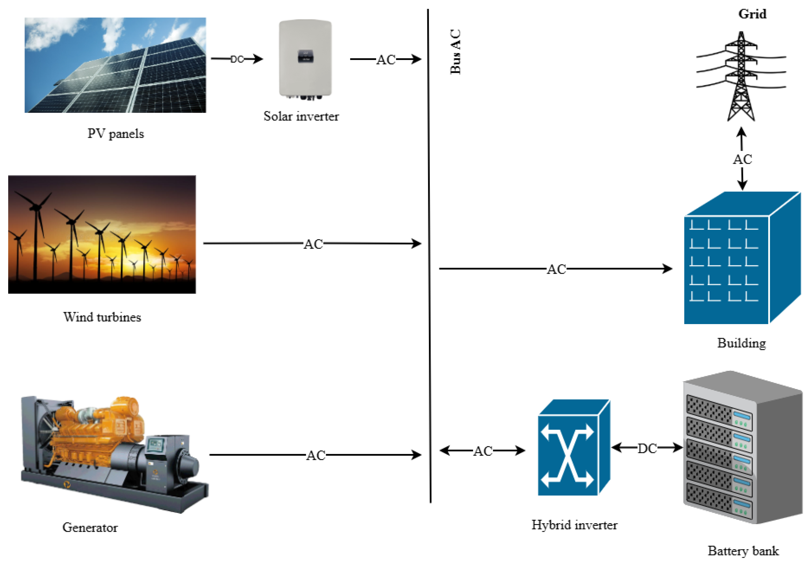
For clarity, Figure 1 was created for this manuscript to reflect the updated simulated system design; the earlier configuration is described in [18].

In the context of this sensitivity analysis, the study supports the following hypothesis: the constituents of the system that meet one need differ from those that meet another. These systems consist of photovoltaic (PV) panels, wind turbines (WTs), a battery energy storage system (BESS), and possibly a diesel generator (DG).

Indeed, Kushwaha and Bhattacharjee [19] highlighted the importance of choosing the right HRES components. The results of their study on the comparison of different types of systems that include PV panels, WTs, a BESS, a DG, and/or a biogas generator (BG) revealed the PV + WT + BESS + BG + DG system to be best suited in their context. Similarly, the study by Mokhtara, Negrou et al. [20] showed that the most suitable system for electrifying a residential building in a rural environment is PV + WT + BESS + DG.

Therefore, to ensure an exhaustive analysis, this study considered four (4) types of hybrid renewable energy systems:

• PV panels coupled with a BESS: PV + BESS.
• PV panels coupled with a BESS and a DG: PV + BESS + DG.
• PV panels coupled with WTs and a BESS: PV + WT + BESS.
• PV panels coupled with WTs, a BESS, and a DG: PV + WT + BESS + DG.

Table 2. Technical parameters used for the main HRES components.

Component	Parameter	Value	Unit
PV	Rated output power	200	W
PV	Cell efficiency	22.90	%
PV	NOCT	45	°C
PV	Lifetime	25	years
WT	Rated power	1	kW
WT	Cut-in/cut-out speed	2.5/20	m/s
WT	Rated speed	11	m/s
WT	Lifetime	30	years
BESS	$SO{C}_{min}$/$SO{C}_{max}$	10/100	%
BESS	Charge/discharge efficiency	92	%
BESS	Self-discharge rate	0.01	%
BESS	Lifetime	15	years
DG	Candidate capacities	7.5–24	kW
DG	Fuel cost	1.2	$/L
DG	Lifetime	25	years

summarizes the technical and techno-economic parameters used for the main HRES components. These values follow the component assumptions adopted in the present study and are consistent with the system modeling framework reported in our earlier DRL work [18].

Figure 1 illustrates an HRES that integrates photovoltaic panels, wind turbines, battery energy storage systems, and a generator. A bidirectional inverter facilitates the conversion of battery energy to loads and the storage of surplus energy, serving a dual purpose. A hybrid inverter converts DC energy from the PV panels into usable AC power for the loads. The system also connects to a generator, providing power during periods of the underproduction of renewable energy.

The power grid maintains a bidirectional connection to the loads, enabling two functions: supplying energy when the demand exceeds the renewable production and exporting surplus energy to the grid when storage is not feasible.

At each hourly time step, the energy balance is enforced by prioritizing renewable generation and then activating storage and backup sources when needed. When the renewable production exceeds the load demand, the surplus is first directed to battery charging subject to the converter efficiency and storage limits; if the battery is already full, the remaining surplus may be exported to the grid when grid export is allowed. Conversely, when the renewable production is lower than the demand, the deficit is covered sequentially by the battery and then by the diesel generator and/or the grid within the admissible limits defined by tau and gamma. Conversion losses are accounted for through the inverter and storage efficiencies, while any remaining unmet demand contributes directly to the LPSP metric.

The core challenge of this study lies in balancing two conflicting objectives: minimizing the reliance on external sources for decarbonization while maintaining an acceptable level of supply security, especially during renewable energy deficits. Backup energy bridges the gap between the demand and the available renewable sources (PV + WT + BESS). However, this backup must remain below a critical threshold to prevent excessive fossil fuel use and foster resilient, autonomous systems.

Therefore, this study addressed a dynamic optimization problem of energy dispatch between various sources. The primary goal was to minimize the LCOE while adhering to strict constraints on the DG and GRID contributions and ensuring system robustness. This optimization is complex due to the inherent uncertainty of renewable generation (PV + WT), a fluctuating demand, and nonlinear interactions between microgrid components.

2.2. System Performance Metrics

The levelized cost of energy (LCOE), renewable energy fraction (REF), and loss of power supply probability (LPSP) are often used as HRES performance metrics. Their role is as follows:

• The LCOE measures the economic performance of an HRES [21,22];
• The REF quantifies the level of renewable integration within the microgrid [23];
• The LPSP indicates the reliability of an HRES [23,24].

This study considered these three performance indicators for their ability to offer a balanced approach to HRES evaluation. More specifically, the LCOE provides a summary of all the investment, operating, and maintenance costs over the system’s lifetime. The LPSP provides a quantitative measure of the probability of energy failure. This measure ensures that the critical needs remain covered, even in the event of fluctuating resources. Finally, the REF serves as an indicator of the proportion of energy from renewable sources. The REF thus provides a measure of a system’s effectiveness in minimizing the dependence on fossil fuels and reducing its carbon footprint.

2.2.1. Levelized Cost of Energy

The levelized cost of energy is a tool used as an indicator for comparing the lifetime costs of the electricity production of different energy technologies $\left(m_j\right)$. This measure is widely used in the literature to assess the economic competitiveness of renewable and conventional energy [21,22,25,26].

The LCOE is highly dependent on the discount rate, initial capital costs, operating costs, effective lifetime of the installation $\left(m_s\right)$, and energy efficiency [21,25]. The LCOE, expressed in $/kWh, is represented by Equation (1) [21]:

$$\mathrm{LCOE}={\displaystyle \frac{{\mathbb{C}}_{\mathrm{Total}}}{{\sum }_{t=1}^{8760}{P}_L\left(t\right)}}$$

(1)

with

$${\mathbb{C}}_{\mathrm{Total}}={\mathbb{C}}_{\mathrm{Capital}}+{\mathbb{C}}_{\mathrm{Remp}}+{\mathbb{C}}_{\mathrm{Op}\&\mathrm{Maint}}+E_a\times \vartheta -E_v\times \min (\vartheta ,\mu )$$

(2)

where ${\mathbb{C}}_{\mathrm{Total}}$ represents the total investment cost over the entire project life. This cost includes the initial investment cost $\left({\mathbb{C}}_{\mathrm{Capital}}\right)$, replacement costs $\left({\mathbb{C}}_{\mathrm{Remp}}\right)$, maintenance and operation costs $\left({\mathbb{C}}_{\mathrm{Op}\&\mathrm{Maint}}\right)$, and the costs of purchasing energy from the grid $(E_a\times \vartheta )$ subtracted from the costs of selling energy on the grid $(E_v\times \min (\vartheta ,\mu ))$. $E_a$ and $E_v$ are, respectively, the total quantities of energy purchased and sold on the electricity grid. $\vartheta$ represents the rate of purchase of energy, and $\mu$ is the rate of energy sales.

Table 3. Cost evaluation parameters.

Parameters	$\mathit{\vartheta }$ ($/kWh)	$\mathit{\mu }$ ($/kWh)	${\mathit{m}}_{\mathit{s}}$ (Years)
Value	0.14	0.05	25

presents the values of the parameters used in this study.

2.2.2. Renewable Energy Fraction

The REF, usually expressed as a percentage (%), is an indicator that measures the share of energy produced from renewable sources in each energy system. For this study, the REF focuses on the amount of energy produced by the PV source in PV + BESS and PV + BESS + DG systems, as well as by the PV and WT sources for PV + WT + BESS and PV + WT + BESS + DG systems. The REF enables the quantification of progress toward more sustainable energy goals [23].

Considering a PV + WT + BESS + DG system attached to the grid, the REF is expressed by Equation (3). Combining the REF with the total system efficiency helps assess how an added renewable capacity reduces fossil fuel use [23]. This study specifically reflects the reduction in diesel generator energy input.

$$\begin{array}{c}\mathrm{REF}={\displaystyle \frac{{\sum }_{t=1}^{8760}{P}_{\mathrm{renewable}}\left(t\right)}{{\sum }_{t=1}^{8760}{P}_{\mathrm{Total}}\left(t\right)}}={\displaystyle \frac{{\sum }_{t=1}^{8760}\left(P_{\mathrm{WT}}\left(t\right)+{\eta }_{\mathrm{PV}}\times P_{\mathrm{PV}}\left(t\right)\right)}{{\sum }_{t=1}^{8760}\left(P_{\mathrm{WT}}\left(t\right)+{\eta }_{\mathrm{PV}}\times P_{\mathrm{PV}}\left(t\right)+P_{\mathrm{GRID}}\left(t\right)+P_{\mathrm{DG}}\left(t\right)\right)}}\\ \mathrm{REF}(\%)=\mathrm{REF}\times 100\end{array}$$

(3)

$P_{\mathrm{WT}}\left(t\right)$ and $P_{\mathrm{PV}}\left(t\right)$ represent the production from wind turbines and the production from PV panels, respectively, at time t. ${\eta }_{\mathrm{PV}}$ is the efficiency of the PV panels. This is a value provided by the manufacturer. $P_{\mathrm{GRID}}\left(t\right)$ and $P_{\mathrm{DG}}\left(t\right)$ represent the amount of power generated by the grid and the diesel generator at the same time t.

2.2.3. Loss of Power Supply Probability

The loss of power supply probability is a crucial indicator in electricity distribution and transmission systems, especially for integrating renewable energy and variable loads. The optimization of the LPSP enables the optimization of HRES management. It also improves the reliability of the system by incorporating the uncertainty related to the variability in loads and energy sources [24,27,28]. The LPSP is expressed in Equation (4) below [29]:

$$\begin{array}{c}\mathrm{LPSP}={\displaystyle \frac{{\sum }_{t=1}^{8760}\mathrm{LPS}\left(t\right)}{{\sum }_{t=1}^{8760}{P}_L\left(t\right)}}={\displaystyle \frac{{\sum }_{t=1}^{8760}\left(P_L\left(t\right)-P_{\mathrm{Total}}\left(t\right)\right)}{{\sum }_{t=1}^{8760}{P}_L\left(t\right)}}\\ \mathrm{LPSP}(\%)=\mathrm{LPSP}\times 100\end{array}$$

(4)

with $P_{\mathrm{Total}}\left(t\right)$ representing the total amount of energy supplied by the sources at time t. Thus, $\mathrm{LPS}\left(t\right)$ represents the energy loss recorded in time t.

2.3. Optimization Model

The optimization of the HRES in the context of this sensitivity analysis study is a multi-criteria optimization problem under uncertainties and constraints. The objectives of the optimization problem are the LCOE, the REF, and the LPSP, as described in the previous sections. Equation (5) presents the optimization problem to be solved under the constraints in Equation (6) [30]:

$$\begin{array}{c}\left\{\begin{array}{c}\min f_1=\min \mathrm{LCOE}\hfill \\ \min f_2=\min \mathrm{LPSP}\hfill \\ \max f_3=\max \mathrm{REF}\hfill \end{array}\right.\end{array}$$

(5)

$$\begin{array}{c}{P}_{\mathrm{GRID}}\le P_{\mathrm{GRID}}^{\max }=\gamma \times P_L\\ P_{\mathrm{DG}}\le P_{\mathrm{DG}}^{\max }=\tau \times P_L\\ \mathrm{LPSP}\le \epsilon =0.05\end{array}$$

(6)

with $\gamma ,\tau \in [0.1,0.2,0.3,0.4,0.5]$ (

Table 4. Decision variables and admissible control ranges considered in the sensitivity analysis.

Decision Variable	Symbol	Admissible Range/Description
Generator’s admissible contribution ratio	$\tau$	$\{0.1,0.2,0.3,0.4,0.5\}$
Grid’s admissible contribution ratio	$\gamma$	$\{0.1,0.2,0.3,0.4,0.5\}$
Number of PV panels	$N_{PV}$	0–50
Number of wind turbines	$N_{WT}$	0–50
Battery capacity	$Ca{p}_{BESS}$	$[0,100]\mathrm{kWh}$
Diesel generator capacity	$Ca{p}_{DG}$	Selected from the feasible configuration set generated from the candidate DG capacities listed in Table 2

) representing the percentages of allowable energy input via the grid and the diesel generator, respectively. $\epsilon$ represents the maximum acceptable value for the HRES reliability criterion.

The selected tau and gamma ranges were chosen to cover five interpretable operating regimes, from restrictive backup usage (0.1) to relatively permissive backup usage (0.5), while preserving a manageable sensitivity grid for comparative analysis. Values below 0.1 were considered overly restrictive for the selected study setting because they would sharply limit the corrective role of the backup sources, whereas values above 0.5 would reduce the practical meaning of the low-carbon design objective by allowing excessive dependence on external support. The adopted range therefore provides a balanced compromise between interpretability, feasibility, and computational tractability.

To analyze the sensitivity of HRESs to external power inputs, this study presents an enhanced experimental design. We examined the impact of contributions from diesel generators and the main grid on key metrics, including the LCOE, REF, and LPSP. This section begins by detailing the specific parameters under investigation and their varied ranges, as summarized in Table 4. Following this, we introduced the three primary evaluation methodologies utilized: DRL, MOPSO, and the NSGA-II.

2.4. Load Profiles

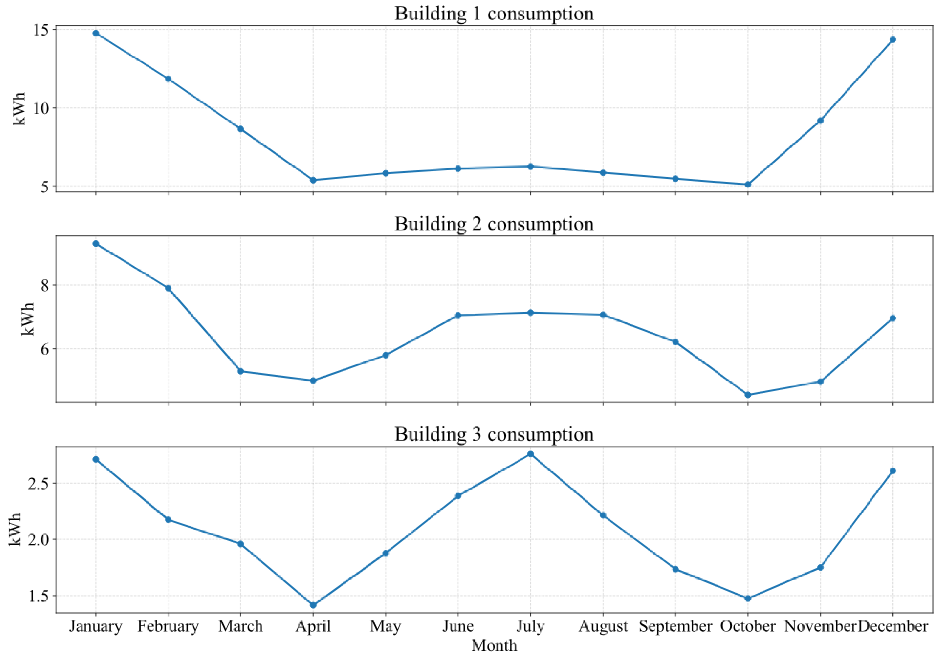
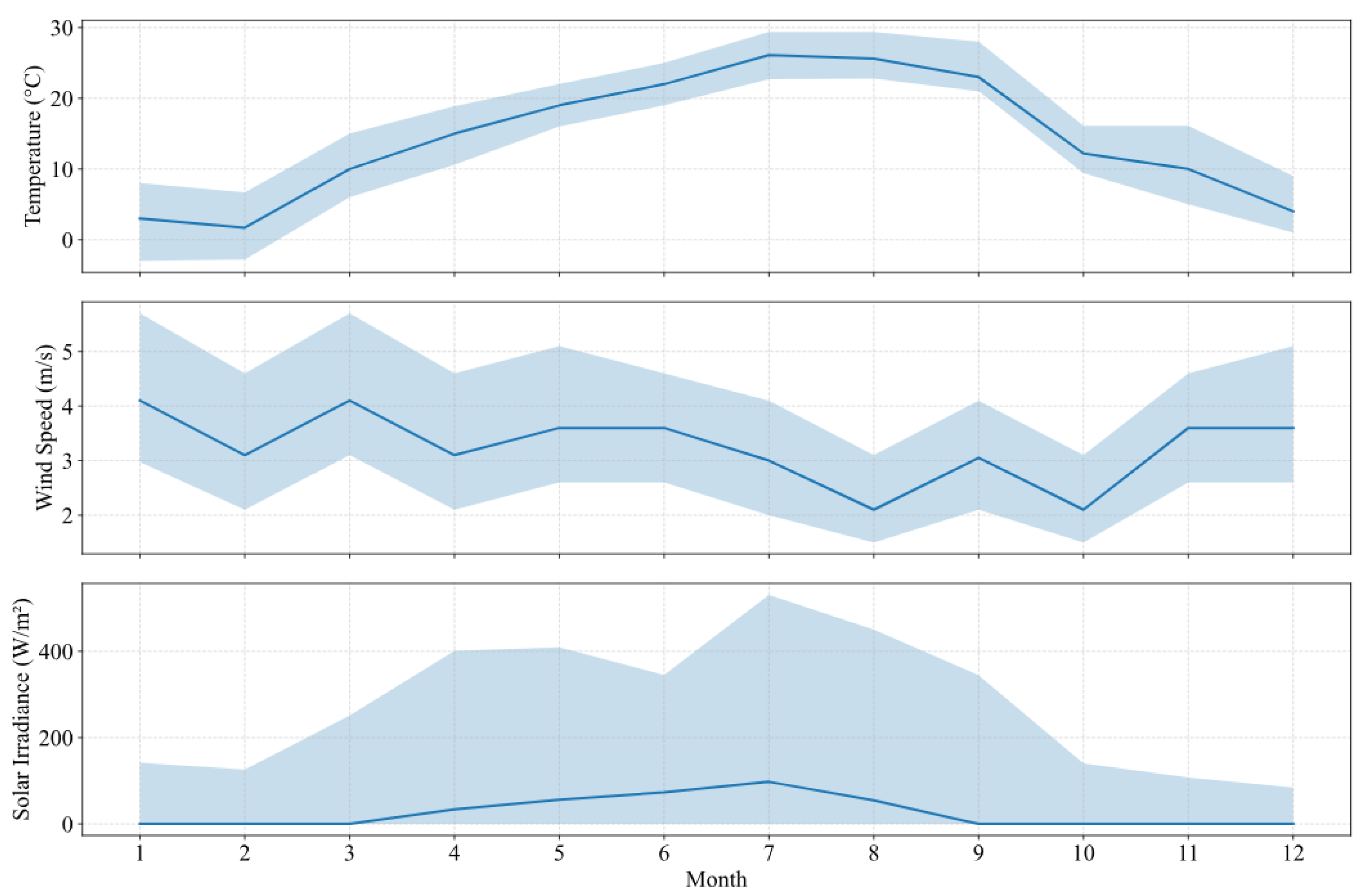
This study considered three load demand profiles (P1, P2, and P3) with significant variations ranging from 21.9% to 74.6% (Figure 2). These profiles, which exhibit high variation, represent the demands of three different types of buildings from the National Renewable Energy Laboratory (NREL) database. The aim of selecting these three buildings with contrasting profiles was to provide a rigorous analysis of the influence of load variability on the technical and economic performance of the HRES. This approach also ensures the optimal representativeness of real operating scenarios. However, in the context of this study, the same locality was considered. Thus, the climate data were the typical meteorological year (TMY) data of the said locality. The wind speed, solar irradiance, and temperature of this locality are shown in Figure 3. This figure illustrates the significant seasonal variability in wind and solar resources and temperatures throughout the year. This analysis of the source variability makes it possible to accurately assess the climatic impact on the HRES performance and reliability.

To improve clarity on the input data pipeline, all load and climatic series were organized on an hourly basis over one representative year (8760 time steps). The preprocessing stage consisted of aligning the NREL demand profiles and the TMY climatic variables on the same temporal grid, checking the unit consistency, and directly using the resulting hourly profiles as inputs to the HRES evaluation model. No ad hoc artificial measurements were introduced; instead, the reported results are simulation-derived values obtained from the adopted physical and techno-economic modeling framework.

In addition, this study evaluated four (4) types of HRESs: PV + BESS, PV + WT + BESS, PV + BESS + DG, and PV + WT + BESS + DG. The systems were evaluated for each type of profile to analyze the impact of each system type on the profiles and the associated analysis factors.

Table 5. Total demand per profile.

Profile	P1	P2	P3
Total demand (kWh)	72,157.99	56,341.69	18,317.89

shows the total demand for each profile.

For clarity, Figure 2 and Figure 3 were generated specifically for this manuscript from the study datasets and simulation setup (Section 2.5); earlier work [18] is cited for additional methodological details.

2.5. Solution Approach

This section outlines the methodologies employed to determine the best HRES configurations based on the LCOE, REF, and LPSP performance criteria.

The following subsections present the optimization and evaluation procedures adopted in the present study; additional methodological details are available in [18].

The manuscript emphasizes that the objective here is a sensitivity analysis rather than exhaustive algorithmic retuning. For this reason, the DRL training setting was kept unchanged across the tested scenarios so that the reported differences can be attributed to the load profiles, HRES configurations, and admissible backup-energy constraints rather than to changing the learning settings. Replay memory and a target network were used throughout the optimization to reduce the instability caused by sequentially correlated updates.

2.5.1. Deep Reinforcement Learning

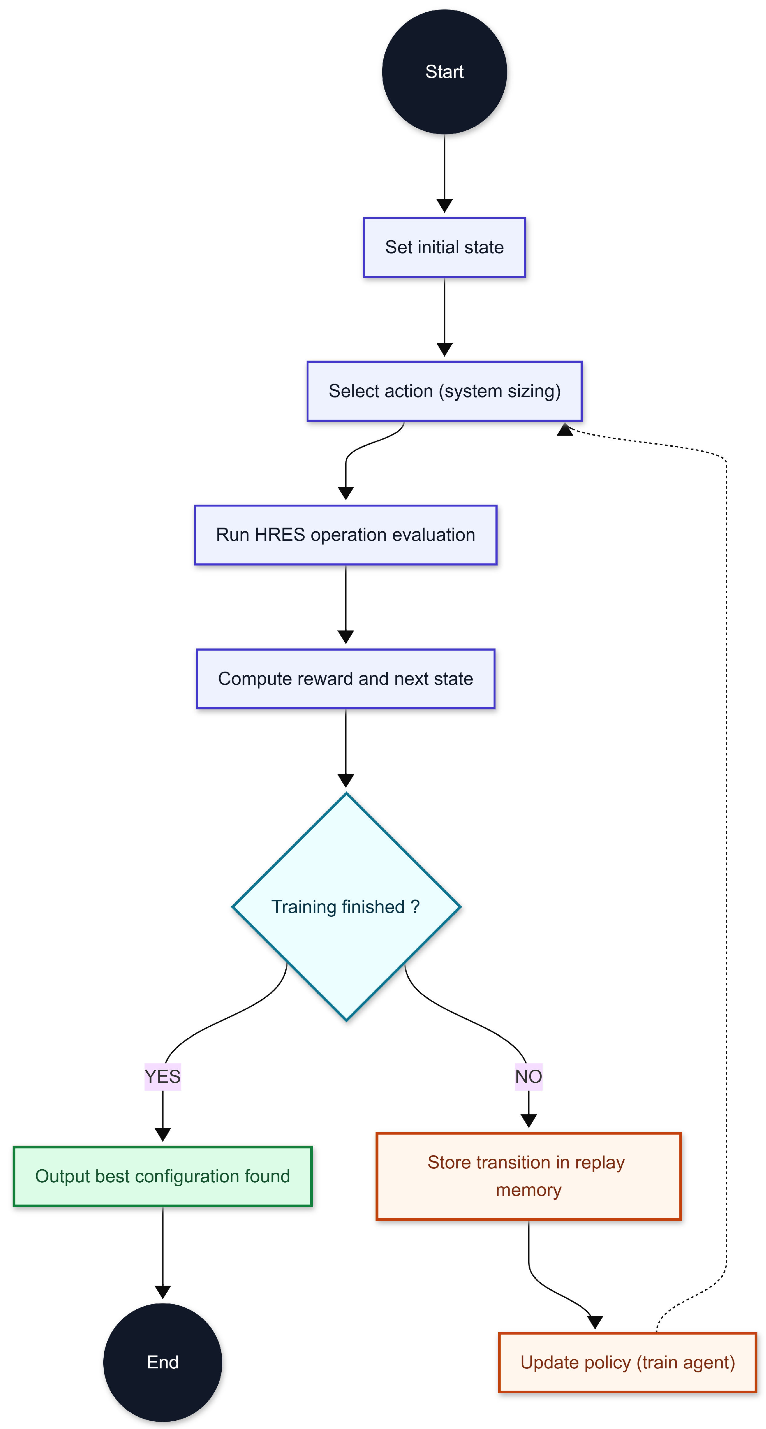
This study presents a multi-step DRL technique (Figure 4). This technique relies on a replay-memory and target-network training procedure designed to improve learning stability during sequential HRES evaluations. It begins with an initialization phase, where key system parameters are configured to establish the initial state vector at time step zero. As the process progresses, these parameter values are updated to determine the new state. The HRES state, denoted as S, is defined in Equation (7):

$$\mathrm{S}=\left\{N_{\mathrm{PV}},N_{\mathrm{WT}},{\mathrm{Cap}}_{\mathrm{BESS}},{\mathrm{Cap}}_{\mathrm{DG}},E_{\mathrm{np}},E_l,\mathrm{LCOE},\mathrm{LPSP},\mathrm{REF}\right\}$$

(7)

where $N_{\mathrm{PV}}$ and $N_{\mathrm{WT}}$ are the number of PV panels and wind turbines to be considered in each agent’s decision. ${\mathrm{Cap}}_{\mathrm{BESS}}$ and ${\mathrm{Cap}}_{\mathrm{DG}}$ represent the storage system’s capacity and the diesel generator’s capacity to be considered, respectively. $E_{\mathrm{np}}$ and $E_l$ are the amount of energy not supplied and the amount of energy lost over the entire evaluation period, i.e., over the lifetime of the HRES. Finally, LCOE, LPSP, and REF are the values of the factors measuring the quality of the DRL agent’s decision.

Following the initialization phase, the agent transitions into the decision phase. In this stage, it dynamically selects updated values for critical HRES parameters, including the number of PV panels and wind turbines, the battery energy storage system capacity, and the diesel generator size. These selections were made by considering the HRES’s previous state and aimed to optimize the system within the permissible energy limits from the DG and the grid.

To define the HRES’s subsequent state, a complete analysis spanning the system’s total lifespan is performed after each agent decision. This analysis yields new values for the objective functions and parameters that characterize the updated state. The agent’s new state and its corresponding decision are logged in the replay buffer. This buffer serves as a training ground, enabling the agent to continuously learn from its past decisions and the resulting impacts. For each agent training iteration, a minibatch of T random transactions is drawn from the replay buffer, as shown in Equation (8):

$$\begin{array}{c}{\left\{\left(s_j,a_j,r_j,s_{j+1},{\pi }_j\right)\right\}}_{j=1}^T\\ {\pi }_j=\left\{\begin{array}{c}1,\mathrm{if}{s}_{j+1}\mathrm{is}\mathrm{terminal}\\ 0,\mathrm{else}\end{array}\right.\end{array}$$

(8)

Each element of the minibatch of sampled transitions (Equation (8)) is composed of five parameters: $s_j$, the current state at time j; $a_j$, the action taken from state $s_j$; $r_j$, the reward received after taking action $a_j$; $s_{j+1}$, the next state of the system; and ${\pi }_j$, a binary indicator signaling whether $s_{j+1}$ is a terminal state or not. For each element of the transaction T, the target value $y_j$ is calculated using Equation (9):

$$y_j=\left\{\begin{array}{c}{r}_j+\zeta {\max }_{a^{\prime }}Q\left(s_{j+1},a^{\prime };{\theta }^{-}\right),\mathrm{if}{\pi }_j=0\\ r_j,\mathrm{if}{\pi }_j=1\end{array}\right.$$

(9)

$$L\left(\theta \right)={\displaystyle \frac{1}{T}}\sum _{j=1}^T{\left(y_j-Q\left(s_j,a_j;\theta \right)\right)}^2.$$

(10)

$$\theta \leftarrow \theta -\alpha {\nabla }_{\theta }L\left(\theta \right)$$

(11)

with $\zeta ,a,s,r$, and ${\theta }^{-}$ representing the discount rate, the action of the agent, the state of the HRES obtained after applying the action in the environment, the reward received, and the weight of the target network (the lagged copy of $\theta$) respectively. Thus, $Q(s,a;{\theta }^{-})$ is the target action value parameterized by ${\theta }^{-}$. $\alpha$ and $L\left(\theta \right)$ (Equation (10)) are the learning rate and the minimization function of the loss function, respectively, with respect to the parameter $\theta$ (Equation (11)).

In addition to the target network used in this study to stabilize learning, the replay buffer allows correlations between sequential data to be broken [31]. Through this decision-making and learning approach, the agent enhances its understanding of the system and the environment, adapting its decisions to seek a better reward.

Finally, the application of DRL in this multi-objective optimization study requires the definition of the reward function to be maximized by the DRL agent during the process. This reward function can be written as shown in Equation (12).

$$\begin{array}{c}\mathrm{R}=\sum _{i=0}^n\left[\sum _{j=1}^3{\displaystyle \frac{\pm \left(f_j^{\mathrm{best}}-f_j^i\right)}{\max \left(\left\{\left|f_j^{\mathrm{best}}-f_j^i\right|,j=1,2,3\right\}\right)}}\times {\omega }_j+\mathsf{\Phi }\right]\\ \left\{\begin{array}{c}{f}_j^{\mathrm{best}}=f_j^i,\mathrm{if}i=0\hfill \\ f_j^{\mathrm{best}}=f_j^i,\mathrm{if}{f}_j^{\mathrm{best}}\le f_j^i\hfill \\ f_j^{\mathrm{best}}=f_j^{\mathrm{best}},\mathrm{else}\hfill \end{array}\right.\end{array}$$

(12)

where n represents the number of iterations of the study, ${\omega }_j$ is the weighting of the objective function $f_j$, and $\mathsf{\Phi }$ is the penalty function with respect to the defined constraints and is expressed by Equation (13). This study considered ${\omega }_1=0.4$, ${\omega }_2=0.4$, and ${\omega }_3=0.2$, respectively, for the LCOE, LPSP, and REF objective functions.

The objective weights were chosen to give comparable importance to the three performance dimensions during learning rather than to define a convex combination summing to one. Since each improvement term is already normalized by the largest absolute improvement at a given iteration, the role of the weights is to preserve a balanced influence of cost, reliability, and renewable integration in the reward signal. Equal weights were therefore used to avoid introducing an a priori preference for one objective over the others in this sensitivity-oriented study.

$$\mathsf{\Phi }={\displaystyle \frac{P_{\mathrm{sys}}^{\max }-P_{\mathrm{sys}}^i}{\max \left(\left\{\left|P_{\mathrm{sys}}^{\max }-P_{\mathrm{sys}}^i\right|\right\},P_{\mathrm{sys}}ϵ\left\{P_{\mathrm{GRID}},P_{\mathrm{DG}}\right\}\right)}}+\left(\epsilon -{\mathrm{LPSP}}^{\left(i\right)}\right)$$

(13)

$P_{\mathrm{sys}}^{\max }$ is the maximum permissible value via the grid or diesel generator. It is a function of $\tau$, $\gamma$, and the load profile (Equation (5)). $P_{\mathrm{sys}}^i$ represents the total quantity admitted via the grid or diesel generator at iteration i. ${\mathrm{LPSP}}^{\left(i\right)}$ represents the value obtained from the LPSP at iteration i.

The reward function was designed to reflect the multi-objective nature of the sizing problem while preserving a simple and stable optimization signal for the DRL agent. The first term rewards improvements with respect to the best objective values found so far, thereby encouraging the progressive refinement of the solution. In this formulation, the LCOE and LPSP are minimized, whereas the REF is maximized; the sign of each term is therefore chosen according to the direction of improvement associated with each objective. The normalization by the largest absolute improvement avoids the disproportionate dominance of one objective solely because of scale differences.

The penalty term $\mathsf{\Phi }$ has a complementary role. Its purpose is not to replace the objective terms but to enforce feasibility with respect to the backup-energy constraints and the reliability requirement. In practice, $\mathsf{\Phi }$ penalizes configurations that exceed the admissible generator or grid contributions and penalizes solutions that do not satisfy the prescribed LPSP threshold. This structure was chosen to maintain a clear separation between performance-seeking behavior and constraint-satisfaction behavior. As a result, the reward remains interpretable: the agent is encouraged to improve the techno-economic objectives while being discouraged from relying excessively on external backup sources.

2.5.2. Implementation Details

To improve reproducibility, the main DRL implementation variables are summarized in

Table 6. DRL training settings used in the present study.

Parameter	Symbol	Value
Learning rate	$\alpha$	0.001
Discount factor	$\zeta$	0.99
Minibatch size	T	64
Replay buffer size	-	1000
Maximum number of training iterations/episodes	-	100
Target network update strategy	-	Delayed target update

. The agent uses a TD3-inspired training procedure with replay memory and a target network to stabilize updates. At each training step, a minibatch of transitions $(s_j,a_j,r_j,s_{j+1},{\pi }_j)$ is sampled from the replay buffer, the temporal-difference target is computed, and the network parameters are updated through gradient descent on the mean-squared loss. The state vector includes the main design variables and the resulting performance indicators, namely $N_{PV}$, $N_{WT}$, $Ca{p}_{BESS}$, $Ca{p}_{DG}$, the unmet energy, the lost energy, the LCOE, the LPSP, and the REF.

The key training hyperparameters used in the study include the learning rate $\alpha$, the discount factor $\zeta$, the replay buffer minibatch size T, and the stop condition based on the maximum number of training iterations. In addition, the target network and replay memory were used to reduce the instability commonly associated with sequentially correlated updates. Since the objective of this manuscript was a sensitivity analysis rather than algorithmic hyperparameter optimization, the DRL hyperparameters were kept fixed across the tested scenarios so that the reported differences can be attributed to the $\tau$, $\gamma$, load profiles, and HRES configurations rather than to changing training settings.

The action space of the agent corresponds to candidate updates of the main sizing variables, namely the number of PV panels, the number of wind turbines, the battery capacity, and the diesel generator capacity. After each action, the resulting HRES configuration is fully evaluated over the considered simulation horizon, and the corresponding next state is computed. A state is treated as terminal when the stopping condition of the current optimization episode is reached, namely the prescribed maximum number of training iterations.

The replay buffer was used to store sampled transitions and reduce the bias induced by sequential correlation. The target network was used as a delayed reference network to stabilize the target-value computation during learning. In addition, the same training settings were maintained across all studied scenarios so that the reported differences can be attributed to the sensitivity parameters tau and gamma, the load profiles, and the HRES configurations rather than to changes in the learning setup.

2.5.3. Multi-Objective Particle Swarm Optimization

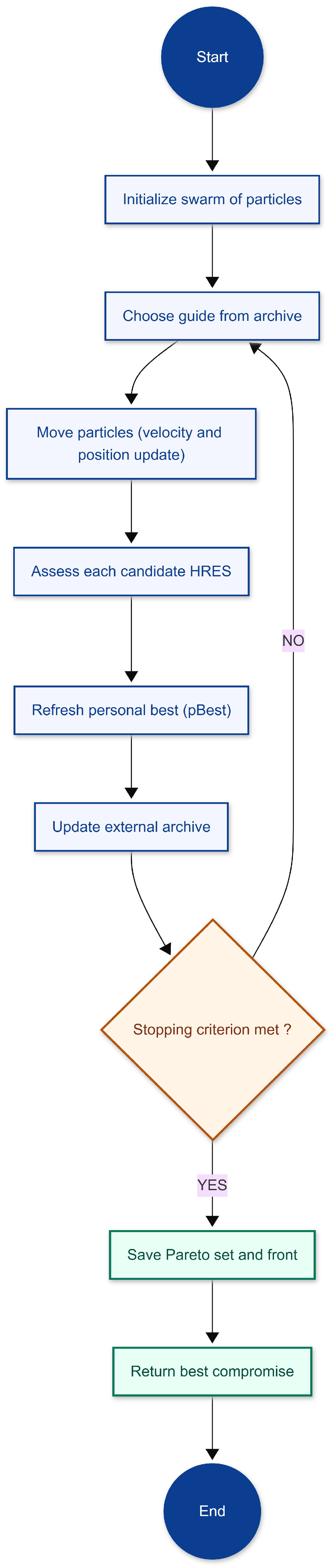
We employed MOPSO, as depicted in Figure 5, as a key comparison method. MOPSO is a powerful algorithm specifically designed to tackle complex multi-objective optimization problems.

Unlike standard PSO, it explicitly handles conflicting objectives, such as minimizing the LCOE, maximizing the REF, and minimizing the LPSP. It achieves this by utilizing a Pareto dominance mechanism and an external archive to store a diverse set of non-dominated solutions on the Pareto front [32,33].

MOPSO has a strong track record in real-world applications, from industrial optimization to the design of distributed energy systems. It is particularly effective at balancing exploration and exploitation, leading to rapid convergence towards high-quality solutions [32,34].

For this research, MOPSO models a complex decision space where each “particle” represents a unique technological configuration of the hybrid renewable energy system. These particles evolve through the decision space, guided by learning rules derived from their own history and the best archived solutions, with updates influenced by a leader selection mechanism.

This allows us to generate representative Pareto fronts, which are crucial for comparatively evaluating the DRL performance under various stress scenarios. Therefore, MOPSO serves as a robust reference method in this study, valued for the quality of its generated solutions and the diversity of the energy trade-offs that it identifies [32].

Table 7. MOPSO algorithm parameters.

Population Size	Iteration	Inertia Weight	Cognitive Coefficient	Social Coefficient
20	50	0.5	1.5	1.5

presents the values of the MOPSO parameters considered in this study [33,35].

2.5.4. Non-Dominated Sorted Genetic Algorithm II

The NSGA-II is a widely used, population-based, multi-objective evolutionary algorithm in the field of optimization due to its ability to produce well-distributed Pareto fronts while maintaining high-quality solutions efficiently [36,37,38,39].

The NSGA-II has been widely applied in sectors as varied as water management, energy architecture, and biological systems, with convincing results on the robustness and diversity of solutions [36].

Each individual in the population represents a specific microgrid technology configuration, comprising the number of PVs, the number of WTs, the BESS capacity, and the DG capacity. These individuals are assessed simultaneously according to three conflicting objectives: the LCOE, the LPSP, and the REF (Figure 6).

The NSGA-II employs an evolutionary process that includes selection, crossover, and mutation, followed by the classification of solutions based on their Pareto dominance and density metric, which preserves diversity without requiring partition parameters. Moreover, this approach includes a mechanism of elitism that merges the parental and child populations to ensure that the best solutions are maintained from one generation to the next [38,40].

The non-dominated sorting algorithm used in the NSGA-II exhibits an optimized computational complexity of $O\left({\mathrm{MN}}^2\right)$, where M represents the number of objectives and N denotes the population size. This enables the NSGA-II to efficiently identify reliable trade-offs between the economic, energy, and environmental performance in complex systems, such as HRESs. The NSGA-II is a relevant comparative method for assessing the quality of solutions generated by DRL-based approaches.

Table 8. NSGA-II algorithm parameters.

Population Size	Generation	Mutation Probability	Crossover Probability
20	50	0.1	0.9

presents the values of the NSGA-II parameters assumed in this study [41,42].

3. Results and Discussion

This section presents the sensitivity analysis results for the following different parameters: the load profile, system type, energy capacity via the generator, and grid. Additionally, it presents a comparative analysis of the DRL approach, MOPSO, and the NSGA-II regarding their ability to address the problem of sizing hybrid renewable energy systems.

3.1. Analysis of the Results of the DRL Approach

The analysis of the impacts of the parameters on the study’s parameters enables best practices to be defined during the HRES design process. When handled well, this step makes it possible to obtain an autonomous and resilient system.

3.1.1. Impacts of the Parameters on the LCOE

Figure 7 shows the impacts of the type of system, the load profile, the allowable rate via the generator, and the allowable rate via the public grid.

The analysis showed that systems with a higher share of renewable energy sources, such as PV + WT + BESS and PV + WT + BESS + DG, tend to exhibit a lower LCOE. The system becomes more profitable without a generator, scoring an average LCOE of around $0.3/kWh, likely due to its lower operating cost. However, the relatively large variability shows that the cost highly depends on other parameters such as $\tau$ and $\gamma$. Compared with the analysis on the profiles, we found that the best LCOE values were obtained in the following order: P1, P2, and P3. The P1 profile had a maximum LCOE below $0.4/kWh, regardless of the type of system. Profile 3, with a significantly higher LCOE, appeared to be a more difficult load to meet economically, probably due to the confidence intervals set for the PV, WT, BESS, and DG parameters.

An analysis of the allowable input, $\tau$, via the generator and the public grid, $\gamma$, showed that the system becomes profitable with high or low integration of the generator. This is probably due to overuse or underutilization, considering the initial costs. Meanwhile, grid access, that is, a high gamma, leads to a higher reliance on electricity purchases, which increases the average price. Conversely, network usage limitation, or a low $\gamma$, pushes DRL to optimize the local use of resources (PVs, WTs, and BESS), which is more economical.

3.1.2. Impacts of the Parameters on the LPSP

Figure 8 illustrates the impact of the four factors on the LPSP under the DRL method: the system type, load profile, generator threshold, and grid threshold.

The analysis of the system type revealed that the most complex hybrid architectures, such as PV + WT + BESS + DG, yielded the lowest LPSP values, approximately 0.25%. This confirms their reliability. Conversely, simple systems such as PV + BESS achieved very high LPSP levels, up to 0.70%, which reflects their inability to cover loads in specific scenarios. Thus, the diversity of energy production sources and the presence of storage are crucial to ensure continuous power. Compared with the effects of load profiles, the P3 profile exhibited the best performance, with an LPSP < 0.3%, unlike the P1 and P2 profiles. This performance may be due to better synchronization between the load profile and the available generation (PV/WT) or to the low variability in the profile.

The analysis of the effects of $\tau$ and $\gamma$ revealed that extreme $\tau$ values, such as 0.1 or 0.5, led to peaks in the LPSP, whereas intermediate values, around 0.2 to 0.3, resulted in a minimum LPSP. This result suggests that a $\tau$ that is too low limits the use of the generator, increasing the risk of a power failure. However, a $\tau$ that is too high could lead to an uncompensated additional cost. Compared with $\gamma$, the higher the $\gamma$, the lower the LPSP. At a $\gamma$ greater than or equal to 0.3, the LPSP drops to less than 0.3%, indicating a strong dependence on network access, which makes it possible to avoid failures.

3.1.3. Impacts of Parameters on the REF

The REF, an indicator of the share of energy produced by renewable sources (PV, WT) in relation to demand, states that a high REF is desirable because it indicates a more economic system and less dependence on fossil fuels or the grid.

Figure 9 analyzes the impact of the different study parameters on the REF in the DRL configurations: the type of system, load profile, $\tau$, and $\gamma$.

The analysis showed that the PV + WT + BESS + DG and PV + WT + BESS hybrid systems had high REFs, around 65% to 70%. On the other hand, configurations without wind turbines, such as PV + BESS + DG and PV + BESS, had a lower REF, sometimes less than 35%. However, the significant variability in the graph indicates that other parameters, such as energy profiles or constraints, may also impact the REF. Thus, introducing wind power plays a key role in increasing the rate of renewable energy in HRESs. Comparatively, the analysis following the profiles showed a better temporal correlation between renewable generation and demand in Profile 3. Thus, the load profile influences the system’s ability to exploit renewable energy sources. The profile variability defines the compatibility with intermittent resources.

The effects of $\tau$ and $\gamma$ on the REF are apparent. The REF increased sharply for average values of $\tau$, around 0.2 to 0.3, reaching a peak above 90%, and then decreased beyond that for tau values above 0.4. Thus, the moderate use of the generator enables DRL to favor the exploitation of renewable energy sources. A $\tau$ that is too high outbids fossil production, reducing the renewable share. Regarding the $\gamma$ impact, the REF reached its peak with approximately 90% of $\gamma$, equivalent to 0.3. The relationship between $\gamma$ and the REF is nonlinear. An intermediate value can maximize the synergies between renewable resources and network access. Although it may seem counterintuitive, a higher $\gamma$ can sometimes force the DRL agent to preserve renewable resources for local autonomy. This encourages smart trade-offs, i.e., strategic compromises between cost, reliability, and sustainability.

3.2. DRL, MOPSO, and NSGA-II Comparison

This section presents a comparative analysis of the different methods in relation to the study’s objectives, specifically the LCOE, the REF, and the LPSP.

The following subsections present the values computed in the present study; to facilitate comparison across scenarios, we maintain a heatmap visualization layout consistent with our earlier work [18].

3.2.1. Comparison of Methods According to the LCOE

The heatmap in Figure 10 summarizes the average LCOE obtained by the three methods—DRL, MOPSO, and the NSGA-II—across the three load profiles of the study.

The DRL method achieved the best LCOE values for the P1 and P2 profiles, with $0.35/kWh and $0.44/kWh, respectively. In comparison, the MOPSO method yielded $0.37/kWh for P1 and $0.45/kWh for P2, while the NSGA-II produced $0.37/kWh for P1 and $0.47/kWh for P2. Thus, all algorithms presented good results with a low dispersion on the P1 and P2 profiles. However, the algorithms showed an increase in the LCOE on the P3 profile, which could indicate that the P3 profile does not lend itself well to the study context, probably due to its sensitivity to learning parameters or system dynamics. Beyond the numerical ranking, this comparison suggests that DRL is particularly effective when the design problem requires adaptive coordination between component sizing and constrained backup usage. Its advantage on P1 and P2 indicates that sequential learning helps identify economically favorable compromises when the demand structure remains compatible with the available renewable resources. In contrast, the degradation observed on P3 suggests a more difficult economic landscape in which renewable-load matching is weaker or backup margins are more restrictive relative to the profile characteristics.

3.2.2. Comparison of Methods According to the LPSP

Figure 11 presents a comparative analysis of the DRL, MOPSO, and NSGA-II methods based on the LPSP objective function.

The analysis shows that all methods had an average LPSP value of approximately 0.5%, which testifies to their ability to provide relatively reliable systems. The economic trade-offs of the approach can explain the high DRL values compared with the other objectives. However, it is essential to note that MOPSO and NSGA-II offer the best reliability on all three profiles. Thus, while DRL provides a flexible approach, it can be hindered by suboptimal exploration in specific scenarios. This is itself an important result: the proposed DRL framework should not be interpreted as universally superior on every criterion, but rather as a flexible optimizer capable of favoring broader trade-offs. When reliability is prioritized in a strongly conservative sense, the evolutionary baselines remain competitive; when a broader compromise involving cost and renewable penetration is sought, DRL becomes more attractive.

3.2.3. Comparison of Methods According to REF

The analysis of Figure 12 presents a comparative study of the different methods according to the REF, showing that DRL performed poorly for Profile 1, probably due to strategic choices aimed at other trade-offs.

In Profile 2, DRL demonstrated a good compromise between renewable autonomy and the economic performance of the system. An analysis of Profile 3 showed that DRL achieved a better score of around 73%, compared with only 21% for MOPSO and NSGA-II. This result highlights DRL’s adaptive learning capacity, which gives it a decisive superiority in complex and dynamic environments compared with the MOPSO and NSGA-II methods. The gain in the REF should therefore be interpreted as a structural advantage in renewable prioritization rather than as a simple numerical improvement. In the most constrained profile, policy-based learning appears better able to exploit non-obvious renewable-oriented strategies while still respecting backup-energy limits.

From a computational perspective, the three compared methods differ in nature. DRL incurs an upfront training cost because candidate decisions are evaluated repeatedly through interaction with the environment and replay-based updates. In return, it learns a policy that can guide future decisions in a structured manner. In contrast, MOPSO and NSGA-II are population-based optimizers whose computational effort is mainly driven by the number of candidate solutions evaluated per iteration or generation. In the present study, the MOPSO and NSGA-II were configured with a population size of 20 and 50 iterations/generations, which provides a controlled benchmark setting. Moreover, the NSGA-II includes a non-dominated sorting stage with complexity $O\left(M{N}^2\right)$, where M is the number of objectives and N is the population size. The improved REF performance obtained by DRL should therefore not be interpreted as being cost-free; rather, it reflects a different allocation of computational effort, where more learning is performed during optimization in exchange for a greater adaptive capacity in complex trade-off regions.

It is also important to note that the present study was simulation-based. Although the analysis relied on real load-profile sources and representative TMY climatic data, it did not include field deployment or hardware-in-the-loop validation. Accordingly, the contributions of this research should be interpreted as methodological and comparative, with real-system validation constituting a logical next step for future work.

4. Conclusions

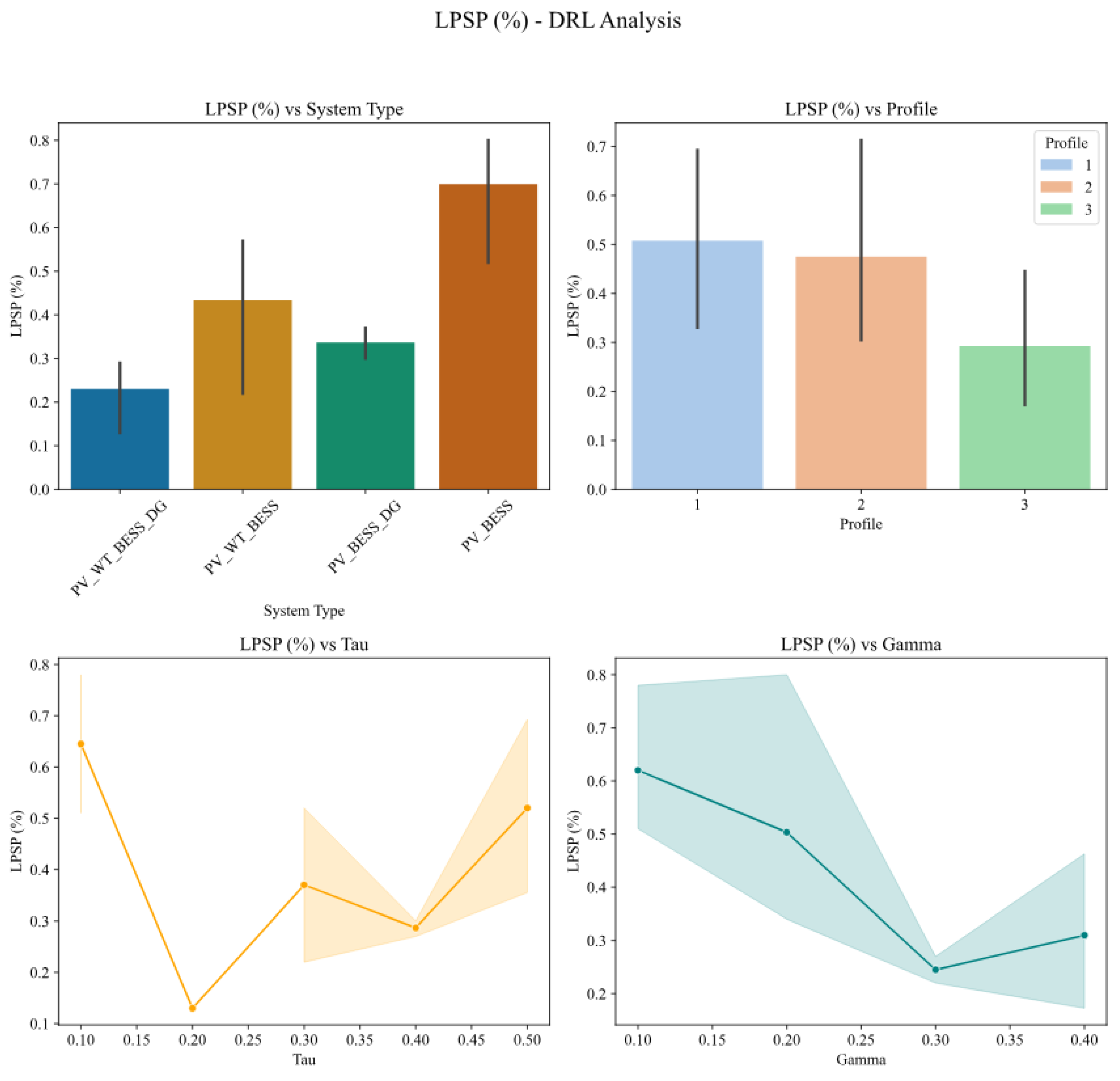
This study presents a sensitivity analysis framework for HRES sizing in which tau and gamma are treated as explicit admissible backup-energy ratios for the generator and the grid. The analysis was conducted across four HRES configurations and three contrasting load profiles with the objective of understanding how these constraints reshape the compromise between three conflicting criteria: the LCOE, LPSP, and REF.

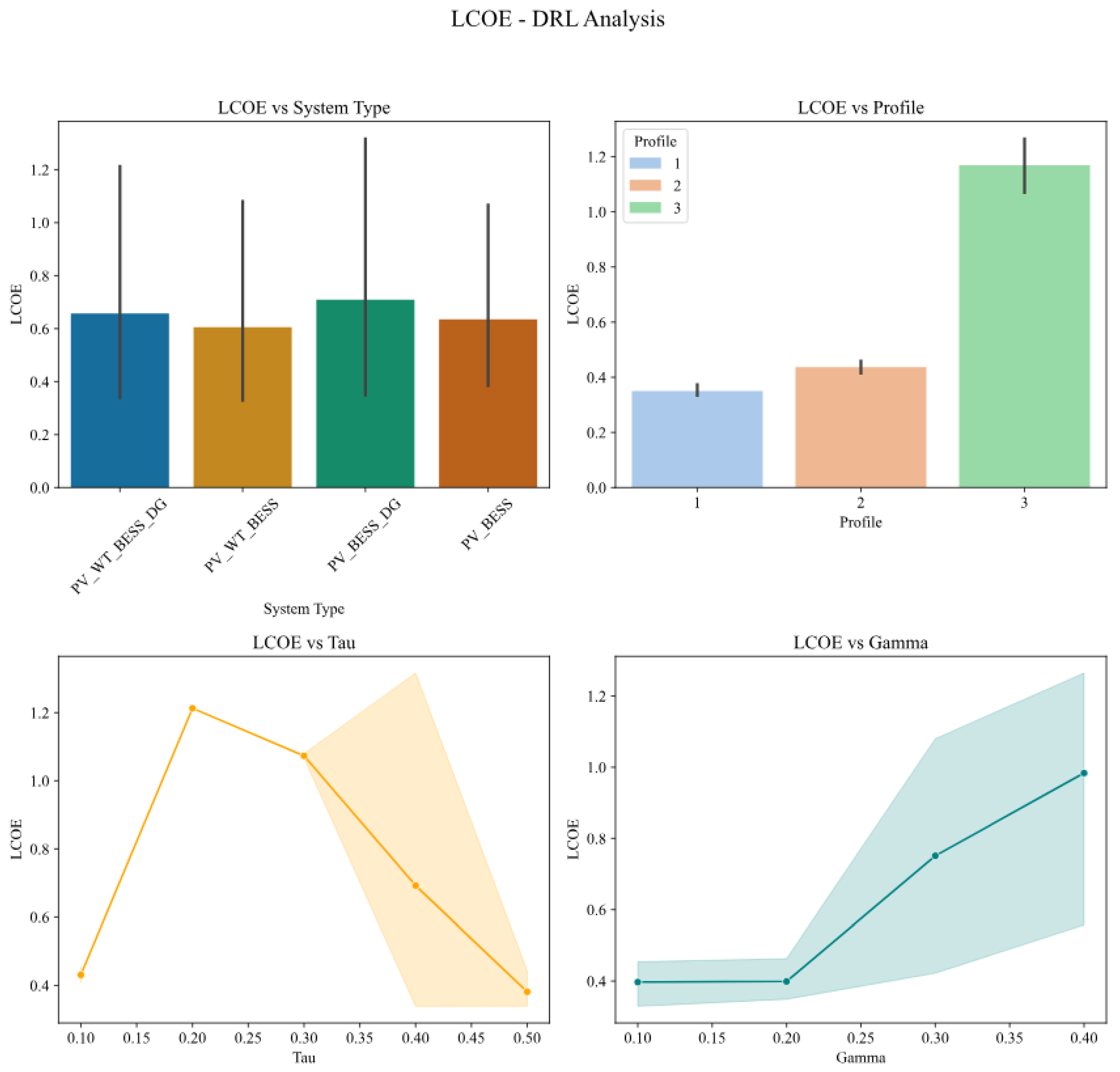
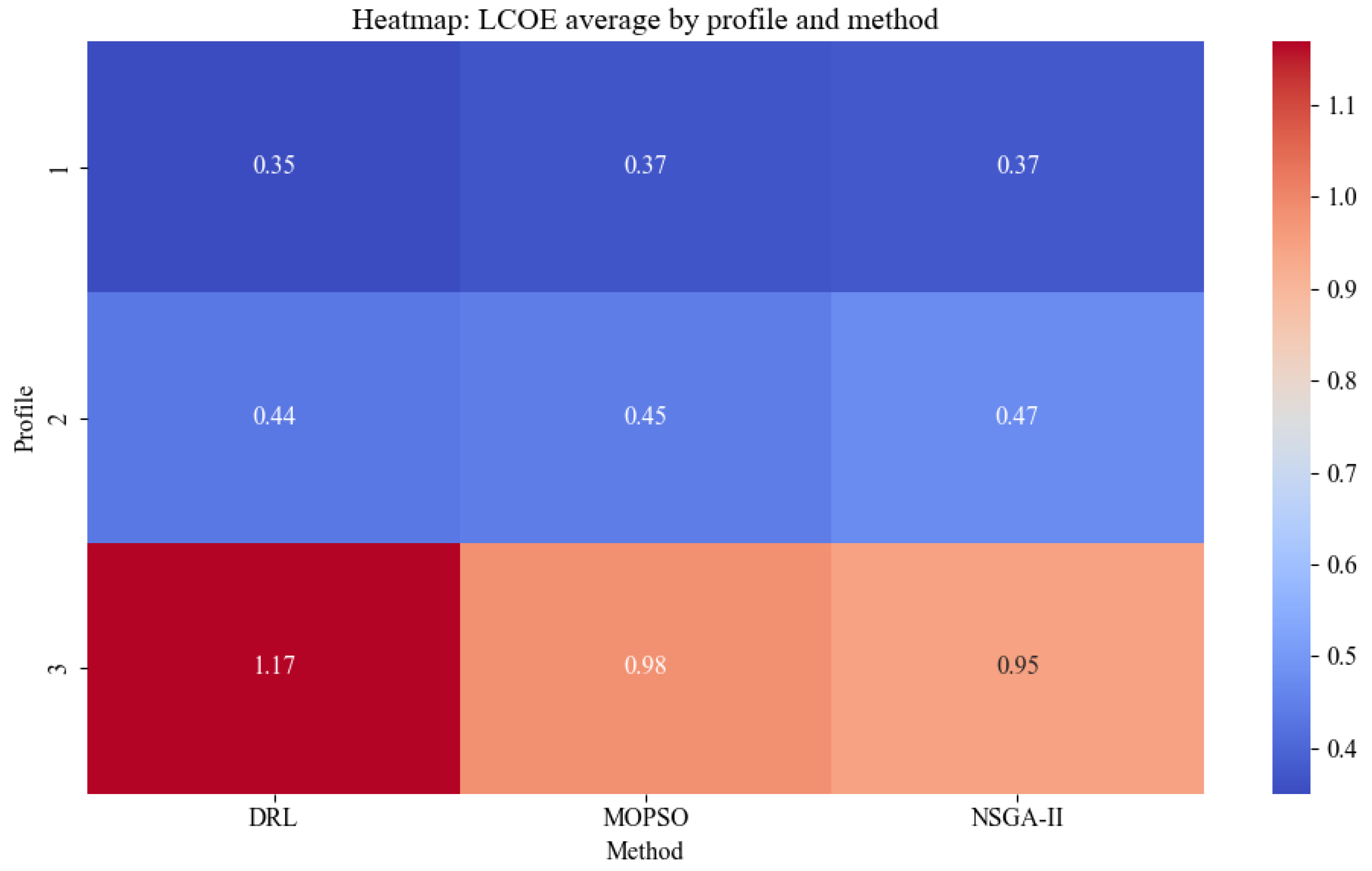
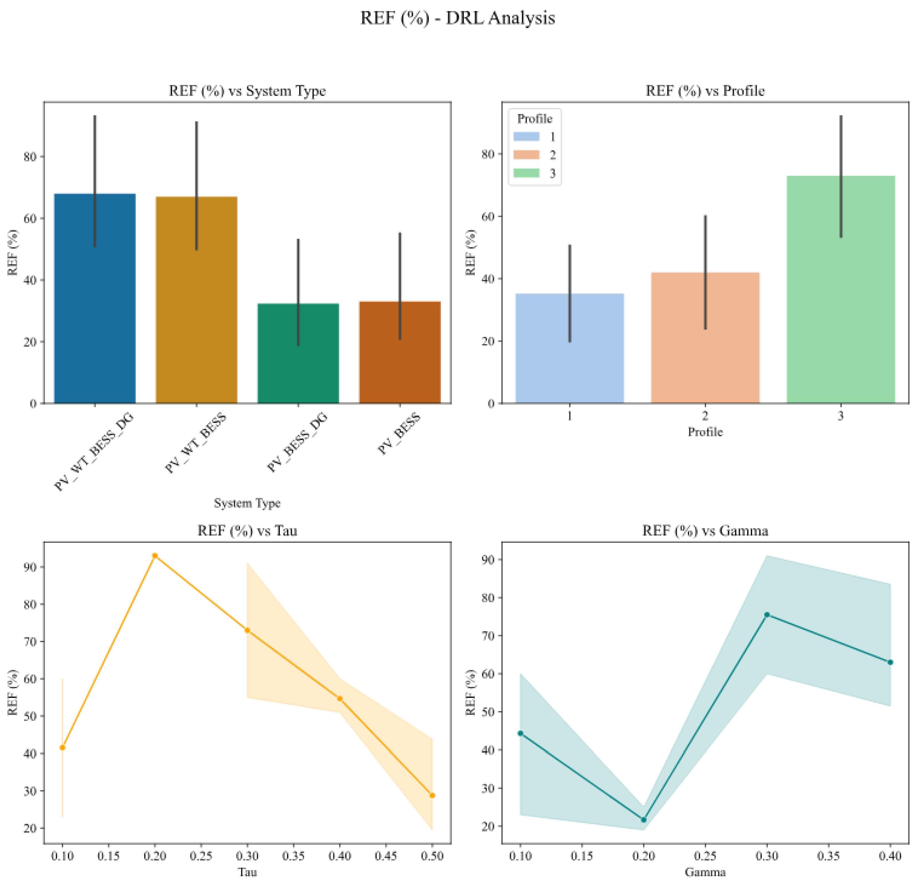
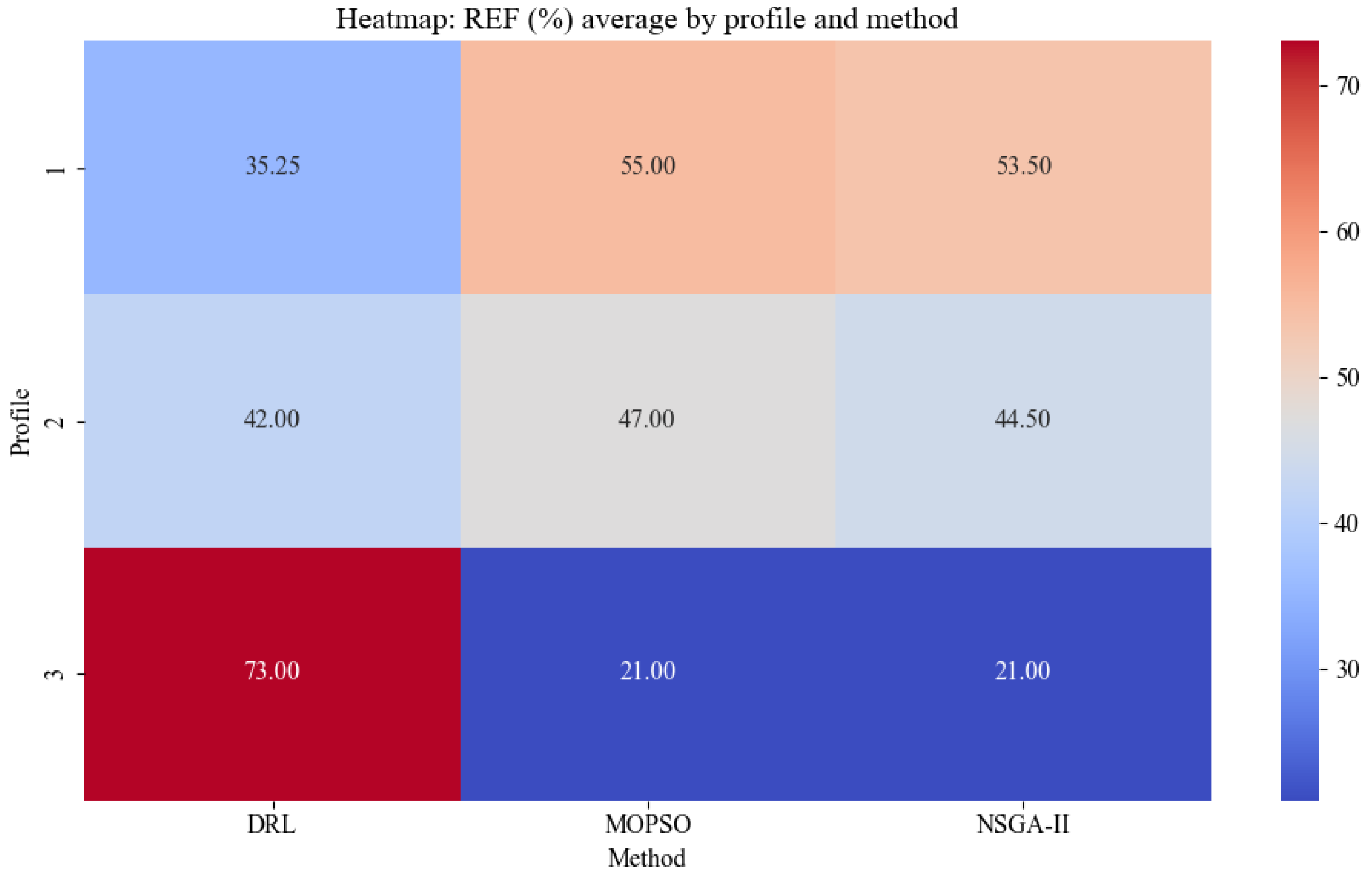
The experimental results show that the main value of the proposed DRL approach lies not in universal dominance, but in its ability to uncover adaptive trade-offs in complex scenarios, especially when the demand variability and production structure are more difficult to control. The analyses revealed that various factors impact the sizing process of hybrid renewable energy systems. First, the results show that the type of system plays a central role in the overall performance. Configurations that integrate multiple sources, including PV panels, WTs, a BESS, and a DG, offer the best trade-off between the LCOE, LPSP, and REF. Specifically, for a PV + WT + BESS + DG system, the DRL approach can identify parameters that ensure a robust system performance, achieving a low LPSP (below 0.3%) and a competitive LCOE (under $0.4/kWh). Compared with MOPSO and NSGA-II, DRL also maintains a high REF exceeding 60%.

Dimensioning also requires that the technical constraints be carefully calibrated. A value that is too low (<0.1) limits the generator’s backup supply, increasing the LPSP, while a value that is too high (>0.4) penalizes the REF and increases the LCOE. The results suggest that an average $\tau$ (∼0.25–0.3) allows the DRL method to use the generator only when economically and ecologically justified. As for $\gamma$, an intermediate level (∼0.3) seems more suitable. This intermediate value provides sufficient flexibility without inducing excessive dependence on the grid. This approach maximizes the return on investments while controlling costs.

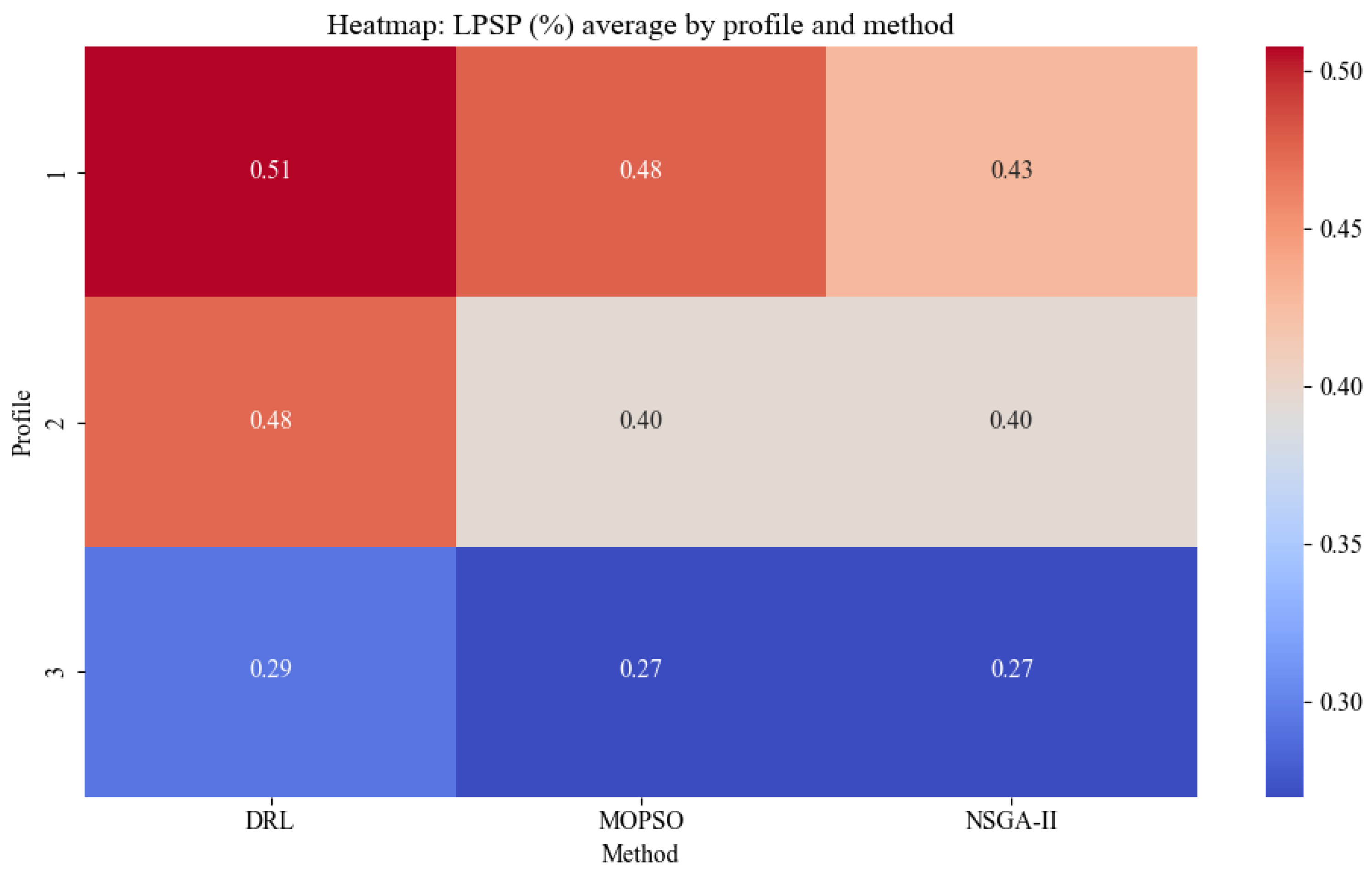
Compared with the MOPSO and NSGA-II methods, the results also show that the adopted DRL approach can adapt to changing multi-objective constraints, even if the LPSP or LCOE performance remains more dispersed in some contexts, depending on the specific conditions. In contrast, MOPSO and NSGA-II offered greater stability and reliability in standard scenarios, at the cost of less use of renewable sources.

Through these analyses, this study suggests utilizing DRL in dynamic contexts, where the objective is to enhance energy autonomy and integrate renewable energies while maintaining strategic adaptability to operational constraints. Thus, a hybrid combination with more conservative methods can be considered for systems subjected to strict requirements for the continuity of supply.

Overall, the results suggest that intermediate admissible backup thresholds offer better compromises than extreme values. Moderate tau and gamma values provide enough operational flexibility to preserve reliability without inducing excessive dependence on fossil-based or grid-supplied energy. In that sense, the framework provides design-oriented guidance for resilient and low-carbon HRES planning.

As a result, the following avenues of research for improving the DRL approach are presented:

• Hybridization of the DRL method with conservative approaches to improve the accuracy between exploration and exploitation.
• Adaptation of the DRL to dynamic electricity markets.
• Coupling the DRL with weather and load forecasts for long-term predictive optimization.

In short, by strengthening the robustness of the DRL, it could position itself as a technological pillar of the smart energy transition.