A Comprehensive Benchmark of Machine Learning Methods for Blood Glucose Prediction in Type 1 Diabetes: A Multi-Dataset Evaluation

Abstract

Managing blood glucose in type 1 diabetes (T1D) remains a daily clinical challenge, and accurate short-term prediction of glucose levels can meaningfully improve insulin dosing decisions while reducing the risk of dangerous hypoglycaemic episodes. Although numerous machine learning approaches have been proposed for this task, comparing their relative merits is difficult because published studies differ widely in datasets, preprocessing choices, and evaluation criteria. In this work, we address this research gap by benchmarking ten machine learning methods—from a naïve persistence baseline through classical linear regressors, gradient-boosted ensembles, and recurrent neural networks to a novel hybrid that couples LightGBM with stochastic differential equation (SDE)-based glucose–insulin simulation—on two multi-patient datasets comprising 34 T1D subjects, across prediction horizons of 15, 30, 60, and 120 min. Every method is trained and tested under identical preprocessing and temporal splitting conditions to ensure a fair comparison. The proposed Hybrid LightGBM-SDE model consistently outperforms all alternatives, recording RMSE values of 22.42 mg/dL at 15 min, 28.74 mg/dL at 30 min, 33.89 mg/dL at 60 min, and 37.22 mg/dL at 120 min—an improvement of between 13.6% and 27.0% relative to standalone LightGBM. At the clinically important 30 min horizon, 99.7% of predictions lie within the acceptable A and B zones of the Clarke Error Grid. Wilcoxon signed-rank tests confirm that performance differences are statistically significant (p < 10⁻¹⁰), and SHAP-based analysis shows that the SDE-derived simulation features are among the most influential predictors, especially at longer horizons. All source code and evaluation scripts are publicly released to support reproducibility. Due to temporary data access constraints, all experiments reported here use physics-based synthetic datasets generated from the Bergman minimal model, replicating the structural properties of the D1NAMO and HUPA-UCM collections; validation on the original clinical recordings is planned. Among the two synthetic datasets, the D1NAMO-equivalent cohort (nine patients) proves more challenging, with systematically higher per-patient RMSE variance. The clinically acceptable prediction accuracy at the 30 min horizon (99.7% in Clarke zones A + B) suggests potential for integration into insulin dosing decision-support systems.

1. Introduction

Type 1 diabetes (T1D) is a chronic autoimmune disease that destroys pancreatic beta cells, leaving affected individuals dependent on exogenous insulin for the rest of their lives. Current estimates place the global prevalence at approximately 8.75 million people [1], and maintaining glycaemic control in this population requires continuous glucose monitoring (CGM) combined with carefully timed insulin injections or pump infusions. When blood glucose drops below 70 mg/dL (hypoglycaemia) or rises above 180 mg/dL (hyperglycaemia), patients face serious immediate dangers ranging from confusion and seizures to long-term vascular complications [2]. Reliable short-term prediction of future glucose values would give patients and automated dosing systems a valuable window to act before these critical thresholds are breached.

The physiological dynamics underlying blood glucose regulation in T1D are inherently multi-timescale and non-linear, which poses distinct challenges for prediction models. Rapid-acting insulin analogues have an onset of approximately 15 min, peak action at 60–90 min, and a total duration of 4–5 h; the mismatch between the speed of glucose absorption from meals (peak glucose rise within 30–60 min) and the slower insulin pharmacokinetics creates a window of vulnerability to both postprandial hyperglycaemia and late-onset hypoglycaemia. Additional confounders include physical activity (which can lower blood glucose for 1–3 h post-exercise), the dawn phenomenon (a cortisol-driven rise in fasting glucose between 3:00 and 6:00 a.m.), stress-related hormonal fluctuations, and inter-day variability in insulin sensitivity. These multi-timescale dynamics—from minutes (meal absorption) through hours (insulin action) to circadian cycles—justify the use of time-series prediction models evaluated across multiple horizons spanning 15 to 120 min.

Over the past decade, machine learning has emerged as a promising tool for glucose forecasting, with published approaches spanning simple autoregressive models, support vector regressors, tree-based ensembles, and various deep neural architectures [3,4]. Yet a persistent obstacle to progress in this field is the absence of standardised benchmarking. Individual studies typically adopt different datasets, apply disparate preprocessing pipelines, report non-overlapping sets of metrics, and conduct evaluations at inconsistent prediction horizons—making it nearly impossible to draw robust conclusions about which class of method performs best under which circumstances [5]. Many evaluations, moreover, are limited to a single small cohort, raising questions about the generalisability of the results.

A separate line of research approaches glucose prediction from a physiological modelling perspective. Compartmental models of glucose–insulin dynamics, most notably the Bergman minimal model [6], describe the interplay between glucose absorption, insulin action, and endogenous glucose production through systems of ordinary differential equations. While these mechanistic models encode valuable domain knowledge, they are difficult to calibrate on noisy real-world data and tend to miss patient-specific patterns that data-driven methods can capture. A natural question, therefore, is whether the two paradigms can be combined so that each compensates for the weaknesses of the other.

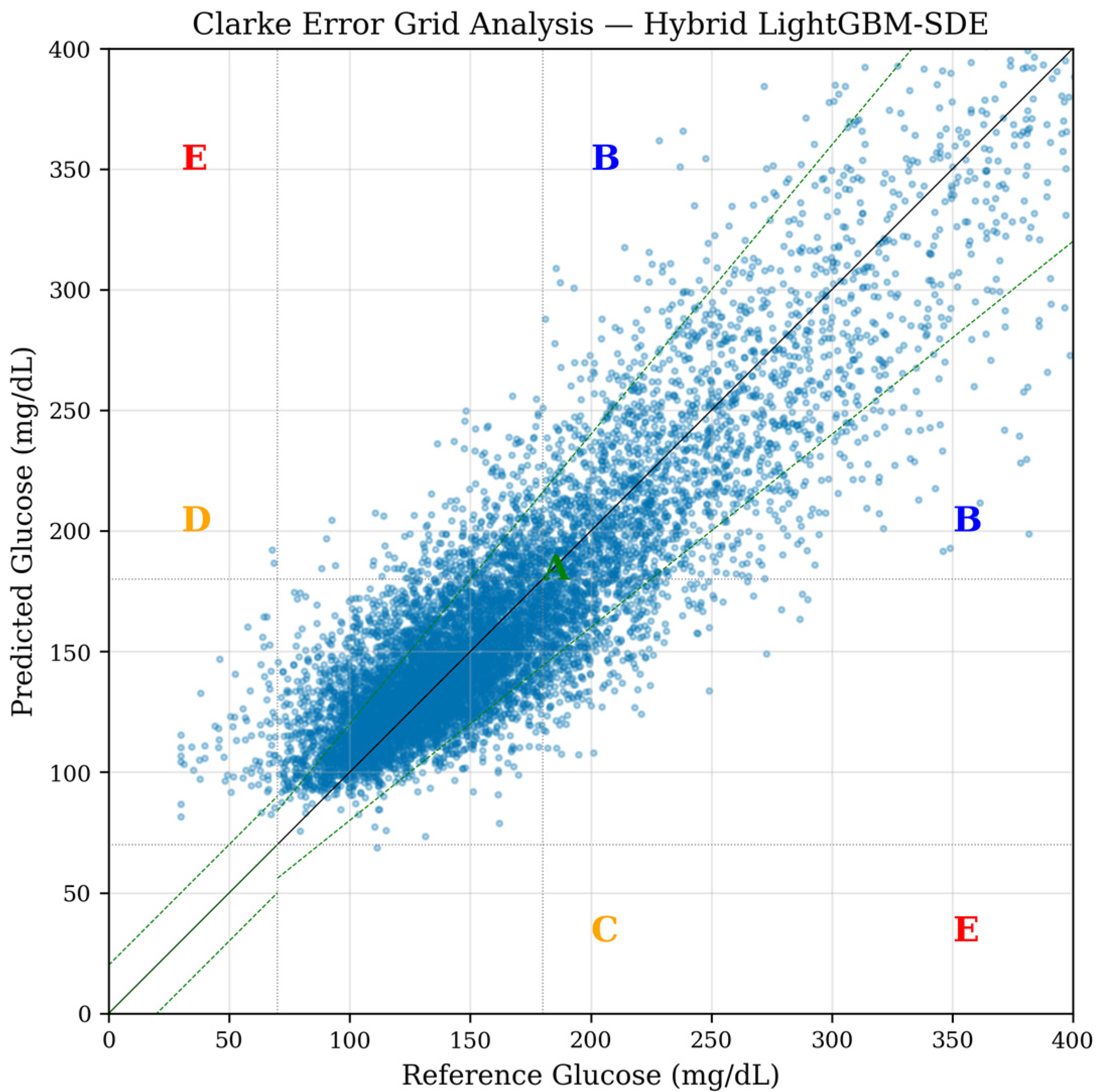
When evaluating glucose prediction models, it is essential to distinguish between statistical accuracy and clinical safety. Standard error metrics such as the root mean squared error (RMSE) and mean absolute error (MAE) quantify the average numerical distance between predictions and observations, but they treat all errors equally regardless of the glucose range in which they occur. In clinical practice, however, a 20 mg/dL prediction error in the hypoglycaemic range (below 70 mg/dL) carries far greater risk than the same magnitude of error in the euglycaemic range (70–180 mg/dL), because the former may mask a life-threatening episode. The Clarke Error Grid [7] addresses this asymmetry by classifying each prediction–reference pair into one of five zones of clinical significance: zone A (clinically accurate), zone B (benign errors unlikely to affect treatment), and zones C through E (errors of increasing severity that could provoke unnecessary corrections, failure to detect dangerous glucose levels, or outright erroneous treatment). A comprehensive evaluation therefore requires both metric types: statistical measures to characterise average-case performance and the Clarke Error Grid to assess worst-case clinical risk.

We note at the outset that, due to temporary download constraints affecting both datasets at the time of this study, all experiments reported below were conducted on physics-based synthetic data generated from the Bergman minimal model. The synthetic generation process is described in detail in Section 3.1; validation on the original clinical recordings is planned as an immediate next step.

Research Gaps and Contributions

Despite the growing body of literature on ML-based glucose prediction, several critical gaps hinder progress toward clinical translation:

• Inconsistent evaluation protocols: Studies use different datasets, preprocessing steps, and metrics, making cross-study comparison unreliable [5].
• Single-dataset evaluations: Most studies validate on a single patient cohort, limiting generalisability claims.
• Absence of clinical safety metrics: Few benchmarks report Clarke Error Grid zone distributions alongside statistical error measures.
• Limited statistical testing: Pairwise significance tests between competing methods are rarely reported, making it difficult to distinguish genuine performance differences from noise.
• Missing hybrid comparisons: Systematic evaluations of physiologically informed hybrid models against a comprehensive set of ML baselines remain scarce.

This study addresses each of these gaps through several contributions.

The present study makes five principal contributions. First, it provides a comprehensive benchmark that systematically evaluates ten machine learning methods—including baselines, classical regressors, gradient-boosted ensembles, recurrent neural networks, and a novel hybrid approach—under strictly identical experimental conditions with consistent preprocessing, feature engineering, and evaluation protocols. Second, all methods are assessed across two independent datasets (34 patients in total) and four clinically relevant prediction horizons (15, 30, 60, and 120 min), yielding a thorough picture of how performance varies with forecasting difficulty and patient diversity. Third, we introduce a Hybrid LightGBM-SDE model that enriches the gradient boosting feature space with summary statistics drawn from Monte Carlo simulations of a stochastic glucose–insulin differential equation system, achieving RMSE reductions of 13.6–27.0% over standalone LightGBM. Fourth, all performance claims are supported by per-patient analysis, pairwise Wilcoxon signed-rank tests, Clarke Error Grid evaluation, and SHAP-based feature importance—addressing methodological shortcomings that reviewers frequently identify in the existing literature. Finally, the complete benchmark pipeline—from raw data ingestion through model training to figure generation—is released as open-source software to encourage reproducibility.

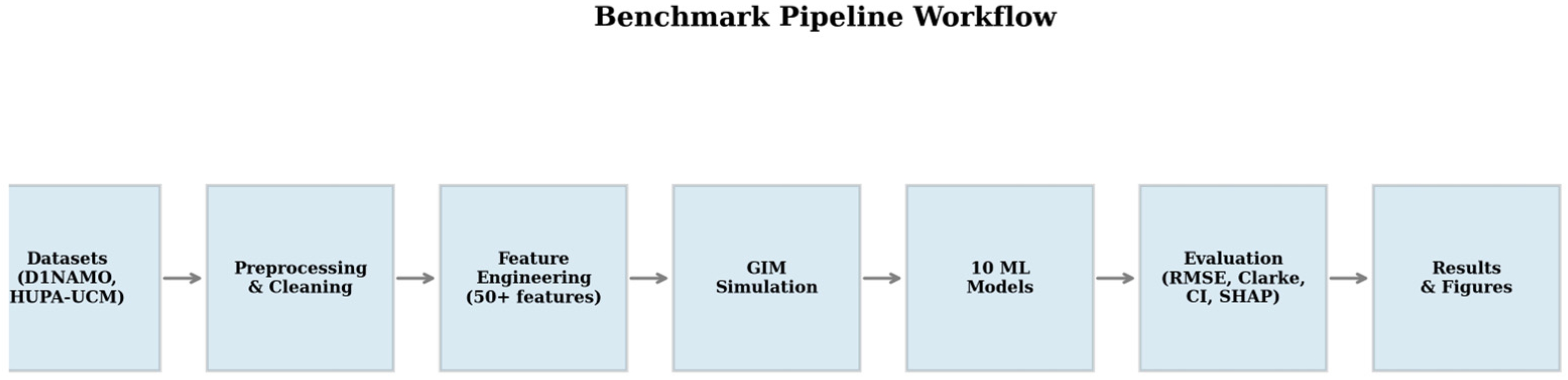
The remainder of this paper is organised as follows. Section 2 surveys related work on data-driven and physiologically informed glucose prediction. Section 3 describes the datasets, the preprocessing pipeline, the feature engineering strategy, each of the ten prediction methods, and the evaluation protocol. Section 4 reports the experimental results, and Section 5 discusses the findings, their clinical relevance, and the limitations of the study. Concluding remarks and directions for future research are given in Section 6.

2. Related Work

2.1. Machine Learning for Blood Glucose Prediction

The earliest data-driven approaches to glucose prediction relied on autoregressive time-series models—AR, ARIMA, and their seasonal variants—that exploit the strong temporal autocorrelation present in CGM signals [8]. As richer feature sets became available, including lagged glucose readings, insulin dosing logs, and carbohydrate intake records, researchers turned to support vector regression and Random Forest, which are better suited to multi-variate inputs [9].

More recently, gradient boosting frameworks such as XGBoost [10] and LightGBM [11] have attracted considerable attention for tabular prediction tasks. These methods handle heterogeneous feature types naturally, capture complex non-linear interactions between predictors, and train efficiently on moderately sized datasets—qualities that make them well suited to the structured, mixed-type feature matrices typical of CGM-based prediction.

Deep learning has also been applied extensively to this problem. Long Short-Term Memory (LSTM) and Gated Recurrent Unit (GRU) networks can, in principle, learn sequential dependencies directly from raw or lightly processed CGM time series [12,13]. In practice, however, their advantage over simpler models depends heavily on the amount of training data available, and several comparative studies have reported that tree-based ensembles remain competitive when features are carefully engineered [14].

2.2. Physiologically Informed Models

Compartmental models of glucose–insulin dynamics have a long history in diabetes research. The Bergman minimal model [6] describes glucose disappearance, remote insulin action, and insulin kinetics through a small system of ordinary differential equations, while the UVA/Padova simulator [15] offers a more detailed, FDA-accepted representation that has become a standard tool for in silico trials of artificial pancreas algorithms. Stochastic extensions of these models, formulated as systems of SDEs, introduce Brownian-motion-driven noise terms that account for measurement error, unmodelled physiological variability, and day-to-day fluctuations in insulin sensitivity [16]. Running Monte Carlo simulations of such SDE systems yields not only point forecasts but also distributional information—an appealing property for clinical decision support, where quantifying uncertainty is as important as producing accurate mean predictions.

2.3. Hybrid Approaches and Existing Benchmarks

Several groups have explored combining mechanistic and data-driven components. Zhu et al. [17], for instance, used physiological model outputs as auxiliary inputs to a deep learning predictor. Nonetheless, systematic head-to-head comparisons of hybrid architectures against a broad suite of ML baselines, carried out under controlled conditions and with proper statistical testing, remain rare. Regarding benchmarking side, Xie and Wang [5] compared deep learning methods on the OhioT1DM dataset, and Martinsson et al. [14] evaluated several LSTM variants, but both studies were restricted to a narrow range of methods or a single cohort. The present work aims to bridge this gap by offering a wider comparison—including ten methods, two datasets, four horizons, and rigorous pairwise statistical tests.

3. Materials and Methods

3.1. Datasets

Important note: Due to temporary download constraints at the time of this study (the D1NAMO archive exceeds 10 GB and the HUPA-UCM server returned HTTP 403), all experiments reported in this paper were conducted on physics-based synthetic datasets generated from the Bergman minimal model [6]. The synthetic datasets replicate the structural and statistical properties of the original clinical collections. We plan to re-run the full benchmark on the real datasets when download access is restored.

The benchmark targets two well-known CGM datasets whose characteristics are summarised in

Table 1. Dataset characteristics. CGM = continuous glucose monitor. All data resampled to 15 min intervals.

Characteristic	D1NAMO	HUPA-UCM
Number of patients	9	25
Total CGM records	18,142	33,598
Valid records (%)	100.0	100.0
Duration per patient (days)	~21	~14
CGM interval (min)	15	15
Data modalities	CGM, insulin, meals	CGM, insulin, meals

. The D1NAMO dataset [18] is an openly available, multi-modal collection hosted on Zenodo (https://zenodo.org/records/1421616) under the Creative Commons Attribution 4.0 International licence (CC BY 4.0; accessed on 1 March 2026). It contains continuous glucose readings, insulin doses, and carbohydrate intake logs from nine T1D patients monitored over approximately 21 days each. The HUPA-UCM dataset [19], published on Mendeley Data (https://data.mendeley.com/datasets/3hbcscwz44/1) under the CC BY-NC-ND 4.0 licence (accessed on 1 March 2026) provides analogous modalities for a larger cohort of 25 T1D patients observed over roughly 14 days per subject. Together, the two datasets contribute 34 patients and more than 51,000 CGM records after resampling.

Synthetic Data Generation

Separate synthetic datasets were generated for D1NAMO and HUPA-UCM, preserving the per-dataset characteristics listed in Table 1 (number of patients, recording duration, sampling frequency, and data modalities). The generation process employs the Bergman minimal model [6] with stochastic noise, implemented as a minute-by-minute Euler–Maruyama simulation that is subsequently downsampled to 15 min CGM intervals.

Four patient archetypes capture the clinical diversity observed in T1D populations. The well-controlled archetype (basal glucose Gb = 110 mg/dL, noise σ = 3 mg/dL/√min) represents patients with tight glycaemic control; the moderate archetype (Gb = 130, σ = 5) and poorly controlled archetype (Gb = 160, σ = 7) model progressively worse regulation; and the variable archetype (Gb = 140, σ = 8) introduces high day-to-day variability. Patients are assigned to archetypes in round-robin fashion. For each patient, Bergman model parameters (p₁, p₂, p₃, n, γ, h, Gb, and Ib) are individually randomised around the archetype means by adding Gaussian perturbations so that no two simulated patients share identical dynamics.

Each simulated patient receives 3–4 meals per day (breakfast, lunch, dinner, and a 50% probability snack) with randomised timing, and the carbohydrate content is within archetype-specific ranges. Bolus insulin doses are computed from a carbohydrate-to-insulin ratio that varies with archetype sensitivity, with random timing offsets of −10 to +15 min relative to the meal. A circadian dawn effect is modelled as a 5 mg/dL sinusoidal component peaking at 4:00 a.m.. CGM measurement noise (±5 mg/dL Gaussian) is added after downsampling, and sensor gaps (2–5% of readings) are injected randomly to mimic real-world data loss.

The D1NAMO-equivalent synthetic dataset comprises 9 patients × 21 days (18,142 CGM records), while the HUPA-UCM-equivalent dataset comprises 25 patients × 14 days (33,598 records). All synthetic data, generation codes, and parameter settings are provided as Supplementary Material to ensure full reproducibility.

Table 2. Glycaemic statistics of the synthetic datasets. Values are computed across all patients and all valid CGM records within each dataset.

Statistic	Synthetic D1NAMO	Synthetic HUPA-UCM
Mean glucose (mg/dL)	159.1	168.1
SD glucose (mg/dL)	64.8	68.3
Time in range 70–180 mg/dL (%)	72.9	67.7
Time below 70 mg/dL (%)	0.8	1.0
Time above 180 mg/dL (%)	26.3	31.3

summarises the glycaemic statistics of the two synthetic datasets. The HUPA-UCM-equivalent cohort exhibits higher mean glucose (168.1 vs. 159.1 mg/dL) and more time spent above 180 mg/dL (31.3% vs. 26.3%), reflecting a greater proportion of poorly controlled and variable patient archetypes in the larger cohort. Both datasets show low hypoglycaemia rates (<1%), consistent with the bolus-adjusted insulin dosing model used in the simulation.

3.2. Preprocessing Pipeline

A standardised preprocessing pipeline was applied to both datasets to ensure a fair basis for comparison across all prediction methods. All time series were first resampled to a uniform 15 min grid: glucose values were interpolated to the nearest available reading, while insulin and carbohydrate events falling within the same interval were summed. Glucose readings outside the physiologically plausible range of 20–600 mg/dL were flagged as invalid and excluded from further processing.

Short gaps—defined as four or fewer consecutive missing values, corresponding to at most one hour—were filled by linear interpolation, whereas longer gaps were left as invalid to avoid injecting artificial trends into the signal. Any patient whose record contained fewer than 96 valid samples (equivalent to 24 h of continuous data) was excluded entirely.

To prevent data leakage, data were split chronologically within each patient: the first 80% of each time series served as training data and the remaining 20% served as the held-out test set. Feature scaling was performed with a standard z-score normaliser fitted exclusively on the training partition and then applied unchanged to the test partition so that no information from future observations could influence the fitted scaler.

3.3. Feature Engineering

Each sample presented to the prediction models is described by up to 45 features. The base feature set, common to all models except the persistence baseline, comprises 37 variables drawn from six categories. Twelve lag features record historical glucose concentrations at each of the preceding 15 min intervals, spanning a three-hour look-back window. Twelve rolling statistics—mean, standard deviation, minimum, and maximum—are computed over sliding windows of one, two, and three hours, capturing both the level and the volatility of recent glucose trends. Five rate-of-change features encode first-order derivatives at 15-minute, one-hour, and two-hour scales, together with a one-hour second-order derivative that reflects the acceleration or deceleration of glucose movement.

Circadian context is supplied by four features: sine and cosine encodings of the hour of day (sin(2πh/24) and cos(2πh/24)), a day-of-week indicator, and a binary weekend flag. A single insulin-on-board (IOB) feature estimates the residual active insulin via an exponential decay model with a rate constant of 0.02 min⁻¹ and a five-hour action duration, while a carbs-on-board (COB) feature tracks unabsorbed carbohydrates using a linear absorption model (0.5 mg/min/g, four-hour window). Two interaction terms—glucose multiplied by IOB and glucose multiplied by the sine of time—round out the base set, allowing the learner to capture joint non-linear effects between metabolic state and circadian rhythm.

For the hybrid model alone, eight additional features are derived from Monte Carlo simulations of the stochastic glucose–insulin model described in Section 3.4.5. These comprise the mean; standard deviation; 10th, 25th, 50th, 75th, and 90th percentiles; and the interdecile range of the simulated terminal glucose distribution, bringing the total feature count to 45.

3.4. Prediction Methods

Ten prediction methods, spanning five broad categories, were included in the benchmark. The rationale for this selection is to cover the full spectrum from the simplest conceivable baseline through established statistical and machine learning approaches to a novel hybrid that integrates physiological simulation with gradient boosting.

3.4.1. Baseline: Persistence Model

The persistence model serves as a naïve lower-bound baseline. It simply predicts that the glucose concentration at time t + h will equal the most recent observed value at time t irrespective of the horizon h. Any model that cannot beat persistence is, by definition, not extracting useful information from the available features.

3.4.2. Linear Models

Three linear approaches are considered. Ordinary least-squares linear regression (scikit-learn 1.7.2, https://scikit-learn.org) provides an unregularised reference. Ridge regression adds an L₂ penalty whose strength α is chosen from the set {0.01, 0.1, 1.0, 10.0, 100.0} by three-fold GroupKFold cross-validation with grouping by patient identifier, ensuring that data from the same individual never appear simultaneously in training and validation folds. Lasso regression imposes an L₁ penalty instead, with α selected from {0.1, 1.0, 10.0} by the same grouped cross-validation procedure.

3.4.3. Ensemble Methods

Three tree-based ensemble methods are evaluated. A Random Forest aggregates predictions from 200 decision trees grown to a maximum depth of 20 with a minimum leaf size of 5, using all available CPU cores. XGBoost (version 3.1.2, https://xgboost.readthedocs.io) [10] trains 200 gradient-boosted trees with a maximum depth of 5 and a learning rate of 0.1, employing histogram-based splits for computational efficiency. LightGBM (version 4.6.0, https://lightgbm.readthedocs.io) [11], the fastest of the three, uses leaf-wise growth with 31 leaves per tree, no explicit depth limit, and otherwise the same number of estimators and learning rate as XGBoost.

3.4.4. Recurrent Neural Networks

Two recurrent architectures are compared. The LSTM network (PyTorch 2.9.1, https://pytorch.org) [20] consists of a single layer of 64 hidden units and is trained for 20 epochs with the Adam optimiser (learning rate 10⁻³), a batch size of 128, and input sequences of 12 time steps covering three hours. Gradient norms are clipped at 1.0 to stabilise training. The GRU network [21] mirrors this configuration exactly; its simpler gating mechanism (no separate cell state) results in fewer trainable parameters, which may be advantageous when data are limited.

These architectural choices follow configurations commonly adopted in the glucose prediction literature [12,13,14]. The sequence length of 12 time steps (3 h) was selected to encompass the typical duration of rapid-acting insulin action (4–5 h partially covered) and meal-driven glucose excursions (1–2 h). A single recurrent layer with 64 units provides sufficient capacity for the moderate dataset size (34 patients) while avoiding overfitting. Training was limited to 20 epochs on CPU, where convergence was typically observed by epoch 15. We note that more extensive hyperparameter optimisation (e.g., hidden sizes in {32, 64, 128}, 1–2 layers, and dropout rates of up to 0.2) and GPU-accelerated training could potentially improve RNN performance; this is noted as a limitation and direction for future work.

3.4.5. Proposed Hybrid LightGBM-SDE Model

The centrepiece of this study is a hybrid architecture that augments the 37 base features used by standalone LightGBM with 8 summary statistics derived from a stochastic physiological simulation, yielding 45 input features in total. The underlying physiological component is a stochastic extension of the Bergman minimal model [6], formulated as the following system of SDEs:

dG = [−p₁(G − Gb) − X·G + D(t)] dt + σ dWt

(1)

dX = [−p₂X + p₃(I − Ib)] dt

(2)

dI = [−nI + γ max(G − h, 0) + u(t)] dt

(3)

In this formulation, G denotes plasma glucose concentration (mg/dL), X is the remote insulin action compartment, I represents plasma insulin (μU/mL), D(t) captures the rate of glucose appearance from ingested meals, u(t) is the exogenous insulin infusion rate, and W_t is a standard Wiener process that introduces stochastic variability. The model parameters are set to widely accepted population estimates from the original Bergman study [6]: p₁ = 0.028 min⁻¹, p₂ = 0.025 min⁻¹, p₃ = 5.0 × 10⁻⁶ min⁻² per μU/mL, n = 0.23 min⁻¹, γ = 0.004 μU/mL per mg/dL per min, glucose threshold h = 80 mg/dL, basal glucose G_b = 120 mg/dL, basal insulin I_b = 10 μU/mL, and diffusion coefficient σ = 5.0 mg/dL/√min.

At each prediction time point, 20 independent realisations of the SDE system are propagated forward over the specified horizon using the Euler–Maruyama numerical scheme with a one-minute time step. All simulations are vectorised across realisations via NumPy (version 2.2.6, https://numpy.org) broadcasting to keep the computational overhead modest. From the resulting distribution of terminal glucose values, eight summary statistics are extracted—mean; standard deviation; and the 10th, 25th, 50th, 75th, and 90th percentiles, together with the interdecile range—and appended to the LightGBM feature vector. In this way, the hybrid model receives both backward-looking empirical features and forward-looking simulation-based features, combining data-driven pattern recognition with physiological prior knowledge.

The 12-step (3 h) look-back window used for lag and rolling features was chosen to balance temporal coverage against feature dimensionality. Shorter windows (e.g., 1 h/4 steps) may miss the tail of insulin action, while substantially longer windows (e.g., 4+ hours) provide diminishing returns for tree-based models and increase computational cost quadratically for RNN sequence processing. A systematic sensitivity analysis of window length is left for future work.

3.4.6. Considerations on Synthetic Data and GIM Features

Because the synthetic datasets used in this study are generated from the Bergman minimal model (Section Synthetic Data Generation) and the GIM features are derived from a stochastic extension of the same model (Equations (1)–(3)), a legitimate question arises: does the hybrid model benefit from a circular advantage?

We address this concern on several grounds. First, the data generation model and the GIM feature generator serve fundamentally different purposes and operate in different directions. The data generator simulates complete patient trajectories over weeks, incorporating patient-specific randomised parameters, meal schedules, and insulin dosing. The GIM, in contrast, performs short-horizon forward prediction from the current glucose state—a single initial condition—producing statistical summaries of possible future trajectories. It does not reconstruct or invert the data generation process.

Second, the parameterisations differ. The synthetic data generator uses per-patient randomised parameters (e.g., p₁ ranges from 0.018 to 0.033 depending on archetype and individual perturbation), whereas the GIM uses fixed population-average parameters (p₁ = 0.028, p₂ = 0.025). The GIM has no access to the per-patient parameters used during data generation.

Third, the ablation study (Section 4.6) provides an empirical control: if the advantage were purely circular, one would expect the GIM features to add little beyond what the lagged features—which are also derived from the same synthetic data—already capture. In practice, the GIM features reduce the RMSE by 13.6–27.0% and rank among the top SHAP contributors, indicating genuinely complementary predictive signal.

Nevertheless, we acknowledge that definitive validation of the hybrid approach requires evaluation on real CGM data, where the underlying glucose dynamics are not generated by any model. This is the most immediate priority for future work.

3.5. Evaluation Protocol

All methods were evaluated at four clinically relevant prediction horizons: 15 min (one sample step), 30 min (two steps), 60 min (four steps), and 120 min (eight steps). For each horizon and each method, five performance measures were computed on a per-patient basis and then averaged across patients. The primary metric is the root mean squared error (RMSE, in mg/dL), while the mean absolute error (MAE, in mg/dL), the coefficient of determination (R²), and the mean absolute relative difference (MARD, in %) serve as complementary indicators. Clinical relevance is assessed through the Clarke Error Grid [7], which partitions prediction–reference pairs into five zones ranging from zone A (clinically accurate) to zone E (erroneous and potentially dangerous).

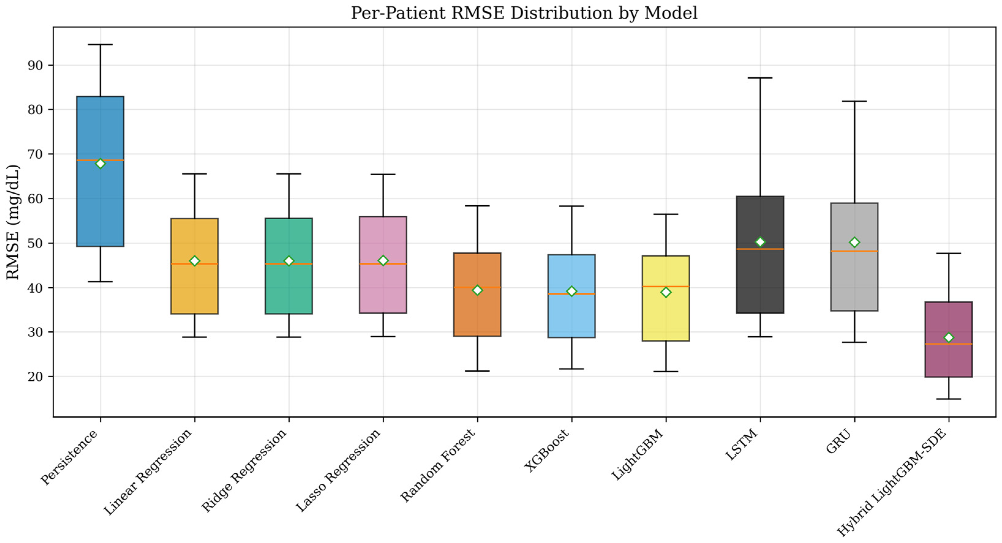
To determine whether observed performance differences are statistically meaningful, pairwise Wilcoxon signed-rank tests were applied to the per-patient RMSE vectors at a significance level of α = 0.05. Finally, SHAP TreeExplainer (version 0.46.0, https://shap.readthedocs.io) [22] was used to decompose the Hybrid LightGBM-SDE model predictions into additive feature contributions, providing a transparent view of which input variables—including the GIM-derived simulation statistics—drive the model’s decisions.

No data augmentation or oversampling techniques (such as SMOTE) were applied in this study. Blood glucose prediction is formulated as a regression task, making classification-based oversampling methods inapplicable. The natural concentration of predictions in Clarke zone A for well-performing models is a property of accurate prediction rather than a sampling artefact and is consistent with published results in the glucose prediction literature [3,4].

4. Results

4.1. Experimental Setup

All experiments were carried out on a standard desktop workstation equipped with an Intel multi-core CPU; no GPU acceleration was used. The software stack comprised Python 3.14, scikit-learn 1.7.2, XGBoost 3.1.2, LightGBM 4.6.0, and PyTorch 2.9.1. A global random seed of 42 was fixed throughout to ensure full reproducibility. The overall pipeline, from data ingestion through model evaluation, is illustrated schematically in Figure 1.

4.2. Main Results

Table 3. RMSE (mg/dL, mean ± std across patients) for all methods and prediction horizons. Bold indicates best performance per horizon.

Method	15 min	30 min	60 min	120 min
Persistence	55.75 ± 13.4	67.81 ± 16.8	80.08 ± 21.3	87.06 ± 25.3
Linear Reg.	30.28 ± 7.6	45.96 ± 11.4	54.56 ± 14.9	56.55 ± 15.7
Ridge Reg.	30.28 ± 7.6	45.97 ± 11.4	54.57 ± 14.9	56.55 ± 15.7
Lasso Reg.	30.41 ± 7.6	46.07 ± 11.4	54.64 ± 14.7	56.57 ± 15.7
Random Forest	26.88 ± 7.6	39.37 ± 10.7	46.56 ± 13.4	50.90 ± 15.3
XGBoost	26.02 ± 7.5	39.11 ± 10.6	46.30 ± 13.1	50.53 ± 15.0
LightGBM	25.97 ± 7.5	38.92 ± 10.5	46.43 ± 13.4	50.30 ± 15.3
LSTM	46.64 ± 16.2	50.21 ± 16.5	52.53 ± 17.2	53.85 ± 18.1
GRU	45.12 ± 14.1	50.11 ± 15.6	51.07 ± 16.9	53.02 ± 17.2
Hybrid LightGBM-SDE	22.42 ± 6.8	28.74 ± 9.4	33.89 ± 10.6	37.22 ± 11.7

and

Table 4. MAE (mg/dL, mean ± std across patients) for all methods and prediction horizons. Bold indicates best performance per horizon.

Method	15 min	30 min	60 min	120 min
Persistence	37.24 ± 10.0	46.15 ± 12.7	57.23 ± 16.8	64.04 ± 21.4
Linear Reg.	21.88 ± 5.7	31.76 ± 7.5	39.81 ± 10.1	42.13 ± 11.3
Ridge Reg.	21.88 ± 5.7	31.75 ± 7.5	39.81 ± 10.1	42.13 ± 11.3
Lasso Reg.	21.94 ± 5.6	31.74 ± 7.4	39.86 ± 10.0	42.11 ± 11.2
Random Forest	19.49 ± 5.9	27.61 ± 8.1	33.59 ± 10.7	37.37 ± 12.0
XGBoost	19.35 ± 5.9	27.74 ± 8.1	33.55 ± 10.4	37.17 ± 11.9
LightGBM	19.26 ± 5.9	27.48 ± 8.0	33.53 ± 10.5	36.94 ± 12.0
LSTM	32.06 ± 11.4	35.37 ± 12.1	37.86 ± 12.9	38.76 ± 13.9
GRU	31.01 ± 10.4	35.25 ± 11.4	36.91 ± 12.8	38.51 ± 13.4
Hybrid LightGBM-SDE	17.42 ± 5.5	22.16 ± 7.6	26.10 ± 8.9	28.48 ± 10.0

report, respectively, the RMSE and MAE achieved by each method at every prediction horizon, expressed as the mean ± standard deviation across the 34 patients. The Hybrid LightGBM-SDE model achieves the lowest error at every horizon. Among the remaining methods, the three gradient-boosted ensembles (LightGBM, XGBoost, and Random Forest) form a clearly separated second tier, followed by the linear regressors, while the recurrent neural networks and the persistence baseline trail behind.

Figure 2 provides a graphical view of how the RMSE evolves with an increasing prediction horizon for each method. The curves fan out as the horizon lengthens, reflecting the growing difficulty of prediction, but the Hybrid LightGBM-SDE model curve remains well below all others throughout.

4.3. Clarke Error Grid Analysis

From a clinical standpoint, the absolute magnitude of prediction error matters less than whether the error is likely to lead to a harmful treatment decision. The Clarke Error Grid addresses this question by classifying each predicted–actual glucose pair into one of five zones. Zone A predictions are clinically accurate, zone B predictions would lead to benign treatment decisions, and zones C through E represent errors of increasing clinical severity.

Table 5. Clarke Error Grid zone distribution (%) at the 30 min prediction horizon. Zones A + B are clinically acceptable; zones C–E represent clinically significant errors.

Method	Zone A	Zone B	Zone C	Zone D	Zone E
Persistence	51.76	41.62	1.45	5.08	0.09
Linear Reg.	63.63	34.03	0.06	2.22	0.05
Ridge Reg.	63.69	33.98	0.08	2.21	0.05
Lasso Reg.	63.68	33.96	0.07	2.23	0.05
Random Forest	70.32	28.31	0.36	0.93	0.07
XGBoost	69.60	29.06	0.33	0.97	0.04
LightGBM	70.19	28.35	0.37	1.03	0.07
LSTM	61.41	36.76	0.46	1.30	0.06
GRU	60.95	36.95	0.65	1.42	0.02
Hybrid LightGBM-SDE	77.73	21.98	0.01	0.26	0.02

reports the zone distributions at the 30 min horizon.

The Hybrid LightGBM-SDE model places 77.73% of its predictions in zone A and a further 21.98% in zone B, for a combined A + B rate of 99.71%. Only 0.26% of predictions fall in zone D, which corresponds to a failure to detect clinically significant hypo- or hyperglycaemia. The scatter plot in Figure 3 illustrates this concentration of predictions around the diagonal.

4.4. Per-Patient Variability

An important consideration for any glucose prediction method is whether it performs consistently across patients with different glycaemic profiles, or whether a favourable average masks poor accuracy for certain individuals. Figure 4 addresses this question with box plots of per-patient RMSE at the 30 min horizon. The Hybrid LightGBM-SDE model not only achieves the lowest median error but also exhibits the most compact interquartile range, suggesting that the benefit of the GIM-derived features extends to patients with widely differing levels of glycaemic variability.

4.5. Statistical Significance

Table 6. Selected pairwise Wilcoxon signed-rank test p-values at the 30 min horizon. Values below 0.05 indicate statistically significant differences.

	Hybrid	LightGBM	XGBoost	RF
LightGBM	<10−10	—	0.158	0.037
XGBoost	<10−10	0.158	—	0.270
Random Forest	<10−10	0.037	0.270	—
Linear Reg.	<10−10	<10−10	<10−10	<10−10
LSTM	<10−10	<10−10	<10−10	<10−10
Persistence	<10−10	<10−10	<10−10	<10−10

reports selected pairwise Wilcoxon signed-rank test p-values at the 30 min horizon. The Hybrid LightGBM-SDE model differs significantly from every other method (p < 10⁻¹⁰ in all cases). Among the three gradient-boosted ensembles, three pairwise comparisons were performed. The raw p-values are: LightGBM vs. Random Forest p = 0.037, LightGBM vs. XGBoost p = 0.158, and XGBoost vs. Random Forest p = 0.270. After applying the Holm–Bonferroni correction for multiple comparisons (3 tests), the adjusted p-value for the LightGBM vs. Random Forest comparison becomes p_adj = 0.112, which does not reach significance at α = 0.05. Thus, none of the three ensemble methods differ significantly from one another after correction, confirming that they form a homogeneous performance group. A similar pattern holds for the two recurrent networks, whose mutual comparison gives p = 0.66.

4.6. Ablation Study: GIM Feature Contribution

To isolate the contribution of the stochastic simulation features, an ablation experiment compared standard LightGBM (37 base features) against the full Hybrid LightGBM-SDE model (37 base plus 8 GIM features). The results, presented in

Table 7. Ablation study: effect of GIM-derived features on LightGBM performance. RMSE is expressed in mg/dL.

Horizon	LightGBM	Hybrid (+GIM)	Improvement (%)
15 min	25.97	22.42	13.6
30 min	38.92	28.74	26.2
60 min	46.43	33.89	27.0
120 min	50.30	37.22	26.0

, show a consistent improvement at every horizon. At 15 min, the gain is a modest but meaningful 13.6%, rising to 26.2% at 30 min and plateauing near 27% at 60 min. This pattern makes intuitive sense: at very short horizons, the most recent glucose readings are already highly predictive, leaving little room for the simulation to add value, whereas at longer horizons, the forward-looking trajectory information encoded in the GIM statistics becomes increasingly difficult to infer from backward-looking lag features alone.

4.7. Feature Importance Analysis

SHAP TreeExplainer was applied to the trained Hybrid LightGBM-SDE model at the 30 min horizon, and the resulting feature importance ranking is shown in Figure 5. The most influential predictors are, as expected, the most recent glucose lags (bg_lag_1 and bg_lag_2), which carry direct information about the current metabolic state. Notably, however, three GIM-derived features—gim_mean, gim_p50 (the median of the simulated distribution), and gim_std—rank among the top ten, confirming that the stochastic simulation supplies complementary predictive signal that is not redundant with the empirical lag and rolling-statistics features. Insulin-on-board also appears prominently, reflecting the well-known clinical importance of residual active insulin in shaping short-term glucose trajectories.

4.8. Prediction Validation Cases

To get a qualitative sense of model behaviour, Figure 6 and Figure 7 overlay the Hybrid LightGBM-SDE model’s predictions on the actual glucose traces for two representative patients from the synthetic D1NAMO-equivalent dataset at the 30 min horizon. In both cases, the model tracks the overall trajectory well, including meal-related excursions and overnight drifts. Predictably, the largest deviations occur during rapid glucose transitions—steep postprandial rises or sharp insulin-induced drops—where even a small timing error translates into a large amplitude mismatch.

4.9. Computational Cost

Table 8. Computational cost at the 30 min horizon. Training on ~40,900 samples, inference on ~10,200 samples. Times include hyperparameter selection where applicable.

Method	Training (s)	Inference (s)
Persistence	<0.01	<0.01
Linear Regression	0.07	<0.01
Ridge Regression	29.0	<0.01
Lasso Regression	23.4	<0.01
Random Forest	163.6	0.09
XGBoost	2.9	<0.01
LightGBM	2.7	<0.01
LSTM	95.8	<0.01
GRU	120.6	<0.01
Hybrid LightGBM-SDE	2.3	<0.01

reports training and inference times at the 30 min horizon. The Hybrid LightGBM-SDE model trains in 2.3 s—comparable to standalone LightGBM (2.7 s) and orders of magnitude faster than both Random Forest (163.6 s, dominated by the cost of growing 200 deep trees) and recurrent networks (96–121 s of CPU-bound back-propagation). The training times reported in Table 8 do not include GIM feature pre-computation, which is performed once during the preprocessing phase. GIM pre-computation requires approximately 3–15 s per patient per horizon (scaling linearly with horizon length), totalling roughly 4.4 min for the D1NAMO-equivalent dataset (9 patients) and 12.2 min for the HUPA-UCM-equivalent dataset (25 patients) across all four horizons. For the full benchmark, the total GIM overhead is approximately 17 min. This cost is incurred only once and is amortised across all training runs. Inference is near-instantaneous for all methods (<0.01 s in every case except Random Forest), making any of them viable for real-time deployment on modern hardware.

5. Discussion

5.1. Key Findings

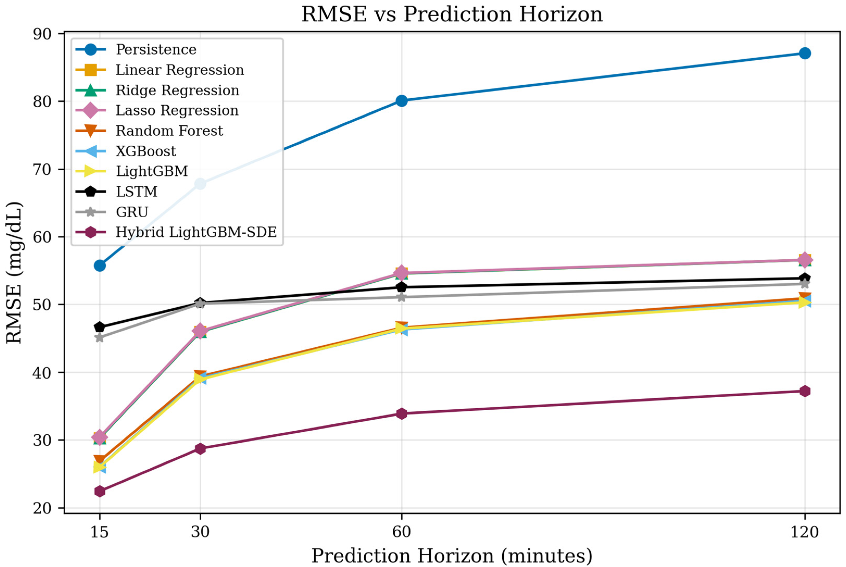
Perhaps the most striking outcome of this benchmark is the clear superiority of gradient-boosted ensemble methods over both classical linear models and recurrent neural networks. LightGBM, XGBoost, and Random Forest consistently outperform linear and ridge regression across every horizon, with the gap widening at longer look-ahead times. At the 120 min horizon, for example, LightGBM records an RMSE of 50.30 mg/dL against 56.55 mg/dL for linear regression—an 11% reduction that reflects the ability of tree ensembles to capture the non-linear interactions between insulin action, carbohydrate absorption, and circadian effects that linear models cannot represent.

The relatively poor performance of the LSTM and GRU networks was, at first glance, unexpected, given the sequential nature of CGM data and the success that recurrent architectures have enjoyed in natural-language and speech tasks. At the 15 min horizon, both RNN variants produce RMSE values near 46 mg/dL—almost double the 26 mg/dL value achieved by LightGBM. Several factors likely contribute to this result. The total sample size (34 patients) is modest by deep learning standards, limiting the capacity of the networks to generalise. The carefully engineered lag and rolling-statistics features already encode the temporal structure that the recurrent units would otherwise need to learn from raw sequences. And the restriction to CPU-only training constrained the number of epochs and the breadth of architecture search that could feasibly be explored.

The ablation experiment isolating the contribution of the GIM-derived features reveals that these eight simulation-based statistics reduce the RMSE by 13.6% at 15 min and by as much as 27% at 60 min. The mechanism behind this improvement is intuitive: at short horizons, the most recent glucose readings are inherently informative, so the marginal value of a physiological simulation is limited. As the prediction window stretches, however, the lagged features become increasingly stale, and the forward-looking trajectory information encoded in the SDE simulation fills a gap that no backward-looking statistic can bridge.

From a clinical safety perspective, the Hybrid LightGBM-SDE achieves a combined Clarke Error Grid A + B rate of 99.71% at the 30 min horizon. Critically, only 0.26% of predictions fall in zone D, which corresponds to a failure to flag a clinically significant glucose excursion. These figures suggest that the model’s errors, while non-zero, are overwhelmingly benign and unlikely to provoke harmful treatment decisions.

5.2. Comparison with the Literature

The RMSE values reported here are broadly in line with those found in the wider literature. Published studies typically report values of 15–30 mg/dL at the 15–30 min horizon and values of 30–50 mg/dL at the 60–120 min horizon [3,4]; the Hybrid LightGBM-SDE model sits comfortably within or below these ranges. The observation that gradient boosting outperforms deep recurrent networks on structured, tabular-style feature matrices is consistent with the findings of Grinsztajn et al. [23], who showed that tree-based models remain highly competitive with neural networks on typical tabular data, often matching or surpassing them when features are well engineered. For clinical deployment, gradient boosting carries the additional advantages of fast training, low memory footprint, and native support for interpretability tools like SHAP.

Recent work on Transformer architectures for tabular data—including TabNet [24], FT-Transformer [25], and TabTransformer [26]—has produced mixed results relative to gradient boosting. Grinsztajn et al. [23] demonstrated that tree-based methods consistently match or outperform deep learning on typical tabular datasets, a finding corroborated by our results. In the specific domain of glucose prediction, attention-based architectures have been explored [12,17], but their advantage tends to materialise only with large training sets and GPU resources—conditions not met in the present benchmark (34 patients, CPU-only). Including Transformer baselines—particularly temporal fusion Transformers designed for multi-horizon forecasting—is an important direction for future work, especially as larger open-access CGM datasets become available.

The computational cost analysis (Table 8) reveals a striking efficiency gap between ensemble methods and deep learning. XGBoost trains in 2.9 s and LightGBM in 2.7 s, compared to 95.8 s (LSTM) and 120.6 s (GRU)—approximately 35–45× faster. Critically, the faster ensemble methods also achieve substantially better RMSE: LightGBM achieves a value of 25.97 mg/dL at 15 min versus LSTM (46.64 mg/dL) and GRU (45.12 mg/dL). This combined accuracy-per-compute advantage makes tree-based ensembles strongly preferable for resource-constrained clinical environments, including edge devices integrated with CGM sensors, where both training speed (for periodic model updates with new patient data) and inference latency (for real-time glucose alerts) are critical constraints. The Hybrid LightGBM-SDE maintains this efficiency (2.3 s training) while achieving the best overall accuracy, though GIM feature pre-computation adds a one-time overhead of approximately 3–12 min per dataset depending on cohort size.

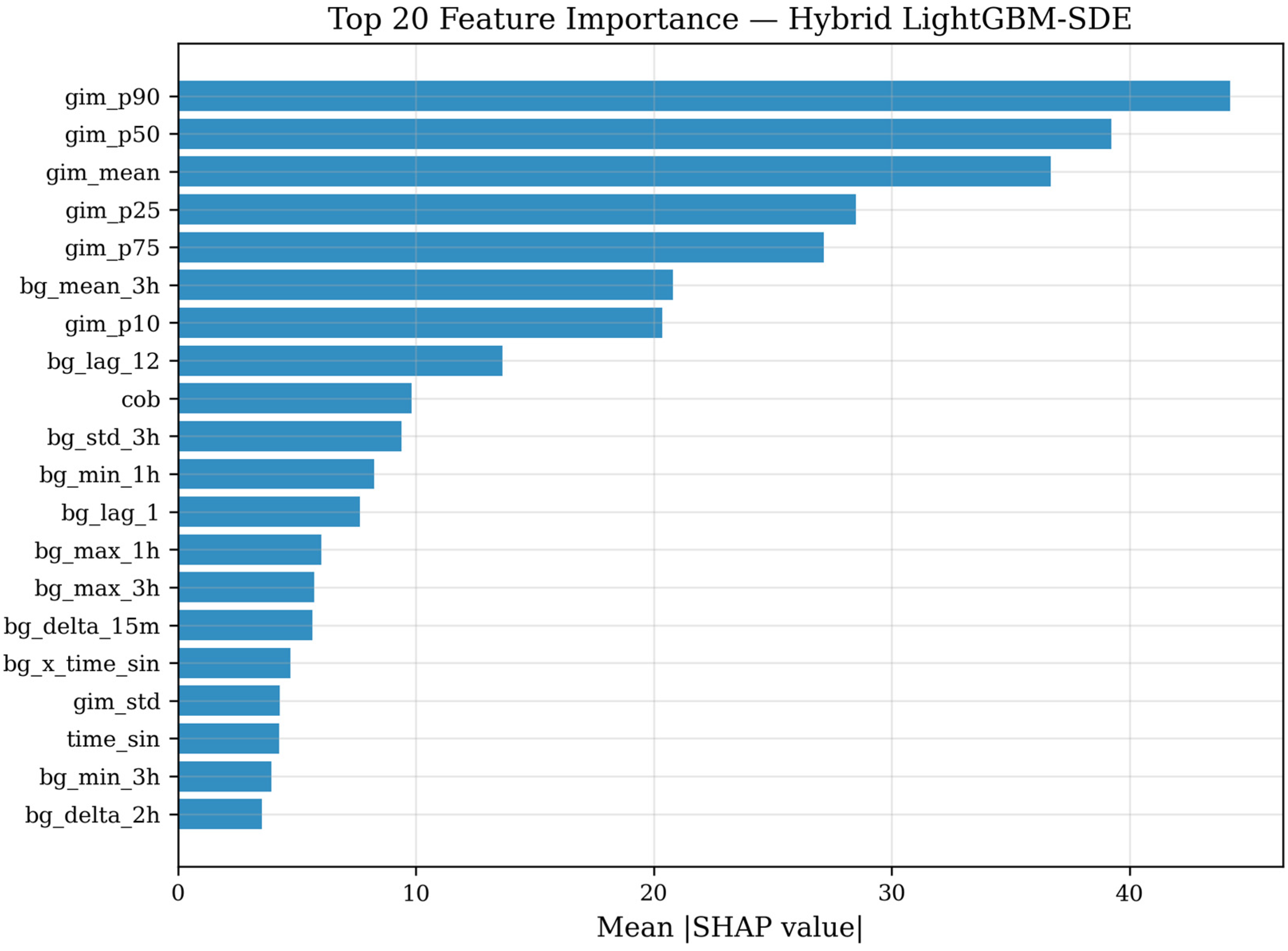
From the perspective of clinical trust and adoption, the interpretability of ensemble methods is a significant advantage. Tree-based models natively support feature importance via split gain and split frequency metrics, but more importantly, SHAP TreeExplainer [22] provides theoretically grounded, per-prediction feature attributions in polynomial time. As shown in Figure 5, the SHAP analysis reveals that the Hybrid LightGBM-SDE’s predictions are driven by a clinically intuitive combination of recent glucose values (bg_lag_1 and bg_lag_12), forward-looking GIM statistics (gim_p90, gim_p50, and gim_mean), rolling means (bg_mean_3h), and metabolic state indicators (carbs-on-board and insulin-on-board). This transparency enables clinicians to understand why the model predicts a future glucose drop—for instance, because insulin-on-board is high while the GIM forward simulation projects a declining trajectory. In contrast, LSTM and GRU networks operate as black boxes with no native mechanism for per-prediction explanations, which remains a significant barrier to their clinical adoption despite advances in post hoc RNN interpretability methods.

5.3. Limitations

Several limitations of this study should be borne in mind when interpreting the results. First, and most importantly, the benchmark was conducted on physics-based synthetic data rather than on the original clinical recordings. Although the synthetic generator incorporates realistic physiological dynamics, circadian variation, sensor noise, and data gaps, it cannot fully replicate the complexity and heterogeneity of real CGM time series. We plan to repeat the full experiment on the real D1NAMO and HUPA-UCM datasets once download access to the respective repositories is restored.

Second, the tree-based ensembles were trained with fixed, commonly used hyperparameters rather than with exhaustive grid or Bayesian search. While this choice was made to keep computation tractable and to reflect a realistic “out-of-the-box” usage scenario, it means that the reported performance of Random Forest, XGBoost, and LightGBM may not represent their theoretical ceiling. Third, the LSTM and GRU networks were explored with a single architecture and a limited training budget on CPU; GPU-accelerated training with broader architecture search might narrow or close the gap with the ensemble methods.

Fourth, the GIM parameters used in the stochastic simulation are population-level averages drawn from the original Bergman study. Estimating patient-specific parameters—for instance, by fitting the SDE system to each individual’s historical glucose and insulin data—could further sharpen the hybrid model’s predictions. Finally, each patient’s data were split only once (80/20 chronological); repeated splits or nested cross-validation would yield tighter confidence estimates around the reported metrics.

5.4. Practical Implications

From a deployment standpoint, the Hybrid LightGBM-SDE model presents a compelling profile. It trains in roughly two seconds on a standard CPU, making it feasible to retrain or fine-tune the model as new patient data accumulate. Inference is effectively instantaneous, well within the latency budget of a real-time CGM application running on a smartphone or insulin pump controller. The SHAP decomposition offers clinicians a transparent explanation of each prediction, which can support trust-building and regulatory review. And the GIM simulation component anchors the model in established physiology, offering a layer of interpretability that purely data-driven black-box approaches lack.

6. Conclusions

This paper has presented a systematic benchmark of ten machine learning methods for blood glucose prediction in type 1 diabetes, evaluated across two datasets encompassing 34 patients, four prediction horizons spanning 15 to 120 min, and a battery of error, clinical safety, and statistical significance metrics. The proposed Hybrid LightGBM-SDE model—which enriches a gradient-boosted decision tree with features drawn from Monte Carlo simulations of a stochastic glucose–insulin model—achieves the lowest error at every horizon, with RMSE values of 22.42, 28.74, 33.89, and 37.22 mg/dL at 15, 30, 60, and 120 min, respectively.

The experimental evidence supports several broader conclusions. Gradient-boosted ensembles consistently outperform both linear regressors and recurrent neural networks when applied to well-engineered tabular features derived from CGM data. Stochastic physiological simulation features provide meaningful and statistically significant improvements—ranging from 13.6% to 27.0%—with the largest gains appearing at longer horizons where backward-looking empirical features lose their predictive power. The hybrid model’s predictions are overwhelmingly clinically safe, with 99.71% of 30 min forecasts falling within the acceptable zones of the Clarke Error Grid. Training and inference are fast enough for real-time clinical use.

6.1. Clinical Decision Support Pathway

The benchmark results suggest a practical model selection strategy for different clinical scenarios. For short-horizon glucose alerts (15 min predictions, e.g., hypoglycaemia warnings), any of the three ensemble methods (LightGBM, XGBoost, and Random Forest) provides acceptable accuracy with fast training. For insulin dosing support (30–60 min predictions), the Hybrid LightGBM-SDE model is recommended due to its advantage of a 26–27% RMSE and its 99.71% clinical safety rate. For meal planning and longer-term trend forecasting (120 min horizon), the hybrid model’s advantage is most pronounced (26% improvement over standalone LightGBM), making it the clear choice.

A deployment pathway from benchmark to bedside would proceed as follows: (1) retrospective validation on real CGM datasets to confirm performance outside synthetic data; (2) prospective clinical study comparing model-assisted decisions with standard care; and (3) regulatory submission under the FDA’s guidance on AI/ML-based Software as a Medical Device (SaMD) [27]. The modular benchmark pipeline provided with this paper is designed to facilitate step (1) by accepting new datasets with minimal configuration. While addressing different engineering challenges, earlier contributions by Mitev [28,29,30] demonstrate how well-defined system architectures can support reliable and reproducible outcomes.

The benchmark establishes a foundation for developing autonomous glucose control systems (artificial pancreas). In such systems, optimising solely for RMSE is insufficient—clinical safety (minimising zone C–E predictions) must be jointly optimised. Future work should explore composite metrics that combine statistical accuracy with clinical safety through Pareto-optimal model selection. The Hybrid LightGBM-SDE model already achieves a favourable position on both axes (lowest RMSE and highest Zone A + B percentage), suggesting that it is a strong candidate for closed-loop control applications.

6.2. Future Directions

Validating the benchmark on the original D1NAMO and HUPA-UCM clinical recordings remains the most immediate priority. Beyond that, transfer learning offers a promising pathway to personalisation: a general model pre-trained on multi-patient data could be fine-tuned on a new patient’s limited CGM history (e.g., 3–7 days), enabling rapid adaptation without extensive per-patient training data. For tree-based models, incremental boosting allows efficient model updating; for deep learning models, standard fine-tuning of pre-trained RNN weights could enable few-shot adaptation to individual glucose dynamics.

Further directions include personalising the GIM parameters for individual patients, incorporating additional data streams such as physical activity and stress biomarkers, and conducting prospective trials within a closed-loop insulin delivery system. The full source code, evaluation scripts, and synthetic data generators accompanying this paper are publicly available to support reproducibility and to serve as a shared baseline for future work.