Evaluating Handcrafted Image Descriptors for Defect Detection in the X-Ray Inspection of Turbine Blade Castings: A Feature Separability Study

Abstract

The industrial X-ray inspection of turbine blade castings requires reliable and auditable decision support, yet defect indications are subtle, and data availability is limited. This study quantitatively assesses the diagnostic potential of handcrafted image descriptors by evaluating class separability in feature space, independently of any trained classifier. The dataset comprises 1600 16-bit DICOM radiograms of 200 blades (eight views per blade), including 156 defective images with 207 localized defects. Standardized 32 × 32 ROI patches were sampled randomly in the vicinity of indications and from defect-free regions to reduce sample correlation and to emulate localization uncertainty. Feature vectors were extracted using five descriptor families—first-order statistics, GLCM/Haralick, FFT and wavelet (DWT) features, Gabor filters, and LBP—and the standardized z-score. Separability was ranked using complementary distribution-based and distance-based metrics grouped into three sets, and the results were min–max-normalized to enable TOP-5 comparisons. Spectral descriptors, particularly DWT wavelets and FFT combined with DWT, consistently achieved the highest scores in distributional metrics, supporting a lightweight screening profile. In contrast, richer combinations dominated multidimensional geometric metrics, indicating benefits from multi-perspective representations for offline analysis. The proposed metric-driven framework provides an interpretable basis for representation selection prior to classifier development under industrial constraints.

1. Introduction

Quality control is one of the key stages of the production cycle. For critical components, such as the hot-section gas turbine blades of an aircraft engine, its outcome directly translates into operational safety and maintenance costs [1]. In industrial practice, inspection is often a “bottleneck”; therefore, the demand is increasing for tools that automate the analysis of inspection images and for solutions that support operators in decision-making [2]. Robotic solutions constitute an increasingly large part of manufacturing processes [3,4], including the operation of quality control workstations employing non-destructive testing methods [5,6,7,8]. Such an approach allows human resources to be shifted towards the interpretation and resolution of ambiguous cases, which is particularly important in X-ray radiography: the time-consuming and monotonous nature of visual NDT evaluation affects the psychophysical condition of employees and, consequently, the quality of the inspection process [9]. From an automation perspective, the nature of the data remains a challenge: X-ray images are information-rich yet difficult to interpret, and defects may be only a few pixels in size, while their visibility depends on contrast settings. Under such conditions, both humans and learning-based algorithms may be sensitive to acquisition variability and different types of disturbances [10].

Turbine blades produced with investment casting methods may exhibit a range of manufacturing discontinuities, most commonly including porosity, shrinkage-related defects and inclusions, as well as process-related defects such as cold shuts and cracks or hot tears [11,12]. It is worth noticing that X-ray radiography is primarily suited for detecting internal volumetric defects that introduce measurable density or thickness variations—particularly pore voids, shrinkage cavities, porosity, and material inclusions—whereas planar discontinuities (e.g., cracks) may be challenging to detect unless oriented favorably to the radiation beam. Hence, surface-breaking imperfections are typically addressed using complementary surface methods (e.g., fluorescent penetrant inspection) [13].

In response to the complexity of images and the demand for automation, learning-based methods have become a natural direction in recent years, including deep learning models that can build representations without manual feature engineering. In radiographic quality control, these methods have most often been implemented in three types of applications: classification [14,15], object detection [16,17], and segmentation [18]. However, their effectiveness is frequently strongly dependent on large, balanced, and consistently labeled datasets. Their availability in the aerospace industry is limited due to confidentiality constraints and the low number of defective parts. In such cases, engineering practice often relies on fine-tuning models on domain-specific data, yet public X-ray datasets of casting defects remain scarce and small [19]. Data augmentation is also applied [20], which partially alleviates data scarcity but does not fully address robustness to acquisition variability and the interpretability of decisions. Consequently, when access to large and consistently labeled datasets is limited, and traceability and auditability are required, an approach based on an interpretable image representation and a quantitative assessment of its class-separating capability is justified. Therefore, manually designed descriptors remain particularly useful, as they are computationally “lightweight” and interpretable and can operate with fewer examples [21]. The literature reports numerous examples of image classification using classical classifiers: a wavelet transform combined with k-NN was applied in [22], whereas [23] compared SVM, random forests, and the naive Bayes classifier. In [24], the Fourier transform was included in the feature extraction stage, and the use of a fractal transform for image recognition was presented in [25].

In critical applications, such as aviation, predictive performance alone is not sufficient. The transparency of the decision-making process is also required, as well as decision traceability, auditability, uncertainty assessment, and unambiguous rules for handling borderline cases. For these reasons, explainable artificial intelligence (XAI) methods, hybrid approaches, and human-in-the-loop solutions are being developed to increase trust in the system and the safety of the inspection process [26,27]. In [28], a systematic literature review of quality assurance and quality management was conducted, with a particular focus on AI and XAI methods. It was shown that XAI implementation in industrial practice remains limited, due to the lack of standardized metrics for explanation assessment and reference datasets enabling an objective comparison of results. An approach is justified in which emphasis is placed on the feature layer and on a comparable assessment of its properties before selecting a specific decision model—especially since, under industrial conditions, repeatability, stability with respect to acquisition variability, and the possibility of validation for subsequent production batches are crucial. In practice, this means that feature families ensuring consistent class separation under different conditions should be identified first, and only then should the classification mechanism be selected for an already verified representation. This approach is also supported by the practical deployment context. During cooperation with a precision foundry, the need to automate the analysis of X-ray images of blade castings was identified, where inspection constitutes a process bottleneck. Therefore, the present work focuses on a quantitative assessment of the ability of different feature families to separate the classes “good” and “defect”. This constitutes a first stage in building a stable solution that supports inspectors, reduces assessment time, and limits costs while maintaining requirements typical for critical applications.

The remainder of this paper is organized as follows: Section 2 describes the dataset and methods used in this research. It consists of three parts. Section 2.1 describes the dataset and the sample preparation procedure based on image patches. Section 2.2 presents feature families and their extraction methods. In this work, families of manually designed descriptors were compared within a unified analysis framework based on 32 × 32 image patches. Section 2.3 defines separability metrics and the evaluation procedure. Class separability was evaluated using sets of distributional and distance-based metrics to verify the stability of conclusions. Section 3 discusses the results together with deployment recommendations. Finally, Section 4 provides a discussion of the obtained results, and Section 5 presents the final conclusions.

2. Materials and Methods

2.1. Research Materials

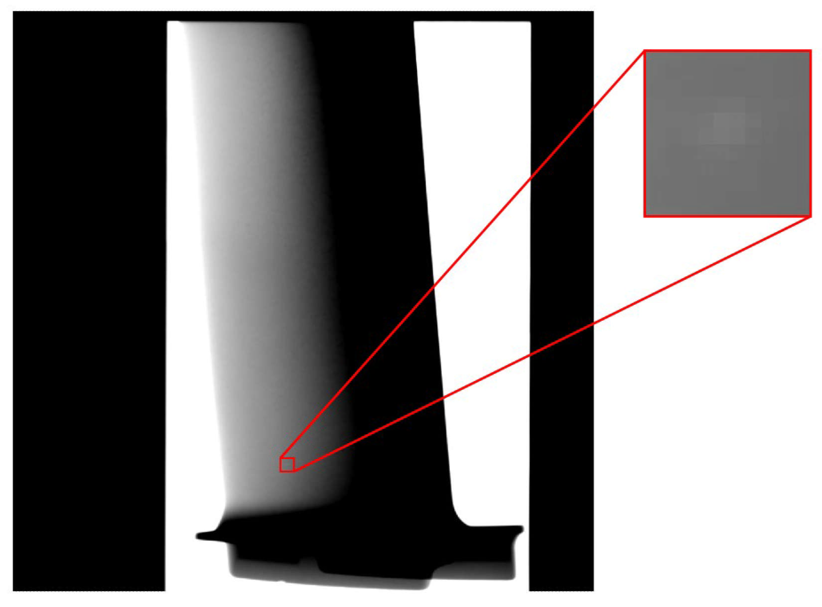
The dataset used in the presented study consists of X-ray images of aircraft engine blade castings stored as DICOM files. Each image has a resolution of 1024 × 1024 pixels and a 16-bit grayscale depth (Figure 1). In total, 1600 images depicting 200 blades are available (eight views per blade). Within the dataset, 156 images of blades with defects were identified; some of them contain multiple defect occurrences, resulting in a total of 207 localized defects.

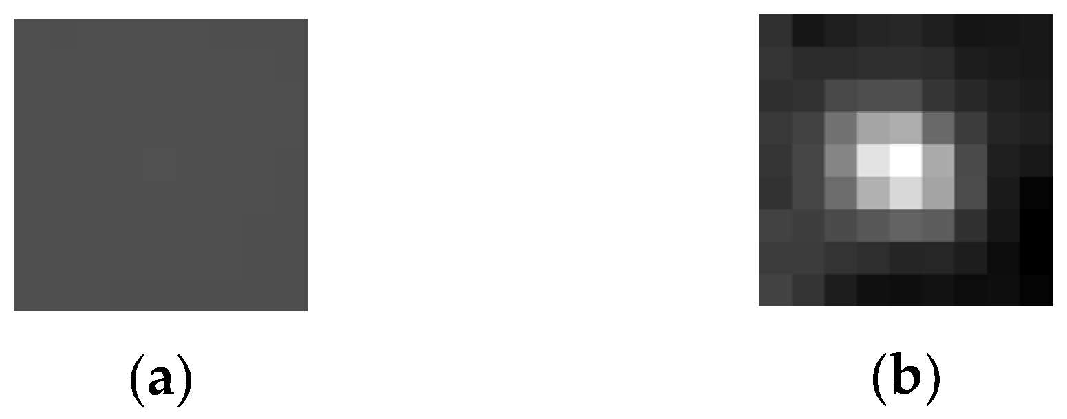
The diameter of the considered defects is in the range of 4–8 pixels, which means that the defect area relative to the full image area is on the order of 10⁻⁵–10⁻⁴ (Figure 2). Such a small defect size, combined with the high grayscale resolution (16 bits), justifies an analysis based on descriptors sensitive to subtle texture changes and local inhomogeneities.

A key aspect of data preparation is preserving information on the dynamic range and grayscale resolution. DICOM X-ray images are typically encoded with 16-bit precision, and conversion to 8-bit representation at the initial exploration stage may lead to the loss of subtle contrast differences between pixels. Therefore, the analysis was performed at the native bit depth, and all normalization operations were implemented in a reproducible and reversible manner.

2.2. Feature Extraction

The aim of this work is to assess feature quality in the context of small defects; therefore, the analysis was conducted on standardized ROI patches with a fixed size of 32 × 32 pixels. The window size was selected based on the authors’ previous work, where the influence of patch dimensions on class discrimination was evaluated [29]. In this paper, for each localized defect, several windows were generated by controlled shifts with respect to the center point (x, y). The window sizes that were evaluated were the following: 9 × 9, 16 × 16, 32 × 32, 64 × 64, 84 × 84, and 1024 × 1024. The results presented in this paper indicate that the window size that yields the best results for this particular task is 32 × 32 pixels. It increased robustness to small localization errors and introduced realistic sample variability. The chosen window size was a compromise between capturing local intensity and texture variations and limiting the “blurring” of information related to the indication–defect. Moreover, this enables fast computations and reduces the dimensionality of the feature vector in the comparative study. Based on these results, a dataset of 32 × 32 patches was used in this study.

The 32 × 32 patches were generated randomly to increase sample diversity and reduce correlation between neighboring fragments. For the “no defect” class, windows were sampled from the part region, whereas for the “defect” class, windows were sampled in the vicinity of the indication (locally around the defect location) such that the defect was included within the patch. In contrast to exhaustive sliding window scanning with a 1-pixel stride, random sampling promotes more diverse examples for the same number of samples (Figure 3). This sampling strategy imitates localization uncertainty, stabilizes the feature description against small acquisition changes, and facilitates the comparison of feature families under conditions close to industrial practice. The number of samples was selected to obtain a 1:1 class balance. It is worth noting that component-level splitting is the appropriate strategy for downstream model evaluation and unbiased generalization assessment. Therefore, the subsequent stages of the proposed pipeline explicitly apply grouping by part to avoid bias introduced by sample correlation.

It is worth emphasizing that the dataset used in this study was provided by an industrial partner as part of an ongoing collaboration. As a consequence, the authors had no possibility to intervene in or experimentally control the acquisition process of X-ray images (e.g., exposure parameters, detector settings, hardware configuration, or reconstruction settings). Therefore, the presented evaluation focuses solely on feature selection and class separability under the acquisition conditions available in the industrial workflow. A systematic robustness study across varying acquisition settings is beyond the scope of the present work and is identified as future work when multi-setting data or acquisition metadata become available.

Since no classifier was trained and the analysis was limited to class separability in the feature space, all metrics were computed on the complete set of samples (windows). To mitigate artifacts resulting from strong sample dependence, random window sampling was applied, and a part identifier was retained in the data structure (enabling an object-wise data split in future work, if the analysis is extended to model training). Feature extraction transforms an image or an ROI patch into a feature vector that compactly describes the selected properties of intensity, structure, and texture. To ensure comparability, all features were computed using a consistent procedure, and method parameters were kept fixed throughout the experiment. The features considered in the analysis include brightness histogram statistics, textural features, spectral features (FFT and wavelet-based), Gabor filters, and local binary patterns (LBPs).

Because casting defects in X-ray images may exhibit arbitrary orientation, directional averaging was applied in several cases, or feature vectors were constructed by aggregating responses over multiple orientations. This increases rotation robustness at the cost of higher dimensionality. Both variants were included in the comparison: directional descriptors and direction-averaged descriptors. All experiments were conducted in MATLAB R2024b using the Image Processing Toolbox, Wavelet Toolbox, and Statistics and Machine Learning Toolbox.

Feature vectors were derived from grayscale X-ray images after an initial pre-processing stage (detector corrections, background equalization, and contrast standardization). Six descriptor families were considered as the basis for the comparative analysis: first-order statistical features, GLCM/Haralick textural features, FFT spectral features, multiscale features based on the DWT wavelet transform, Gabor filter-based features, and local LBP features.

Feature extraction was performed independently for each family (

Table 1. Feature families and key parameters.

Feature Family	Abbreviation	Parameters	Results
Statistical	STAT	First-order statistics computed from the pixel intensity distribution (global histogram).	Mean intensity, standard deviation, skewness, kurtosis, entropy.
Textural	GLCM	Gray-level co-occurrence matrix computed for four offsets (directions) $\left[0,1],\left[-1,1\right],\left[-1,0\right],[-1,-1\right]$; Symmetric = true; gray-level quantization with NumLevels = 8; features aggregated by averaging across directions.	Fourteen Haralick texture features (computed per direction and averaged), yielding a 14-dimensional GLCM feature vector per sample.
Fast Fourier Transform	FFT	2D FFT (2D-DFT) applied to the image; analysis performed on the magnitude spectrum $\mid F(u,v)\mid$.	Global spectral descriptors derived from $\mid F(u,v)\mid$, such as mean magnitude, standard deviation of magnitude, and spectral energy.
Digital Wavelet Transform	DWT	Two-level 2D discrete wavelet decomposition using Daubechies wavelet db4; subbands $LL,LH,HL,HH$ at each level.	Statistical and energy descriptors of wavelet coefficients, computed either globally from the concatenated coefficient vector or separately per subband (e.g., mean, variance/standard deviation, and energy of coefficients).
Gabor Filters	GABOR	Gabor filter bank with wavelengths $\lambda \in \left\{4,8,16\right\}$ and orientations $\theta \in \{0^{°},{45}^{°},{90}^{°},{135}^{°}\}$; filter responses obtained using magnitude output.	Statistical descriptors of filter responses per wavelength–orientation pair (e.g., mean, standard deviation, and energy of the response magnitude), concatenated into a single feature vector.
Local Binary Patterns	LBPs	Rotation-invariant uniform LBPs (RIU2) with radius R = 1 and P = 8 sampling points.	Normalized RIU2-LBP histogram (10-dimensional) used as the LBP feature vector per sample.

) on 32 × 32 patches; subsequently, in the combined analysis, the resulting descriptors were concatenated to form different feature set combinations. Within the statistical feature family (STAT), the arithmetic mean, standard deviation, skewness, kurtosis, and image entropy were computed. For textural features (GLCM), co-occurrence matrices were calculated in four directions (offsets: [0, 1], [−1, 1], [−1, 0], [−1, −1]) with enforced symmetry, and 14 Haralick measures were then derived; final values were aggregated as the mean across directions. Numerical artifacts were handled by replacing NaN/Inf values with zeros.

Spectral features comprised descriptors of the magnitude of the 2D FFT and the wavelet transform (DWT). For FFT, the statistics of the spectrum magnitude or spectral energy were used together with mean/maximum measures, whereas for DWT, a two-level decomposition (wavedec2, db4) was applied, and coefficient summaries were computed (mean, standard deviation/variance, and energy). Gabor features (GABOR) were implemented using a filter bank (is this an appropriate name) with wavelengths [4,8,16] and orientations from 0° to 135° in 45° steps; the feature vector was constructed from simple response statistics (mean, variance, skewness, kurtosis), information measures (entropy, energy), contrast, and spatial characteristics (mean local variance and the number of local maxima). Finally, local binary pattern (LBP) features were extracted using radius R = 1 and P = 8 neighbors.

2.3. Class Separability Metrics

The quality of individual feature extraction methods was assessed using a set of metrics describing class separability in the feature space. Both one-dimensional measures and multidimensional measures were applied, operating on mean vectors, covariance matrices, or directly on the distributions of feature values in the two classes. Two complementary metric groups were considered: distribution separability metrics (FDR [30], Bhattacharyya [31], JSD [32], Silhouette [33]) and distance-based metrics [34] (Mahalanobis, Euclidean, cosine, Wasserstein, Canberra).

All metrics were computed in MATLAB based on the feature matrix and class labels. For per-dimension measures (FDR, Bhattacharyya, JSD), a score was obtained for each feature and then averaged to yield a single value for a given extraction method. For multidimensional measures (Mahalanobis, Euclidean, cosine, Canberra), class mean vectors were used, whereas the Wasserstein metric was computed as an approximate transport cost between sorted values. The Silhouette measure was included as an auxiliary indicator of geometric compactness and separation of classes in the feature space (rather than a distribution measure sensu stricto), allowing for verification that high separability is not driven solely by a single divergence. It was computed in the standard manner based on within- and between-cluster distances in the feature space. For comparison purposes, all basic metric values were normalized using min–max scaling to the [0, 1] range within the set of analyzed methods; 1 denotes the best result for a given metric, and 0 denotes the worst.

For each tested feature combination, several separability metrics were computed and reported: both raw metric values and aggregated scores for ranking. Within each metric set (A, B, C), each metric was min–max-normalized to the [0, 1] range using the minimum and maximum values observed across all tested feature combinations in that set. The aggregated score was then computed as the (unweighted) mean of the normalized metrics within the set. Therefore, the aggregated scores should be interpreted as relative ranking indicators within the same table, not as absolute performance bounds and not for cross-set comparisons.

3. Results

Clear differences between feature families are already visible at the level of individual metrics. The FDR, Bhattacharyya, and JSD indicate very high separability for spectral features, particularly those based on the wavelet transform and its combinations with FFT. This suggests that defect-related information in X-ray images is strongly associated with changes in the multiscale structure of the image and its frequency components.

In contrast, the Silhouette measure often assigns high values to textural feature sets (textural/GLCM and their combinations), indicating the formation of compact clusters in the feature space. However, a high Silhouette score does not necessarily imply the largest difference in class means; therefore, it is treated as a complementary measure reflecting feature space structure rather than a single decisive selection criterion.

Within distance-based metrics, the highest scores are obtained by multi-family combinations (e.g., statistical + textural + FTT + wavelets + Gabor + LBP). This indicates that combining information on global brightness level (statistics), local texture (GLCM and LBP), directional structure (Gabor), and scale/frequency content (FFT and wavelets) increases the distance between class centroids and improves separability in a geometric sense. The trade-offs are a higher feature dimensionality and increased computational cost.

Overall, two practically useful strategies are indicated: simple, low-dimensional spectral feature sets (DWT, FFT + DWT), yielding excellent performance in distributional measures (FDR/Bhattacharyya/JSD), and richer feature combinations that perform consistently well in distance-based measures and may better capture defect variability, albeit at higher computational complexity.

Table 2. TOP-5 methods for Set A of metrics.

Method	FDR	Bhattacharyya	JSD	Silhouette	ScoreA
DWT	1.000	1.000	1.000	0.963	0.991
FFT + DWT	0.894	0.977	0.880	0.949	0.925
FFT	0.788	0.954	0.759	0.949	0.863
STAT + FFT + DWT	0.581	0.675	0.577	0.949	0.696
STAT + DWT	0.504	0.570	0.509	0.963	0.636

summarizes the five best methods (or method combinations) for Set A, where the ranking is determined by the mean of four separability metrics (FDR, Bhattacharyya, JSD, and Silhouette), with all values normalized to the 0–1 range. Set A favors solutions that provide a clear separation of feature distributions between the “good” and “defect” classes without requiring a complex decision model. The highest rank is achieved by wavelets alone (ScoreA ≈ 0.99), indicating that multiscale DWT coefficients capture image structure changes characteristic of casting defects. The second position, “FTT + DWT”, suggests complementarity: FFT provides global frequency–energy information, whereas DWT localizes disturbances in both scale and space. Subsequent TOP-5 entries typically involve multi-method combinations; however, under Set A, their gain is often moderate—additional feature families increase dimensionality but do not always yield proportional improvements in distribution-based metrics. In practice, the results in Table 2 support a “lightweight” deployment profile based on wavelets, or wavelets combined with FFT, as an effective initial screening stage.

Table 3. TOP-5 methods for Set B of metrics.

Method	Euclidean	Wasserstein	ScoreB
FFT + DWT + GABOR	1.000	1.000	1.000
FFT + DWT + GABOR + LBP	1.000	1.000	1.000
GLCM + FFT + DWT + GABOR	1.000	1.000	1.000
STAT + FFT + DWT + GABOR	1.000	1.000	1.000
STAT + FFT + DWT + GABOR + LBP	1.000	1.000	1.000

presents the TOP-5 results for Set B, where evaluation was performed using two distance-based metrics: Euclidean and Wasserstein (ScoreB defined as their arithmetic mean; values normalized to the 0–1 range). Set B aims to assess how strongly the “good” and “defect” classes are separated in both geometric and distributional terms using measures with different interpretations: Euclidean distance reflects a global distance in the feature space (an intuitive “distance” between points/means), whereas the Wasserstein measure (implemented as a mass transport cost based on sorted values) is sensitive to shifts, stretching, and differences in distribution tails. A key outcome of Table 3 is that identical maximum values are obtained in the TOP-5 for both metrics (Euclidean = 1.000 and Wasserstein = 1.000 and thus ScoreB = 1.000). This indicates a normalization “ceiling effect”: multiple configurations reach the upper bound, so the ranking does not discriminate among the best variants and instead identifies a group of methods with equivalently high separability rather than a single leader. At the same time, the dominance of combinations including FTT + DWT + Gabor (and their extensions with statistical/textural/LBP features) suggests that combining frequency-domain information (FTT), multiscale structure (DWT), and directional frequency selectivity (Gabor filters) yields a representation that most effectively separates classes in the feature space and stabilizes distribution-level differences. From a practical standpoint, Table 3 acts as a high-quality filter: it confirms which feature families achieve near-maximum separation, while the final deployment choice requires an additional tie-breaking criterion.

Table 4. TOP-5 methods for Set C of metrics.

Method	Mahalanobis	Cosine	Canberra	Silhouette	ScoreC
STAT + GLCM + FFT + DWT + GABOR	1.000	1.000	0.683	0.351	0.758
STAT + GLCM + FFT + DWT + GABOR + LBP	0.636	1.000	1.000	0.351	0.747
GLCM + FFT + DWT + GABOR	0.991	1.000	0.553	0.351	0.724
STAT + GLCM + FFT + GABOR	0.992	1.000	0.545	0.351	0.722
GLCM + FFT + DWT + GABOR + LBP	0.636	1.000	0.870	0.351	0.714

shows the TOP-5 results for Set C, where separability is evaluated from a geometric perspective using Mahalanobis, cosine, Canberra, and Silhouette metrics (ScoreC defined as their mean; 0–1 normalization). Unlike distribution-based metrics, Set C favors feature sets that provide strong separation in the multidimensional space (differences in mean vectors, directions, and relationships to covariance). The best performance is obtained by “rich” combinations, in particular statistical + textural + FTT + DWT + Gabor (and the variant including LBP). Concurrent values close to 1.0 for Mahalanobis and cosine suggest that classes differ both in location within the feature space (accounting for dispersion) and in the direction of feature vectors. Relatively lower Canberra values for some combinations, together with moderate and often similar Silhouette values (~0.35), indicate that despite large mean differences, the data structure may be elongated/nonlinear or multimodal (especially for the “good” class), and the decision boundary may not be simple. From an interpretative perspective, Table 4 supports recommending a “rich” profile for offline analyses and maximum separability while also highlighting the need to avoid conclusions based on a single metric; the most reliable solutions are those scoring consistently high across several measures.

4. Discussion

The results should be interpreted primarily as an assessment of the “diagnostic potential” of feature families, i.e., their ability to separate the “good” vs. “defect” classes, rather than as a final evaluation of a classifier. The entire study was conducted on 32 × 32 px patches extracted from the source images; such windows represent a compromise between locality (defects may be small and subtle) and statistical stability (windows that are too small increase feature variance and noise sensitivity). Furthermore, generating multiple samples by randomly drawing windows around the defect (instead of deterministic scanning) increases observation diversity and reduces the risk of excessive sample correlation while also introducing greater background variability—an advantage if robustness to acquisition conditions is a target. In this context, feature standardization (z-score) is important, as it improves dimension comparability and stabilizes distance-based metrics in the multidimensional space. The results are reported in tables where values were normalized to the [0, 1] range. This facilitates comparisons across metrics with different scales but requires interpretative caution: values close to 1 indicate the “best observed separation” within a given table/metric rather than an absolute quality bound. The limitations of min–max normalization, including the potential “ceiling effect”, should be noted. This is a situation where multiple methods reach the upper bound and therefore cannot be further distinguished in the normalized scale. For this reason, the normalized scores are used here primarily as a ranking aid within the same metric set; cross-table comparisons of normalized values are not meaningful. As a natural extension of the present analysis, future work may report raw distance values alongside normalized rankings or adopt rank-only aggregation strategies to preserve discrimination among the strongest candidates without relying on absolute scaling. The division of metrics into three sets enables separability to be examined from complementary geometric and probabilistic perspectives.

Set A emphasizes cases where feature distributions for the two classes are clearly separated in a statistical and informational sense (different means, limited overlap, and a larger “informational distance” between classes). This perspective is particularly useful when identifying features that may perform well in simple, interpretable threshold-based or linear models. From an industrial standpoint, this is attractive because it aligns with the intuition that a “feature increases/decreases with the defect”, and it facilitates validation. The TOP-5 results for Set A indicate that relatively lightweight spectral descriptors (FTT/wavelets or their combinations) can provide strong separability with a limited number of features, consistent with the nature of casting defects: microstructural disturbances and inhomogeneities often manifest as changes in high-frequency content and multiscale texture.

Set B was designed to evaluate “good” vs. “defect” separability using Euclidean and Wasserstein metrics. In contrast to entropy-based divergence measures, these metrics offer a more geometric interpretation. Consequently, Set B verifies whether separation is primarily driven by a shift in class “centers” in the feature space (Euclidean) and whether it remains strong when comparing the overall form of feature value distributions (Wasserstein). A characteristic outcome is that TOP-5 entries reach identical maximum values, which should be interpreted in two ways. First, this indicates very strong separability in these configurations, in terms of both centroid displacement and distribution-level differences. Second, it reflects a normalization “ceiling” effect: multiple methods reach the maximum of the 0–1 scale, so TOP-5 does not identify a single best configuration but rather a group of equally strong candidates. From an engineering perspective, this is valuable: it suggests that several representations provide similarly strong diagnostic signals, and the final choice should rely on deployment-oriented criteria such as computational complexity, the number of features, and process maintainability.

Set C (Mahalanobis, cosine, Canberra, Silhouette) highlights the multidimensional nature of the problem. Mahalanobis distance accounts for covariance and is a natural choice when features are correlated; cosine distance reflects the directional similarity of feature vectors; and Canberra distance is sensitive to relative differences when component values are small. Under this perspective, richer combinations (STAT + GLCM + FTT + DWT + GABOR) typically perform the best, as they increase the likelihood that classes separate within a subset of dimensions. The trade-off is increased computational cost and potentially higher robustness to defect and background variability.

Finally, limitations should be emphasized. First, metrics were computed on the entire dataset without a train–test split, which is appropriate for separability assessment but does not replace classifier validation. Second, 32 × 32 samples drawn around defects may share background content or structural fragments; therefore, subsequent stages should adopt grouping by part or source image to avoid information leakage. Nevertheless, the resulting ranking provides a practical, engineering-motivated starting point for developing interpretable models aligned with repeatability and auditability requirements in aviation.

5. Conclusions

Nowadays, the aviation industry is looking for advantages in task automation. One of the areas that still shows notable possibilities for improvement is quality control. This work provides a quantitative assessment of the ability of different families of image descriptors to separate the “good” vs. “defect” classes in radiograms of aircraft engine blade castings. A key feature of the proposed methodology is that separability is evaluated independently of a specific learning model: instead of training a classifier, feature representations are compared using complementary sets of distribution-based and distance-based metrics. This approach is aligned with industrial needs, where prior to deploying a decision model, it is often necessary to justify the choice of representation, as well as its stability and interpretability.

The analysis was conducted on 32 × 32 px image patches extracted from the source images, with samples generated by randomly drawing windows around the defect to enhance data diversity. Feature vectors were standardized using z-score normalization to ensure component comparability and to improve the behavior of distance-based metrics in the multidimensional space. The results are summarized in tables where metric values were additionally normalized to the [0, 1] range, facilitating comparative interpretation and ranking presentation.

The main conclusion is that the ranking of the best-performing feature sets depends on the chosen separability perspective. For Set A (FDR/Bhattacharyya/JSD/Silhouette), which reflects statistical and informational differences between classes, spectral descriptors and their combinations achieve strong results. This supports the practical observation that many casting defects alter local image structure in a manner that is effectively captured by frequency-domain and multiscale characteristics. This is also advantageous for deployment due to the limited number of features, straightforward implementation, and low computational cost, enabling use in initial screening or near-real-time systems.

Set B (Euclidean and Wasserstein) confirms very strong separability for selected feature combinations while simultaneously revealing a normalization “ceiling” effect. This indicates a group of representations providing comparably high separation, rather than a single leader; therefore, the final choice should be based on other criteria.

For Set C (Mahalanobis/cosine/Canberra/Silhouette), which emphasizes multidimensional geometry and accounts for feature correlations, richer combinations typically dominate, integrating statistical, textural, spectral, and filter-based descriptors, optionally supplemented with LBPs. This suggests that maximizing separability benefits from a multi-perspective representation, where feature families complement one another. The costs include increased computation time, pipeline complexity, and the need to manage feature redundancy.

Two application scenarios can be defined. A “lightweight” profile based on FFT and wavelets is suitable for fast screening stages where throughput and simplicity are critical. A “rich” profile combining multiple feature families is preferable when the maximum multidimensional separability is required and computational cost is acceptable. In both cases, manually designed features provide interpretability: each family has a clear physical or statistical meaning, supporting validation and audit.

The limitations of this study also indicate future directions. First, the presented assessment should be treated as a representation selection stage; when selecting a classifier, the rigorous control of sample correlation and validation at the part and source image levels will be required. Second, normalization to [0, 1] supports reporting and comparison but does not replace analysis in the raw metric scales. Despite these limitations, the proposed methodology provides a coherent engineering foundation for designing X-ray quality control systems under industrial constraints, where repeatability, robustness to acquisition variability, and the ability to justify decisions are key.