Cavitation Monitoring in Rotating Hydraulic Machines Using Machine Learning—A Review

Abstract

Cavitation in rotating hydraulic machinery—such as industrial pumps and hydropower turbines—can cause blade and casing erosion, excessive vibration, noise and efficiency loss, posing significant operational and economic risks across industrial sectors. Reliable and scalable monitoring strategies are therefore essential, particularly under variable operating conditions in real-world environments. Recent advances in machine learning (ML) and deep learning (DL) have enabled data-driven approaches for cavitation detection based on operational sensor signals, yet a structured synthesis of these developments is lacking. This scoping review systematically analyzes measurement-based ML and DL approaches for cavitation monitoring, with the aim of identifying key trends, challenges and future research directions. Following PRISMA-ScR and JBI guidelines, 52 peer-reviewed studies published between 1996 and 2025 were evaluated, covering laboratory and field investigations across pumps and turbines and a wide range of model architectures. The analysis reveals that most studies are laboratory-based (∼80%), focus on pumps (∼70%) and rely on single-machine datasets (>80%), limiting generalization across machines and operating conditions. Classical ML approaches remain relevant due to interpretability and robustness with limited data, while DL enables end-to-end learning from raw or time–frequency transformed signals, frequently achieving diagnostic accuracy above 95%. Hybrid frameworks combining DL-based feature extraction with classical classifiers are increasingly adopted. Key limitations across the literature include domain shifts between laboratory and field data, scarce or inconsistent labeling and a predominant focus on categorical cavitation severity levels.

1. Introduction

Cavitation occurs when local hydrostatic pressure drops below the vapor pressure of the fluid, leading to the formation of vapor bubbles that collapse violently in higher-pressure regions [1]. The implosion of these bubbles can erode blades and casings, generate excessive vibrations and noise, reduce hydraulic efficiency and ultimately cause mechanical failures with significant economic impact [2]. Cavitation affects a wide range of rotating hydraulic machinery, including centrifugal pumps [3,4,5], axial piston pumps [6,7,8], Francis [2,9,10] and Kaplan turbines [11], as well as pump-as-turbines (PATs) [12]. Given the widespread use of pumps and turbines, cavitation can have significant consequences across multiple sectors. Of particular importance is energy generation, including hydropower [11,13], geothermal plants [14,15] and nuclear facilities [16], while other affected industries include manufacturing, chemical processing and water supply [4]. For comprehensive overviews, readers are referred to reviews focusing on turbines [2,10], centrifugal pumps [3] and hydraulic machinery in general [17].

Traditionally, cavitation detection has relied on visual inspections, numerical or computational fluid dynamics (CFD) analyses and signal processing of vibration, acoustic emission, pressure, or hydroacoustic data, as well as operational indicators like NPSH/Thoma margins, hill charts and IEC model tests [2,10]. While effective for steady-state conditions, these approaches often struggle under complex, nonlinear dynamics or variable loads. In contrast, ML and DL methods learn adaptive patterns directly from raw or minimally processed signals, capturing subtle precursors that conventional threshold- or spectrum-based methods can miss. This capability enables early-warning and predictive monitoring, making ML/DL often essential—not merely supplementary—for robust diagnostics under noisy, dynamic and realistic operating conditions. Lei et al.’s [18] roadmap contrasts DL’s end-to-end raw-signal learning with traditional manual features for superior vibration prognostics. Likewise, Matania et al.’s [19] review notes DL replacing spectra/thresholds via autonomous feature learning in rotating machinery. ML/DL approaches range from classical supervised methods on handcrafted features and shallow neural networks to fully unsupervised, end-to-end deep learning pipelines, providing flexible and scalable solutions for real-time surveillance.

Research on ML/DL-based cavitation monitoring in hydraulic machinery using measurement data remains fragmented, particularly with respect to machinery types, sensing modalities and the transferability from laboratory to field conditions. Existing reviews provide valuable overviews but lack a systematic focus on rotating hydraulic systems and real-world applicability. For example, Sha et al. [20] present a narrative review of deep learning-based cavitation intensity recognition across industrial machinery, offering broad methodological context but limited focus on rotating hydraulic systems and field-specific gaps. In contrast, our PRISMA-ScR systematically maps the entire pipeline—from machinery and sensing to preprocessing, modeling and deployment—synthesizing trends from interpretable classical ML to DL hybrids. This approach identifies key research gaps and defines concrete priorities for robust, field-ready diagnostics, supporting proactive monitoring to enhance efficiency and extend service life in rotating hydraulic machinery.

The remainder of this paper is structured as follows. Section 2 delineates the review methodology, eligibility criteria and search process that identified 49 studies. Section 3 presents the results, systematically analyzing machinery types and contexts, data acquisition and preprocessing, models and monitoring objectives and reported challenges, supported by comparative tables and figures. Section 4 synthesizes key trends and gaps, proposing targeted research priorities. Detailed comparative overviews of all included studies are provided in the Appendix A.

2. Review Methodology

This section describes the methodological approach used to identify, select and analyze the literature on ML and DL methods for cavitation monitoring in rotating hydraulic machinery. The review design, search strategy, eligibility criteria and study-selection process follow established guidance for scoping reviews and are structured according to the PRISMA-ScR framework [21].

2.1. Review Design and Research Questions

This review is conducted as a scoping review, following the Joanna Briggs Institute (JBI) methodology for scoping reviews [22] and using the PRISMA-ScR guideline [21] as reporting guidance, adapted to the specific objective of mapping ML and DL approaches for cavitation monitoring in rotating hydraulic machinery. The work is guided by one primary research question:

How are ML and DL methods used for measurement-based cavitation monitoring in rotating hydraulic machinery?

From this, several sub-questions are derived:

• RQ1—Machinery and contexts: What types of rotating hydraulic machinery are analyzed, at what scales and in which environments?
• RQ2—Sensing and data acquisition: What sensors, operating regimes and labeling strategies are used to capture and annotate cavitation data?
• RQ3—Data preparation: What preprocessing steps, feature extraction methods and signal representations are used as inputs to ML/DL models?
• RQ4—Monitoring objectives and model architectures: What cavitation monitoring objectives are addressed and what ML/DL models are employed?
• RQ5—Performance and efficacy: How accurately and reliably can ML/DL methods detect and quantify cavitation in rotating hydraulic machines?
• RQ6—Challenges and gaps: What challenges, limitations and research gaps are identified in ML/DL-based cavitation monitoring?

2.2. Databases and Search Strategy

In the next step, suitable information sources and search strings were defined. The review uses two major scientific databases, Scopus and IEEE Xplore. Search strings were constructed iteratively, combining terms for cavitation, monitoring tasks, machine and deep learning and hydraulic machinery. The Scopus search used the pattern: TITLE-ABS-KEY(cavitation AND (monitoring OR detection OR prediction OR classification) AND (“machine learning” OR “deep learning” OR “neural network*” OR “artificial intelligence”) AND (hydraul* OR hydro* OR turbine OR pump)).

The IEEE Xplore search mirrors Scopus TITLE-ABS-KEY syntax using equivalent field tags (“Document Title”, “Abstract”, “Author Keywords”) and Boolean operators. Searches were limited to peer-reviewed journal articles and conference papers published in English. Pre-prints, theses and non-peer-reviewed sources were excluded to ensure methodological rigor and validated ML/DL applications. IEEE Xplore lacks native language filters, so manual post-screening was applied.

2.3. Application of PRISMA-ScR Guidance

After the initial search and download of records, the subsequent workflow followed the logic of the PRISMA-ScR guidance [21,23], adapted to the specific focus on cavitation monitoring. The review protocol was developed according to the JBI Manual for Evidence Synthesis [22] and registered a priori on the Open Science Framework (OSF) to ensure methodological transparency and reproducibility. The overall process is organized into an identification phase, a screening phase and a full-text eligibility and inclusion phase, which are reported in a PRISMA-style flow diagram.

2.3.1. Identification Phase

In the identification phase, all records retrieved from Scopus and IEEE Xplore were imported into a reference-management environment and merged. Duplicate entries between databases were excluded. So were non-eligible publication types and unusable records (e.g., empty/corrupted). IEEE Xplore results underwent manual post-screening for non-English papers due to the absent language filters. Remaining records advanced to title/abstract screening.

2.3.2. Screening Phase

Titles and abstracts were screened against eligibility criteria structured by the Population–Concept–Context (PCC) framework:

• Population: The population is delimited to enclosed rotating hydraulic machines such as centrifugal pumps, hydraulic turbines, pump-as-turbines and axial piston pumps, rather than hydraulic systems in general. Stationary components (e.g., valves, hydrofoils, venturi tubes), open-water propulsors and non-machinery applications are excluded due to their distinct cavitation mechanisms, which diverge from the rotor–stator interactions characteristic of rotating machinery. This scoping ensures methodological coherence in synthesizing monitoring approaches targeting shared flow physics and sensor signatures.
• Concept: Cavitation was defined as the primary phenomenon of interest and only studies explicitly applying ML or DL for its detection or quantification were included. Studies on multi-fault diagnosis where cavitation was secondary, general condition monitoring, design optimization, classical signal processing without ML/DL and purely CFD-based simulations without experimental validation were excluded, as they do not assess ML/DL performance under real operating conditions.
• Context: The context are laboratory and field studies reported in peer-reviewed English journal articles and conference papers (1996–2025). Review papers were excluded to prioritize primary studies demonstrating concrete ML/DL applications.

These criteria ensure the included literature directly informs ML/DL applications to sensor data for cavitation monitoring in rotating hydraulic machinery.

2.3.3. Full-Text Eligibility and Inclusion

During the full-text phase, the complete articles of all preliminarily included records were obtained and assessed in detail against the same PCC framework, with reasons for exclusion systematically recorded. Studies were excluded if the full text could not be accessed despite reasonable efforts, if closer inspection showed that cavitation is not the main monitoring targeter if the paper only proposes conceptual methods without applying ML/DL models to measurement-based cavitation data. All studies that meet these criteria were finally included in the scoping review, where they were analyzed in depth to extract methodological details and insights relevant to answering the predefined research questions.

3. Key Findings

3.1. Study Selection and Characteristics

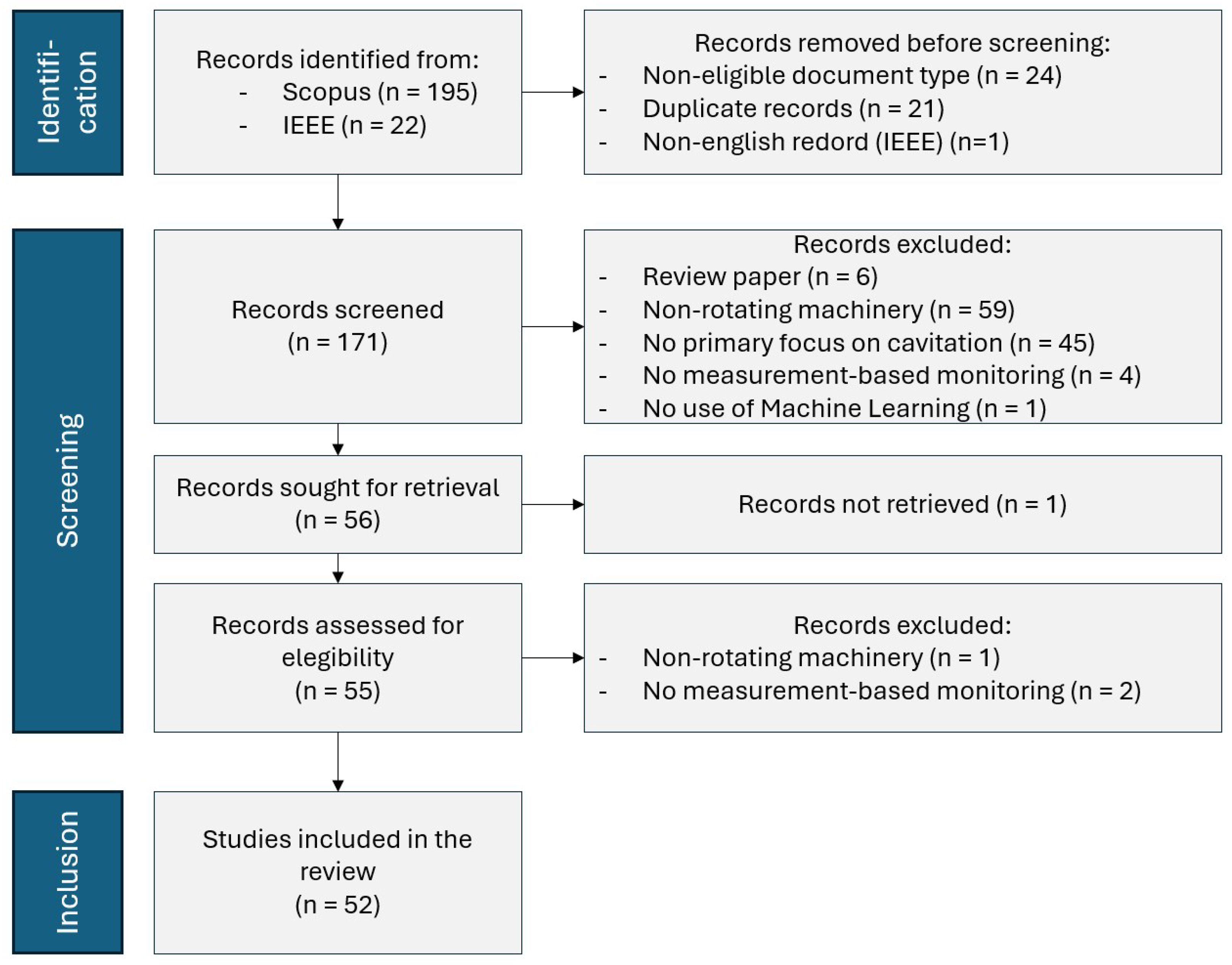
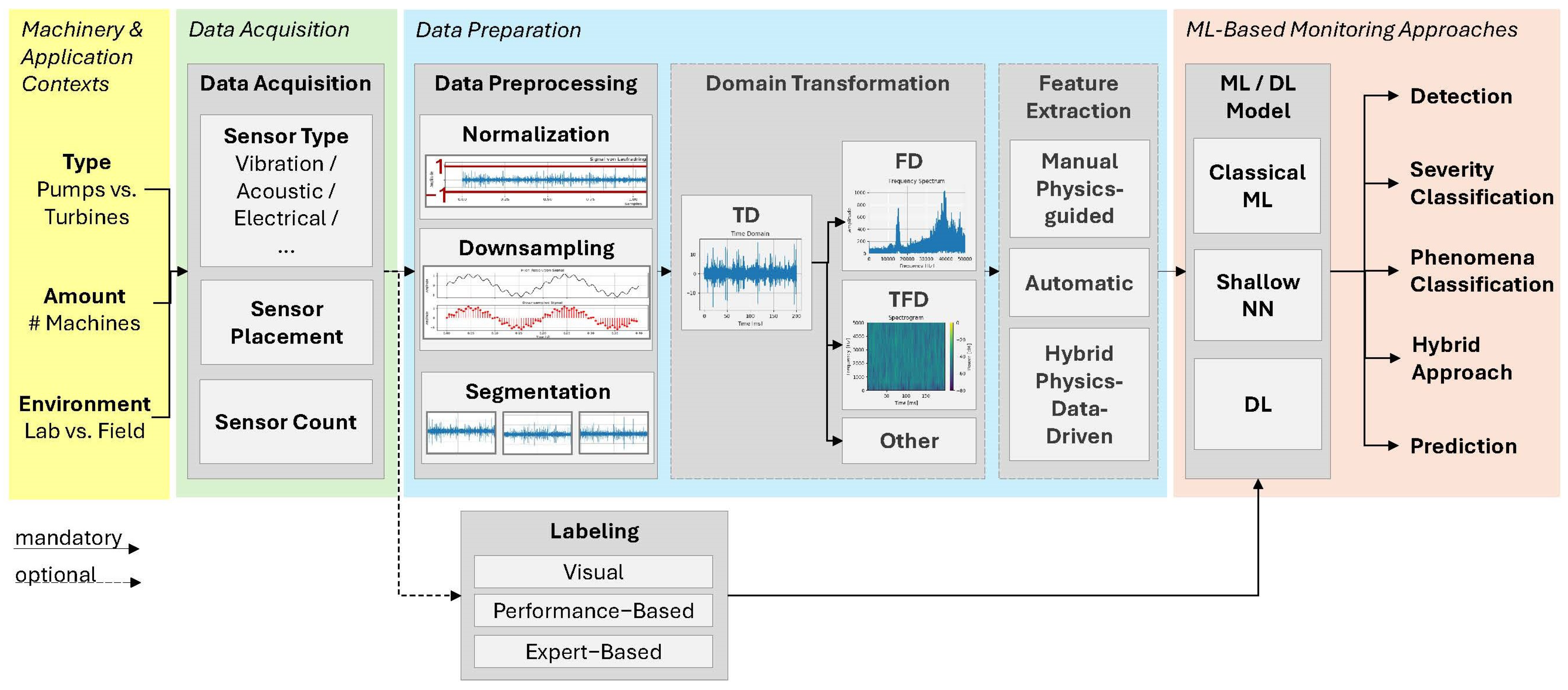
The database searches yielded 217 records (Scopus: n = 195; IEEE: n = 22). After excluding 24 non-eligible document types, 21 duplicates and one non-English IEEE report during identification, 171 records underwent title/abstract screening. From these, 115 were excluded (6 reviews; 59 non-rotating machinery; 45 non-primary cavitation; four non-measurement-based; one non-ML/DL), advancing 56 to full-text review. In the full-text review, one study was excluded because the full texts was not retrievable and three studies were removed for not meeting the PCC criteria (one non-rotating machinery; two non-measurement-based). This resulted in a final sample of 52 studies for analysis (Figure 1) illustrates the PRISMA study selection flowchart from initial records to included studies with excluded records at each stage. The 52 included papers are analyzed in the following chapters, along the ML cavitation monitoring pipeline in Figure 2, which was inductively developed as part of this review. The pipeline synthesizes recurring methodological stages observed across the included studies and abstracts them into a unified, technology-agnostic structure. It spans the progression from system and data context, through data acquisition and processing, to ML-based inference and output definition.

3.2. Machinery and Application Contexts

This subsection provides an overview of the hydraulic machinery types and contexts in the reviewed literature, summarizing investigated machines, assessing per-study machine counts and comparing study environments.

3.2.1. Machinery Types

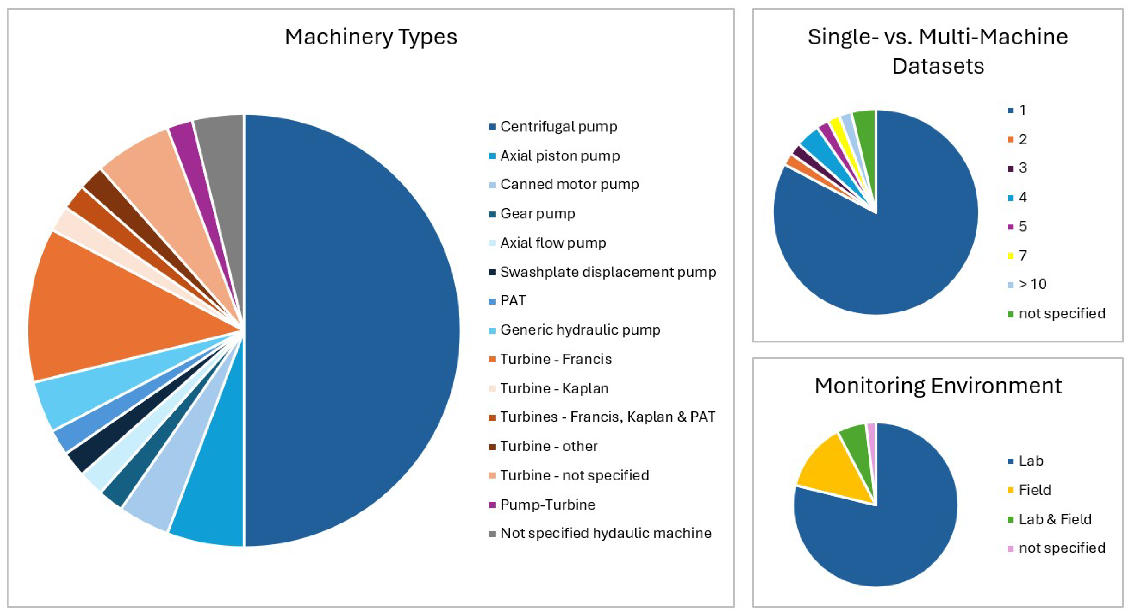
The reviewed studies cover a range of hydraulic machinery types for cavitation monitoring using ML and DL methods, primarily distinguishing between pumps and turbines. Most investigations (26) focus on centrifugal pumps, alongside smaller subsets on axial piston pumps (3 [6,7,8]), canned motor pumps (2 [24,25]), mixed-flow pumps (1 [26]), axial flow pumps (1 [27]), gear pumps (1 [28]), large capacity swashplate displacement pumps (1 [29]) and generic hydraulic pumps (1 [30]). In comparison, approximately one quarter of the studies (12 total) address hydraulic turbines, mainly Francis units (6), with one Kaplan turbine [31], another analyzing Francis, Kaplan and pump-as-turbine (PAT) types [11], one axial flow paddle turbine [32] and three with unspecified turbine types [33,34,35]. One study focuses on PAT systems [12], one analyzes a pump-turbine [36] and one machinery type remains unspecified overall [37].

Across the reviewed studies, this distribution—71% pumps (with centrifugal pumps accounting for 50%) and 23% turbines—highlights a strong bias toward centrifugal pumps over turbines and specialized pump variants. In Figure 3 (on the left), pump-related machinery types are highlighted in blue, while turbine-related variants are shown in orange. This distribution signals the need for expanded ML/DL research on these under-represented types to advance cavitation monitoring (Figure 3).

3.2.2. Single- vs. Multi-Machine Datasets

The majority of studies (83%), as illustrated in Figure 3, focus on a single machine instance (one individual machine unit rather than one machine type), providing in-depth but machine-specific insights into cavitation dynamics and monitoring efficacy. Only a limited number incorporate multi-machine datasets for enhanced generalizability: one study examines two machines (a laboratory model and an operational unit) [38]; another assesses three centrifugal pumps, comparing different ML approaches [39]; two analyze four centrifugal feed pumps in geothermal facilities [14,15]; one evaluates five laboratory turbines [33]; one contrasts ML and DL across seven centrifugal pumps [40] and the largest dataset encompasses 11 machines (six models and five prototypes spanning Francis, Kaplan and PAT configurations) [11]. Two studies omit details on the number of machines being analyzed.

Although several investigations utilize multiple machines, most focus on examination of identical units. Only Gaisser et al. [11] incorporate diverse turbine types (Francis, Kaplan, PAT), underscoring generalization difficulties arising from variations in turbine geometries and sensor configurations.

These findings highlight the need for expanded research employing large-scale, multi-machine and multi-type datasets, since single-machine models, while performant on their training unit, often exhibit poor transferability across heterogeneous hydraulic machinery.

3.2.3. Monitoring Environment

Approximately 80% of the analyzed cavitation studies use lab conditions with test rigs for high-resolution measurements, enabling precise control, cavitation visualization, accurate labeling and robust ML model training/validation (Figure 3). This controlled approach ensures high-fidelity datasets but limits direct applicability to operational field settings.

Combined laboratory-field investigations address the domain shift between idealized lab data and real-world operations by assessing model generalization. For instance, Amini et al. [38] developed an acoustic emission-based ML system on a hydrofoil test rig, attaining over 90% classification accuracy upon validation against operational Francis turbines at the Ernen hydropower plant, despite ambient noise interference. Gaisser et al. [11] applied domain alignment training to a DL model using lab-derived acoustic data, exposing generalization constraints tied to turbine design and sensor placement during multi-turbine field tests. Powar et al. [35] engineered an ML framework trained on simulated lab datasets spanning diverse conditions, yielding 94.2% accuracy in real-time field deployment across varying turbine speeds and flow rates.

Field-only implementations affirm practical viability amid industrial constraints: Cruz Rangel et al. [41] realized non-intrusive cavitation detection through edge computing and motor current signatures. Abrasaldo et al. [14,15] applied semi-supervised ML on geothermal binary plant pump data to uncover 20 undocumented cavitation events. Favrel et al. [42] clustered two years of Francis turbine monitoring data to identify full-load surge regimes and predict onset via ML, achieving 96% accuracy. Zhao et al. [36] validated their DL model on field high-head pump-turbine pressure data, achieving an $R^2$ up to 0.9851 for 50 min cavitation forecasts based on pressure pulsation predictions. He et al. [37] validated their ML model on field vibration data from a Cavitation Warning System on large hydraulic machinery, achieving 98.6% accuracy.

While laboratory environments yield high-fidelity data for ML development, they fail to capture field noise, variability and domain shifts—limiting operational generalization. To urgently shift research focus to field deployment, future research must prioritize mixed lab-field designs, forge industrial partnerships for authentic field data access and develop robust algorithms like domain adaptation and noise-resilient features for real-world variability. This transition is crucial for scalable cavitation monitoring in hydropower.

3.3. Data Acquisition

The reviewed studies use diverse sensing and data acquisition strategies to capture cavitation signatures in pumps and turbines. Vibration and acoustic measurements dominate, typically complemented by process variables to define operating conditions and labels, with data collected mainly under steady or quasi-steady regimes across varying operating points.

3.3.1. Sensing and Signals

Many different sensing and signal processing methods are available for cavitation monitoring. Most studies rely on structure-borne vibration sensing using accelerometers, often complemented by pressure [13] and flow measurements [7] or motor current signals [43] to characterize operating conditions and detect cavitation. For instance, DeSouza et al. [13] integrate vibration spectra with pressure coefficient data to improve cavitation detection in Francis turbines. Acoustic sensing is also common, using water-borne hydrophones (e.g., [34,44]), airborne microphones (e.g., [38,45]) or structure borne acoustic emission sensors [11]. Measured acoustic emission (AE) ranges span from the audible regime (e.g., [38,44]) to ultrasonic frequencies up to 2 MHz [9,11,33]. Hybrid schemes, as used by Gruber et al. [9], that combine the vibration and acoustic techniques are adopted to enhance diagnostic coverage and reliability. Zhang et al. [46] showed that their ML model achieved the highest accuracy of 99.17% in recognizing noise signals under cavitation states, followed by vibration signals at 98.89%, with pressure pulsation signals lowest at 81.67%. A smaller group of studies employs hydraulic process parameters—such as flow rate, speed, torque, suction head and delivery head—alongside acoustic signals like noise [47], while others incorporate electrical sensors (e.g., voltage, current) and mechanical measures like shaft displacement [42,43] to build multimodal datasets enhancing ML performance. Other studies use electrical signals. For instance, Won [48] demonstrated non-intrusive incipient cavitation detection in pumps using 500 Hz motor current signals. Cruz Rangel et al. [41] proposed a load monitoring method using current signals to detect cavitation in HVAC pumps under variable speeds. Hu et al. [49] developed a low-cost IoT system with Arduino-integrated voltage sensing for cavitation detection.

Complementary investigations have examined the influence of operating parameters and the integration of physics-informed learning. Song et al. [16] observed a strong dependence of cavitation phenomena on rotational speed, with temperature exerting only a minor influence. Wang et al. [7] used the Temporal–Spatial Method of Characteristics (TSMOC) to reconstruct pump flow ripples from pressure data, combined with domain-adapted transfer learning (DPAM-CORAL). This achieved 98% accuracy in classifying cavitation intensity across varying conditions.

For field applications, low-cost sensing has proven particularly attractive. Hu et al. [49] reported 99.47% classification accuracy using MEMS accelerometers within an IoT architecture, while Arendra et al. [50] achieved 82.5% accuracy employing low-cost microphones combined with Articifical Neural Network (ANN)-based classification. Karagiovanidis et al. [51] further extended this paradigm by demonstrating smartphone-based cavitation monitoring using built-in accelerometer and microphone sensors, where vibration—particularly x-axis components—outperformed acoustic signals under field conditions. Collectively, these findings validate the feasibility of affordable and portable sensing solutions for real-time cavitation detection in industrial environments.

It can be identified that vibration sensing via accelerometers predominates for pumps, while acoustic signals are favored for turbines, though both modalities appear across applications. This trend reflects differences in signal propagation and erosion-monitoring priorities. Across the reviewed studies, sensor selection remains largely empirical, with no consistent guidance for choosing or combining modalities based on objectives or constraints—a gap that points to an important direction for future research. Sampling rates are tailored to the signal characteristics: typically 100 s of Hz for process parameters (e.g., flow, pressure), 10 s of kHz for vibration/audible acoustics and MHz for ultrasonic acoustic signals to resolve transients. Low-cost, non-intrusive electrical sensing (e.g., motor current) emerges as promising for scalable diagnostics. Future efforts should compare AE against accelerometers for detection efficiency [13] and advance physics-informed multi-sensor fusion [9] integrating operating conditions to boost reliability and cross-scenario generalizability.

3.3.2. Sensor Placement

The studies reveal distinct patterns by sensor type for cavitation monitoring, with lab setups enabling precise near-source placements and field installations favoring non-invasive external mounts [11]. Vibration accelerometers are usually mounted on the pump casing [52], bearings [24] or turbine casing [35]. Acoustic sensors show greater variability but favor locations near the draft tube [9,34] and airborne microphones close to casings or cavitation sources [50]. Pressure transducers often cluster at suction/delivery ends (pumps) [47] or draft-tube/spiral-casing walls (turbines) [42,53], sensitive to cavitation-induced instabilities. Electrical sensors (current/voltage) integrate into motor drives [30]. Nasiri et al. [54] offer simple guidelines for placing vibration sensors to detect cavitation in centrifugal pumps using neural networks. With one sensor, place it radially for basic detection. Two sensors work best as radial plus back to cut errors. Three sensors—radial, back and front—are suggested to obtain perfect, error-free results. Overall, no universal location emerges across types, but near-field hydraulic regions (impeller channels, draft tubes) and structural paths (casings, bearings) dominate.

3.3.3. Sensor Count

Sensor configurations in cavitation monitoring range from single-sensor setups (e.g., [31,55,56]) to arrays of up to eight accelerometers [4,24]. A clear distinction must be made between multi-sensor arrays of the same modality (e.g., several accelerometers measuring vibration at different locations) and multi-modal sensor systems combining different physical principles (e.g., vibration, acoustic emission, electrical current).

For homogeneous multi-sensor arrays, the primary benefit lies in improved spatial coverage and reduced sensitivity to local mounting effects. However, the literature does not support a consistent “more sensors → better model” relationship. Multiple sensors of the same type often provide redundancy rather than additional information and carefully positioned single-sensor systems can achieve comparable performance when labeling quality is reliable.

By contrast, substantial gains arise from multi-modal sensor fusion, which integrates physically complementary signals. Song et al. [43] report an increase in recognition accuracy from 73.9% (current) and 89.3% (vibration) to 97.3% when both modalities are fused. Similarly, Dong et al. [5] show that inception-stage detection improves from >80% (single sensor) to >99% (two modalities) and 100% (≥3 modalities). These findings indicate that performance improvements primarily stem from complementary physical information rather than increased sensor count alone.

3.3.4. Operating Regimes

Operating regimes refer to defined, steady-state combinations of pump or turbine parameters—such as rotational speed, flow rate, head or net positive suction head and load—that generate distinct cavitation conditions during signal acquisition. These representative regimes are deliberately selected to enable controlled labeling of cavitation states.

The operating regimes are commonly established through parametric variation of individual operating variables, including rotational speed via motor control [28], flow rate via discharge valve adjustment [5,43,44] and NPSH via suction throttling [4,25,57,58]. Several studies extend this approach to multi-dimensional parameter spaces, for example combining speed and flow [47], speed and pressure [7] or flow and NPSH [24], thereby capturing a broader range of cavitation regimes.

Such systematic parameter control is primarily feasible in laboratory environments, where operating conditions can be deliberately imposed and held constant. In contrast, field data from real operation are subject to operational constraints, grid demands and environmental variability, limiting the ability to define and reproduce clearly separated regimes for model training.

The number of investigated operating regimes varies considerably across studies, ranging from 2 to 297 (median ∼4) and typically encompassing 2–4 cavitation severity levels. Won et al. [48], for example, created binary cavitation/no-cavitation regimes by injecting air bubbles to simulate cavitation (vs. normal operation). Experimental designs extend from simple binary cavitation/no-cavitation classifications to dense parametric grids, such as 30-point matrices (3 flow rates × 10 NPSH values [24]) or large-scale campaigns with 297 operating points [40]. Despite this numerical variability, the underlying design philosophy is often similar: many studies rely on a limited set of clearly separated steady-state conditions, frequently selecting a single representative regime per class. Only a few investigations systematically explore continuous or densely sampled operating spaces. Furthermore, most experiments are conducted under step-wise transitions between steady regimes, whereas genuine transient dynamics, such as valve closure sequences [59] or start/stop ramping [38], remain comparatively underrepresented.

Future research should therefore prioritize broader, multi-dimensional and dynamically varying coverage of the operating domain. Incorporating continuous parameter variations and transient conditions would enable smoother decision boundaries, improve model robustness and enhance generalization to real-world operation, where operating points evolve continuously rather than transitioning discretely between a limited number of predefined steady-state regimes.

3.3.5. Labeling Strategies

Labeling involves assigning class identifiers (e.g., none, mild, severe) to measured signals to establish ground truth for supervised ML models. Reliable labeling is crucial, as it allows models to learn discriminative patterns and enables validation against physically meaningful operating states. Labels are typically derived from physical indicators, visual observations or expert interpretation, with reliability depending on experimental control and direct reference evidence.

Visual labeling: This approach delivers high-quality ground truth in laboratory setups via transparent casings and high-speed imaging, enabling direct cavitation observation for unambiguous class definitions. Techniques encompass void fraction via edge detection [53], stroboscopy [34,54], bubble density analysis [26], manual auditory–visual verification with videos [38], vortex detection in camera images [60], transparent housing with optical sensors [52,55], pixel-counting intensity quantification [4] and high-speed monitoring of impeller outlets or passage bubble counts [16,26].

Performance-based labeling: This method indirectly infers cavitation severity via standardized NPSH and head-drop thresholds (e.g., [5,45,61]), cavitation numbers from experts [62], volumetric loss coefficients [6,7], valve positions inducing cavitation [49,51,57] or manufacturer curves. While reproducible, especially the NPSH-based head-drop criteria method reveals inconsistencies, as stage definitions vary across studies (

Table 1. Head-drop thresholds for cavitation stages across studies.

Study	No Cavitation	Incipient	Obvious	Severe
[44]	<1%	1–3%	–	>3%
[58]	<1.5%	1.5–3%	–	>3%
[57]	<3%	3–6%	–	>6%
[45]	<1%	1–3%	3–5%	>5%

). Incipient cavitation typically occurs at 1–3% head drop and severe at >3–6%, though visual onset often precedes measurable drops—necessitating context-specific criteria for reliable ML labeling. Furthermore, Tong et al. [4] quantified cavitation intensities using a pixel-counting method as ratio of cavity region to flow passage between adjacent blades and showed that actual cavitation occurs at 42.1% head drop, exceeding the 3% threshold.

Hybrid approaches combine methods for robustness, such as valve opening with stroboscopic bubble observation [54], 3% head loss with high-speed photography [43] or sequential visual/sound inspection, pressure coefficient deviations and vibration spectra peaks [13].

Field- and expert-based labeling: Predominant in field operations, this strategy relies on operator judgment, maintenance records and manufacturer charts. Examples include expert spectral clustering using criteria like fundamental frequency [42], powerplant expert knowledge [38] and operator-documented events with semi-supervised validation [15]. Unlike lab methods with visual or NPSH linkages, field labeling risks noisy annotations, causing models to capture plant-specific artifacts over genuine cavitation signatures. Field data further suffer label scarcity from costly annotation and operational variability, necessitating unsupervised clustering of unlabeled signals [41,42] and semi-supervised extension of sparse expert labels [14].

While existing approaches suffice in controlled settings, inconsistent labeling—especially varying head-drop thresholds (e.g., 1–3% vs. 3–6% incipient; Table 1)—hinders ML reproducibility, training (blurred boundaries) and field generalization. Standardized physics-based criteria, such as IEC-aligned NPSH_3% (3% head drop) margins or community benchmarks, would enable fair cross-study validation. Additionally, further research should prioritize semi-supervised architectures to bridge lab-field gaps for generalizable hydropower monitoring.

3.4. Data Preparation

The reviewed studies apply a wide range of data preparation strategies, spanning from minimal preprocessing of raw time-series to heavily engineered pipelines combining signal conditioning, domain transformations and feature extraction. Depending on the chosen approach, cavitation-related information is either explicitly enhanced through physics-guided signal processing or implicitly learned by data-driven models from high-dimensional signal representations.

3.4.1. Data Preprocessing

Most studies perform basic signal conditioning prior to model training to improve robustness and comparability across sensors, operating points and machines. Common steps include resampling, normalization—predominantly to zero mean and unit variance—and segmentation (e.g., [26,40,61]). These operations aim to suppress sensor-specific artifacts, reduce redundancy and stabilize the numerical optimization of ML and DL models, particularly when combining data from multiple operating regimes or measurement campaigns.

3.4.2. Signal Analysis Domains and Transformation Methodologies

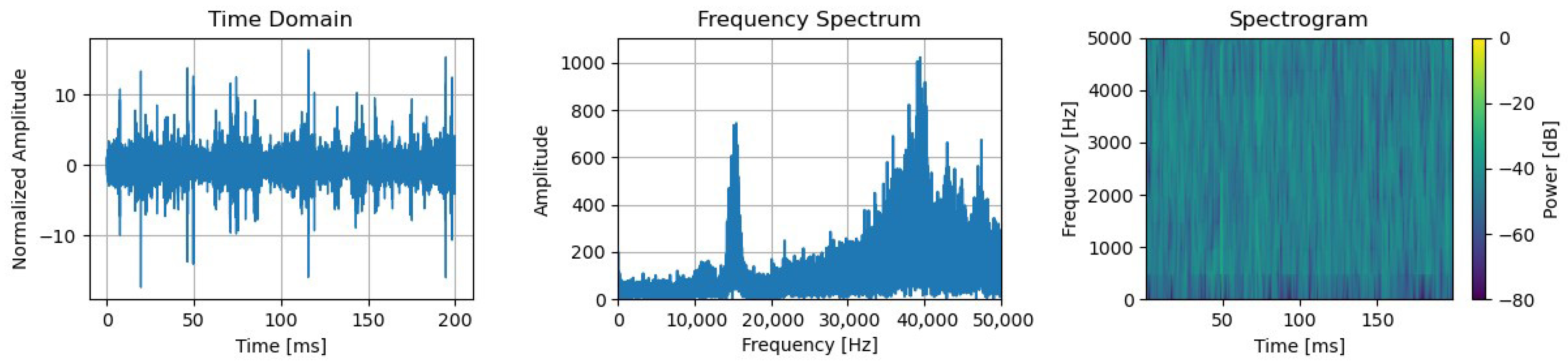
Signal analysis domains provide alternative mathematical representations of raw sensor data to reveal hidden cavitation patterns invisible in time series. While the time–domain (TD) signals capture raw temporal dynamics, frequency–domain (FD) representations reveal periodic components via spectral analysis and time–frequency domain (TFD) methods track evolving frequencies. A comparison of the three domains can be seen in Figure 4. While optional—since raw time–domain signals can be fed into models directly—domain transformation is widely used to amplify cavitation signatures before learning.

TD signals are routinely converted to FD via the fast Fourier transform (FFT) [26,51,54] and TFD via the short-time Fourier transform (STFT) [6,24,33,37] or the continuous wavelet transform (CWT) [35,45]. Less common are the correlation domain [9] and spatial domain [49] mapping which further reveal statistical dependencies and cavitation propagation across sensor arrays, respectively.

In addition, adaptive decomposition techniques such as wavelet packet decomposition (WPD) [5], empirical mode decomposition (EMD) [7,55] and variational mode decomposition (VMD) [25,36,57,62] are employed to separate oscillatory components and isolate frequency bands associated with bubble collapses and flow instabilities. These transformations are motivated by cavitation physics, as cavitation-induced broadband noise, sidebands and amplitude modulations are often more distinguishable in spectral or time–frequency representations than in raw time-series.

While basic FFT/STFT methods are prevalent, advanced techniques demonstrate superior performance. Wu et al.’s [24] time–frequency analysis (TATF) applies time-synchronous averaging to suppress noise in periodic pump vibrations before time–frequency analysis, outperforming STFT and wavelet transforms across signal-to-noise-ratio (SNR) levels. Sun et al.’s multi-adversarial attention network (MAAN) uses a novel residual convolutional attention feature extractor with a Multi-Scale Global Hybrid Attention Module (MSG-HAM) to enhance CWT features with multi-adversarial alignment, achieving >93% accuracy across 12 tasks by addressing domain shift, making it suitable for variable pump operations [45].

In summary, domain transformations are widely used to enhance cavitation-related features, with frequency- and time–frequency-based methods predominating. While FFT and STFT remain standard, adaptive and advanced techniques show improved robustness and sensitivity. Future research should therefore explore physics-informed transformation that explicitly incorporate cavitation dynamics to improve interpretability, robustness and generalization.

3.4.3. Feature Extraction Strategies

Feature extraction transforms raw sensor signals into compact representations that capture cavitation-relevant characteristics. By summarizing statistical, spectralor structural properties, it reduces dimensionality and highlights discriminative patterns. This improves interpretability, computational efficiency and robustness, particularly when data are limited or noisy. In the reviewed literature three principal feature-extraction paradigms can be identified.

Physics-guided manual feature engineering: This paradigm relies on manually designed, physics-informed descriptors extracted from time, frequency and time–frequency domains. Common features include statistical measures (RMS, skewness, kurtosis, crest factor, entropy) [8,35,43] and spectral peaks [12,41,42], which are subsequently used in classical ML models. This approach offers interpretability and moderate data requirements. Even minimal sets can suffice: Gruber et al. [9] achieve robust classification using only three features—mean amplitude, coefficient of variation and cross-correlation distortion. Azizi and Demir [55] used Bees Algorithm-optimized hybrid feature selection (filter-wrapper) to reduce 90 features to <4, achieving 100% accuracy across ANN models for cavitation severity. Fu et al. [32] fuse time/frequency health indices (RMS, kurtosis, etc.) via interpretable logistic weights for turbine cavitation detection. Feature extraction is often preceded by adaptive decomposition to isolate informative components. Hajnayeb and Ghasemi [52] compare discrete wavelet transform (DWT), EMD and Ensemble-EMD (EEMD) for General Regression NN-based diagnosis, extracting five statistical features from selected intrinsic mode functions (IMFs) and identifying the first two (DWT) and four (EMD) IMFs as most diagnostic, with DWT being more efficient. Similarly, Dong et al. [44] use WPD to select high-energy bands and combine frequency-division statistics with PCA, achieving 98.2% accuracy. Other studies apply FFT-based correlation analysis for feature selection [50], multi-domain statistical extraction [8,59] or automated frameworks such as tsfresh for semi-supervised detection [15]. Carefully engineered features can rival deep models: Hu et al. [49] report 99.47% accuracy using Hu’s Moments with k-NN, outperforming DenseNet169 and ResNet50. Robustness is further enhanced through multi-domain strategies and mechanism-guided selection, as demonstrated by Song et al. [58] and Azizi and Demir [55].

Automatic feature learning via deep architectures: The second paradigm comprises automatic feature learning via DL architectures, which learn task-specific filters and hierarchical representations directly from raw or minimally processed inputs, reducing reliance on expert-defined indicators. Tan et al. [26] achieve 87.2% accuracy for mixed-flow pumps using a convolutional neural network with batch normalization and a multilayer perceptron classifier (CNN-BN-MLP) with FFT-transformed signals and bubble-density labels from high-speed photography. Song et al. [16] propose a demodulation-efficient network (DEN) extracting modulated frequencies via signal demodulation into EfficientNet, achieving 89.44% accuracy across varying temperatures/frequencies, outperforming FFT inputs by 20.69% and autoencoders by 25.28%. Kang et al. [31] apply stacked sparse autoencoder (SSAE) for unsupervised pre-training.

Hybrid physics–data-driven feature learning: The third paradigm encompasses hybrid pipelines that combine physics-inspired preprocessing with data-driven learning, aiming to inject physical insight at early processing stages while exploiting the flexibility of automatically learned features at higher abstraction levels. Examples include transform-based decompositions followed either by manual statistical selection [44] or by deep networks for subsequent representation learning. For instance, Li et al. [25] decompose the signals using variational mode decomposition (VMD), select relevant modes based on entropy criteria and feed them into an attention-enhanced deep convolutional neural network incorporating a convolutional block attention mechanism, attaining 99.66% accuracy across four operating states. Chao et al. [6] train a CNN on STFT spectrograms, generate Grad-CAM masks for denoising and re-train—boosting noisy accuracy from 50% to 89% (SNR = 4 dB). Yu et al. [27] decompose pressure signals via VMD + sample entropy, then apply SWO-optimized BiLSTM for continuous cavitation coefficient identification (<5% MAPE). Wu et al. [24] employs time synchronous average + time–frequency analysis (TATF) via STFT on time synchronous averaging (TSA) matrix after principal component analysis (PCA). Zhang et al. [46] use STFT+PCA for 2D eigenmatrices and FFT spectra from multi-sensor signals, fused via 1D/2D CNNs before ConvGRU classification (>98% accuracy).

The literature exhibits a clear evolutionary trajectory from manual physics-guided engineering toward automatic ML, with hybrid pipelines emerging as the dominant paradigm to reconcile interpretability with performance.

3.4.4. Signal Representation

Signal representation defines how sensor data are presented to ML models—ranging from raw time-series and extracted scalar features to 2D spectrograms—shaping model choice, computational load and cavitation detection performance.

End-to-end learning directly feeds near-raw time-series into deep models [4,28], enabling automatic feature discovery and site-specific adaptation, though larger datasets and careful regularization are required. For instance, Siano et al. [28] detect cavitation from sub-rotation vibration segments in real time and Tong et al. [4] classify eight cavitation states with >95% accuracy using multi-channel raw vibrations.

TD and FD features are typically represented as 1D vectors of scalar statistics—such as RMS, spectral peaksor energy [38,54,63]—or, in some cases, as 2D feature matrices [27]. These compact representations interface naturally with classical ML algorithms, offering interpretability and moderate computational demands. Their simplicity supports small-to-medium datasets and facilitates understanding of which features drive cavitation detection, though they may limit expressive power and sensitivity to subtle nonlinear patterns.

Time–frequency domain transformations produce 2D image-like representations—STFT spectrograms [11,33,37], wavelet scalograms (CWT) [45], bispectrum maps [56] or demodulation spectra [16]—enabling CNNs to exploit translation-invariant time–frequency patterns. Such representations capture complex cavitation stages and nonlinear effects directly from raw signals [49,56], at the cost of higher data and computational demands and reduced interpretability. Zhang et al. [46] conclude that PCA on time–frequency analysis best distinguishes cavitation states in vibration signals, outperforming time/frequency domains.

The choice between raw signals, numerical vectors or spectral images reflects a trade-off between interpretability, data availability and representational power, motivating the need for systematic selection criteria and standardized benchmarks.

3.5. ML-Based Monitoring Approaches

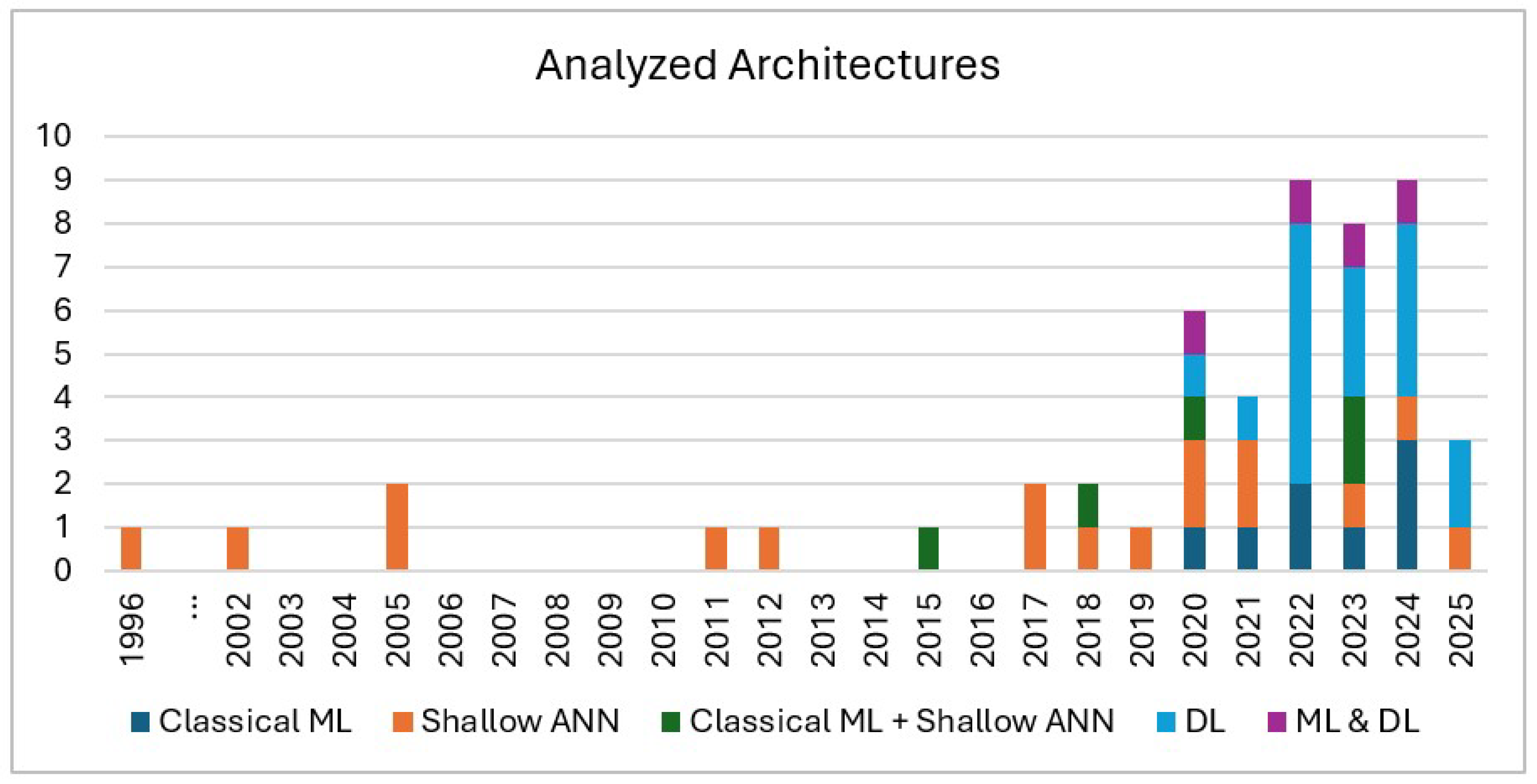
Over the last five years, research activity regarding cavitation monitoring via ML has accelerated, with DL methods enabling largely automated feature extraction and high-fidelity detection, while classical ML approaches remain relevant for their interpretability and lower data demands. Figure 5 illustrates the steady rise in data-driven cavitation studies over the last decade, highlighting the transition of ML- and DL-based monitoring from a niche topic to a rapidly growing field.

Correspondingly, the reviewed literature demonstrates that cavitation in hydraulic machinery is now addressed using a diverse spectrum of data-driven approaches, differing in task formulation, model families and the degree to which they rely on expert-defined versus autonomously learned representations.

3.5.1. Monitoring Objective

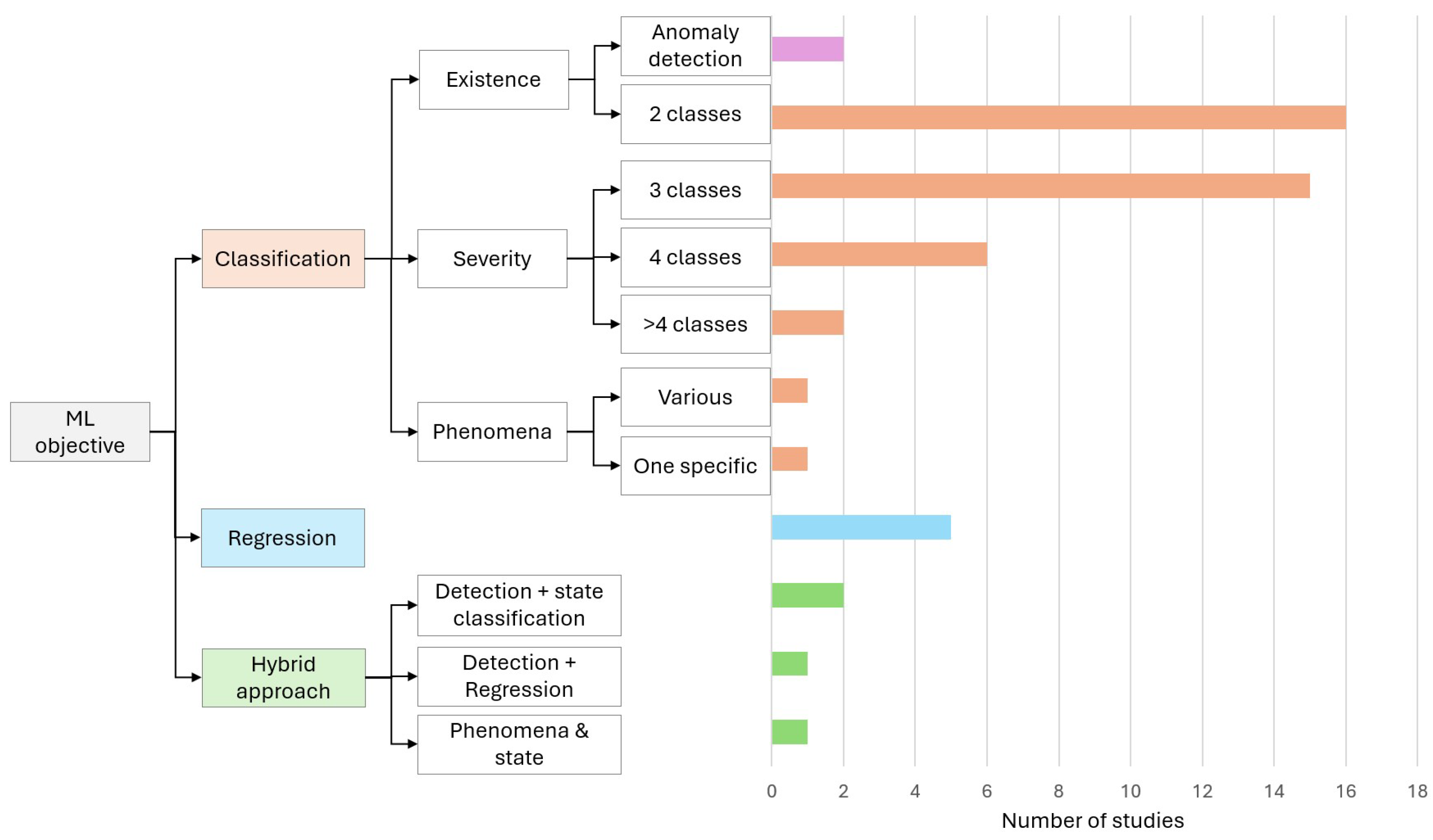
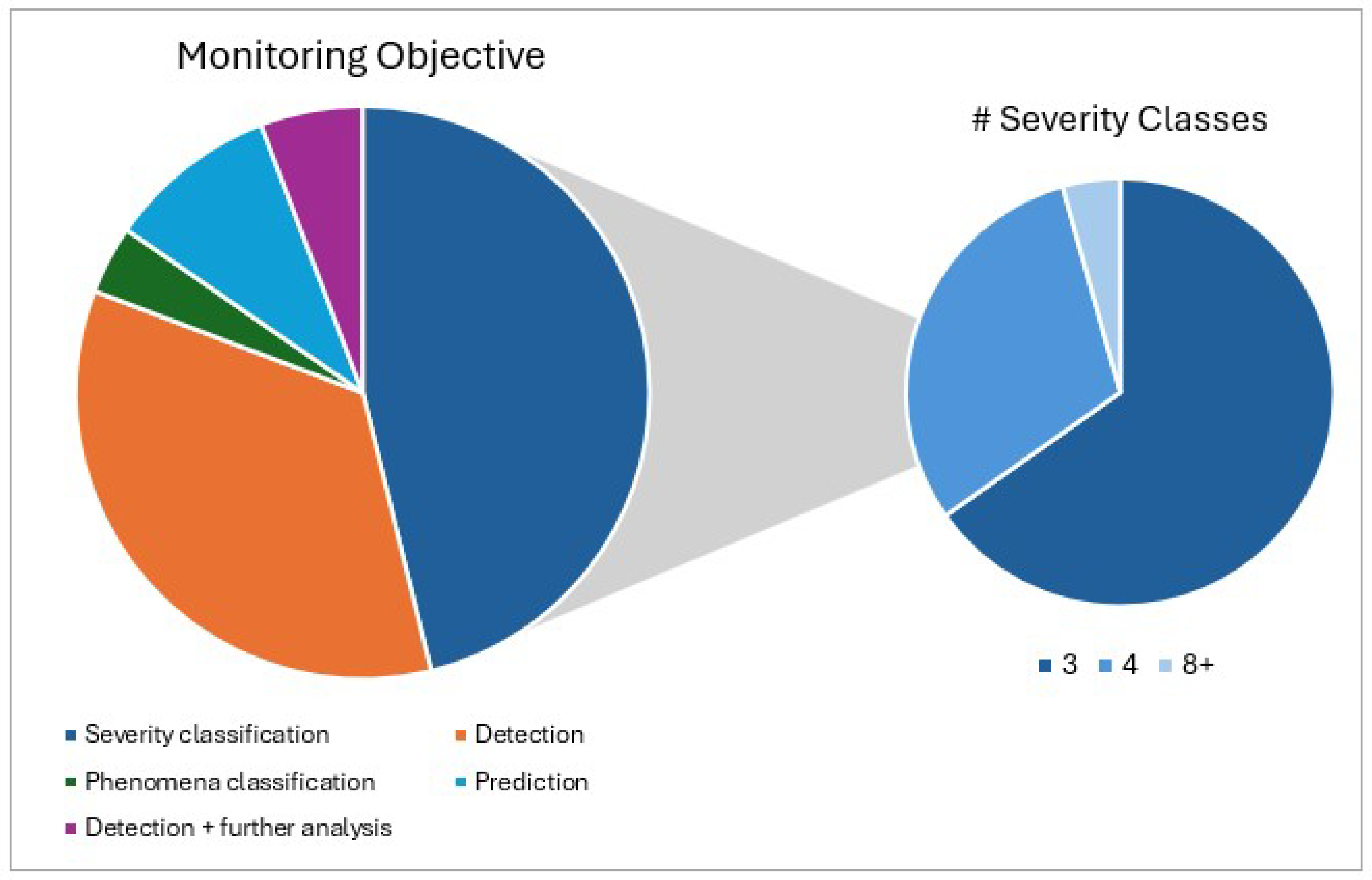
The monitoring objectives in the reviewed work can be grouped into four main categories, with a few hybrid formulations spanning more than one group (Figure 6). Most papers either treat cavitation as a binary fault (existence), resolve multiple discrete severity states, classify phenomena or predict continuous indicators that reflect cavitation intensity more gradually. Figure 7 expands on Figure 6 with a hierarchical tree and study counts, revealing a strong focus on binary existence detection (14 studies) and 3-class severity classification (15 studies). The four objective categories are outlined in detail below.

• Detection: A substantial share of studies (e.g., [11,32,33,35,62]) formulates cavitation monitoring as a binary classification task, where models decide whether cavitation is present or not. These two-class detectors are attractive for real-time protection and alarm systems, as they are simple to train, require fewer labeled regimes and can generalize reasonably well across operating points when trained on representative normal and cavitating data. Their main limitation is the lack of information on cavitation severity or mechanism, requiring additional logic for maintenance prioritization and efficiency assessment.
  Anomaly detection represents a special case of binary detection: models are trained only on normal operating data and flag deviations as potential cavitation or surge events [28,41]. This unsupervised approach can detect unforeseen or rare cavitation patterns without explicit labeling, though it does not distinguish between different types or intensities of cavitation.
• Severity classification: The multi-class setting is the dominant objective overall and mostly used for severity classification, where models distinguish several discrete regimes. The majority of the multi-class studies considers 3–4 classes—mostly distinguished in “no cavitation”, “incipient cavitation”, “severe or fully developed cavitation” (e.g., [5,8,52]), some also including “moderate cavitation” as a fourth class (e.g., [6,7,25]). These discretizations, however, prove inherently limited: states just below/above boundaries are often more similar than distant intra-class points, blurring decision margins. Two works therefore define finer grids with up to 10 classes (operating states) [4,51] to track gradual cavitation evolution and support operating-point optimization rather than simple fault/no-fault decisions. Furthermore, classification depends on thresholds, as Won et al. [48] showed (NN accuracy dropping from 100% at thr = 0.05 to 87.5% at thr = 0.01 Euclidean distance).
• Phenomena classification: Most studies treat cavitation in a binary way or categorically (none/mild/severe), rarely linking types to sensor signatures. However, each type has unique acoustic/vibration characteristics—directly influencing ML feature design—e.g., sheet cavitation (slight pulsation); cloud cavitation (strong oscillations, pulsating behavior); interblade vortex (high broadband noise); traveling bubble (high-frequency pulses) and vortex (low-frequency pulses) [10]. Only a small subset of studies employs phenomenon-level classification. Gruber et al. [9] distinguish normal operation from cavitation types (four classes: pure water, draft-tube swirl, interblade vortex, leading-edge cavitation), while Favrel et al. [42] focus on one specific phenomenon, classifying three surge types.
• Prediction: A third category addresses prediction, treating cavitation intensity as continuous by regressing e.g., void fraction [53], damage area or hydraulic metrics [47]. Hočevar et al. achieve R² = 0.82–0.98 predicting Francis turbine void fraction from pressure fluctuations using a radial basis neural network (RBNN) [53]. Stephen et al. [47] predict total head, NPSH, efficiency and noise in a low-specific-speed centrifugal pump using random forest and extreme gradient boosting on inputs like flow rate, speed, torque, suction head and delivery head, achieving correlation coefficients near 1 for hydraulic metrics (except noise). Yu and Cheng [27] regress cavitation coefficient $\sigma$ in axial flow pumps from VMD-decomposed pressure signals using a SWO-BiLSTM. Zhao et al. [36] forecast pressure fluctuations in high-head field pump-turbines using VMD-DBO-GRU-Attention (50-min ahead). Orhan et al. [61] regress NPSH_3% cavitation threshold, noise and vibration in radial pumps via ANN/DTR (R² = 0.86).
• Hybrid approach (detection + further analysis): Some hybrid formulations combine the above named objectives, for example, first using a binary classificator to decide whether cavitation is present and then applying a separate multi-class severity model [34,56] or the cavitation amount [40], thereby balancing detection robustness with richer diagnostic information.

The cavitation detection literature shows one trade-off: binary methods are simpler and more accurate (e.g., Kang et al. [34] achieved 93.18% with stacked sparse autoencoders vs. 71.88% for three-class), while multi-class and regression provide detailed severity insights at higher complexity. Future research should prioritize regression-based continuous severity metrics to resolve boundary ambiguities and enhance remaining useful life precision, alongside phenomenon-focused models that localize specific cavitation mechanisms.

3.5.2. ML Architectures

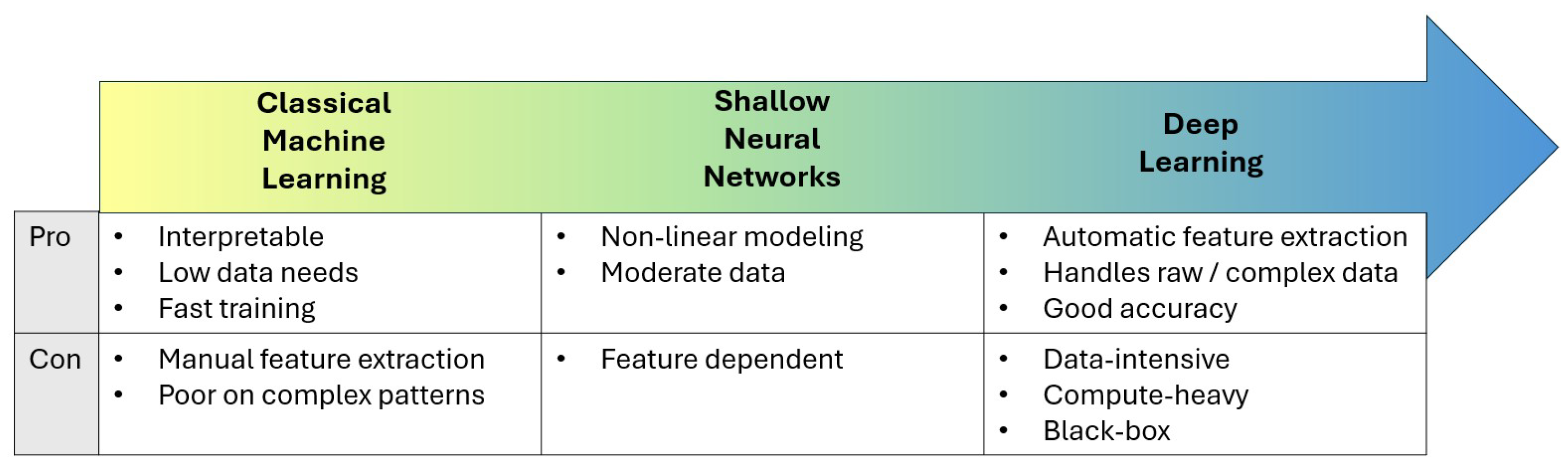
The reviewed work shows a clear evolution from classical ML models, through simple NN, towards more complex DL architectures (Figure 8), each stage offering specific advantages and drawbacks for cavitation monitoring.

Classical ML: Classical ML methods remain prevalent in cavitation detection, particularly due to their interpretability and suitability for limited datasets. The most commonly used models are Support Vector Machines (SVM) [12,14,39,40,43,47,49,51], k-Nearest Neighbors (kNN) [38,39,49,51], Decision Trees (DT) [9,12,35,51], Random Forests (RF) [14,47,49], gradient-boosting [8,14,35,47], linear regression [47], logistic regression [32], Bayesian networks [41], Gaussian Naive Bayes [49] and Gaussian Mixture Models [38] trained on carefully engineered feature vectors derived from the input signals. All these methods exhibit some key trade-offs: they require minimal training data, enable feature-level interpretability linking physical phenomena to predictions, yet depend heavily on expert-designed preprocessing and may fail to capture complex spatio-temporal patterns when the feature space is incomplete. Empirical comparisons reveal method-dependent performance. Dutta [39] demonstrated that SVMs outperform kNN for cavitation detection in real-time pumping systems with limited samples, whereas kNN becomes viable when training samples exceed feature dimensionality. Similarly, Stephen et al. [47] benchmarked RF, SVMs, XGBoost and linear regression on centrifugal pump cavitation data, finding that RF and XGBoost achieved near-perfect correlation for head, NPSH and efficiency predictions, though cavitation noise dynamics remained poorly predictable across methods. Ensemble and hybrid approaches enhance detection performance. Powar et al. [35] report that DT and gradient boosting ensemble achieved 94.2% accuracy in real-time field validation. Similarly, Kang et al. [34] developed stacked sparse autoencoders for unsupervised feature learning from frequency-transformed signals, paired with minimum redundancy maximum relevance (mRMR) selection and RF fine-tuning to boost incipient cavitation detection under varying operating conditions [34].

Shallow NN: As data volumes and computational resources have increased, shallow neural network architectures have become prevalent. Multilayer perceptrons (MLPs) dominate this category [9,12,13,29,42,43,48,49,50,54,55,63], alongside radial basis function (RBF) networks [5,13,44,52,53] and more specialized architectures like a NonLinear AutoRegressive (NLAR) approach [28]. These networks model nonlinear relationships on expert-engineered features, offering greater flexibility than classical ML while integrating into existing monitoring systems, yet remain constrained by input quality and cannot inherently address domain shift between machines.

Early work by Steele et al. [29] showed that MLPs (3–4 hidden nodes) outperforms the fisher linear discriminant, a statistical method. Comparative studies of classical ML and shallow NNs reveal complementary strengths: Stephen et al. [12] found decision trees excel in interpretability while ANNs achieve superior precision (99.86%), proposing a hybrid framework combining both for interpretable and accurate pump-as-turbine classification. DeSouza et al. [13] validated MLP and RBF networks achieving up to 100% and 95.3% accuracy, respectively, for cavitation identification in Francis turbines, with MLPs showing superior generalization to unseen data while RBFs train faster.

Deep Learning: Deep learning has established itself as the leading paradigm in cavitation detection, enabling automatic feature extraction from raw signals and robust performance in realistic scenarios characterized by sparse labels and partial observability. These methods trade interpretability and data efficiency for superior handling of complex, non-stationary signals, requiring larger datasets, careful regularization and substantial computational resources.

Core architectures and variants: Foundational DL architectures process raw time-series or time–frequency representations directly for end-to-end feature extraction: convolutional neural networks (CNNs) capture spatial patterns in spectrograms [40,51], long short-term memory networks (LSTMs) model temporal dynamics [26,27], gated recurrent units (GRUs) and convolutional GRUs (ConvGRUs) capture sequential dependencies in non-stationary cavitation signals [36,46], autoencoders enable unsupervised representation learning [26,58] and transformers leverage attention for long-range dependencies [37]. Tan et al. [26] demonstrated CNN superiority (87.2% accuracy) over stacked autoencoders and LSTMs for multi-level cavitation diagnosis using FFT-transformed vibration signals. Zhao et al. [36] combined variational mode decomposition with dung beetle optimization, GRU networks and an attention mechanism for field pump-turbine pressure forecasting (R² = 0.9851). Advanced variants extend these foundations. CNN architecture modifications include ResNet [11], AlexNet [56], GoogleNet [56], LeNet-5 [6], adaptive NNs (a compact CNN) [4]. Autoencoder variants encompass stacked sparse autoencoders (SSAE) [31], stacked denoising autoencoders (SDAE) [58], artificial immune networks and deep embedding networks (DENs) [16]. Song et al. [58] achieved over 98% accuracy using risk-informed model evaluation (RIME)-optimized SDAEs via automated hyperparameter tuning. Other specialized architectures include adaptive neuro-fuzzy inference systems for real-time vortex cavitation detection [60], early ordered neural networks for multi-level severity monitoring [30] and multi-adversarial attention networks (MAANs) extended with class-aware guidance for domain adaptation across variable pump operations [45]. Bio-inspired optimization further enhances performance: Lang et al. [57] developed an improved Lévy-flight bat algorithm-optimized Elman networks surpassing particle swarm optimization variants, while Matloobi et al. [59] applied artificial immune networks (AINs) holistically from data preparation to early-stage cavitation classification.

Performance comparison DL and ML: DL frequently achieves superior accuracy in cavitation detection, though performance gains depend on dataset size, feature engineering quality and application-specific constraints. Hasanpour et al. [40] validated both SVM and CNN models while notably testing deployment on embedded industrial hardware, bridging algorithmic development with practical implementation. Azizi et al. [55] compared generalized regression neural networks (GRNNs), RBF and MLP networks for cavitation severity classification, achieving 97.5% accuracy with full feature sets and 100% accuracy with hybrid feature selection, confirming feature robustness across architectures. Tong et al. [4] confirm DL (adaptive CNN) outperforms shallow ML methods (SVM, DT, ANN) in multi-state accuracy and training speed on raw vibrations.

Hybrid approaches integrate deep feature extractors with classical classifiers or engineered features with DL models to balance performance and interpretability. For example, Kang et al. employed stacked sparse autoencoder (SSAE) features with RF classification, outperforming tuned SVMs [31]. Conversely, Zhang et al. [46] fused handcrafted features derived from STFT, PCA and FFT (from vibration, noise, pressure and torque signals) into a multi-channel 1D/2D CNN–ConvGRU architecture, achieving over 98% accuracy on centrifugal pump cavitation states. This approach outperformed an STFT-based autoencoder baseline in both accuracy and computational efficiency.

Cavitation monitoring architectures have progressed from interpretable classical ML and shallow neural networks based on expert-engineered features to DL models that enable end-to-end learning from raw signals. Classical methods remain advantageous for small datasets and applications requiring transparency, while DL better captures complex, non-stationary cavitation dynamics, albeit with higher data and computational demands. To leverage the strengths of both approaches, hybrid frameworks are increasingly used, combining deep feature extraction with classical classifiers or integrating handcrafted features into DL models to balance accuracy and interpretability. While performance generally improves with architectural sophistication, practical considerations such as real-time operation and embedded deployment remain critical. Future work should therefore focus on lightweight DL models, hybrid architectures and explainable AI tailored to cavitation-specific signal representations.

3.6. Main Challenges

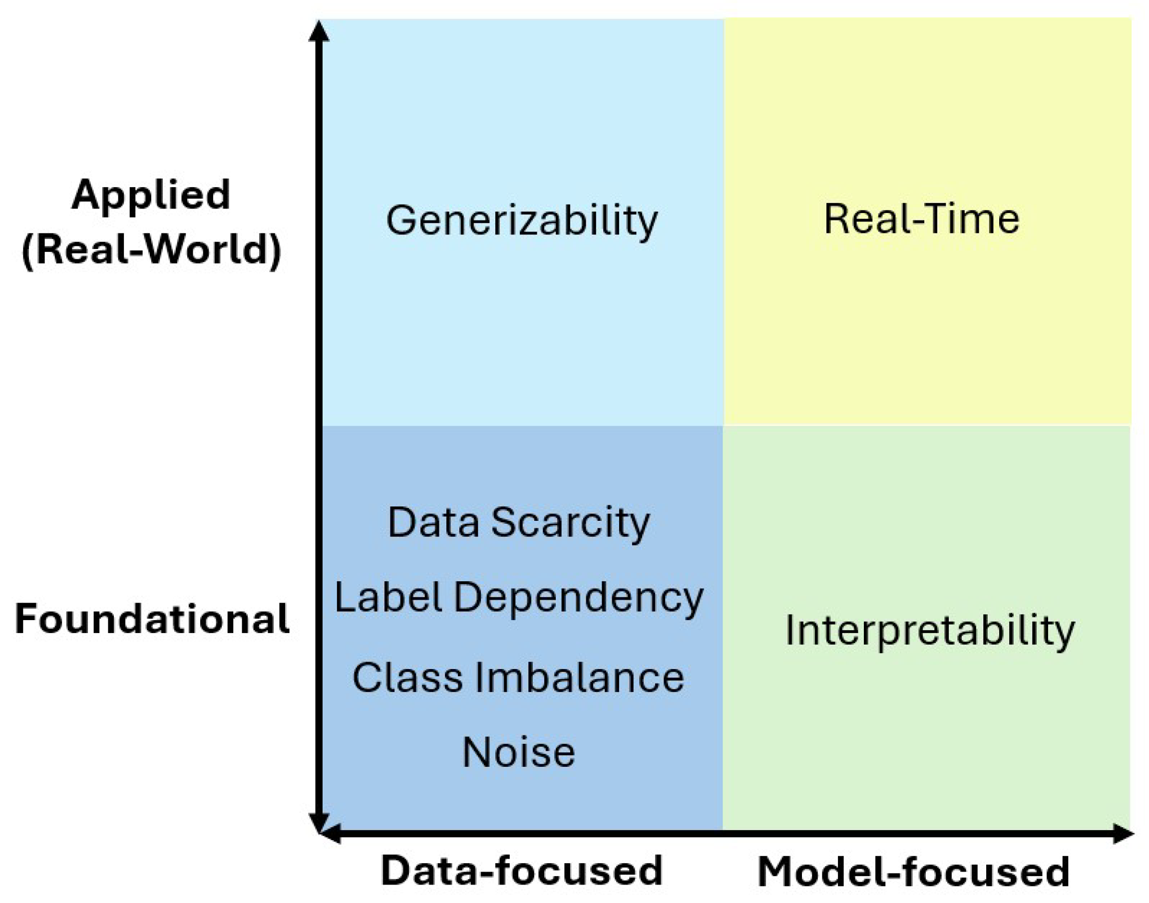
Despite advances in ML and DL for cavitation detection, some key challenges impede reliable deployment. This subsection synthesizes these barriers from reviewed studies, categorizable by the matrix in Figure 9 to reveal their interconnections. It can be seen that foundational data issues must precede applied model solutions for operational success. The challenges are discussed in detail below.

3.6.1. Data Scarcity

ML models demand large datasets for robust training, but cavitation monitoring suffers from limited raw data volumes due to rare events, high acquisition costs and safety constraints. Data scarcity manifests as insufficient signal samples. For instance, Kang et al. tested 5–25% training sizes without augmentation, revealing sharp performance drops for smaller training sizes. This issue can be addressed via simple window overlaps (e.g., [56]) or more complex augmentation techniques like GANs (AC-GANs boosted CNN accuracy from 94.2% to 98.1% [33]; GAN-STFT-Swin Transformer reached 98.6% [37]), geometric transforms (rotation/shift/flip) [11,16], amplitude iteration (129–4030 samples [13]) and physics-informed methods (CFD-CNN-XGBoost hybrid hit 98.95% [8]; use of CFD training dataset [27]).

This differs from label scarcity, where ample unlabeled signals exist but expert annotation is scarce due to subjectivity and intermittency.

3.6.2. Label Dependency

The majority of existing approaches (>83% of the reviewed studies) rely on fully supervised learning, which presupposes the availability of accurate ground-truth labels. However, acquiring such labels under real-world operating conditions is inherently challenging due to the rarity of cavitation events, the subjectivity of expert annotations and associated safety constraints. Consequently, a critical gap remains between laboratory-based model development and the ultimate objective of reliable deployment in real operational environments. To address this limitation, several recent contributions explore strategies to mitigate label dependency through unsupervised, semi-supervised and transfer-based learning approaches.

Unsupervised approaches are primarily applied for anomaly detection. For instance, Cruz Rangel et al. [41] and Siano et al. [28] use unsupervised frameworks to distinguish normal from cavitating conditions. However, purely unsupervised anomaly detection typically yields only a binary separation between normal and abnormal states, without providing detailed information on cavitation intensity or underlying physical phenomena. Favrel et al. [42] extend this concept by combining unsupervised expert-based clustering with supervised ML classification to identify multiple cavitation surge regimes and predict their onset using prototype monitoring data.

As further approaches to address limited label availability, semi-supervised and transfer-based approaches have been proposed. Abrasaldo et al. [14,15] introduce a semi-supervised self-training approach that automatically labels 88% of previously unlabeled data and identifies 20 validated abnormal events, substantially reducing manual annotation effort. Sun et al. [45] leverage predicted distributions from a cavitation state classifier as pseudo-labels for the unlabeled target domain in deep domain adaptation, achieving >93% multi-class cavitation recognition accuracy across varying pump conditions with zero target–domain ground-truth labels. Wang et al. [7] demonstrate that transfer learning can substantially decrease manual annotation efforts.

While promising, these label-efficient methods remain preliminary, with unsupervised approaches limited to binary outcomes and semi-/transfer strategies needing validation at scale.

3.6.3. Class Imbalance

Class imbalance occurs when one class (e.g., normal operation) vastly outnumbers others (e.g., rare severe cavitation), skewing models to favor majority-class predictions at the expense of minorities. In particular, cavitation field datasets exemplify this, with normal states dominating. While proactive studies counter it—Gaisser et al. [11] via balanced accuracy, He et al. [37] with GAN augmentation, Abrasaldo et al. [14,15] through under-sampling—many overlook evident imbalances, undermining severe-event detection. Routine handling via these or hybrid techniques is thus recommended.

3.6.4. Noise

Noise from mechanical vibrations, operator activity and environmental influences can corrupt cavitation signals, obscure diagnostic features and degrade ML performance. Recent studies address this issue through progressively more advanced mitigation strategies:

• Sensor selection and data acquisition (early-stage mitigation): Nasiri et al. [54] apply anti-aliasing low-pass filters to prevent spectral distortion. Karagiovanidi et al. [51] trim the first and last seconds of recorded signals helps remove operator-induced artifacts and Look et al. [33] use ultrasonic sensors to reduce sensitivity to low-frequency mechanical noise.
• Filtering and signal decomposition (interference suppression): Gaisser et al. [11] and Powar et al. [35] use bandpass filtering. He et al. [37] prefer re-emphasis FIR high-pass filters to enhance high-frequency components. Further approaches include FFT-based filtering [13], EMD [7,55] and VMD for suppressing interference signals [25,27,36,57]. Gruber et al. [9] apply outlier rejection strategies.
• Data-driven denoising (learning-based approaches): Implicit denoising is achieved using specific models. Kang et al. [34] and Song et al. [58] use sparse and denoising autoencoders, respectively. Additional techniques include SVD- and wavelet-based denoising [35,43], time–amplitude–time–frequency (TATF) methods [8] and DPCA-based demodulation [16].
• Robustness evaluation (realistic disturbance simulation): Amini et al. [38] assess model robustness by injecting artificial background noise (e.g., jackhammer or crane signals). Dong et al. [5] add white noise to signals.

Overall, the literature demonstrates that effective noise mitigation requires a combination of careful sensor selection, targeted signal processing, data-driven denoising and systematic robustness evaluation to ensure reliable cavitation detection under real operating conditions.

3.6.5. Generalizability

Most studies evaluate cavitation detection models on single machines under controlled laboratory conditions, which limits their applicability in real-world scenarios. Differences in machine-specific acoustics, geometry and scaling, combined with uncontrolled environmental noise, variable loads and wear present in field operations, necessitate robust cross-domain generalization for reliable deployment.

Operating regime generalizability addresses performance across load/speed/flow regimes in one machine via multi-operating regime validation. For example, Wu et al. [24] already spanned 3 flow rates × 10 NPSH values to map cavitation progression and Hasanpour et al. [40] compiled 297 points across seven pumps. This prevents overfitting to narrow regimes and enables reliable monitoring under real-world fluctuations.

Machine-type generalizability addresses machine variability through diverse validation strategies. For example, Hasanpour et al. [40] employ separate SVMs per machine, while their DL approach uses a single combined model across machines. Look et al. [33] implement cross-turbine testing, using dropout, max-pooling and an auxiliary classifier GAN (AC-GAN) with I-divergence to increase synthetic spectrogram diversity, thereby enhancing sensor and turbine robustness. Dong et al. [5] apply multi-point sensor fusion to aggregate complementary perspectives. Abrasaldo et al. [14,15] perform exhaustive leave-one-group-out cross-validation (945 folds) to emulate performance on unseen machines.

Environment and operating-condition generalizability addresses shifts from laboratory to field conditions through transfer learning and domain alignment. Sun et al. [45] employ a multi-adversarial attention network (MAAN), achieving over 93% multi-class accuracy across 12 cross-condition tasks via joint and conditional distribution alignment with predicted pseudo-labels. Wang et al. [7] use CORAL for domain adaptation, while Gaisser et al. [11] combine domain-adversarial training with advanced preprocessing and uncertainty quantification to reduce false alarms. Hajnayeb et al. [56] transfer ImageNet-pretrained CNNs to bispectrum images for error-free detection and Wu et al. [24] demonstrate transfer learning across multiple flow rates.

In summary, robust generalizability in cavitation detection requires addressing both machine-specific variability and changes in environmental or operating conditions. So far this can be achieved through careful validation, sensor fusion and domain-adaptive learning to ensure reliable performance in real-world applications.

3.6.6. Real-Time Capability

Real-time cavitation monitoring is critical for timely detection and control, but it is challenged by high-frequency signals and the computational demands of ML models. Early approaches already focused on computationally efficient architectures: Steele et al. [29] demonstrated viable on-line monitoring with shallow ANNs on raw sensors, Lavretsky [30] achieved online detection using a parallel ordered network on DSPACE, Hocevar [53] demonstrated low-cost adaptive control and Stephen et al. [12] showed that DTs are suitable for real-time use, whereas ANNs are less feasible.

Many studies further optimize performance through dimensionality reduction and feature selection. Dong et al. [5] and Zhang et al. [46] apply PCA, Stephen et al. [12] select the top 18 features via ANOVA and DTs, Azizi [55] reduces computation by selecting fewer IMFs and features, Song et al. [58] remove redundant features and apply automatic hyperparameter optimization and Tong et al. [4] use a two-stage ANN to reduce training time. Several works also evaluate models in terms of both accuracy and computation time [25,45,49], while Kang et al. [31] discuss the impact of network depth on runtime.

Other studies combine fast data acquisition with lightweight processing. Adeodu [63] used IIoT-based sound monitoring with Arduino, Powar [35] transmitted accelerometer data wirelessly to a server for ML-based classification and CruzRangel [41], Durdu [60], Dutta [39], Yu [27] and Tong [4] report real-time capable frameworks, with Tong achieving diagnosis 22–50 times faster than the real-time requirement. Hu [49] achieved 17 ms latency and Siano [28] confirms real-time use with shorter signals.

Overall, these studies show that real-time cavitation detection is feasible through a combination of efficient model architectures, feature reduction, fast data acquisition and edge- or server-based processing, enabling accurate and timely decision-making under operational conditions.

3.6.7. Interpretability

Reliable cavitation monitoring requires models that are not only accurate but also understandable. Without interpretability, operators cannot judge whether an alarm reflects a real issue or sensor artifacts. This makes explainability central in ML/DL-based condition monitoring, particularly in industrial applications where decisions affect safety, availability and maintenance costs. In the literature, several strategies have been proposed to enhance interpretability in ML/DL-based cavitation monitoring, including:

• Applying feature selection: Feature selection like mRMR (minimum redundancy maximum relevance) [34] picks the most useful signal traits while cutting repeats. For classical models like SVMs, simple features—e.g., energy or standard deviation [40]—link predictions to physical signals. Component selection in decomposition pipelines keeps inputs interpretable and physics-grounded [24,55,58]. Feature-importance rankings and sensitivity analysis tie predictions to physical variables [14,15,35], explaining what drives diagnosis and ensuring physical meaning.
• Using inherently interpretable models: DTs [9,12] and neuro-fuzzy systems [60] offer transparent rules. Fu el al. [32] propose interpretable linear fusion of health indices (e.g., RMS and kurtosis) with positive/negative weights justified theoretically (positive for increasing HIs, negative for decreasing), applied to turbine cavitation acoustics for status identification.
• Visualizing model and data structures: Clustering and low-dimensional embeddings reveal separability between operating regimes [38], while parameter-space visualizations relate decision boundaries to operating conditions [42]. Grad-CAM and t-SNE highlight which time–frequency regions or features drive predictions [6,25]. These tools help indicate model focus, but highlighted regions are not automatically causal and may shift with preprocessing or dataset composition.
• Integrating uncertainty into explanations: Ensembles producing predictive probabilities and uncertainty allow operators to handle ambiguous cases safely, such as near incipient cavitation [11]. This supports staged alarms, requests for additional evidence and safer operational decisions when model predictions are uncertain.

Taken together, interpretability in cavitation and efficiency monitoring is best achieved by combining physically meaningful inputs, transparent model behavior or faithful post hoc explanations, quantified uncertainty and validation across operating conditions. Physics-informed approaches, reinforce this chain by constraining learning in ways that are both credible and physically justifiable.

4. Discussion

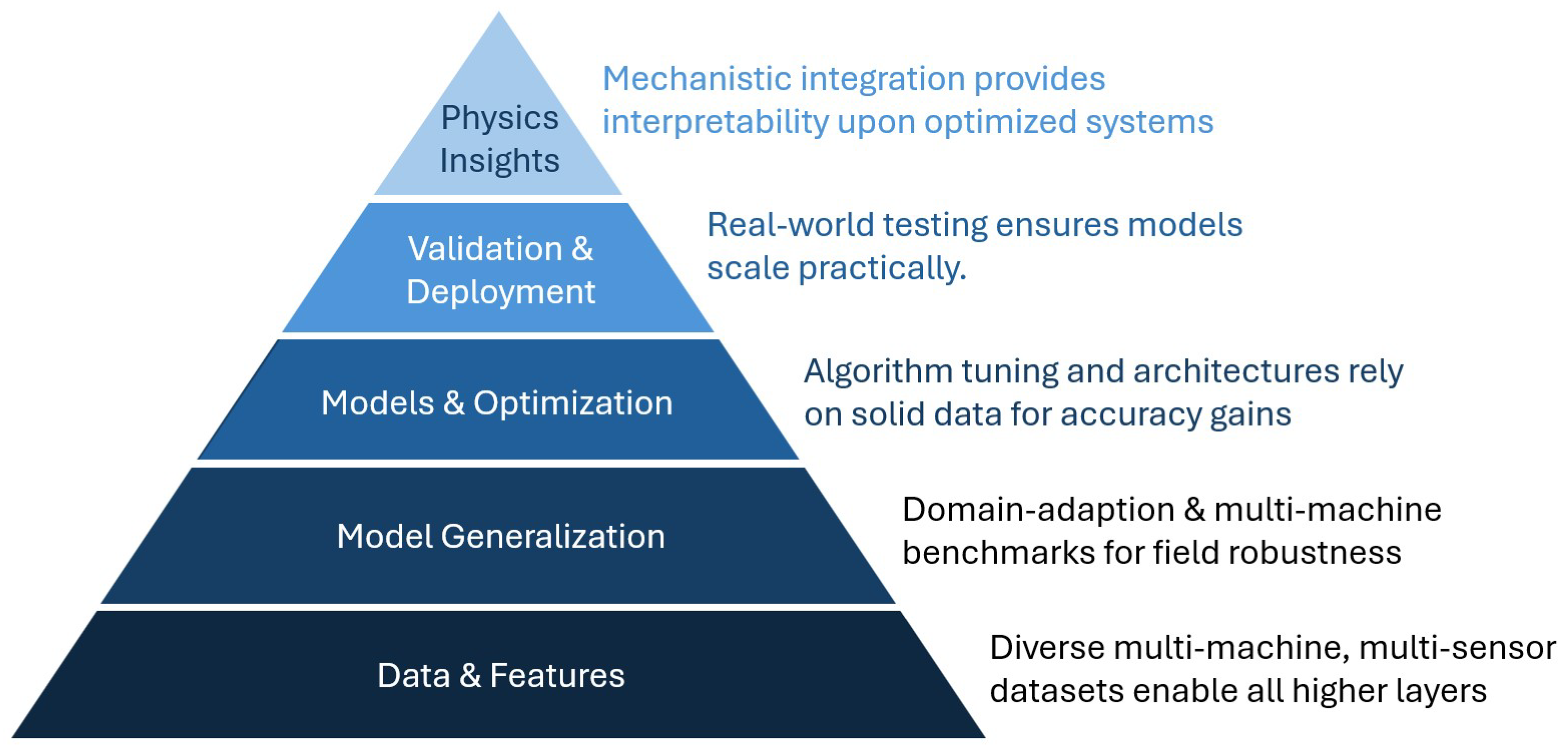
This scoping review of 52 studies on ML/DL for cavitation monitoring—from machinery characteristics and data acquisition to data preparation, modeling and deployment—reveals a maturing field with evolutionary patterns, biases and priorities. The following synthesizes key insights addressing the research questions.

RQ1—Machinery and contexts: Studies predominantly focus on pumps (71% of works), especially centrifugal pumps (50%), while turbines represent only 23% (mainly Francis units) and specialized variants like axial piston pumps remain rare. Over 80% of the studies rely on single-machine datasets and laboratory test rigs for controlled regimes and high-fidelity labeling (e.g., visual/NPSH-based), limiting cross-machine transferability and amplifying lab-to-field domain shifts. Field studies (scarce at <20%) often lack generalizability testing, underscoring the need for hybrid lab-field validation.

RQ2—Sensing and data acquisition: Vibration dominates for pumps, acoustics for turbines, with hybrids outperforming single modalities by capturing complementary physics. Low-cost/non-intrusive options (motor current, IoT MEMS, smartphones) are gaining traction for field scalability, though benefits accrue from strategic placement near cavitation sources rather than sheer sensor count. The analyzed operating regimes are mostly steady-state, labeled via visuals (lab), NPSH/head-drop or experts (field)—creating label scarcity/noise, especially for transients.

RQ3—Data preparation: Raw time–domain feeds end-to-end DL, but most studies transform to frequency (FFT) or time–frequency (STFT/CWT) domains to reveal cavitation broadband noise/sidebands, with adaptive decompositions (VMD/EMD) isolating informative modes. Feature extraction evolves from physics-guided manual stats (RMS, kurtosis, peaks; interpretable/low-data) to automatic DL learning (CNNs on spectrograms) and hybrids, balancing performance/interpretability. Signal representations as input to the ML models range from 1D numerical vectors (classical ML) to 2D images (DL), with no universal optimum—context-dependent on data size and goals.

RQ4—Monitoring objectives and model architectures: Objectives progress from binary detection (simple alarms) to multiclass severity (3–4 levels dominant; up to 10 states), prediction of specific cavitation indication values and hybrids—trading simplicity for richer diagnostics. Classical ML persists alongside shallow NNs, but DL leads recent advances. Hybrids (DL features + classical classifiers, or handcrafted features + DL) blend strong performance with interpretability. Ultimately, no single architecture reigns supreme; optimal selection depends on balancing data availability, computational constraints and explanability requirements. Severity classification remains the dominant objective (e.g., none/mild/severe based on NPSH or similar indicators). However, no reviewed work focuses on the complex, nonlinear relationship between cavitation intensity and material damage (erosion). Future research must bridge this gap by developing ML methods for cavitation monitoring in combination with erosion prediction and remaining useful life (RUL) estimation.

RQ5—Performance and efficacy: Reported performance strongly depends on the underlying assumptions, data quality and experimental setup. Across the reviewed studies, classical ML approaches typically achieve accuracies in the range of 94.2–99%, often benefiting from higher interpretability and lower data requirements. Shallow neural networks show a wider performance spread (81–100%), while deep learning models reach reported accuracies between 87.2 and 100%, frequently performing best on more complex tasks. Hybrid approaches aim to combine these advantages, e.g., ML models enhanced with DL-level performance or DL models improved in terms of interpretability. Overall, reported performance has increased over time, with more recent methods often achieving higher gains. Laboratory studies routinely report 94–100% accuracy (range 81–100%) for binary classification and comparable 95–99% (range 87.2–99.9%) for multi-class severity classification. Quantification via regression proves reliable where applied but remains sparse across studies, currently limiting precise cavitation intensity and efficiency loss assessment. Field/semi-supervised deployment and multi-prototype generalization reduce results (e.g., only 70% mean validation accuracy for a validation with 5 prototypes), revealing key reliability gaps for practical monitoring. While most studies rely on labeled data from laboratory measurements, expert interpretation or operational indicators, the extent to which ML/DL predictions generalize beyond these controlled labels remains unclear. Systematic comparisons with theoretical or numerical predictions remain absent, leaving the confidence and trustworthiness of AI-based predictions under real operational conditions insufficiently quantified. Addressing this gap through standardized validation protocols, cross-condition benchmarking and multi-prototype studies is essential to enable reliable and deployable ML/DL diagnostics in hydraulic machinery.

RQ6—Challenges and gaps: Data scarcity, domain shifts across conditions and sensors, noisy labels and class imbalance persistently challenge ML/DL applications, driving innovations such as GAN-based augmentation, domain adaptation and physics-informed designs. Deployment demands edge-ready robustness, while transients remain underexplored. Crucially, while most studies rely on labeled datasets, the confidence and trustworthiness of ML/DL predictions across machines, operating conditions and field scenarios remains largely unquantified. Key priorities include multi-machine field datasets, semi-supervised analysis, explainable hybrids and standardized cross-condition validation protocols to enable scalable, reliable and trustworthy diagnostics.

While ML and DL show strong potential for cavitation monitoring—particularly in capturing nonlinearities and uncovering complex patterns—they must be applied thoughtfully and in the right context. Although high accuracies are often reported under controlled conditions, their real-world reliability depends on data quality, representativeness and robustness to domain shifts. Rather than serving as a direct substitute for established physical models, ML/DL open up new possibilities for enhanced diagnostics, early detection and data-driven insights. Their greatest value lies in complementing and extending traditional approaches, combining the strengths of both data-driven and physics-based methods.

Further Research Directions

While current ML/DL methods show promise for cavitation detection, the studies consistently highlight gaps in robustness, scalability and real-world deployment—necessitating targeted advances to transition from prototypes to operational tools. These directions form a pyramid framework (Figure 10), where data strategies provide the essential foundation enabling model optimization, which supports validation and deployment, culminating in physics insights for full interpretability—each layer building the basis for the success of the next. The most generic and important further research directions can be grouped as follows:

• Data and Feature Strategies

  -

  Collect larger and more diverse datasets across operating conditions and machine types to enable multi-machine validation [4,12,25,27,45,51].

  -

  Standardize cavitation labels for unified benchmarks, resolving inconsistencies that hinder ML comparisons.

  -

  Integrate multi-sensor data for richer feature representation and improved robustness [8,9,25,27].

• Model Generalization

  -

  Data level: Develop multi-machine, multi-condition benchmark datasets (e.g., lab-to-field, pump-to-turbine) with standardized labeling to enable transferable training and fair comparison.

  -

  Algorithm level: Leverage domain adaptation, transfer learning and meta-learning to improve robustness and enable efficient adaptation to new machines and operating conditions [11,38].

  -

  Evaluation level: Establish standardized cross-machine and cross-condition validation protocols to reliably assess generalization performance beyond single setups.

• Model and Algorithm Optimization

  -

  Optimize classifiers and hyperparameters [42,50,51].

  -

  Explore automated ML [38], transfer learning [38] and physics-informed neural networks [27].

  -

  Investigate alternative architectures (CNN alternatives, generative models) for low-SNR efficiency and better generalization [8,15].

  -

  Automate workflows for scalable deployment, including computational efficiency and anti-interference improvements for high-noise scenarios [5,15,42].

• Real-World Validation and Deployment

  -

  Test and validate models under operational conditions; examine generalizability versus site-specific training [9,15,16,25,51].

  -

  Develop real-time monitoring systems, including mobile or edge-device integration for practical field deployment [12,27,49].

  -

  Handle corrupted or incomplete signals [11], dynamic conditions [12] and class-specific weighting for improved reliability [6].

  -

  Quantify prediction confidence via multi-prototype and cross-condition benchmarking to ensure AI reliability in real-world operation.

• Physics and Mechanistic Insights

  -

  Better understand cavitation phenomena, including types [29,33,53], blade losses [13] and operational mechanisms [53].

  -

  Characterize cavitation types via their sensor signatures to guide feature selection and enable type-specific ML detection.

  -

  Refine detection for specific fault types and operational scenarios [28].

  -

  Integrate physics-informed modeling approaches to enhance interpretability and guide ML feature selection [27].

  -

  Develop ML models linking cavitation intensity to erosion prediction and RUL estimation, addressing the complex nonlinear damage relationship.

Addressing these directions will be essential to advance ML/DL approaches from controlled studies to robust, scalable and interpretable tools capable of reliable cavitation monitoring in real-world operation.

5. Conclusions

This scoping review highlights that ML and DL for cavitation monitoring is a rapidly evolving yet still maturing field. Research has concentrated largely on pumps under controlled laboratory conditions, with turbines and field-scale studies remaining underrepresented. Sensor modalities, data preparation strategies and modeling approaches are diversifying, with hybrid and physics-informed methods increasingly bridging the gap between performance and interpretability. Importantly, unlike traditional threshold- or spectral-based methods (with their limitations), ML/DL uniquely captures nonlinear interactions for early cavitation detection—offering adaptive, predictive diagnostics in complex regimes. Despite high accuracies in controlled setups, challenges such as data scarcity, domain shifts, noisy labels, transient regimes and the lack of cross-machine validation limit real-world deployment. Moreover, the nonlinear link between cavitation intensity and material damage remains largely unaddressed, leaving erosion prediction and remaining useful life (RUL) estimation as key open problems.

Building on the pyramid framework (Figure 10), future work should target the following areas:

• Data and Feature Strategies: Expand multi-machine, multi-condition datasets with standardized labels and integrate complementary sensor modalities for richer feature representations.
• Model Generalization: Develop domain-adaptive, transfer learning and meta-learning approaches; implement standardized cross-machine and cross-condition evaluation protocols to ensure robust generalization.
• Model and Algorithm Optimization: Explore hybrid and physics-informed architectures, automated ML workflows and architectures resilient to low-SNR, transient and noisy data.
• Real-World Validation and Deployment: Conduct field validation under operational conditions, integrate edge-ready monitoring systems and handle incomplete or corrupted signals to ensure practical reliability.
• Physics and Mechanistic Insights: Link ML predictions to cavitation intensity, erosion risk and RUL; integrate physics-informed multi-sensor fusion to improve interpretability and support predictive maintenance.

Together, these priorities provide a structured roadmap to advance ML/DL approaches from controlled experiments toward robust, deployable and interpretable tools, enabling earlier detection, reliable diagnostics and improved operational safety and efficiency in hydraulic machinery.

References

1. Avellan, F. Introduction to cavitation in hydraulic machinery. In Proceedings of the 6th International Conference on Hydraulic Machinery and Hydrodynamics, Perth, WA, Australia, 24–26 November 2004; pp. 11–22. [Google Scholar]
2. Kumar, P.; Saini, R. Study of cavitation in hydro turbines—A review. Renew. Sustain. Energy Rev. 2010, 14, 374–383. [Google Scholar] [CrossRef] [Scilit]
3. Binama, M.; Muhirwa, A.; Bisengimana, E. Cavitation Effects in Centrifugal Pumps—A Review. Int. J. Eng. Res. Appl. (IJERA) 2016, 6, 52–63. [Google Scholar]
4. Tong, Z.; Liu, H.; Cao, X.E.; Westerdahld, D.; Jin, X. Cavitation diagnosis for water distribution pumps: An early-stage approach combing vibration signal-based neural network with high-speed photography. Sustain. Energy Technol. Assess. 2023, 55, 102919. [Google Scholar] [CrossRef] [Scilit]
5. Dong, L.; Zhu, J.; Wu, K.; Dai, C.; Liu, H.; Zhang, L.; Guo, J.; Lin, H. Cavitation Status Recognition Method of Centrifugal Pump Based on Multi-Pointand Multi-Resolution Analysis. J. Appl. Fluid Mech. 2021, 14, 315–329. [Google Scholar] [CrossRef] [Scilit]
6. Chao, Q.; Wei, X.; Tao, J.; Liu, C.; Wang, Y. Cavitation recognition of axial piston pumps in noisy environment based on Grad-CAM visualization technique. CAAI Trans. Intell. Technol. 2023, 8, 206–218. [Google Scholar] [CrossRef] [Scilit]
7. Wang, R.; Xu, Y.; Mu, W.; Chen, Y.; Jiao, Z. Cavitation intensity recognition for axial piston pump based on transient flow rate measurement and improved transfer learning method. Mech. Syst. Signal Process. 2025, 232, 112667. [Google Scholar] [CrossRef] [Scilit]
8. Yin, F.; Ma, Z.; Zhang, Y.; Ma, Z.; Nie, S.; Ji, H. Cavitation detection for water hydraulic axial piston pump based on physics-informed CNN data augmentation and XGBoost. Mech. Syst. Signal Process. 2025, 241, 113512. [Google Scholar] [CrossRef] [Scilit]
9. Gruber, P.; Farhat, M.; Odermatt, P.; Etterlin, M.; Lerch, T.; Frei, M. The detection of cavitation in hydraulic machines by use of ultrasonic signal analysis. Int. J. Fluid Mach. Syst. 2015, 8, 264–273. [Google Scholar] [CrossRef] [Scilit]
10. Escaler, X.; Egusquiza, E.; Farhat, M.; Avellan, F.; Coussirat, M. Detection of cavitation in hydraulic turbines. Mech. Syst. Signal Process. 2006, 20, 983–1007. [Google Scholar] [CrossRef] [Scilit]
11. Gaisser, L.; Kirschner, O.; Riedelbauch, S. Cavitation detection in hydraulic machinery by analyzing acoustic emissions under strong domain shifts using neural networks. Phys. Fluids 2023, 35, 027128. [Google Scholar] [CrossRef] [Scilit]
12. Stephen, C.; Basu, B.; McNabola, A. Evaluation of supervised machine learning techniques for cavitation detection and diagnosis in a pump-as-turbine system. Expert Syst. Appl. 2026, 296, 129167. [Google Scholar] [CrossRef] [Scilit]
13. de Souza, J.C.S.; Júnior, O.H.; Filho, G.L.T.; Carpinteiro, O.A.S.; Biancardine Júnior, H.S.D.; Dos Santos, I.F.S. Application of machine learning models in predictive maintenance of Francis hydraulic turbines. Rev. Bras. Recur. Hidr. 2024, 3–14. [Google Scholar] [CrossRef] [Scilit]
14. Abrasaldo, P.M.B.; Zarrouk, S.J.; Kempa-Liehr, A.W.; Mudie, A.; Cen, J.; Siega, C. Detecting Abnormal Events in Geothermal Power Plant Time-Series Data Using a Semi-Supervised Machine Learning Approach. Trans.-Geotherm. Resour. Counc. 2023, 47, 2281–2298. [Google Scholar]
15. Michael B. Abrasaldo, P.; Zarrouk, S.J.; Mudie, A.; Cen, J.; Siega, C.; Kempa-Liehr, A.W. Detection of abnormal operation in geothermal binary plant feed pumps using time-series analytics. Expert Syst. Appl. 2024, 247, 123305. [Google Scholar] [CrossRef] [Scilit]
16. Song, Y.; Zhang, T.; Liu, Q.; Ge, B.; Liu, J.; Zhang, L. Cavitation Identification Method of Centrifugal Pumps Based on Signal Demodulation and EfficientNet. Arab. J. Sci. Eng. 2025, 50, 8779–8793. [Google Scholar] [CrossRef] [Scilit]
17. Luo, X.W.; Ji, B.; Tsujimoto, Y. A review of cavitation in hydraulic machinery. J. Hydrodyn. Ser. B 2016, 28, 335–358. [Google Scholar] [CrossRef] [Scilit]
18. Lei, Y.; Yang, B.; Jiang, X.; Jia, F.; Li, N.; Nandi, A.K. Applications of machine learning to machine fault diagnosis: A review and roadmap. Mech. Syst. Signal Process. 2020, 138, 106587. [Google Scholar] [CrossRef] [Scilit]
19. Matania, O.; Dattner, I.; Bortman, J.; Kenett, R.S.; Parmet, Y. A systematic literature review of deep learning for vibration-based fault diagnosis of critical rotating machinery: Limitations and challenges. J. Sound Vib. 2024, 590, 118562. [Google Scholar] [CrossRef] [Scilit]
20. Sha, Y.; Liu, N.; Liu, H.; Tao, J.; Niu, Z.; Huang, G.; Yao, Y.; Liang, J.; Qian, M.; Stoecker, H.; et al. A Review of Machine Learning for Cavitation Intensity Recognition in Complex Industrial Systems. arXiv 2025, arXiv:2511.15497. [Google Scholar] [CrossRef] [Scilit]
21. Tricco, A.C.; Lillie, E.; Zarin, W.; O’Brien, K.K.; Colquhoun, H.; Levac, D.; Moher, D.; Peters, M.D.J.; Horsley, T.; Weeks, L.; et al. PRISMA Extension for Scoping Reviews (PRISMA-ScR): Checklist and Explanation. Ann. Intern. Med. 2018, 169, 467–473. [Google Scholar] [CrossRef] [Scilit] [PubMed]
22. Peters, M.D.J.; Godfrey, C.; McInerney, P.; Munn, Z.; Tricco, A.C.; Khalil, H. Scoping Reviews. In JBI Manual for Evidence Synthesis; Aromataris, E., Lockwood, C., Porritt, K., Pilla, B., Jordan, Z., Eds.; JBI: Adelaide, Australia, 2024. [Google Scholar] [CrossRef] [Scilit]
23. Page, M.J.; McKenzie, J.E.; Bossuyt, P.M.; Boutron, I.; Hoffmann, T.C.; Mulrow, C.D.; Shamseer, L.; Tetzlaff, J.M.; Akl, E.A.; Brennan, S.E.; et al. The PRISMA 2020 statement: An updated guideline for reporting systematic reviews. BMJ 2021, 372, n71. [Google Scholar] [CrossRef] [Scilit] [PubMed]
24. Wu, K.; Xing, Y.; Chu, N.; Wu, P.; Cao, L.; Wu, D. A carrier wave extraction method for cavitation characterization based on time synchronous average and time-frequency analysis. J. Sound Vib. 2020, 489, 115682. [Google Scholar] [CrossRef] [Scilit]
25. Li, X.; Wu, G.; Wu, P. VMD-SE-DCNN-CBAM: An Intelligent Cavitation Recognition Method for Canned Motor Pump. IEEE Trans. Instrum. Meas. 2025, 74, 1–13. [Google Scholar] [CrossRef] [Scilit]
26. Tan, Y.; Wu, G.; Qiu, Y.; Fan, H.; Wan, J. Fault diagnosis of a mixed-flow pump under cavitation condition based on deep learning techniques. Front. Energy Res. 2023, 10, 1109214. [Google Scholar] [CrossRef] [Scilit]
27. Yu, L.; Cheng, L. Cavitation Coefficient Identification Model for an Axial Flow Pump Based on Pressure Signal Feature Extraction and Spider Wasp Optimization Algorithm. J. Mar. Sci. Eng. 2026, 14, 18. [Google Scholar] [CrossRef] [Scilit]
28. Siano, D.; Panza, M. Diagnostic method by using vibration analysis for pump fault detection. Energy Procedia 2018, 148, 10–17. [Google Scholar] [CrossRef] [Scilit]
29. Steele, J.P.H.; Archuleta, M.; Hooley, T. Detecting cavitation in hydraulic pumps using artificial neural networks. Intell. Eng. Syst. Through Artif. Neural Netw. 1996, 6, 909–914. [Google Scholar]
30. Lavretsky, E.; Chidambaram, B. Health monitoring of an electro-hydraulic system using ordered neural networks. In Proceedings of the 2002 International Joint Conference on Neural Networks, Honolulu, HI, USA, 12–17 May 2002; IJCNN’02 (Cat. No. 02CH37290); IEEE: Piscataway, NJ, USA, 2002; Volume 3, pp. 2893–2898. [Google Scholar] [CrossRef] [Scilit]
31. Kang, Z.; Liu, Z. Analysis of Optimal Parameters for Discriminating Cavitation Types by SSAE-RF. J. Phys. Conf. Ser. 2022, 2242, 012025. [Google Scholar] [CrossRef] [Scilit]
32. Fu, Y.; Chen, Y.; Wang, D.; Peng, Z. Interpretable fusion methodology of health indices with an application to industrial turbine cavitation condition monitoring. Philos. Trans. R. Soc. A Math. Phys. Eng. Sci. 2024, 382, 20220402. [Google Scholar] [CrossRef] [Scilit] [PubMed]
33. Look, A.; Kirschner, O.; Riedelbauch, S. Building robust classifiers with generative adversarial networks for detecting cavitation in hydraulic turbines. In Proceedings of the ICPRAM 2018—the 7th International Conference on Pattern Recognition Applications and Methods, Madeira, Portugal, 16–18 January 2018; pp. 456–462. [Google Scholar] [CrossRef] [Scilit]
34. Kang, Z.; Feng, C.; Wan, X.; Liu, Z.; Chen, L. Stacked sparse autoencoder in cavitation noise signal data classification of hydro turbine based on power spectrum. J. Low Freq. Noise Vib. Act. Control 2020, 39, 233–245. [Google Scholar] [CrossRef] [Scilit]
35. Powar, S.K.; Cohen, S.; Ratnaparkhi, S.; Satpute, N. Vortex to Cavitation: Enhancing Turbine Safety and Efficiency. In Proceedings of the 2025 International Conference on Applications of Machine Intelligence and Data Analytics (ICAMIDA), Aurangabad, India, 21–22 August 2025; pp. 1–6. [Google Scholar] [CrossRef] [Scilit]
36. Zhao, Y.; Yan, S.; Li, Z.; Chen, F.; Zhao, Q.; He, L.; Wu, H.; Bai, Y.; Yang, X. Optimizing cavitation fault forecasting in pump-turbine systems through gated recurrent units. Phys. Fluids 2025, 37, 037124. [Google Scholar] [CrossRef] [Scilit]
37. He, J.; Hao, J.; Cao, Z. SGST: A Novel Approach Based on Machine Learning for Cavitation Fault Diagnosis. In Proceedings of the IECON 2023—The 49th Annual Conference of the IEEE Industrial Electronics Society, Singapore, 16–19 October 2023; pp. 1–7. [Google Scholar] [CrossRef] [Scilit]
38. Amini, A.; Pacot, O.; Voide, D.; Hasmatuchi, V.; Roduit, P.; Munch-Alligne, C. Development of a Novel Cavitation Monitoring System for Hydro Turbines Based on Machine Learning Algorithms. IOP Conf. Ser. Earth Environ. Sci. 2022, 1079, 012015. [Google Scholar] [CrossRef] [Scilit]
39. Dutta, N.; Subramaniam, U.; Sanjeevikumar, P.; Bharadwaj, S.C.; Leonowicz, Z.; Holm-Nielsen, J.B. Comparative Study of Cavitation Problem Detection in Pumping System Using SVM and K-Nearest Neighbour Method. In Proceedings of the 2020 IEEE International Conference on Environment and Electrical Engineering and 2020 IEEE Industrial and Commercial Power Systems Europe (EEEIC/I&CPS Europe), Madrid, Spain, 9–12 June 2020; pp. 1–6. [Google Scholar] [CrossRef] [Scilit]
40. Hasanpour, M.A.; Engholm, R.; Fafoutis, X. Pump Cavitation Detection with Machine Learning: A Comparative Study of SVM and Deep Learning. In Proceedings of the 2024 IEEE Annual Congress on Artificial Intelligence of Things (AIoT), Melbourne, Australia, 24–26 July 2024; pp. 219–225. [Google Scholar] [CrossRef] [Scilit]
41. Cruz-Rangel, D.; Perurena-Landache, N.; De-La-Fuente-Azpeitia, N.; Ocampo-Martinez, C.; Diaz-Rozo, J. Online Current Signature Analysis Approach for Cavitation Assessment in Hydraulic Pumps. IFAC-PapersOnLine 2025, 59, 49–54. [Google Scholar] [CrossRef] [Scilit]
42. Favrel, A.; Kahwati, G.; Dollon, Q. Identification of full-load cavitation surge onset in hydropower units through the clustering of monitoring data. IOP Conf. Ser. Earth Environ. Sci. 2025, 1483, 012005. [Google Scholar] [CrossRef] [Scilit]
43. Song, M.; Zhi, Y.; An, M.; Xu, W.; Li, G.; Wang, X. Centrifugal Pump Cavitation Fault Diagnosis Based on Feature-Level Multi-Source Information Fusion. Processes 2024, 12, 196. [Google Scholar] [CrossRef] [Scilit]
44. Dong, L.; Wu, K.; Zhu, J.C.; Dai, C.; Zhang, L.X.; Guo, J.N. Cavitation Detection in Centrifugal Pump Based on Interior Flow-Borne Noise Using WPD-PCA-RBF. Shock Vib. 2019, 2019, 8768043. [Google Scholar] [CrossRef] [Scilit]
45. Sun, B.; Zhang, Z.; Dong, P.; Zeng, Y.; Wang, L.; Yang, S.; Wu, K.; Wu, D. Cavitation state recognition of centrifugal pumps across various working conditions by Multi-Adversarial Attention Network. Mech. Syst. Signal Process. 2025, 239, 113336. [Google Scholar] [CrossRef] [Scilit]
46. Zhang, T.; Song, Y.; Liu, Q.; Ge, Y.; Zhang, L.; Liu, J. Cavitation state recognition method of centrifugal pump based on multi-dimensional feature fusion and convolutional gate recurrent unit. Phys. Fluids 2024, 36, 105149. [Google Scholar] [CrossRef] [Scilit]
47. Stephen, C.; Guguloth, V.; Sivasailam, K.; Gu, Y.; Parmar, R.; Banerjee, C. Prediction of cavitation using machine learning techniques on centrifugal pump. J. Phys. Conf. Ser. 2024, 2854, 012014. [Google Scholar] [CrossRef] [Scilit]
48. Won, I.H.; Gao, R.; Tsoukalas, L.H.; Eryurek, E.; Kavaklioglu, K. Incipient cavitation detection methodology using current sensor based on a neural wavelet approach. In Proceedings of the American Nuclear Society—International Congress on Advances in Nuclear Power Plants 2005, ICAPP’05, Seoul, Republic of Korea, 15–19 May 2005; Volume 6, pp. 3243–3249. [Google Scholar]
49. Hu, Q.; Ohata, E.F.; Silva, F.H.; Ramalho, G.L.; Han, T.; Rebouças Filho, P.P. A new online approach for classification of pumps vibration patterns based on intelligent IoT system. Meas. J. Int. Meas. Confed. 2020, 151, 107138. [Google Scholar] [CrossRef] [Scilit]
50. Arendra, A.; Akhmad, S.; Winarso, K.; Herianto. Investigating pump cavitation based on audio sound signature recognition using artificial neural network. J. Phys. Conf. Ser. 2020, 1569, 032044. [Google Scholar] [CrossRef] [Scilit]
51. Karagiovanidis, M.; Pantazi, X.E.; Papamichail, D.; Fragos, V. Early Detection of Cavitation in Centrifugal Pumps Using Low-Cost Vibration and Sound Sensors. Agriculture 2023, 13, 1544. [Google Scholar] [CrossRef] [Scilit]
52. Hajnayeb, A.; Azizi, R.; Ghanbarzadeh, A.; Changizian, M. Vibration-based cavitation detection in centrifugal pumps. Diagnostyka 2017, 18, 77–83. [Google Scholar]
53. Hočevar, M.; Širok, B.; Blagojevič, B. Prediction of cavitation vortex dynamics in the draft tube of a francis turbine using radial basis neural networks. Neural Comput. Appl. 2005, 14, 229–234. [Google Scholar] [CrossRef] [Scilit]
54. Nasiri, M.; Mahjoob, M.; Vahid-Alizadeh, H. Vibration signature analysis for detecting cavitation in centrifugal pumps using neural networks. In Proceedings of the 2011 IEEE International Conference on Mechatronics, Istanbul, Turkey, 13–15 April 2011; pp. 632–635. [Google Scholar] [CrossRef] [Scilit]
55. Azizi, R.; Attaran, B.; Hajnayeb, A.; Ghanbarzadeh, A.; Changizian, M. Improving accuracy of cavitation severity detection in centrifugal pumps using a hybrid feature selection technique. Meas. J. Int. Meas. Confed. 2017, 108, 9–17. [Google Scholar] [CrossRef] [Scilit]
56. Hajnayeb, A. Cavitation Analysis in Centrifugal Pumps Based on Vibration Bispectrum and Transfer Learning. Shock Vib. 2021, 2021, 6988949. [Google Scholar] [CrossRef] [Scilit]
57. Lang, T.; Ni, C.; Chen, K.; Xu, E.; Yin, J.; Shen, X.; Wu, X.; Zhang, D. Recognition of cavitation characteristics in non-clogging pumps based on the improved Lévy flight bat algorithm. Front. Energy Res. 2023, 11, 1335227. [Google Scholar] [CrossRef] [Scilit]
58. Song, H.; Sun, H.; Chen, N. Cavitation fault diagnosis of centrifugal pump based on RIME-SDAE. Vibroeng. Procedia 2024, 54, 46–52. [Google Scholar] [CrossRef] [Scilit]
59. Matloobi, S.M.; Riahi, M. Identification of cavitation in centrifugal pump by artificial immune network. Proc. Inst. Mech. Eng. Part E J. Process Mech. Eng. 2021, 235, 2271–2280. [Google Scholar] [CrossRef] [Scilit]
60. Durdu, A.; Çeltek, S.A.; Orhan, N. Detection of Vortex Cavitation with The Method Adaptive Neural Fuzzy Networks in the Deep Well Pumps. J. Tekirdag Agric. Fac. 2021, 18, 613–624. [Google Scholar] [CrossRef] [Scilit]
61. Nuri, O.; Mehmet, K.; Hasan, K.; Murat, E. Machine Learning-Based Prediction of NPSH, Noise, and Vibration Levels in Radial Pumps Under Cavitation Conditions. J. Tekirdag Agric. Fac. 2024, 21, 533–546. [Google Scholar] [CrossRef] [Scilit]
62. Li, F.; Wang, C.; Liu, Z.; Huang, Y.; Wang, T. Sparrow search algorithm-optimized variational mode decomposition-based multiscale convolutional network for cavitation diagnosis of hydro turbines. Ocean Eng. 2024, 312, 119055. [Google Scholar] [CrossRef] [Scilit]
63. Adeodu, A.; Daniyan, I.; Omitola, O.; Ejimuda, C.; Agbor, E.; Akinola, O. An adaptive Industrial Internet of things (IIOts) based technology for prediction and control of cavitation in centrifugal pumps. Procedia CIRP 2020, 91, 927–934. [Google Scholar] [CrossRef] [Scilit]
Figure 1. PRISMA flowchart: 217 records to 52 included studies.
Applsci 16 03566 g001
Figure 2. ML cavitation monitoring pipeline from machinery to deployment.
Applsci 16 03566 g002
Figure 3. Distribution of machinery types (left), amount of machines analyzed (right top); may include multiple identical units) and monitoring environments (right bottom) across the reviewed studies.
Applsci 16 03566 g003
Figure 4. Exemplary signal representations: time domain (left), frequency domain (middle) and time–frequency distribution (right).
Applsci 16 03566 g004
Figure 5. Evolution of ML publications for cavitation detection (1996–2026), segmented by paradigm: classical ML, shallow ANN, hybrids, DL and combinations.
Applsci 16 03566 g005
Figure 6. General monitoring objectives (left) and severity classification detail ((right): number of classes).
Applsci 16 03566 g006
Figure 7. Hierarchical tree of monitoring objectives with associated study counts.
Applsci 16 03566 g007
Figure 8. Progression of ML architectures for cavitation detection, highlighting advantages and trade-offs.
Applsci 16 03566 g008
Figure 9. Matrix of the identified main challenges: foundational/applied (vertical) × data/model-focused (horizontal).
Applsci 16 03566 g009
Figure 10. Pyramid of future research priorities: data strategies (base) building to physics insights (apex).
Applsci 16 03566 g010