1. Introduction
The aero-engine Secondary Air System (SAS) is a critical subsystem that ensures safe engine operation [
1]. Operating over long durations in an extreme environment characterized by the coupled effects of high temperature, high pressure, and high rotational speed, its internal structures face a substantial risk of sudden failure. Such failures typically occur on a millisecond timescale and are accompanied by abrupt changes in flow-path geometry and boundary conditions, thereby inducing a fast transient response in the SAS. During these events, sudden structural failures can lead to a partial loss of air-system functions, resulting in rapid variations in pressure and mass flow and disrupting normal engine operation; in severe cases, hazardous consequences may arise. Taking shaft fracture as a representative sudden failure scenario, Ref. [
2] reports that a turbine shaft may fracture within approximately 10 ms; once the load is lost, the turbine can rapidly accelerate to its burst speed, generating high-energy fragments and posing a risk of casing penetration. In accordance with airworthiness requirements such as FAR-33 [
3], passive safety design must be implemented to mitigate the accident risk induced by such failures. Therefore, investigating the mechanisms and predictive methods of the fast transient SAS response triggered by sudden structural failures is of significant engineering importance for passive safety design.
As an internal-flow system, the SAS features boundary conditions that are intrinsically coupled to the mainstream flow path and the overall system state; studies of fast transient behavior therefore typically must account for multi-boundary coupling at the engine level [
4]. Owing to the complex flow-path topology, millisecond-scale rapid transients, and strong coupling among multiple engine boundaries, full-engine destructive testing is prohibitively expensive and rarely provides access to internal flow-field details under extreme conditions [
5]. Although three-dimensional CFD can deliver high fidelity, it demands substantial computational resources and remains impractical for long-duration, full-engine-scale dynamic simulations [
6]. Consequently, engineering analyses commonly rely on reduced-order, system-level approaches: the SAS is represented using a network method and is solved in a coupled manner with a mainstream-path model based on the component method, enabling the rapid simulation of SAS transient processes in a full-engine environment [
7]. Within this network-modeling framework, the element partitioning strategy and the fidelity of individual element models directly govern the accuracy of fast transient SAS-response predictions. Existing studies have proposed various partitioning schemes, for example representing the system as cavities and ducts [
8], or further refining the elements to include holes, slots, and labyrinth seals [
9,
10].
In the above partitioning strategies, cavities and ducts are typically the core elements that govern system transient characteristics: cavities represent volumetric effects, whereas ducts capture inertial and wave-propagation effects. Compared with duct elements, existing reduced-order cavity models often rely on stronger simplifying assumptions, including neglecting the influence of the cavity outlet area, ignoring momentum effects within the cavity, and assuming a spatially uniform distribution of cavity properties [
8,
9,
10]. Considering the connections among these assumptions, they can be summarized as follows: when the cavity outlet area is much smaller than the cavity surface area, i.e., when
, the inflowing or outflowing mass flow exerts only a minor influence on the gas properties within the cavity; consequently, the cavity state at each instant can be treated as uniform, and the cavity can be approximated as a lumped-parameter control volume whose pressure response is governed primarily by mass and energy conservation. To validate such models, studies in the open literature often cite Dutton’s classical cavity charging/discharging experiments as benchmark data [
11]; however, in those experiments, the order of magnitude of
is approximately 0.001, which fully satisfies the underlying modeling assumptions.
In practical SAS configurations, however, the outlet geometry of many critical cavities, including compressor and turbine disk cavities, cannot be neglected. The open literature includes studies that target cavities with such non-negligible geometries and use three-dimensional simulations to model the fast transient venting response under abrupt boundary changes, with particular attention to the mechanisms associated with multiple factors, including the cavity inlet and outlet areas and cavity shape [
12]. Nevertheless, corresponding experimental datasets remain largely unavailable, leaving the reported trends insufficiently supported by direct measurements.
For fast transient SAS responses triggered by sudden structural failures, the central experimental challenge is to reproduce, in a controlled manner, the boundary-geometry change induced by the failure. According to the data reported in Ref. [
2], this boundary change is completed within 10 ms. A survey of the state of the art indicates that fast transient experiments commonly rely on two approaches to emulate step boundary-geometry changes: diaphragm-rupture methods and fast-valve methods. In the diaphragm-rupture method, a membrane separates the high- and low-pressure regions prior to the test, and a rapid rupture provides the required abrupt change in boundary conditions [
13]. Although the rupture can be sufficiently fast, the process is inherently difficult to control; residual fragments may interfere with the flow, thereby compromising repeatability. Fast valves, in contrast, create boundary changes via the rapid opening and closing of a valve [
14]. While this approach offers improved repeatability, the actuation speed is limited by practical constraints, and millisecond-scale boundary-geometry changes remain difficult to achieve in large-diameter flow paths.
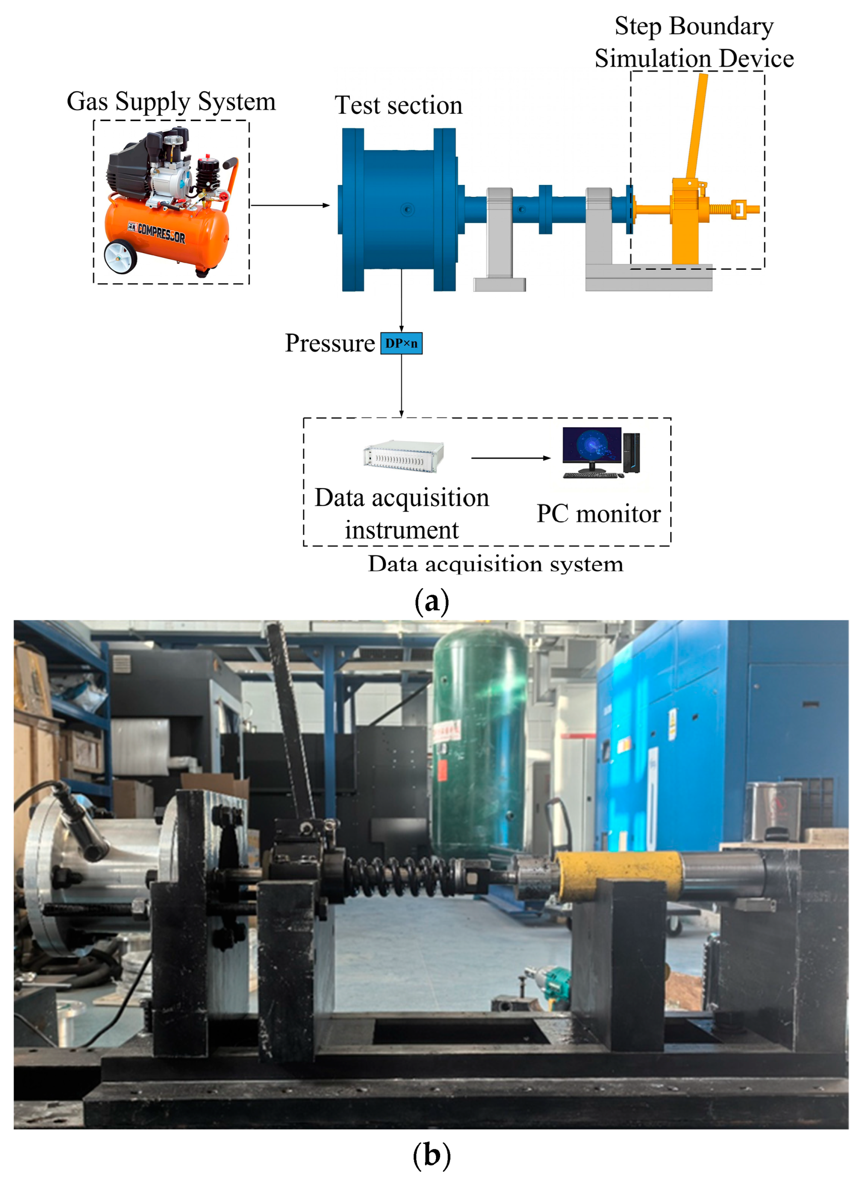
To overcome these limitations, we design and construct a fast transient air-system experimental platform to reproduce cavity venting under abrupt boundary changes. The platform incorporates a repeatable step boundary simulation device to generate rapid boundary opening. Guided by key parameters identified through a dimensionless analysis, we perform fast transient cavity-venting experiments across a range of cavity outlet areas, cavity shapes, and initial pressure ratios. The experiments provide transient measurements of cavity pressure under abrupt boundary changes, revealing how the outlet area, cavity geometry, and initial pressure ratio govern the response. In addition, we simulate the corresponding test conditions using a three-dimensional numerical approach validated against the measurements, providing complementary verification of the influencing factors and their underlying mechanisms. Collectively, this paper establishes a reliable experimental methodology and delivers experimental data to support further studies of fast transient air-system responses.
2. Theoretical Analysis for the Experimental Platform
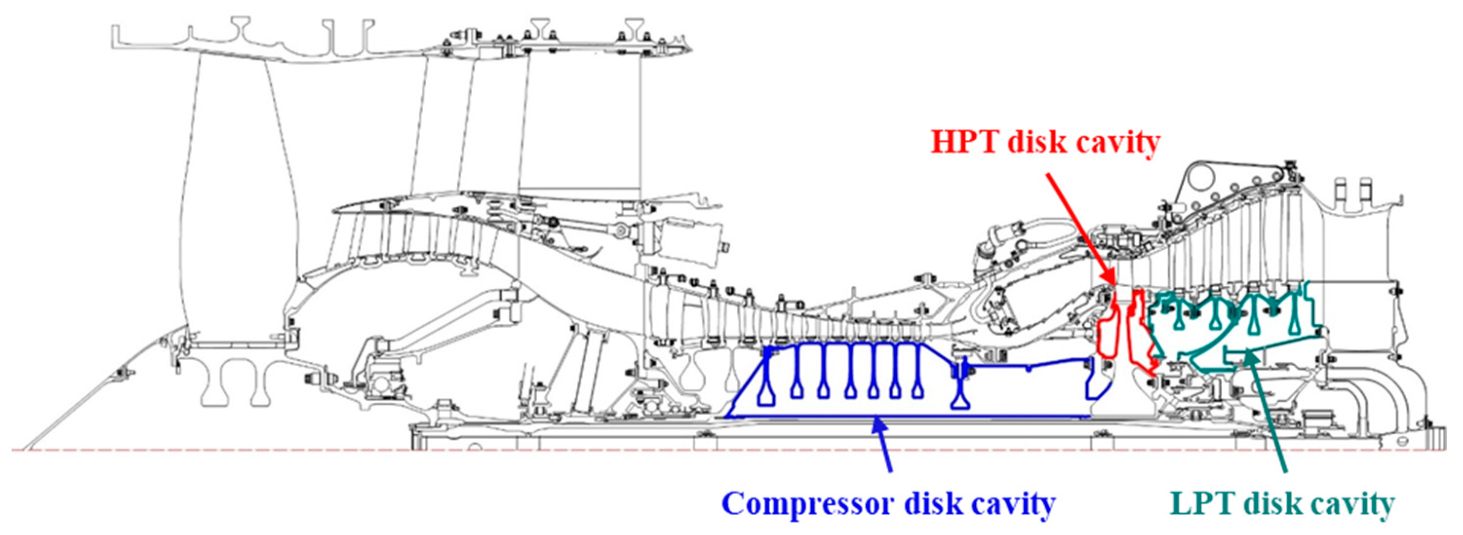
In aero-engine air systems, cavities with relatively large outlet areas are mainly compressor and turbine disk cavities, as schematically shown in
Figure 1. These cavities are axisymmetric; therefore, this paper describes the in-cavity flow using a cylindrical coordinate system
.
,
, and
denote the density, pressure, and temperature, respectively;
denotes the time;
,
, and
denote the dynamic viscosity, specific heat at constant pressure, and thermal conductivity; and
,
, and
are the velocity components in the
,
, and
directions.
To establish similarity criteria for the fast-transient response under step-change boundary conditions, the governing equations are nondimensionalized. The characteristic quantities are chosen as follows:
- (1)
Characteristic lengths: cavity length , cavity diameter , outlet diameter ;
- (2)
Characteristic velocity: the maximum flow velocity ;
- (3)
Characteristic time: ;
- (4)
Characteristic pressure and temperature: initial pressure and initial temperature ;
- (5)
Other flow-property parameters: initial-state , , and .
The dimensionless forms of the variables are defined in Equation (1). The key dimensionless groups include the following:
Reynolds number:
Mach number:
Prandtl number:
Geometric parameters:
The nondimensionalized governing equations can be written as shown below:
- 2.
- 3.
- 4.
Ideal-gas equation of state:
According to standard gas-dynamics relations, the mass-flow rate can be expressed using the flow function
and the aerodynamic function
, as shown in Equations (8)–(10), where
is the dimensionless velocity coefficient. Accordingly, the Reynolds number at the outlet can be rewritten as shown in Equation (11).
The velocity can be expressed in terms of
, as shown in Equation (12); by substituting
, one obtains Equation (13). Using the relations between total and static quantities as expressed in Equation (14), the Mach number can be rewritten as shown in Equation (15).
For the tube exit section, the initial duct pressure is treated as the total pressure , and the ambient pressure is treated as the static pressure . Thus, is governed by the boundary dimensionless pressure ratio , while is governed by and .
To complete the similarity framework, the boundary and initial conditions are also nondimensionalized. In the present process, the boundary change is a step change, and heat transfer is neglected. Therefore, a step-change pressure boundary condition is applied, and no thermal boundary condition is prescribed. The primary initial conditions and the corresponding dimensionless forms are given in Equation (16), and the step-change pressure boundary condition is given in Equation (17).
The dimensionalization introduces the pressure ratio and the temperature ratio . The pressure ratio is already reflected in . In this paper, the initial in-cavity temperature equals the ambient temperature, so is a constant. The derivation ensures kinematic and dynamic similarity; combined with the geometric ratios and , geometric similarity is also satisfied. Because heat transfer is neglected in this experimental campaign, the influence of can be ignored.
From the analysis above, the dependent variables
of the dimensionless governing equations for the fast-transient response under step-change boundary conditions depend on dimensionless independent variables
,
,
,
and the dimensionless groups
,
, and
, as expressed in Equation (18). Under the similarity of the initial pressure ratio, cavities with different geometries become comparable.
has a fixed functional relationship with
and
for the present cavity geometry, as expressed in Equation (19). Therefore, when
is fixed,
is an independent dimensionless group equivalent to
, enabling unified characterization and a comparative analysis of different test specimens.
Based on the dimensionless analysis, experiments are designed to investigate how , , and affect the fast-transient discharge process, extract governing trends, and interpret the underlying mechanisms.
4. Experimental Results and Discussion
4.1. Effect of
Guided by the theoretical analysis, we focus on three dimensionless criteria, which are denoted as
,
, and
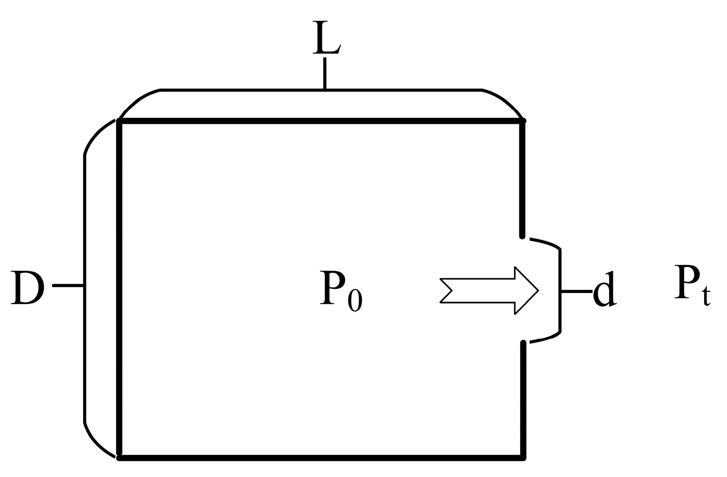
. Specifically, experiments are designed to interrogate how the third dimensionless criterion influences the fast transient venting process of the cavity while the other two criteria are held fixed. The parameters entering the dimensionless criteria are illustrated in
Figure 8, and the selected values of the three dimensionless criteria together with their corresponding experimental conditions are summarized in
Table 3 and
Table 4. In
Table 3,
denotes the cavity outlet area, and
denotes the cavity volume.
Given the limited types and quantities of data available from the experimental measurement points, only qualitative and quantitative assessments of the governing trends can be conducted. To further elucidate the underlying mechanisms, it is necessary to integrate an experimentally validated three-dimensional simulation framework and perform numerical investigations under identical operating conditions for in-depth analysis.
Accordingly, the validated three-dimensional numerical approach reported in Ref. [
12] was adopted. Three-dimensional simulation models corresponding to the experiments were established on the basis of the different geometric parameters and initial pressures listed in
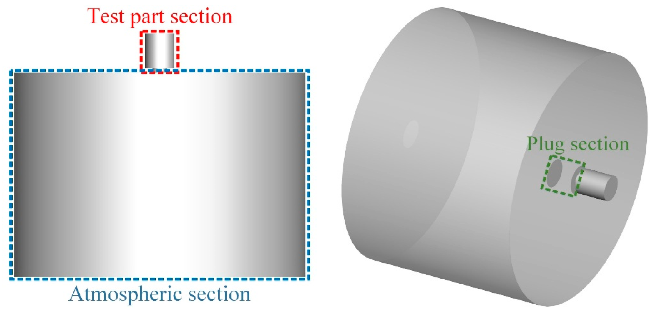
Table 3 and the simulations were then performed, as shown in
Figure 9. All simulations were conducted in ANSYS CFX 2021 with the working fluid treated as an ideal gas. Because the response associated with the fast transient process occurs over an extremely short timescale, wall heat transfer was neglected, and all walls were specified as adiabatic no-slip boundaries. Owing to the small diameter of the interaction interface between the fluid domains, the flow near the cavity port during the simulation resembles a circular jet. According to the study by Kmecova [
16], the SST turbulence model provides high accuracy in the simulation of circular jets. Therefore, the SST turbulence model was given priority, and mesh independence and time-step sensitivity analyses were first carried out before the final turbulence model was confirmed. The entire computational domain was discretized using hexahedral meshes. The cavity fluid domain and the atmospheric fluid domain were each treated using the O-Block partitioning technique, enabling the construction of structured hexahedral meshes over curved surfaces. To capture the flow details in critical regions more accurately, local mesh refinement was applied near the walls and near the interface between the two fluid domains. The height of the first boundary layer was set to 0.001 mm, with a normal growth rate of 1.2, and a smooth transition was maintained between refined and unrefined regions. The initial time step was provisionally set to 1 × 10
−5 s, which is consistent with the sampling frequency of the experimental data.
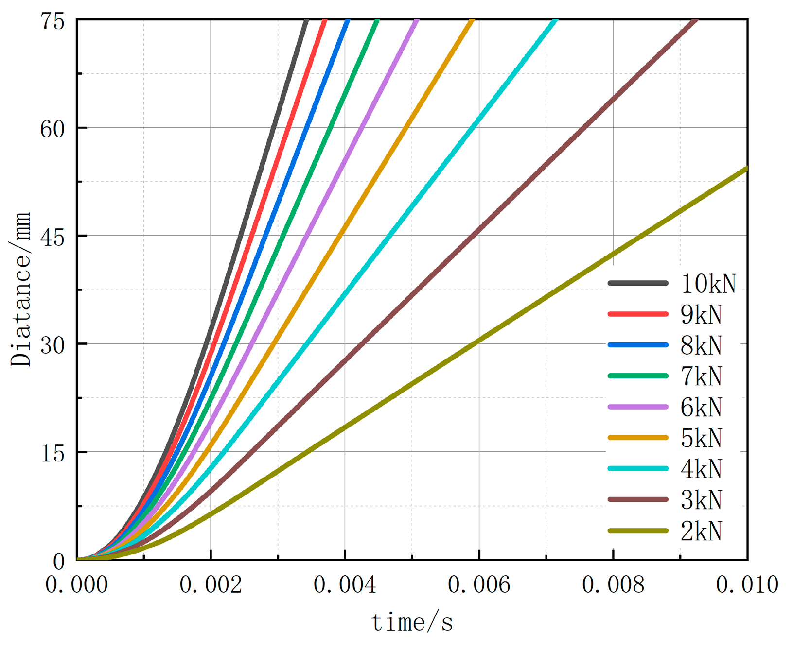
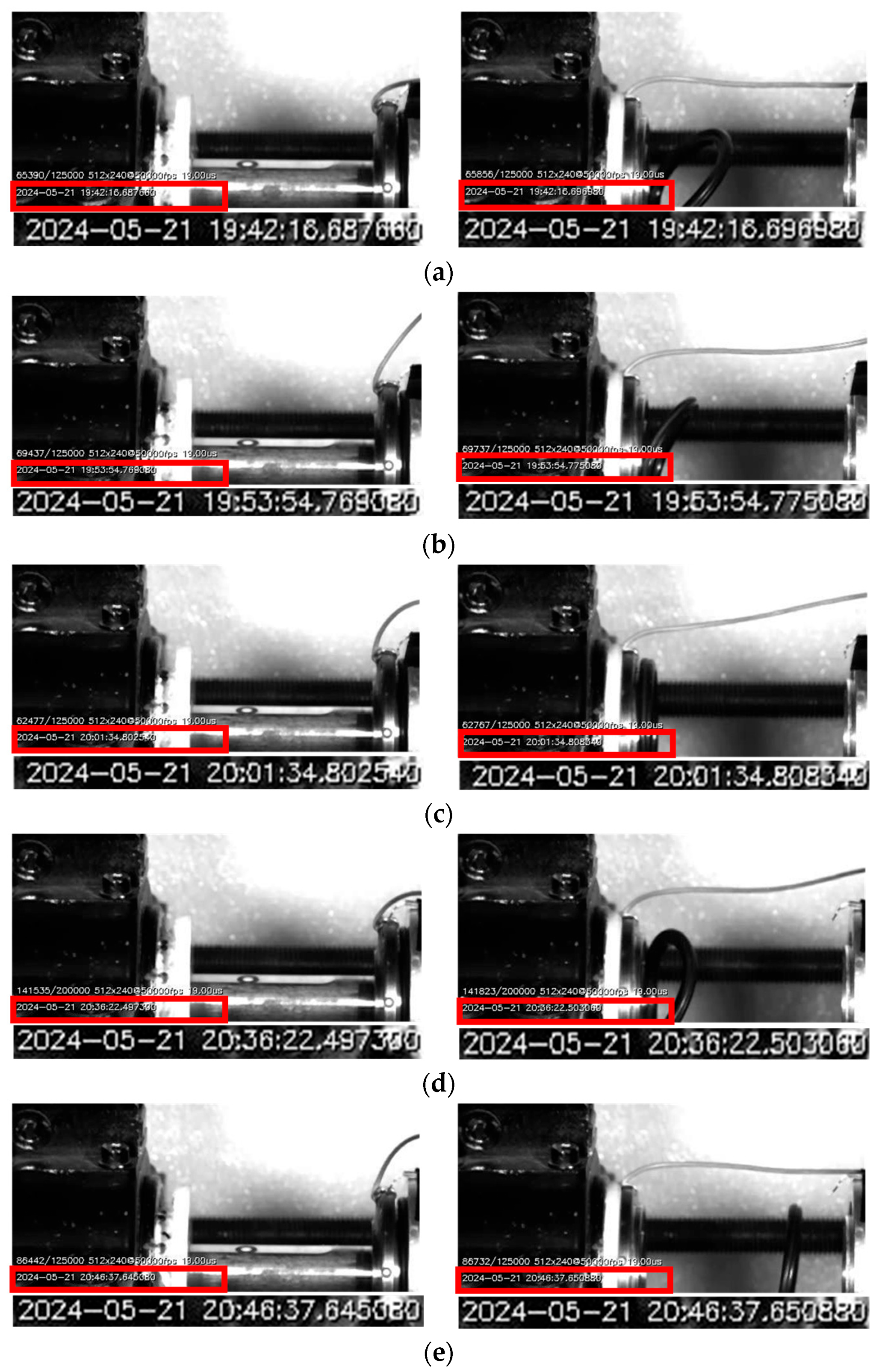
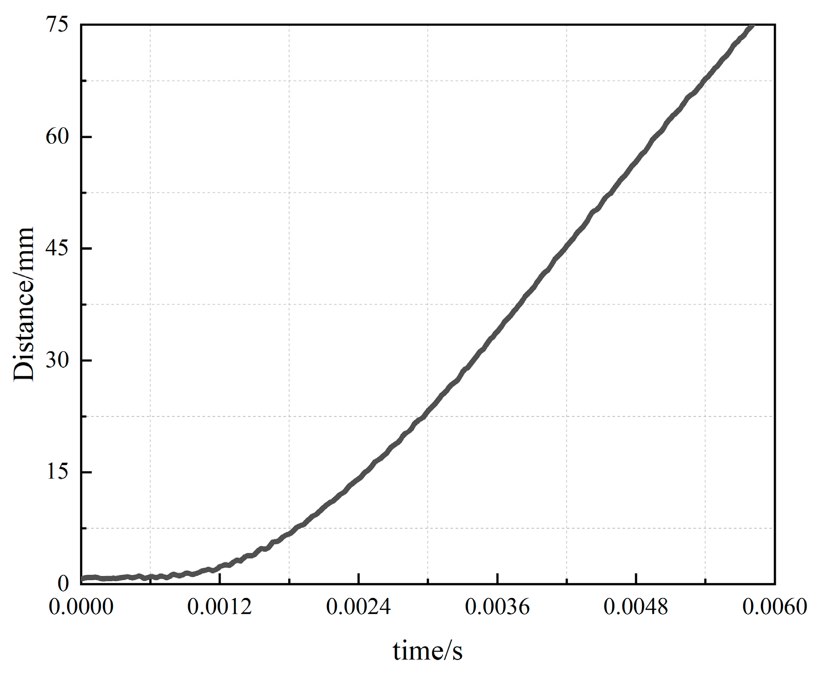
To reproduce the boundary variation observed in the experiments, the displacement of the plug was represented in the three-dimensional model by prescribing the time-dependent position of the plug region. The plug positions at different times were extracted from high-speed camera images, and the corresponding time-varying positional relationship of the plug region was implemented in the three-dimensional model, as shown in
Figure 10. After simulation, the average y+ remained below 1, satisfying the requirement of the SST model. Throughout the calculations, convergence was considered to be achieved when the residuals were generally reduced to the order of 1 × 10
−6.
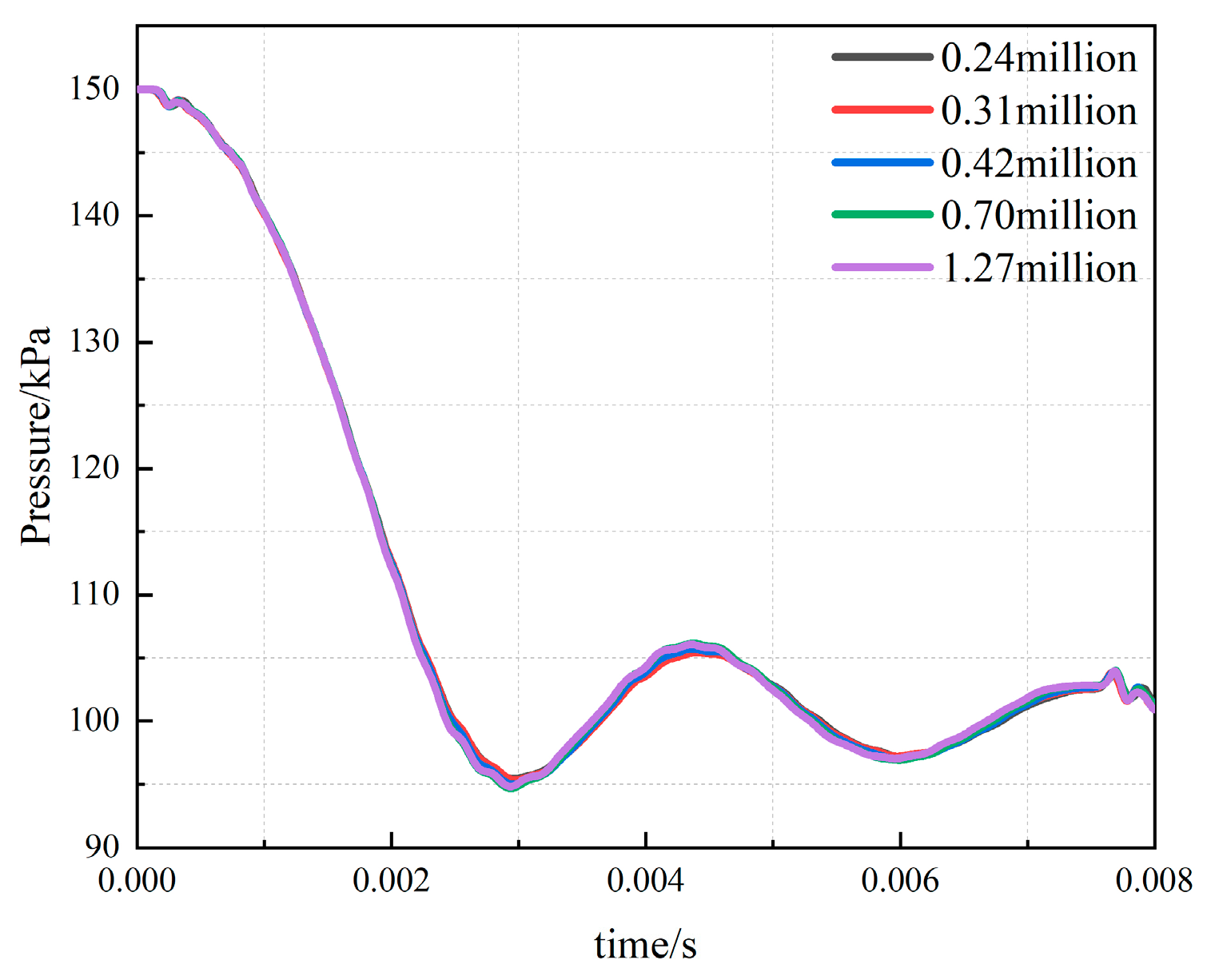
An appropriate mesh resolution was determined through mesh independence verification. Under the condition that y+ satisfied the requirement of the SST turbulence model, the mesh was progressively refined, and simulations were performed using 0.24 million, 0.31 million, 0.42 million, 0.70 million, and 1.27 million cells. Static-pressure monitoring points were arranged in the model according to the pressure measurement locations in the experiments. By comparing the temporal evolution of static pressure at these monitoring points, a suitable mesh resolution was selected. The comparison is presented in
Figure 11. The results indicate that when the mesh number increased from 0.31 million to 1.27 million, the maximum deviation in the simulation results was 1.1%, demonstrating that further mesh refinement had only a minor influence on the predicted results. Therefore, 0.31 million cells were selected for the subsequent simulations. The corresponding mesh distribution is also shown in
Figure 11.
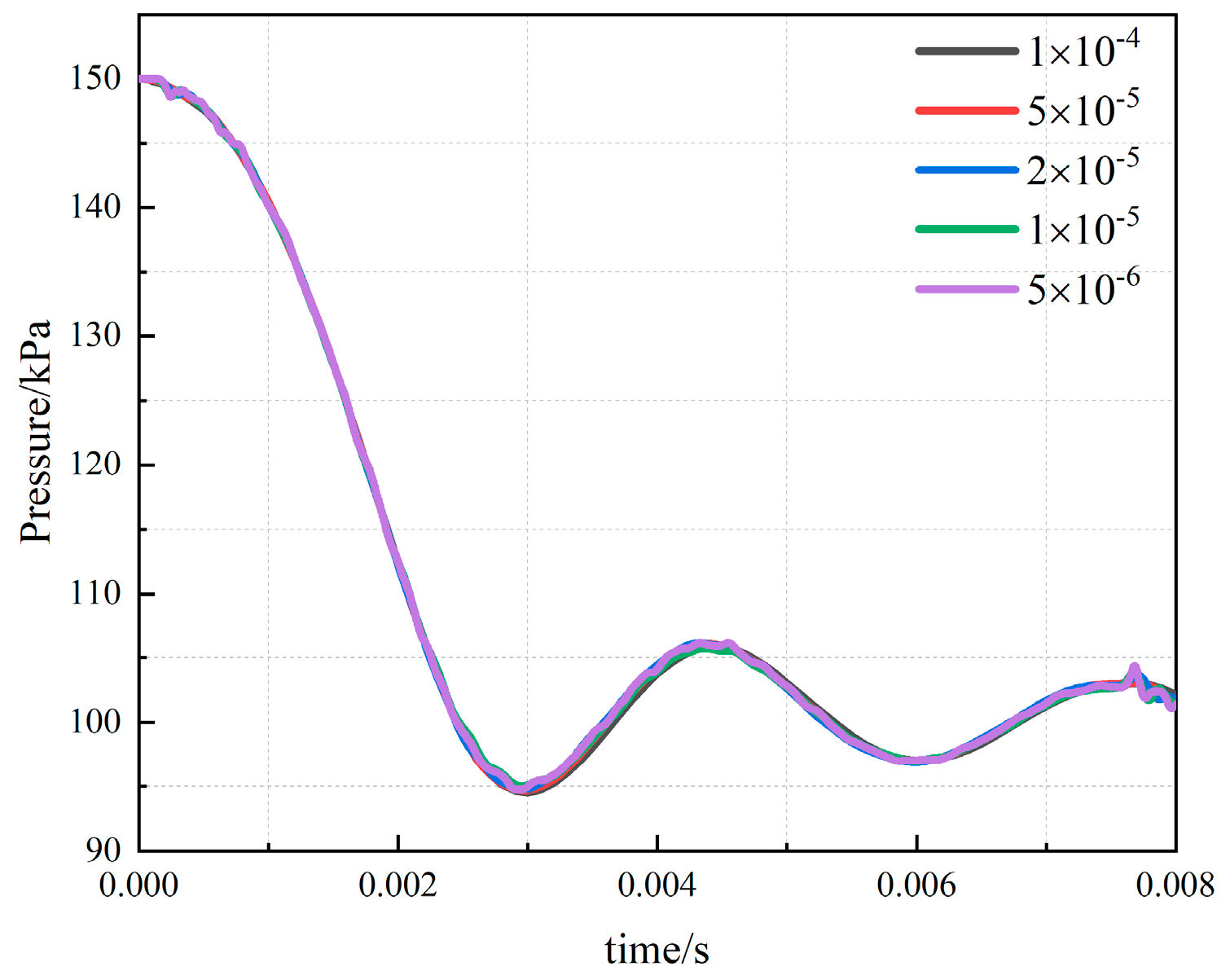
A time-step independence analysis was then carried out using 0.24 million cells. Simulations were performed with time steps of 1 × 10
−4 s, 5 × 10
−5 s, 2 ×10
−5 s, 1 × 10
−5 s, and 5 × 10
−6 s, respectively. The pressure histories at the same static-pressure monitoring points were again compared, as shown in
Figure 12. When the time step decreased from 1 × 10
−4 s to 5 ×10
−6 s, the maximum deviation in the simulation results was 0.7%, indicating that the influence of time-step reduction on the results was limited. Therefore, 1 × 10
−5 s, consistent with the experiments, was selected as the time step for the subsequent study.
Because severe mesh volume variations occur during the displacement of the plug region, other turbulence models were unable to achieve convergence under the same time step and mesh-number conditions during turbulence-model selection. Therefore, the SST model was ultimately adopted for the subsequent study. On the basis of the independence analyses and comparison with the experimental data, the final numerical strategy was established as 0.34 million cells, a time step of 1 × 10⁻⁵ s, and the SST turbulence model, and this strategy was then used for the subsequent numerical investigation.
4.2. Effect of
To examine the influence of
, we compare experiments and simulations across multiple operating conditions listed in
Table 4, while the other two dimensionless criteria are fixed at
and
. The effects of
and
are discussed subsequently. In
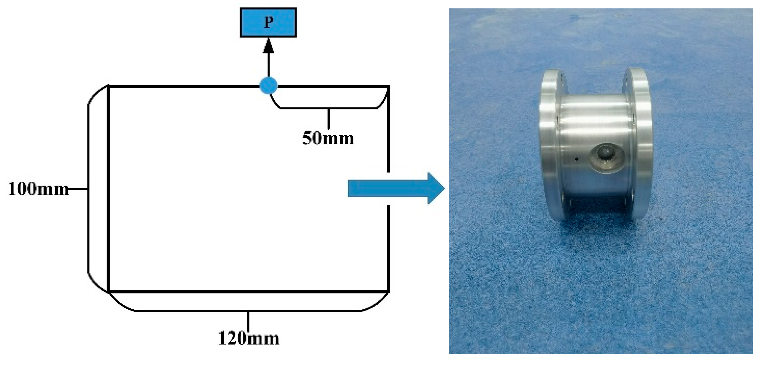
Table 3, the outlet-orifice length is selected as the minimum value that satisfies experimental safety and assembly requirements, as shown in
Figure 13.
Table 4.
Test-specimen parameters for investigating the effect of .
Table 4.
Test-specimen parameters for investigating the effect of .
| Parameter | Value |
|---|
| 1.2 |
| Outlet–hole length/mm | 15 |
| 1.5 |
| Outlet diameter /mm | 10 | 20 | 30 | 40 | 50 |
| 0.008 | 0.033 | 0.074 | 0.131 | 0.204 |
The locations of the pressure measurement points are shown in
Figure 13. To facilitate a consistent comparison of the static-pressure response histories under different values of the dimensionless criterion
, the static pressure at measurement point
is cast into a dimensionless form according to Equation (21), where
denotes the initial cavity pressure and
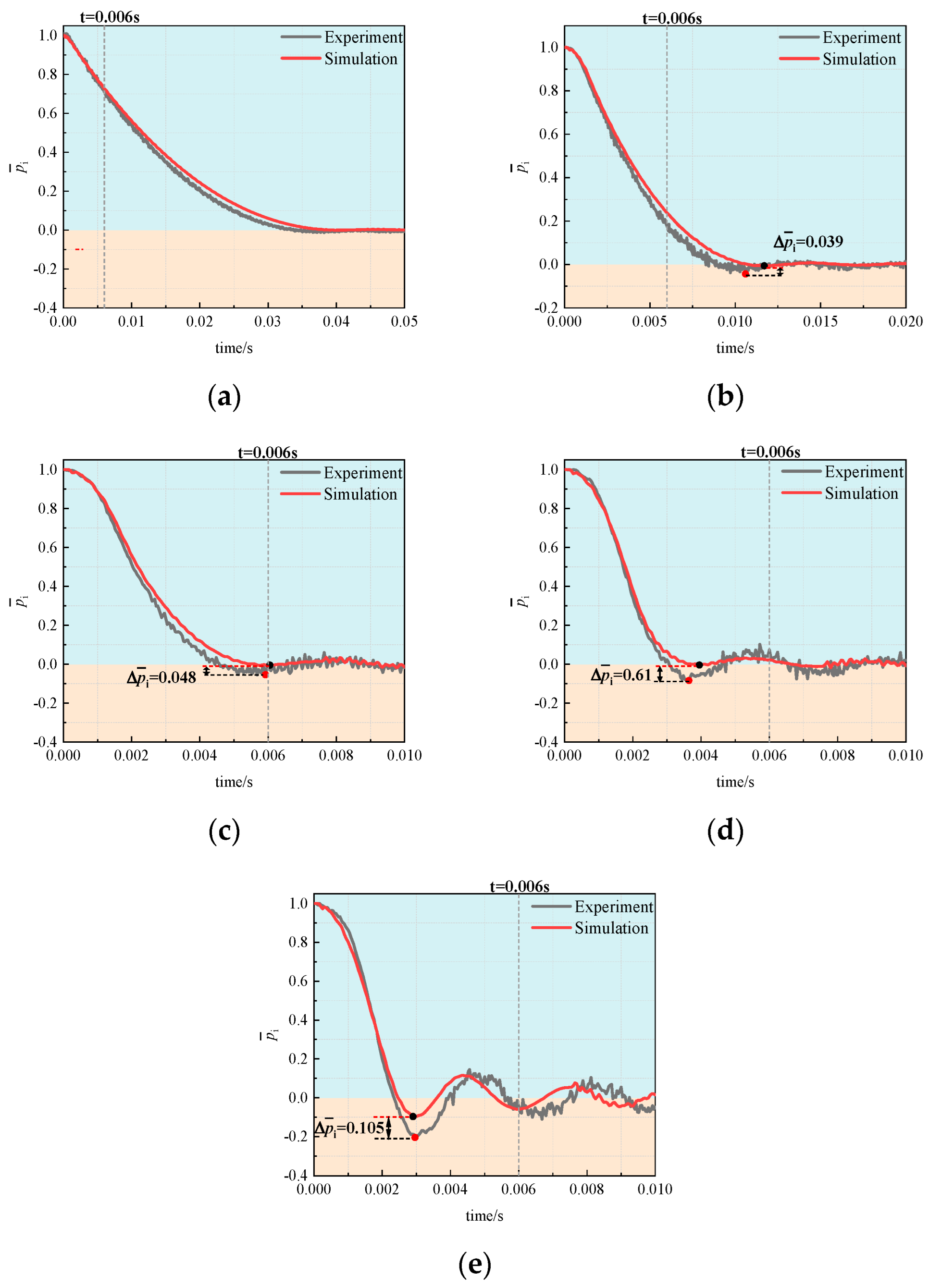
denotes the ambient pressure. A direct comparison between the experimental measurements and the three-dimensional simulation results is presented in
Figure 14. In this figure,
represents the time required for the plug to complete its prescribed motion.
Both the experiments and the simulations show that at a fixed value of
, the pressure signal
decreases in an approximately monotonic manner and eventually approaches a steady state. As
increases, the pressure drop within the cavity accelerates, and pronounced pressure oscillations emerge. With further increases in
, the oscillation amplitude increases while the oscillation period decreases, as quantified in
Table 5.
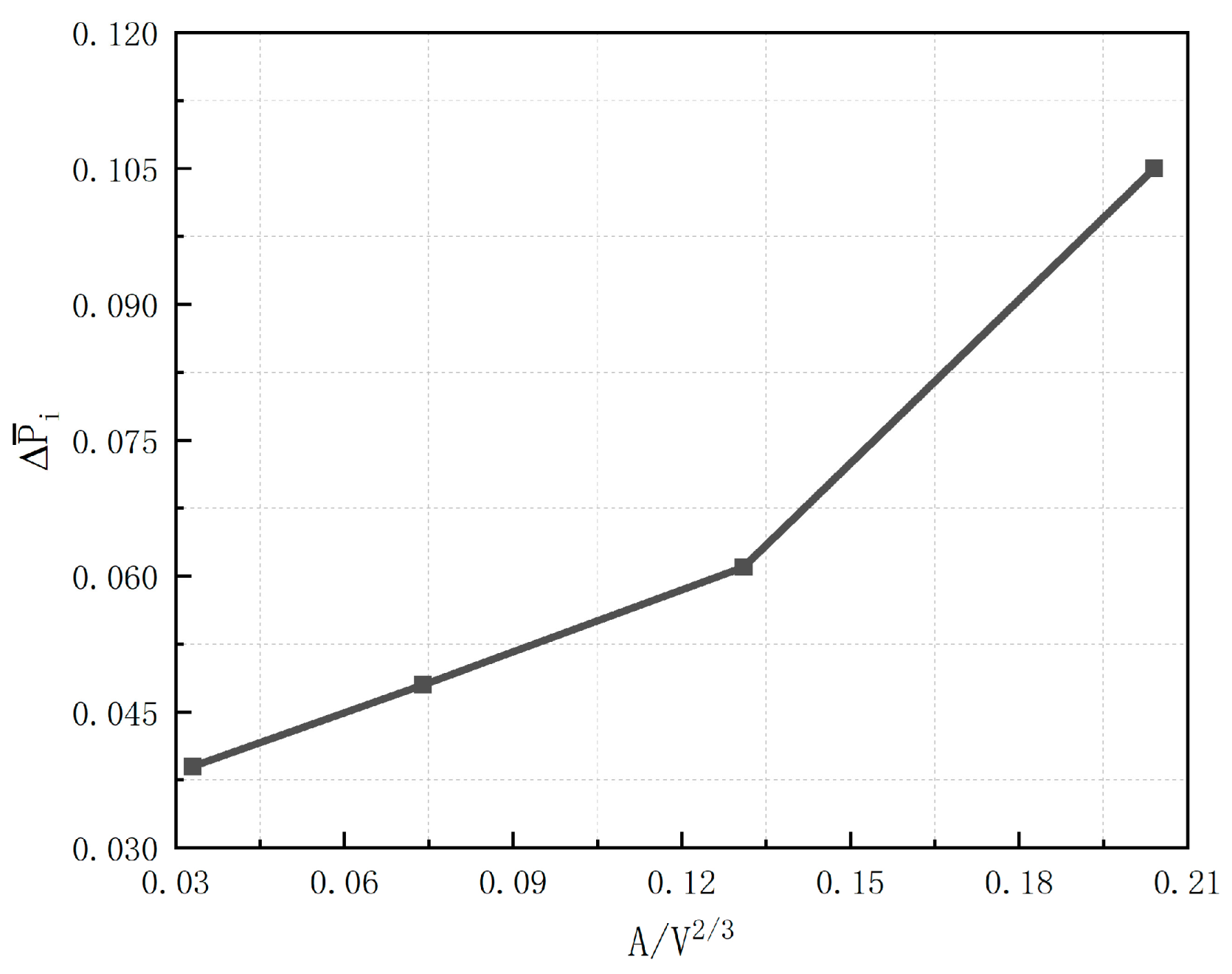
However, a comparison between the three-dimensional simulations and the experimental results under identical operating conditions shows that the simulated pressure-oscillation amplitudes are consistently smaller than those measured experimentally, and the discrepancy increases with increasing
. The variation in
with
is shown in
Figure 15, where
exhibits an approximately linear dependence on
. This trend indicates that the deviation is likely dominated by a single factor. Under conditions where the influence of plug motion must be considered, the deviation is attributed to the plug motion.
For condition
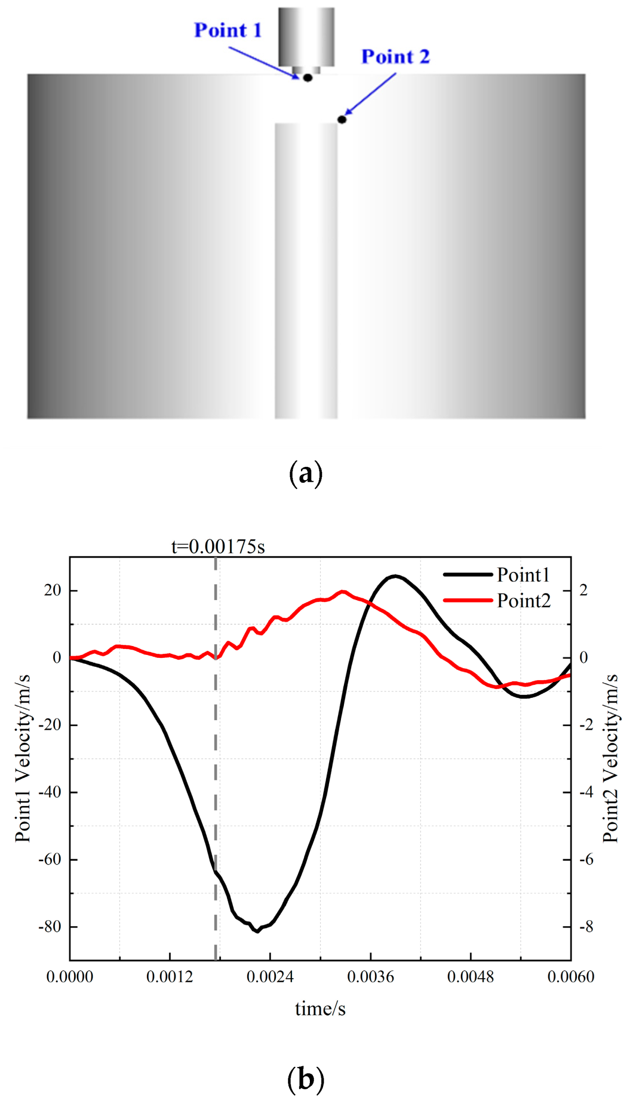
, a three-dimensional model was selected, and monitoring points were arranged as illustrated to track the axial gas velocity at the cavity outlet and in the vicinity of the plug during the simulation. The corresponding results are presented in
Figure 16. The axial velocity at Point 2 follows a trend broadly consistent with that at Point 1, but it exhibits a distinct temporal lag. Specifically, the onset of a pronounced change in axial velocity at Point 2 is delayed by 0.00175 s relative to Point 1. A preliminary interpretation is that after the plug begins to move, the gas near the plug remains initially stagnant. Only after the flow perturbation from the cavity outlet propagates to the region near the plug does the local gas undergo appreciable acceleration. This behavior indicates that in the three-dimensional simulation, representing plug motion solely through wall displacement cannot capture the entrainment imposed on the surrounding gas. In the experiment, by contrast, plug motion induces ambient gas movement, and the ambient flow in the discharge direction further enhances the cavity outflow to a certain extent. Consequently, although the pressure response in the experiment and simulation remains largely consistent in phase, the experimental response exhibits a greater amplitude. Therefore, the three-dimensional simulation results are most appropriately used for qualitative interpretation and as support for mechanistic analysis.
Building on the conclusions of Ref. [
12] and the flow-driving mechanism, we analyze how increasing
affects the static pressure at the measurement point. When a pressure difference exists between the cavity and the ambient environment, the gas near the outlet accelerates outward under the pressure-gradient driving force. As the cavity pressure approaches the ambient level, the accelerated gas cannot be brought to rest instantaneously; instead, it continues to discharge due to inertia, causing a pressure “overshoot”; i.e., the cavity pressure temporarily drops below the ambient pressure and thereby initiates pressure oscillations. Increasing
enlarges the region of gas accelerated during the pressure-driven stage, increases the mass of gas that still carries momentum in the inertia-dominated stage, and thus increases both the inertially driven discharged mass and the oscillation amplitude. Meanwhile, a larger outlet area accelerates the overall flow and shortens the oscillation period.
4.3. Effect of
On the basis of this analysis, we select the outlet-area condition
and investigate the influence of the length-to-diameter ratio
on the pressure response. The corresponding geometric parameters are listed in
Table 6. The associated experiments are conducted, and the corresponding three-dimensional models are established for simulation. The static-pressure data at the measurement point are processed in dimensionless form following Equation (21).
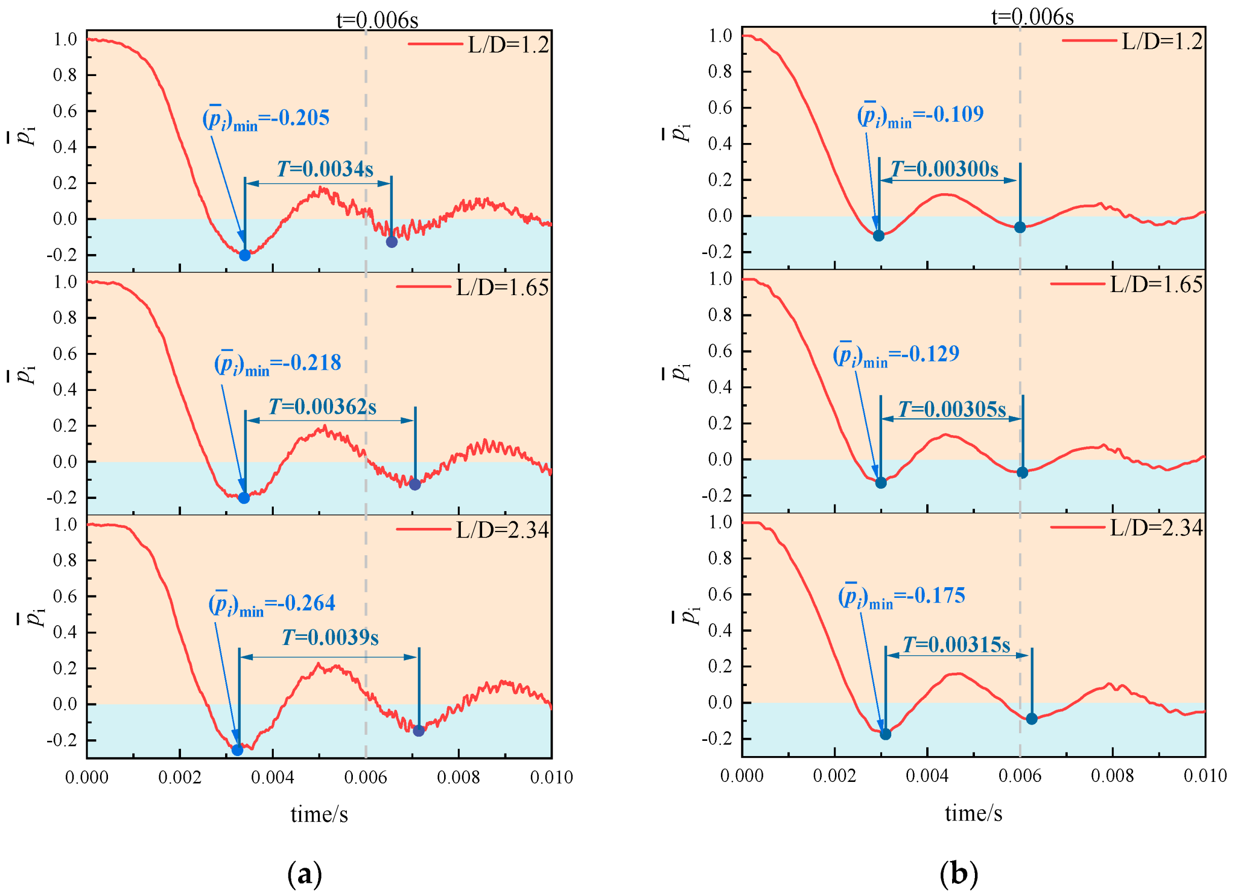
Figure 17 compares the static-pressure histories at the measurement point obtained from experiments and three-dimensional simulations under condition
. As
increases, both the oscillation amplitude and the oscillation period increase. When
is increased from 1.2 to 2.34, the minimum dimensionless pressure at the measurement point decreases from −0.205 to −0.264 (a reduction of 28.8%), while the oscillation period increases from 0.0034 s to 0.0039 s (an increase of 41.7%). A preliminary interpretation is as follows: with
held constant and inertial effects being relevant, increasing
lengthens the axial propagation distance, thereby increasing the travel time of pressure disturbances and enlarging the oscillation period. Consistent with Ref. [
12], a larger
also intensifies inertial effects within the cavity, increasing the mass of gas discharged under inertia and thus amplifying the pressure oscillations. The three-dimensional simulations are further used to verify these explanations.
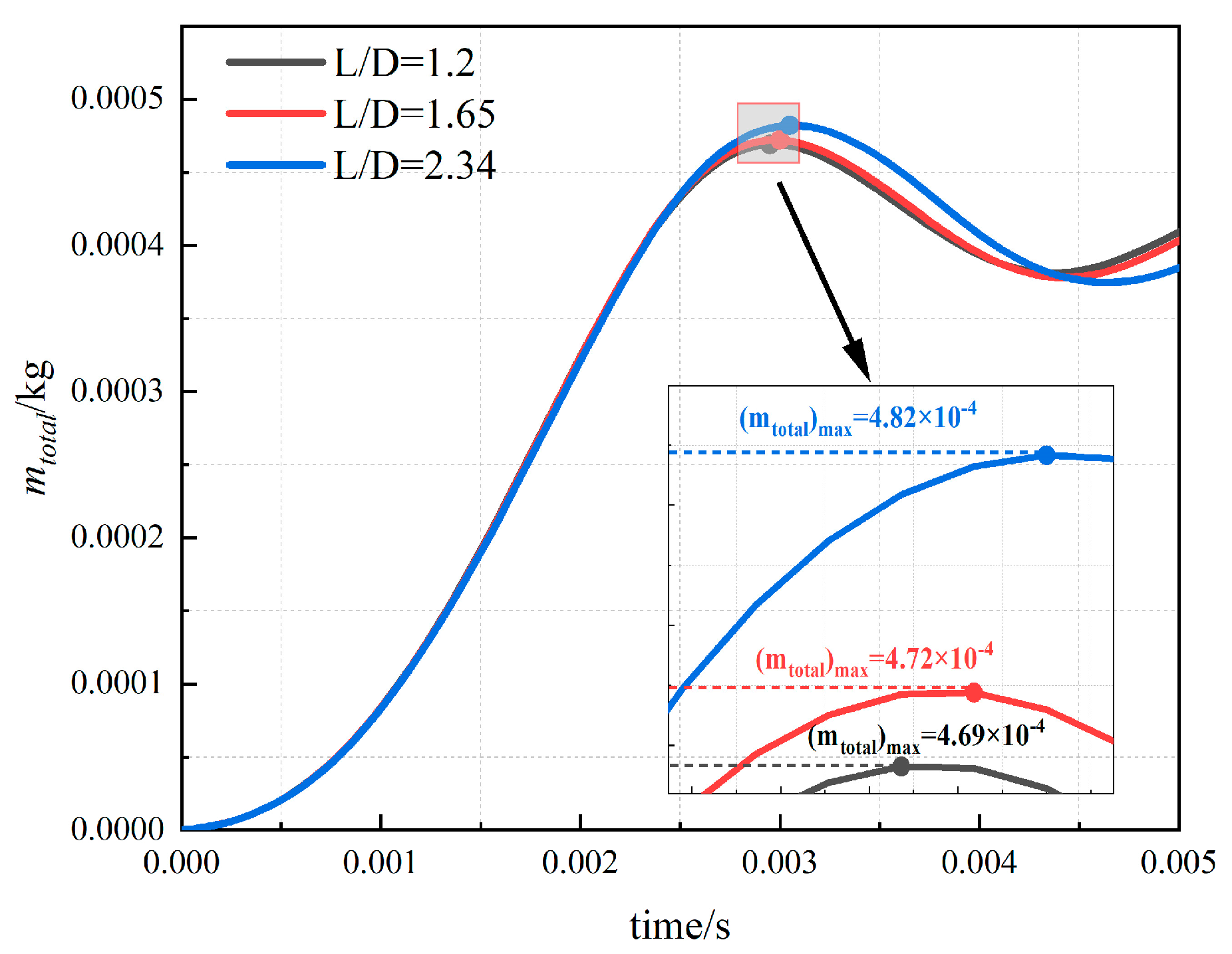
Figure 18 compares the evolution of the total amount of gas discharged from the cavity
under different values of
. As
increases,
rises during the venting process: when
is increased from 1.2 to 2.34,
increases from 4.69 × 10
−4 to 4.82 × 10
−4. The increase in
directly lowers the minimum pressure attained within the cavity and amplifies the pressure-oscillation magnitude. In addition, the onset of
is delayed as
increases.
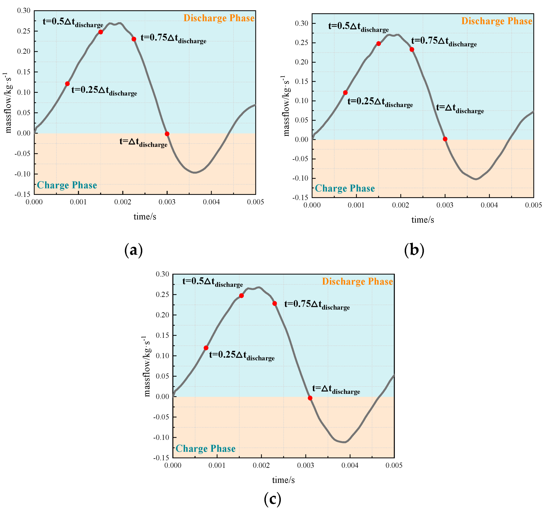
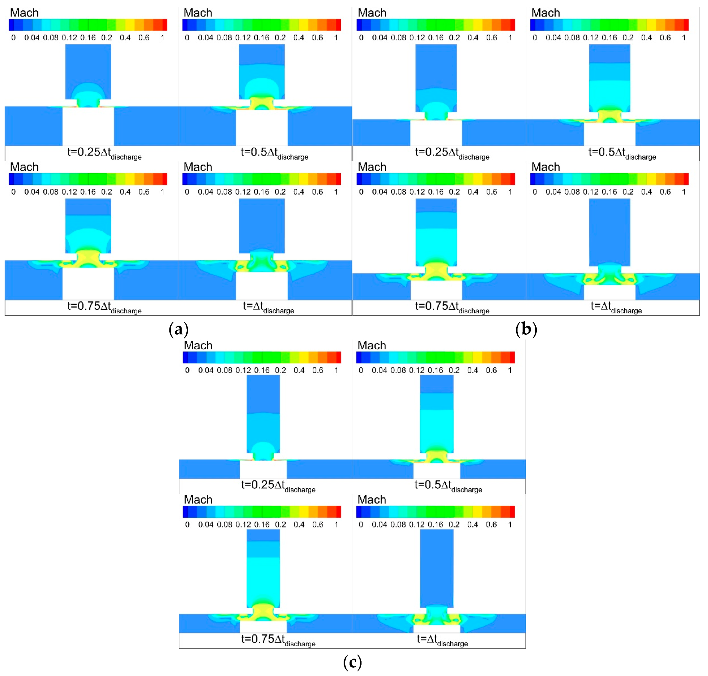
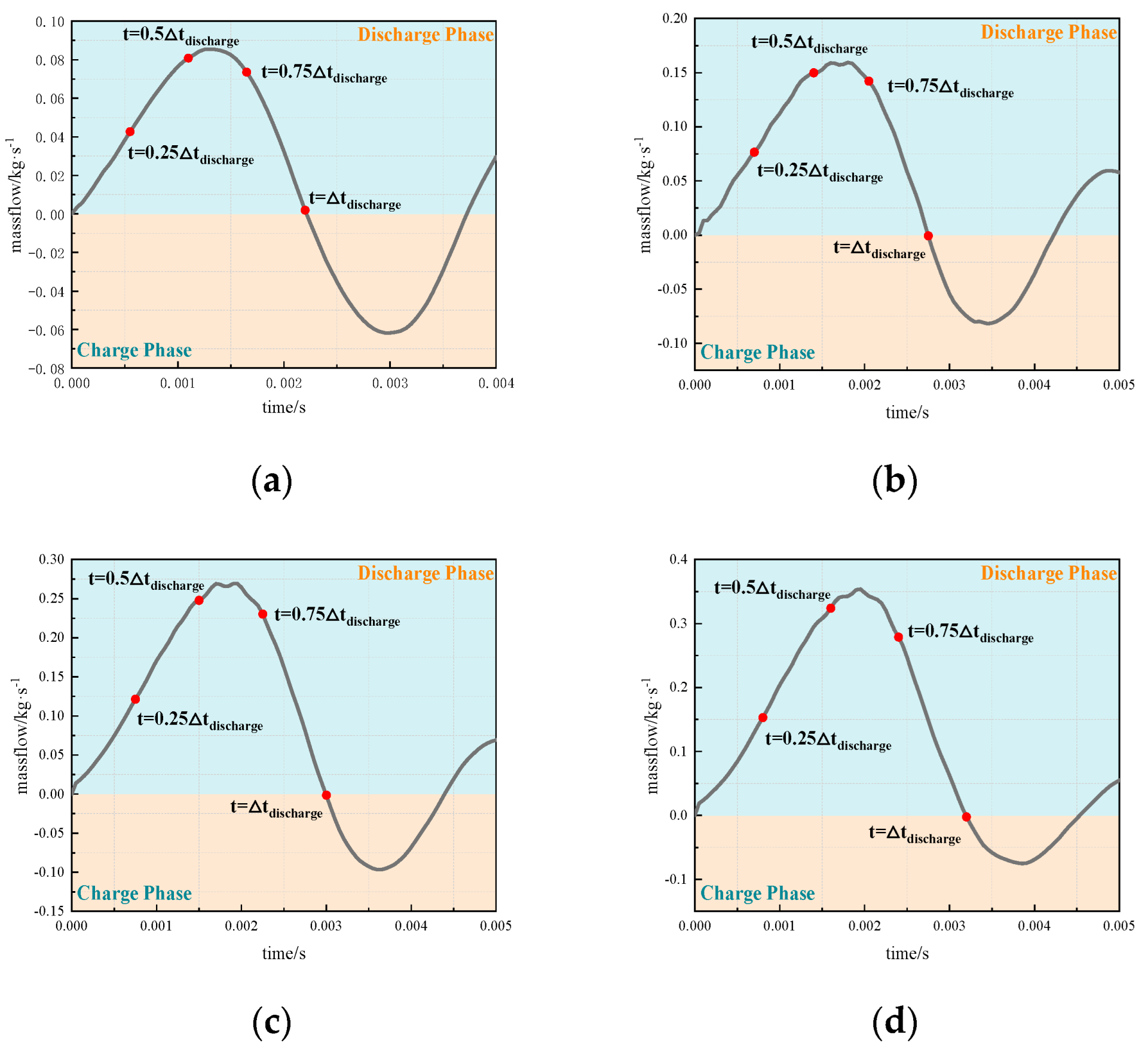
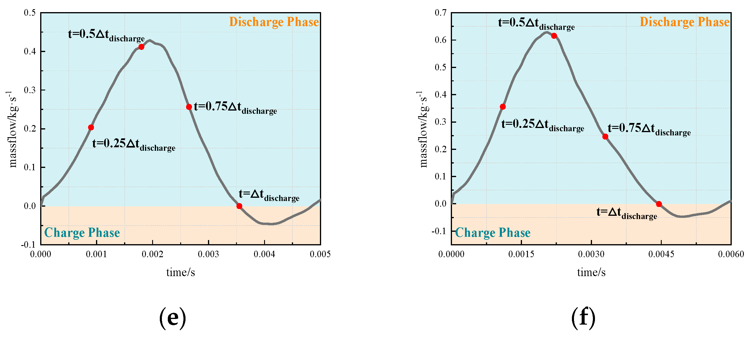
Figure 19 delineates the venting and refilling stages of the cavity based on the time evolution of the outlet mass flow rate. To compare how the internal flow field develops under different values of
, several representative instants within the first venting stage are selected, and the corresponding velocity-field distributions inside the cavity are juxtaposed in
Figure 20.
According to the analysis presented in
Figure 20, during the charge and discharge processes of the cavity, an increase in
enlarges the region occupied by flowing gas within the cavity at the corresponding moments of the discharge process. As a result, the influence of inertial forces inside the cavity is strengthened, leading to an increase in the gas mass discharged from the cavity under inertial-force-driven motion during discharge, thereby causing
to increase. A comparison of the gas mass discharged from the cavity during the discharge process under different
conditions is provided in
Table 7. Here, C denotes the gas mass at the steady state, and
represents the difference between
and
—namely, the gas mass discharged from the cavity under inertial-force-driven motion in the absence of a pressure difference. The data in the table show that as
increases from 1.2 to 2.34,
increases from 3.6 × 10
−5 kg to 4.9 × 10
−5 kg, corresponding to an increase of 36.1%. This analysis demonstrates that an increase in
enhances the influence of inertial forces within the cavity, thereby increasing the gas mass discharged from the cavity under inertia-driven motion and ultimately amplifying both the amplitude and period of pressure oscillation, which is in agreement with the preceding analysis.
4.4. Effect of
Building on the trends identified above for the effect of increasing
on the fast transient venting response of the cavity, we select—among the existing test geometries—the configuration
that exhibits the strongest inertial influence within the cavity, and then we investigate how the initial pressure ratio
governs the fast transient response during cavity venting. Because air is used as the working gas in the present experiments, the critical pressure ratio is 1.89, and the tested conditions therefore include supercritical pressure ratios. The experimental matrix is summarized in
Table 8. Corresponding three-dimensional models are also constructed based on the parameters in
Table 8 to perform the simulations.
The static pressure at the measurement point is rendered dimensionless using Equation (22), where
is taken as the ambient pressure for each individual test.
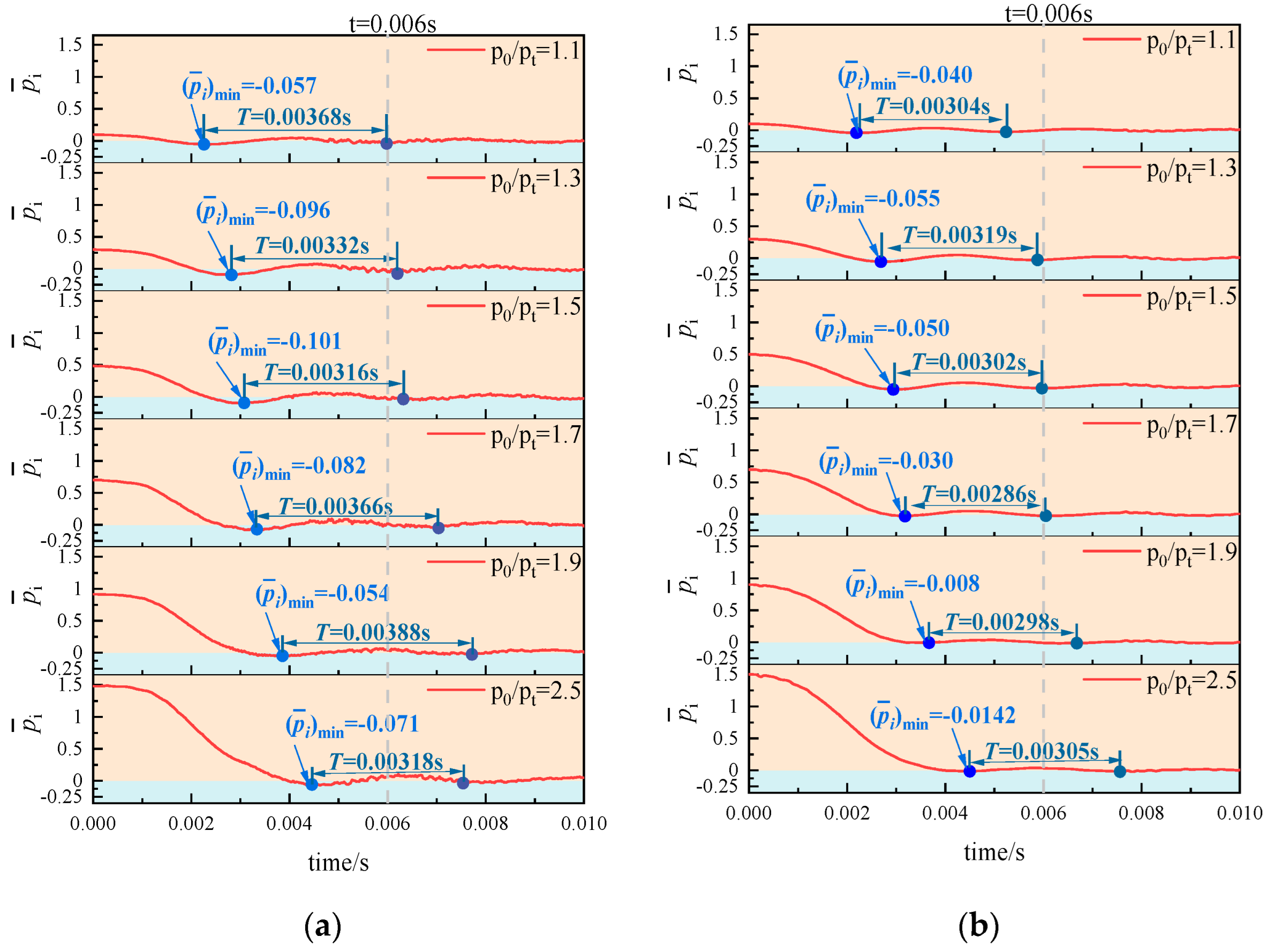
Figure 21 compares the evolution of
at the pressure-measurement location between the experiments and the simulations under different values of
. As
increases, both datasets exhibit broadly consistent, yet distinctly nonlinear, variations in the pressure-oscillation amplitude. Within regime
, the oscillation amplitude increases with
; within regime
, it instead decreases as
increases; and in regime
, a modest increasing trend re-emerges with further increases in
. Overall, the influence of
on the oscillation amplitude and period is not monotonic, suggesting a coupled, multi-factor interplay involving
and the plug-motion history. We therefore leverage the three-dimensional simulations for further mechanistic interrogation.
The temporal variation in the cavity outlet mass flow rate is used to distinguish between the venting and refilling stages, as illustrated in
Figure 22. Because our focus is the oscillation amplitude during the first pressure-drop event, we define the duration of the first venting stage as
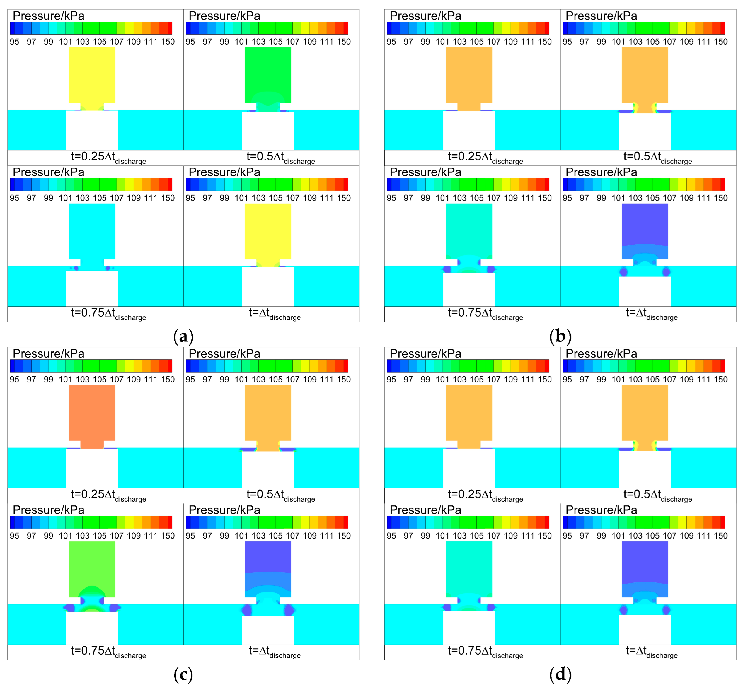
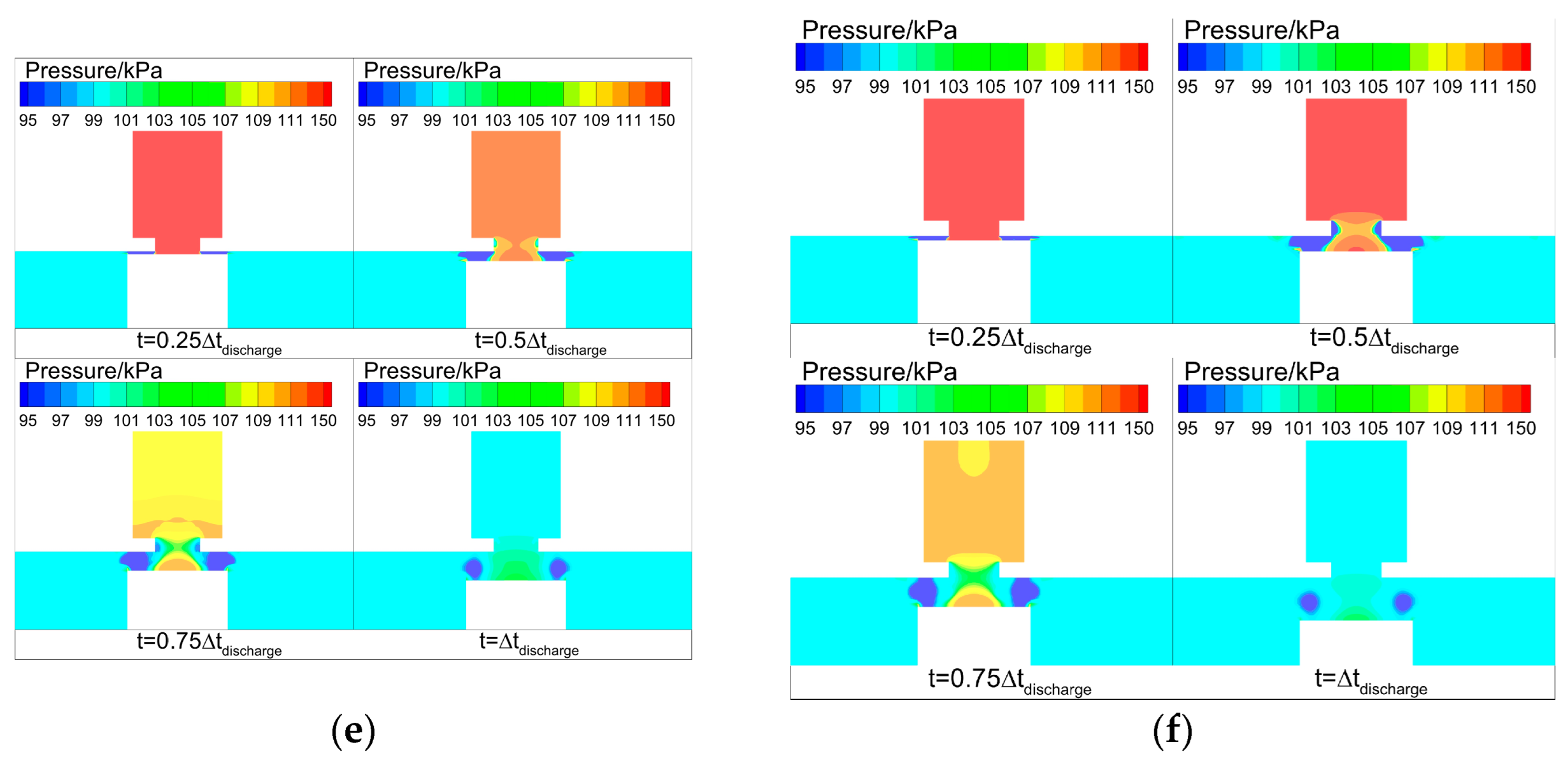
. Representative instants within this venting stage are then selected to compare the plug position and the corresponding evolution of the flow field, as depicted in
Figure 23.
To interpret the nonlinear dependence of the pressure-oscillation amplitude and period on , we account explicitly for the plug-motion history. In general, increasing simultaneously raises the peak discharge velocity and prolongs the pressure-drop process. In stage , the pressure drop is short; gas acceleration within the orifice and the discharged mass remain limited, and a sufficiently strong localized high-pressure region does not develop near the cavity inlet and outlet to suppress outflow. In this regime, the dominant control on discharge is the distance between the plug and the cavity inlet and outlet. Accordingly, as increases, the pressure-drop duration increases and the plug moves farther from the cavity, weakening the suppression of outflow; the oscillation amplitude increases, whereas the period decreases. In stage , increasing further extends the pressure-drop duration, and the high-velocity discharge together with the external jet establishes a localized high-pressure region between the cavity inlet and outlet and the plug. Because the plug is already relatively distant from the cavity inlet and outlet, this localized high-pressure region becomes the primary factor governing the discharge. As increases, the localized high-pressure region intensifies, leading to a reduced oscillation amplitude and an increased period. When reaches stage , the localized high-pressure region diminishes with increasing , lowering its ability to suppress discharge; consequently, the oscillation amplitude increases again and the period decreases.
Further analysis was conducted using the total outlet mass flow rate under different
conditions. Specifically, the steady total outlet mass flow rate
and the maximum total outlet mass flow rate
were compared, and their difference was defined as
, which represents the gas mass discharged from the cavity under inertial-force-driven motion in the absence of a pressure difference. The comparison is summarized in
Table 9. The data indicate that as
increases from 1.3 to 1.9,
decreases from 3.84 × 10
−5 kg to 1.57 × 10
−5 kg, corresponding to a reduction of 59.11%. With increasing
, the gas mass discharged from the cavity under inertial-force-driven motion decreases. This finding confirms that a suppressive effect on the outflow exists in this stage, consistent with the preceding analysis, and further verifies the presence of a local high-pressure region that inhibits the outflow.