An Analysis of the Thermomechanical Behavior of a Solid Electroconductive Cylinder Subjected to an Amplitude-Modulated Radio Impulse

Abstract

A physical and mathematical model is proposed that takes into account the sequential interaction of electromagnetic, temperature, and mechanical fields to assess the thermostressed state of an electroconductive body and predict its load-bearing capacity under the action of an external non-stationary electromagnetic field. Initial-boundary problems are formulated to determine the parameters of the electromagnetic field, temperature, dynamic thermoelastic stresses, and their intensities in a long, solid, non-ferromagnetic electroconductive cylinder. Based on the Huber–von Mises criterion, an assessment of the load-bearing capacity of this cylinder is proposed. A numerical analysis of Joule heat, ponderomotive force, temperature, components of the dynamic stress tensor, and their intensities in a solid stainless-steel cylinder under the action of an amplitude-modulated radio pulse is performed. The limiting values of the amplitude–frequency characteristics and the duration of the electromagnetic action, at which the cylinder under consideration retains its load-bearing capacity as a structural element, have been established.

1. Introduction

Induction heating is one of the most environmentally friendly and energy-efficient methods of heat treating materials, as it is based on the action of an electromagnetic field (EMF) generated by an alternating electric current. For industrial applications, induction heating typically uses stationary electromagnetic fields with a carrier frequency in the range of $\omega =$ 5–16 kHz. The use of EMFs at such frequencies allows for the continuous heating of electrically conductive workpieces, especially those with cylindrical geometry, to relatively high temperatures (approximately 100–1000 °C). These temperatures are achieved through the efficient transfer of electromagnetic energy to the workpiece due to the phenomenon of electromagnetic induction, where induced currents are converted into thermal energy. Physical and mathematical models are commonly used to analyze temperature regimes in electroconductive workpieces during induction heating. These models are based on the coupled solution of Maxwell’s electrodynamics equations and Fourier’s heat conduction equation. In this formulation, Joule heat generated by induced currents acts as a heat source in the heat conduction equation. Estimating the volumetric density of Joule heat allows for predicting the energy consumption of induction heating devices.

A brief overview of the physical principles and practical application of induction heating technologies is presented in reference [1]. It summarizes the fundamental properties of heated materials and discusses metallurgical processes associated with electromagnetic heating, including surface hardening, tempering, stress relief, and annealing.

There are two main heating methods—resistive and induction heating—that are used for heat transfer in heat pipes. In particular, Ma et al. [2] conducted experiments on starting a sodium heat pipe using resistive heating. However, due to the difficulty of achieving low thermal resistance between the resistive heating source and the heat pipe in practice, as well as the difficulty of effectively controlling heat leakage, it turned out to be difficult to load a large heat flux onto heat pipes using such heating. It has been established that resistive heating is not suitable for conducting heat transfer limit tests for heat pipes with high thermal conductivity. At the same time, induction heating, due to its advantages such as high efficiency and a high heating rate compared to resistive heating, is extremely suitable for testing heat pipes with high heat load requirements [3]. The authors have developed a thermoelectrically coupled model using finite elements based on a pseudo-Gnito model of thermal conductivity and electromagnetic theory. Quantitative calibration formulas for induction heat are established depending on frequency, current, and temperature using two sets of quadratic polynomial approximations.

Some studies were devoted to temperature regimes in electrically conductive cylindrical billets made of non-ferromagnetic materials, such as metals, their alloys, and graphite rods, which have important practical applications, including use in nuclear reactors. In particular, ref. [4] proposes an analytical solution to a multiphysical model describing the induction heating of graphite cylinders using the multiscale perturbation method. The analytical results obtained were compared with finite element modeling and experimental modeling of an alternating current circuit of an induction heating power source.

Another area of research concerns the design and optimization of zone induction heating devices. Multi-inductor systems with continuous feeding of workpieces are considered particularly promising, as they allow for maintaining an almost constant average temperature across the entire cross-section of the workpiece. In [5], a numerical model was developed to analyze the related electromagnetic and thermal processes in metal workpieces for the design of zone induction heating devices and the selection of optimal heating parameters. The study presents three-dimensional distributions of electrical conductivity and relative magnetic permeability inside a moving steel workpiece, as well as temperature distributions along its length for different inductor power coefficients.

An analytical approach to solving a non-stationary heat conduction problem in a three-dimensional cylindrical body subjected to induction heating is proposed in [6]. In this study, Maxwell’s equations were simplified to determine the internal distribution of current density, which allows for an analytical description of heat generation inside the cylinder. The temperature field was obtained by solving the unsteady heat conduction equation using Green’s functions. In addition, the authors proposed an algorithm that takes into account the temperature-dependent thermophysical properties of the material. The theoretical results were verified by comparison with experimental data obtained under similar conditions. In the studies analyzed above, induction heating was carried out using steady sinusoidal time-varying electromagnetic fields.

With the rapid development of the latest technologies for the pulsed thermal treatment of materials, pulsed electromagnetic fields have begun to be widely used [7,8]. In modern pulsed induction heating technologies, such non-stationary electromagnetic fields with sinusoidal oscillations modulated by pulsed signals [9,10,11] began to be used. The use of such non-stationary EMFs allows for taking into account the moments of current switching in the inductor, which significantly affects the heating process. In addition to the above-mentioned pulsed fields, quasi-steady electromagnetic fields are also used in induction heating technologies [12].

The use of pulsed electromagnetic fields with different time profiles in modern technological processes is discussed in the monograph [13]. The features of magnetic pulse processing of metals in industrial technologies are described in [14], and the fundamental principles of electromagnetic processing of electrically conductive materials are presented in [11].

The action of electromagnetic fields on electroconductive bodies causes the occurrence of related electromagnetic, thermal, and mechanical processes. In particular, electroconductive bodies can be polarized or magnetized under the action of electromagnetic excitation. In particular, ref. [15] considers mathematical models describing such related processes in electroconductive bodies subjected to high-frequency induction heating, taking into account the temperature dependence of the physical and mechanical characteristics of the material.

Research into the thermally stressed state of electroconductive bodies during induction heating by steady and quasi-steady electromagnetic fields was conducted on the basis of a quasi-static thermomechanics problem for electroconductive bodies [16,17,18].

Dynamic thermoelastic processes in electroconductive solids under the action of pulsed electromagnetic fields are not sufficiently covered in the literature. In particular, ref. [19] investigates dynamic thermoelastic processes in an electroconductive non-ferromagnetic plate subjected to micro- and nanosecond electromagnetic pulses. A physical-mathematical model describing dynamic thermoelastic processes in non-ferromagnetic electroconductive bodies under the action of electromagnetic fields with a pulsed modulating signal is proposed in [9].

However, the thermomechanical behavior of the electro-conductive elements of cylindrical geometry, particularly rods subjected to an amplitude-modulated radio pulse (AMRI), remains insufficiently studied. Analysis of such problems requires the formulation of determining relations of a plane axisymmetric dynamic problem of thermomechanics for an electro-conductive cylinder.

A rational choice of AMRI amplitude–frequency parameters can significantly optimize the heating and deformation processes in electro-conductive elements during their pulsed electromagnetic treatment.

The purpose of this study is to formulate a physical and mathematical model describing the thermo-stressed state of electroconductive non-ferromagnetic cylindrical elements, on the basis of the thermomechanical behavior of a solid stainless-steel cylinder subjected to AMRI, and to determine the limit values of the amplitude–frequency parameters of AMRI that ensure the preservation of the load-bearing capacity of the cylinder under consideration as a structural element.

2. Physico-Mathematical Model

We consider a long, solid, electroconductive cylinder. The cylinder material is homogeneous, isotropic, and non-ferromagnetic. Its physico-mechanical properties are assumed constant. When subjected to AMRI, the cylinder develops nonstationary Joule heat sources and a ponderomotive force. These two physical factors give rise to a temperature field and dynamic stresses in the cylinder.

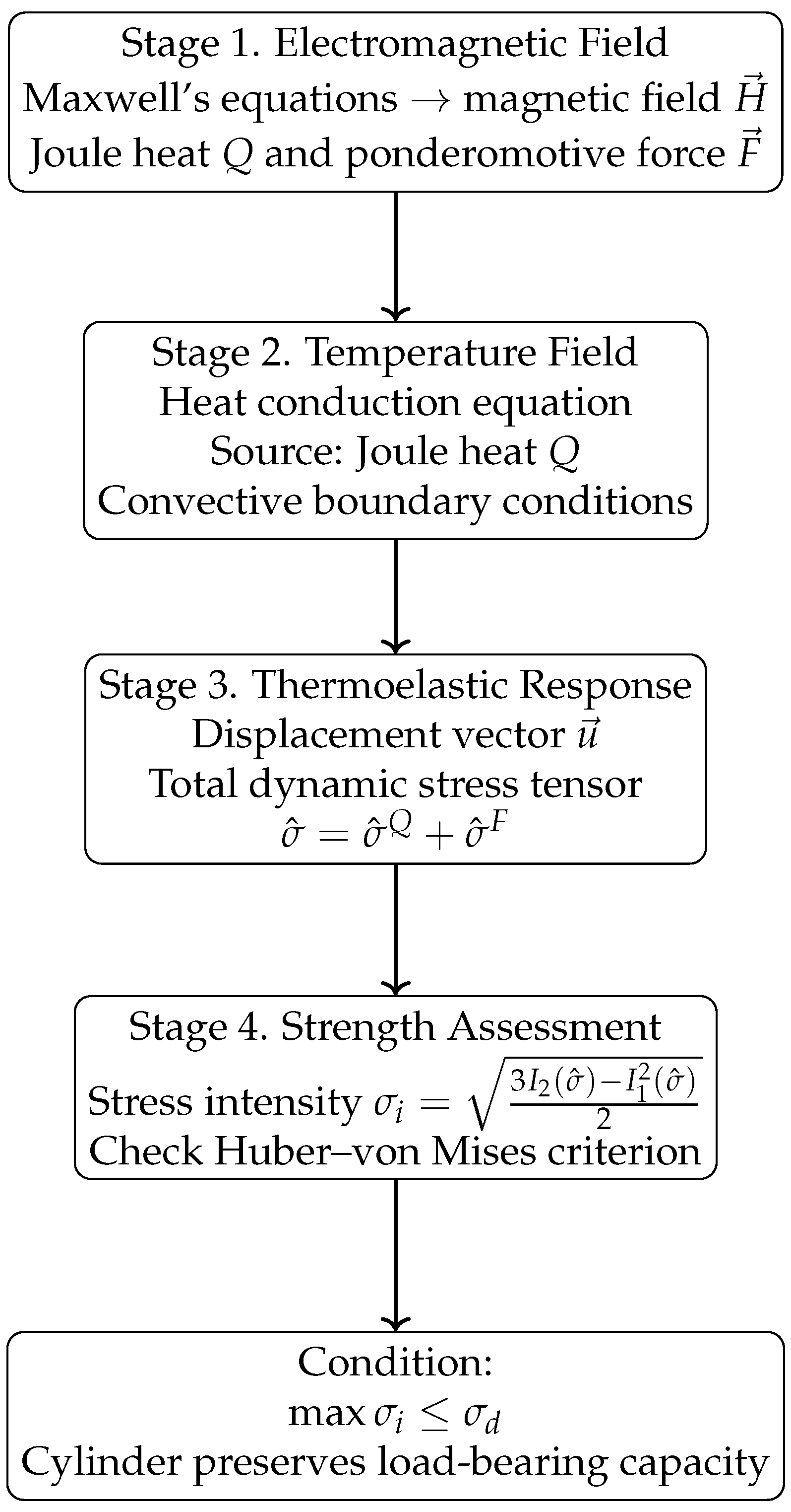
A flow chart of the four-stage physico-mathematical model for determining the thermostressed state of an electroconductive cylinder subjected to an electromagnetic field is presented below (see Figure 1).

At the first stage, the nonstationary EMF is determined from Maxwell’s equations. It is specified by the magnetic field intensity vector $\overrightarrow{H}$ at the surface of the cylinder. At this stage, the resulting Joule heat Q and the ponderomotive force $\overrightarrow{F}$ are also determined.

At the second stage, the nonstationary temperature field T is determined from the heat conduction equation. The volumetric heat source is the Joule heat Q. At the surface of the cylinder, convective heat exchange with the surrounding environment is assumed.

At the third stage, in the absence of surface mechanical loads, the displacement vector $\overrightarrow{u}$ and the total dynamic stress tensor $\widehat{\sigma }={\widehat{\sigma }}^Q+{\widehat{\sigma }}^F$ are determined. They arise due to the Joule heat Q and the ponderomotive force $\overrightarrow{F}$.

At the fourth stage, the load-bearing capacity of the cylinder as a structural element is assessed. To this end, the stress intensity value ${\sigma }_i$ of the total stresses is calculated using the formula [20]

$${\sigma }_i=\sqrt{(3I_2\left(\widehat{\sigma }\right)-I_1^2\left(\widehat{\sigma }\right))/2}.$$

(1)

Here, $I_j\left(\widehat{\sigma }\right)$ denotes the j-invariant of the stress tensor $\widehat{\sigma }$. Subsequently, the stress intensity value ${\sigma }_i$ is compared with the elastic limit ${\sigma }_d$ of the cylinder material. If the Huber–von Mises criterion [20] is satisfied:

$$max{\sigma }_i\le {\sigma }_d,$$

(2)

the cylinder preserves its load-bearing capacity.

3. Dynamic Axisymmetric Plane Problem of Thermomechanics for a Solid Electroconductive Cylinder

3.1. Determination of the EMF

The action of the EMF on the cylinder is determined by the axial component $H_z(r,t)$ of the magnetic field intensity vector $\overrightarrow{H}$ at its outer surface $r=R$:

$$H_z\left(R,t\right)=H_z^{+}\left(t\right).$$

(3)

Here, $H_z^{+}\left(t\right)$ is a prescribed function of time t.

The function $H_z(r,t)$ is determined from the following equation:

$${\displaystyle \frac{{\partial }^2{H}_z}{\partial r^2}}+{\displaystyle \frac{1}{r}}{\displaystyle \frac{\partial H_z}{\partial r}}-\sigma \mu {\displaystyle \frac{\partial H_z}{\partial t}}=0.$$

(4)

Here, $\sigma$ and $\mu$ are the coefficient of electrical conductivity and the magnetic permeability of the electroconductive cylinder material, respectively. Equation (4) is solved subject to the boundary condition (3) at $r=R$, the axisymmetric condition of EMF at the cylinder axis $r=0$:

$${\displaystyle \frac{\partial H_z\left(0,t\right)}{\partial r}}=0$$

(5)

and the zero initial condition:

$$H_z\left(r,0\right)=0.$$

(6)

The specific densities of the Joule heat $Q(r,t)$ and the radial component $F_r(r,t)$ of the ponderomotive force vector $\overrightarrow{F}=\{F_r;0;0\}$ are calculated using:

$$Q={\displaystyle \frac{1}{\sigma }}{\left({\displaystyle \frac{\partial H_z}{\partial r}}\right)}^2,$$

(7)

$$F_r=-\mu H_z{\displaystyle \frac{\partial H_z}{\partial r}}.$$

(8)

3.2. Determination of the Temperature Field

The temperature field $T(r,t)$ in the considered cylinder, generated by the Joule heat $Q(r,t)$, is determined from the heat conduction equation:

$${\displaystyle \frac{{\partial }^{2}T}{\partial r^2}}+{\displaystyle \frac{1}{r}}{\displaystyle \frac{\partial T}{\partial r}}-{\displaystyle \frac{1}{\kappa }}{\displaystyle \frac{\partial T}{\partial t}}=-{\displaystyle \frac{Q}{\lambda }}.$$

(9)

Here, $\kappa$ and $\lambda$ are the coefficients of thermal diffusivity and thermal conductivity of the electroconductive cylinder material, respectively.

Equation (9) is solved under the boundary condition of convective heat exchange at $r=R$ and the symmetry condition of the temperature field at the axis $r=0$:

$${\displaystyle \frac{\partial T\left(0,t\right)}{\partial r}}=0,$$

(10)

along with the zero initial condition:

$$T\left(r,0\right)=0.$$

(11)

3.3. Determination of the Thermostressed State

The radial component $u_r(r,t)$ of the displacement vector $\overrightarrow{u}=\{u_r;0;0\}$, caused by the temperature $T(r,t)$ and the ponderomotive force $F_r(r,t)$, is obtained for the considered cylinder from the following equation

$${\displaystyle \frac{{\partial }^2{u}_r}{\partial r^2}}+{\displaystyle \frac{1}{r}}{\displaystyle \frac{\partial u_r}{\partial r}}-{\displaystyle \frac{1}{r^2}}{u}_r-{\displaystyle \frac{1}{c_1^2}}{\displaystyle \frac{{\partial }^2{u}_r}{\partial t^2}}=\alpha {\displaystyle \frac{1+\nu }{1-\nu }}{\displaystyle \frac{\partial T}{\partial r}}-{\displaystyle \frac{\left(1+\nu \right)\left(1-2\nu \right)}{E\left(1-\nu \right)}}{F}_r.$$

(12)

Here, $c_1={\left({\displaystyle \frac{E(1-\nu )}{\rho (1+\nu )(1-2\nu )}}\right)}^{{\displaystyle \frac{1}{2}}}$ is the velocity of the longitudinal elastic wave in the cylinder material, E is Young’s modulus, $\nu$ is Poisson’s ratio, $\rho$ is the material density, and $\alpha$ is the coefficient of linear thermal expansion.

Equation (12) is solved subject to the traction-free boundary condition at the surface $r=R$:

$$\left(1-\nu \right){\displaystyle \frac{\partial u_r}{\partial r}}+\nu {\displaystyle \frac{1}{r}}{u}_r-\alpha \left(1+\nu \right)T=0$$

(13)

and is subject to the condition of $u_r$ radial displacement axisymmetry at the cylinder axis $r=0$:

$${\displaystyle \frac{\partial u_r\left(0,t\right)}{\partial r}}=0$$

(14)

and the zero initial conditions:

$$u_r\left(r,0\right)=0,{\displaystyle \frac{\partial u_r\left(r,0\right)}{\partial t}}=0.$$

(15)

The components ${\sigma }_{jj}$$(j=r,\phi ,z)$ of the dynamic stress tensor $\widehat{\sigma }$ are calculated based on the previously determined radial displacements $u_r$ and the temperature T using the following expressions [21]:

$${\sigma }_{rr}={\displaystyle \frac{\mathrm{E}}{\left(1+\nu \right)\left(1-2\nu \right)}}\left[\left(1-\nu \right){\displaystyle \frac{\partial u_r}{\partial r}}+\nu {\displaystyle \frac{1}{r}}{u}_r-\alpha \left(1+\nu \right)T\right],$$

(16)

$${\sigma }_{\phi \phi }={\displaystyle \frac{\mathrm{E}}{\left(1+\nu \right)\left(1-2\nu \right)}}\left[\left(1-\nu \right){\displaystyle \frac{u_r}{r}}+\nu {\displaystyle \frac{\partial u_r}{\partial r}}-\alpha \left(1+\nu \right)T\right]$$

(17)

$${\sigma }_{zz}=\nu \left({\sigma }_{rr}+{\sigma }_{\phi \phi }\right)-\alpha ET.$$

(18)

Using the calculated components ${\sigma }_{jj}$$(j=r,\phi ,z)$ of the dynamic stress tensor $\widehat{\sigma }$, the stress intensity values ${\sigma }_i$ are determined according to Formula (1). The load-bearing capacity of the considered cylinder is then assessed using condition (2).

4. Solving Method for the Initial-Boundary Value Problems

An approximation of all determining functions $\Phi (r,t)=\{H_z,T,u_r\}$ with respect to the radial coordinate r is performed using the cubic polynomials [20]:

$$\Phi \left(r,t\right)=\sum _{i=1}^4{a}_{i-1}^{\Phi }\left(t\right)r^{i-1}.$$

(19)

The coefficients $a_{i-1}^{\Phi }\left(t\right)$ of the approximation polynomials (19) are determined using the prescribed boundary values of the functions $\Phi (r,t)$ at the cylinder surface $r=R$, together with their integral characteristics with respect to the radial coordinate r. These characteristics are defined as

$${\Phi }_s\left(t\right)={\displaystyle \frac{s+k}{R^{s+k}}}{\int }_0^R\Phi (r,t)r^{s+k}dr,(s=1,2).$$

(20)

Here, $k=0$ for the functions $H_z\left(r,t\right)$ and $T\left(r,t\right)$, and $k=1$ for the radial displacement $u_r\left(r,t\right)$. Using these relations, the coefficients $a_k\left(t\right)$ for the function $H_z(r,t)$ can be expressed as the linear combination

$$a_k\left(t\right)=a_{k1}{H}_{z1}\left(t\right)+a_{k2}{H}_{z2}\left(t\right)+a_{k3}{H}_z^{+}\left(t\right)$$

(21)

of the integral characteristics $H_{z1}\left(t\right)$, $H_{z2}\left(t\right)$ of the function $H_z(r,t)$, and $H_z^{+}\left(t\right)$ denotes its value at the outer surface of the cylinder $r=R$. Similarly, the coefficients $b_k\left(t\right)$ for the function $T(r,t)$ are represented as

$$b_k\left(t\right)=b_{k1}{T}_1\left(t\right)+b_{k2}{T}_2\left(t\right),$$

(22)

where $T_1\left(t\right)$ and $T_2\left(t\right)$ are the integral characteristics of the temperature distribution $T(r,t)$, obtained under the condition of thermal insulation of the cylinder surface. The coefficients $c_k\left(t\right)$ corresponding to the radial displacement $u_r\left(r,t\right)$ take the form

$$c_k\left(t\right)=c_{k1}{u}_{r1}\left(t\right)+c_{k2}{u}_{r2}\left(t\right)+c_{k3}T(R,t),$$

(23)

where $u_{r1}\left(t\right)$ and $u_{r2}\left(t\right)$ are the integral characteristics of the radial displacements $u_r\left(r,t\right)$, and $T(r,t)$ is the temperature at the cylinder surface.

The numerical values of the coefficients $a_{k1}$, $a_{k2}$, $a_{k3}$, $b_{k1}$, $b_{k2}$, $c_{k1}$, $c_{k2}$, and $c_{k3}$ depend on the cylinder radius R and on the physical and mechanical properties of the material.

To determine the integral characteristics ${\Phi }_s\left(t\right)$ of the governing functions $\Phi (r,t)$, the original Equations (4), (9) and (12) are integrated with respect to the radial coordinate according to relation (20). Substituting the approximations (19) and the representations (21)–(23) into these integrals yields a system of equations for the integral characteristics of the magnetic field $H_z(r,t)$:

$$\left\{\begin{array}{c}{\displaystyle \frac{d{H}_{z1}\left(t\right)}{dt}}-d_1{H}_{z1}\left(t\right)-d_2{H}_{z2}\left(t\right)=d_3{H}_z^{+}\left(t\right)\\ {\displaystyle \frac{d{H}_{z2}\left(t\right)}{dt}}-d_4{H}_{z1}\left(t\right)-d_6{H}_{z2}\left(t\right)=d_7{H}_z^{+}\left(t\right)\end{array}\right.$$

(24)

and the system of equations for integral characteristics $T_s\left(t\right)$ of functions $T(r,t)$:

$$\left\{\begin{array}{c}{\displaystyle \frac{d{T}_1\left(t\right)}{dt}}-d_1^T{T}_1\left(t\right)-d_2^T{T}_2\left(t\right)=Q_1\left(t\right)\\ {\displaystyle \frac{d{T}_2\left(t\right)}{dt}}-d_3^T{T}_1\left(t\right)-d_4^T{T}_2\left(t\right)=Q_2\left(t\right)\end{array}\right..$$

(25)

Here, $Q_j\left(t\right)={\displaystyle \frac{\kappa }{\lambda }}{\int }_0^{R}Q\left(r,t\right)r^{j}dr$, $j=1,2$ are the integral characteristics of Joule heat sources.

The system of equations for the integral characteristics of radial displacements has the form

$$\left\{\begin{array}{c}{\displaystyle \frac{d{u}_{r1}\left(t\right)}{dt}}-d_1^u{u}_{r1}\left(t\right)-d_2^u{u}_{r2}\left(t\right)=W_1\left(t\right)\\ {\displaystyle \frac{d{u}_{r2}\left(t\right)}{dt}}-d_3^u{u}_{r1}\left(t\right)-d_4^u{u}_{r2}\left(t\right)=W_2\left(t\right)\end{array}.\right.$$

(26)

Here, $W_1\left(t\right),W_2\left(t\right)$ are the integral characteristics of the expressions on the right side of Equation (12) for radial displacements $u_r\left(r,t\right)$.

Accordingly, the numerical values of the coefficients $d_1÷d_7$, $d_1^T÷d_4^T$, and $d_1^u÷d_4^u$ are determined by the radius R of the cylinder and the physical and mechanical characteristics of its material.

To solve systems (24)–(26), the integral Laplace transform with respect to time t is applied to the integral characteristics $H_{zs}(t)$, $T_s\left(t\right)$, and $u_{rs}\left(t\right)$, assuming zero initial conditions. After performing the transformation and using the decomposition theorem together with the convolution theorem, the integral characteristics $H_{zs}\left(t\right)$, $T_s\left(t\right)$, and $u_{rs}\left(t\right)$ are obtained in the form

$$H_{zs}\left(t\right)=\sum _{k=1}^2{\int }_0^t{A}_s\left(k\right)H_z^{+}\left(\tau \right)e^{p_k\left(t-\tau \right)}d\tau ,s=1,2.$$

(27)

$$T_s\left(t\right)=\sum _{m=1}^2{\int }_0^t\left[B_{s1}\left(m\right)Q_1\left(\tau \right)+B_{s2}\left(m\right)Q_2\left(\tau \right)\right]e^{p_m\left(t-\tau \right)}d\tau ,s=1,2.$$

(28)

$$u_{rs}\left(t\right)=\sum _{n=1}^2{\int }_0^t\left[D_{s1}\left(n\right)W_1\left(\tau \right)+D_{s2}\left(n\right)W_2\left(\tau \right)\right]e^{p_n\left(t-\tau \right)}d\tau ,s=1,2.$$

(29)

Here, $p_k$, $p_m$, and $p_n$ denote the roots of the characteristic equations for systems (24)–(26). The expressions $A_s\left(k\right)$, $B_{s1}\left(m\right)$, $B_{s2}\left(m\right)$, $D_{s1}\left(n\right)$, and $D_{s2}\left(n\right)$ correspond to homogeneous solutions of these systems and are determined by the values of the roots $p_k,p_m$, and $p_n$ of the respective characteristic equations.

Using the obtained expressions (27) for the integral characteristics $H_{2s}\left(t\right)$, together with relations (21) and (19), the expression for the function $H_z(r,t)$ can be determined. Furthermore, employing Formulas (7) and (8), the corresponding expressions for the Joule heat $Q\left(r,t\right)$ and ponderomotive force $F_r(r,t)$ are derived.

5. Numerical Analysis of the Thermostressed State of an Electroconductive Cylinder Under Amplitude-Modulated Radio Impulse Excitation

The calculations were performed for a solid non-ferromagnetic cylinder with a radius $R=0.01\mathrm{m}$, made of AISI 321 steel (0.12% C, 18% Cr, 10% Ni, 1% Ti), which is commonly used in the oil refining industry, mechanical engineering, cryogenic equipment, food industry machinery, and other industrial applications [22,23]. The cylinder is subjected to the action of AMRI generated by high-frequency electromagnetic oscillation sources.

The AMRI action is described mathematically by the expression:

$$H_z^{+}\left(t\right)=k{H}_0\left(\exp \left(-{\beta }_{1}t\right)-\exp \left(-{\beta }_{2}t\right)\right)\cos \omega t,$$

(30)

which characterises the time variation of the axial component $H_z(r,t)$ of the magnetic field intensity vector $\overrightarrow{H}$ at the surface $r=R$ of the cylinder [9].

The calculations were carried out for the following parameters: AMRI duration $t_i={10}^{-4}\mathrm{s}$ and carrier frequency $\omega =6.28·{10}^5{\mathrm{s}}^{-1}$ of the sinusoidal electromagnetic oscillations. This ensures that 10 oscillation periods are contained within the impulse duration $t_i$. The parameters ${\beta }_1$, ${\beta }_2$, characterizing the rise and fall times of the modulating envelope $\phi \left(t\right)=\exp (-{\beta }_{1}t)-\exp (-{\beta }_{2}t)$, which modulates the carrier sinusoidal electromagnetic oscillations, were set to: ${\beta }_1=\mathrm{69,000}$, ${\beta }_2=2{\beta }_1$.

Substituting expression (30) for the function $H_z^{+}\left(t\right)$ into the corresponding relations derived using the proposed methodology, we obtain the expressions for the axial component $H_z(r,t)$ of the magnetic field intensity vector $\overrightarrow{H}$, the specific density of the Joule heat Q, the radial component $F_r$ of the ponderomotive force vector $\overrightarrow{F}$, the temperature T, and the components ${\sigma }_{jj}$ ($j=r,\phi ,z$) of the dynamic stress tensor $\widehat{\sigma }$ in the cylinder.

In Figure 2, Figure 3, Figure 4, Figure 5, Figure 6 and Figure 7, all the studied quantities are related to the quantity $H_0^2$. Note that below, when discussing these quantities, their relation to the quantity $H_0^2$ is omitted for simplicity.

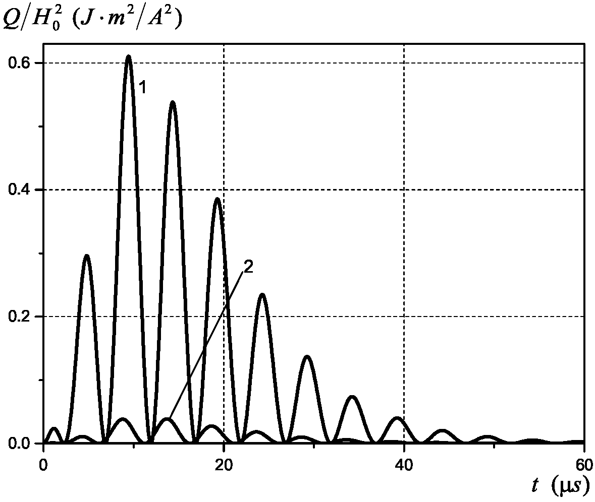
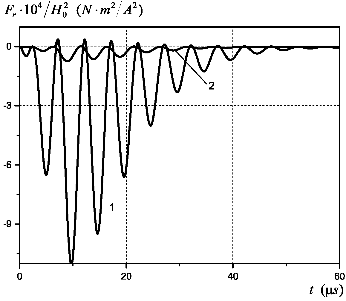
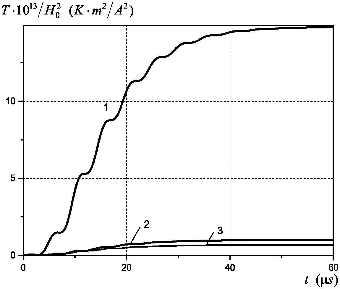
The results of the calculations for the Joule heat Q, the radial component $F_r$ of the ponderomotive force vector $\overrightarrow{F}$, and the temperature T are presented in Figure 2, Figure 3 and Figure 4. Curves 1 and 2 in Figure 2 and Figure 3 correspond to the values of Q and $F_r$ at $r=R$ and $r=0.5R$. Curves 1–3 in Figure 4 correspond to the values of temperature T at $r=R$, $r=0.75R$, and $r=0.5R$.

Analyzing the dependences shown in Figure 2 and Figure 3, it was found that the Joule heat and ponderomotive force consist of modulated thermal and force pulses, the effective action of which occurs over a time of approximately $t=0.3t_i$. From Figure 4, it is obtained that the temperature of the cylinder under consideration reaches maximum values at a time of approximately $t=0.5t_i$. Its distribution over the radius of the cylinder for the selected AMRI parameters has a near-surface character.

To quantitatively assess the contributions of the two physical factors—the Joule heat Q and the ponderomotive force $\overrightarrow{F}$—to the thermostressed state of the solid cylinder, the stress components ${\sigma }_{jj}$ ($j=r,\phi ,z$) of the dynamic stress tensor $\widehat{\sigma }$ are expressed as the sum of two addends:

$${\sigma }_{jj}={\sigma }_{jj}^Q+{\sigma }_{jj}^F.$$

Here ${\sigma }_{jj}^Q$ are the components due to Joule heat, and ${\sigma }_{jj}^F$ is due to the action of the ponderomotive force.

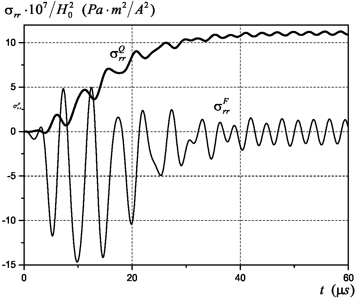
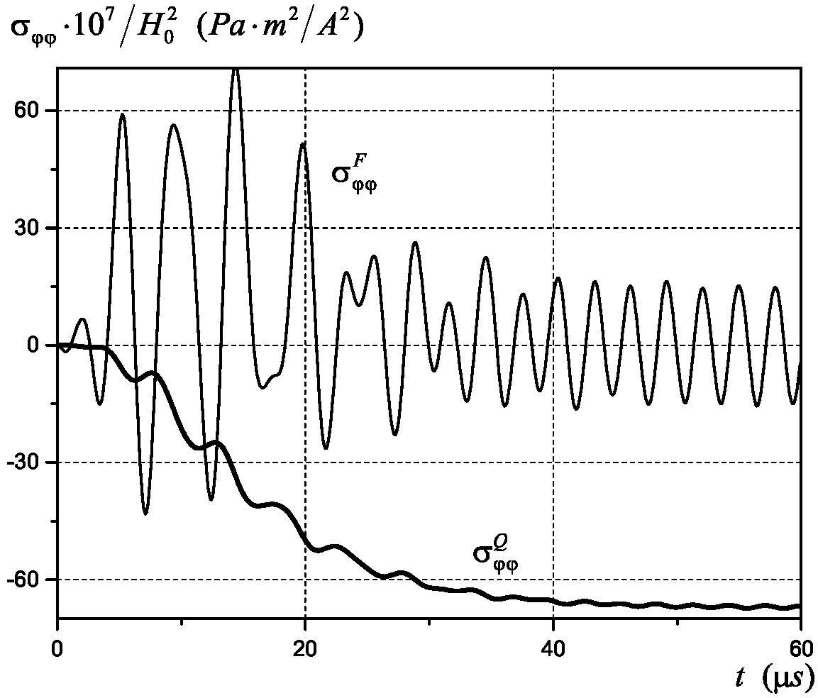
Figure 5 and Figure 6 present the time evolution of the two addends ${\sigma }_{rr}^Q$ and ${\sigma }_{rr}^F$ of the radial stresses ${\sigma }_{rr}$ and the two addends ${\sigma }_{\phi \phi }^Q$ and ${\sigma }_{\phi \phi }^F$ of the circumferential stresses ${\sigma }_{\phi \phi }$ in the cylinder.

In Figure 5, the radial stress addends ${\sigma }_{rr}^Q$ at $r=0.75R$ and ${\sigma }_{rr}^F$ at $r=0.5R$ are shown at positions where their absolute values are maximal. In Figure 6, the circumferential stress addends ${\sigma }_{\phi \phi }^F$ and ${\sigma }_{\phi \phi }^Q$ are evaluated at $r=R$, where their magnitudes are also the highest. The axial stress component ${\sigma }_{zz}$ is determined using the known values of radial ${\sigma }_{rr}$ and circumferential ${\sigma }_{\phi \phi }$ stress components and temperature T according to Formula (18).

Based on the dependencies shown in Figure 5, it is obtained that the effective action of the components ${\sigma }_{rr}^F$ of radial stresses ${\sigma }_{rr}$ occurs at times $t\le 0.25t_i$, and the effective action of the components ${\sigma }_{rr}^Q$ of radial stresses ${\sigma }_{rr}$ occurs at times $t\ge 0.25t_i$. The maximum values of the component ${\sigma }_{rr}^F$, which has a compressive oscillating character, and the same values of the component ${\sigma }_{rr}^Q$, which has a tensile character, are approximately equal to each other in absolute value.

Based on the dependencies shown in Figure 6, it was found that the component ${\sigma }_{\phi \phi }^F$ of the circumferential stresses ${\sigma }_{\phi \phi }$, which has a tensile oscillating character at times $t\le 0.25t_i$ and the component of the circumferential stresses ${\sigma }_{\phi \phi }^Q$, which has a compressive character during time $t_i$ of the duration of the AMRI, are approximately equal in absolute value to each other. This indicates an equivalent contribution of Joule heat and ponderomotive force to the stressed state of the cylinder. It was established that the maximum values of the components of the circumferential stresses are approximately five times greater in absolute value than the corresponding components of the radial stresses.

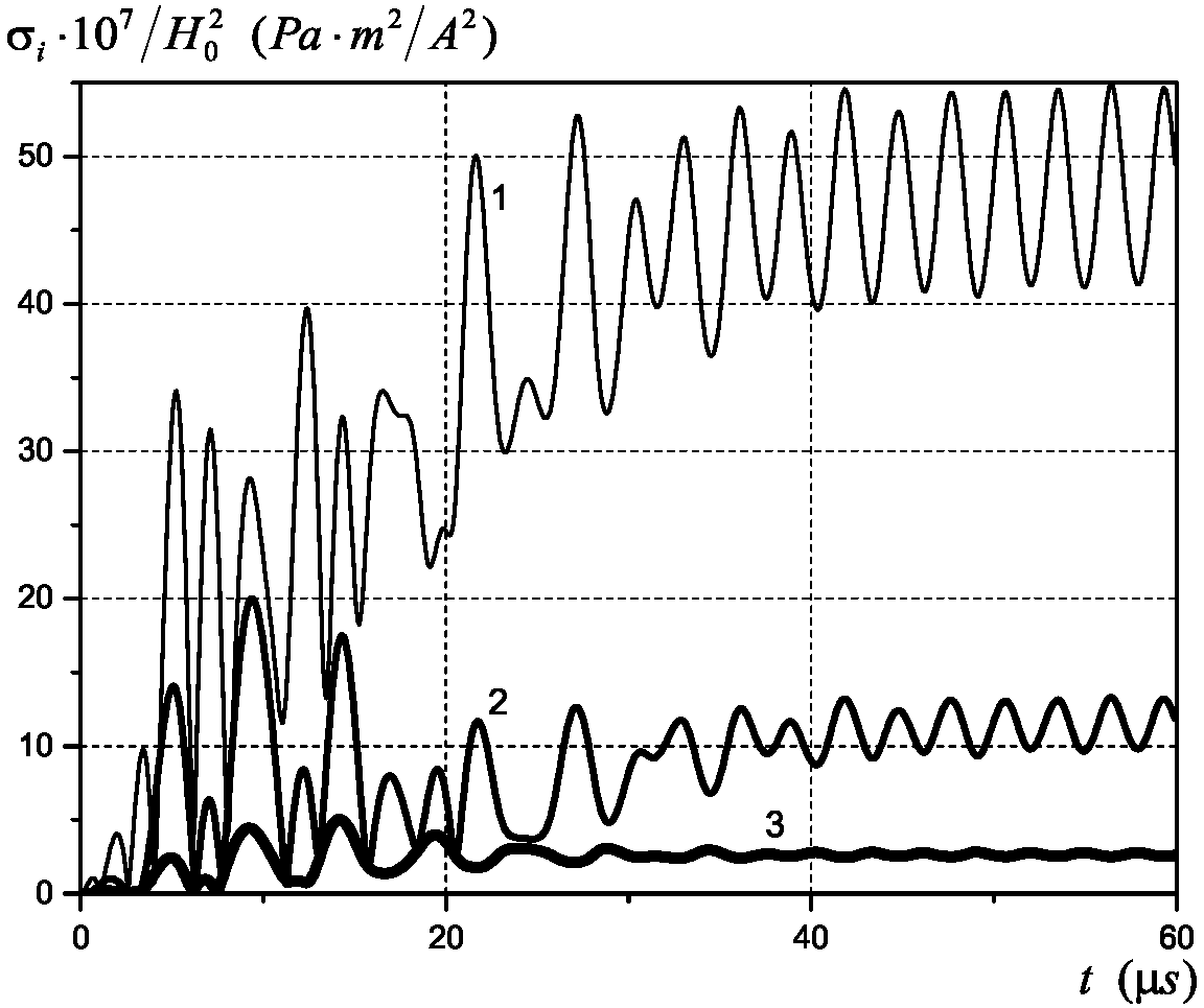
Figure 7 illustrates the time evolution of the value of the total stress intensities ${\sigma }_i$ at $r=R$, $r=0.75R$, and $r=0.5R$ (curves 1–3).

It is obtained that the maximum values of the total stress intensities in the cylinder under consideration are reached on its surface and are approximately 10 times greater than the stresses at $r=0.5R$.

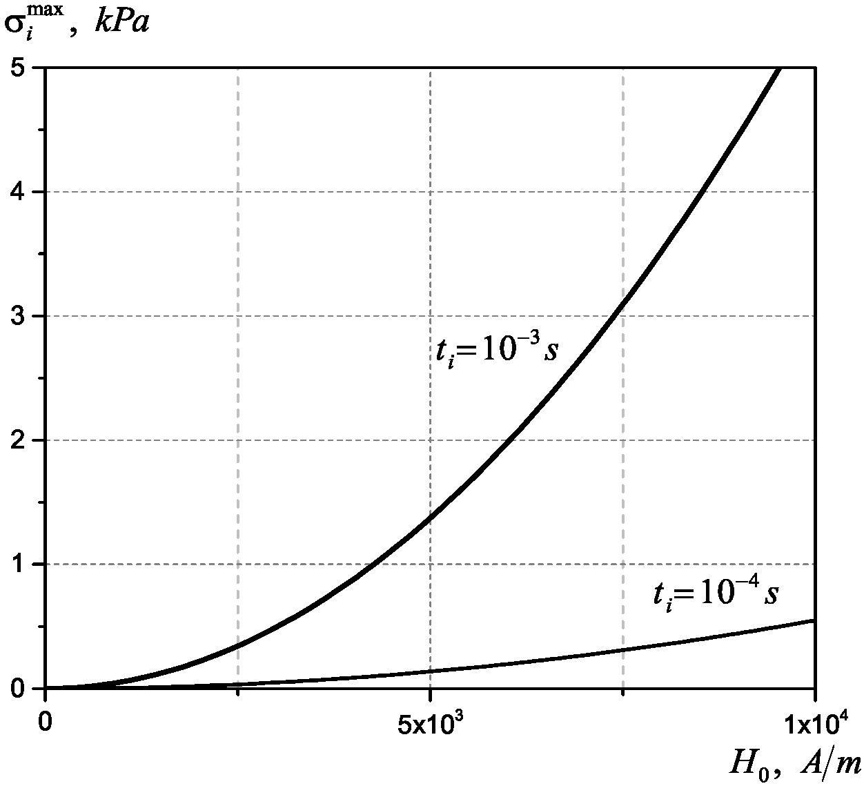
The dependence of the maximum total stress intensity values ${\sigma }_i^{max}$ in the solid electroconductive cylinder on the amplitude $H_0$ of the magnetic field intensity is shown in Figure 8. Thin lines correspond to the AMRI duration $t_i={10}^{-4}$ s, and thick lines correspond to the AMRI duration $t_i={10}^{-3}$ s. For the duration of $t_i={10}^{-4}$ s, the carrier frequency of sinusoidal electromagnetic oscillations is $\omega =6.28·{10}^5 {\mathrm{s}}^{-1}$, and for $t_i={10}^{-3}$ s, the carrier frequency is $\omega =6.28·{10}^4 {\mathrm{s}}^{-1}$. Neither frequency falls within the vicinity of the AMRI resonance frequencies for the considered cylinder.

It was found that at a value of $H_0={10}^4$ A/m during the duration of AMRI $t_i={10}^{-4}$ s, maximum values of the intensity of total stresses are reached, ${\sigma }_i^{max}\approx 0.5$ kPa and ${\sigma }_i^{max}\approx 5$ kPa for $t_i={10}^{-3}$ s. The maximum magnetic field intensity value corresponding to the amplitude $H_0$ of the carrier sinusoidal electromagnetic oscillations with frequency $\omega$, generated by such sources, does not exceed the value of $H_0\le {10}^5\mathrm{A}/\mathrm{m}$ [24]. This means that the pulsed electromagnetic treatment of a solid steel cylinder under the action of the AMRI under consideration is safe from the point of view of the operability of this cylinder as a structural element.

6. Discussion

The Joule heat and the ponderomotive force attain their maximum values at approximately $t\approx 0.1t_i$, whereas the temperature, the components of the dynamic stress tensor, and the total stress intensity attain their maximum values at around $t\approx 0.5t_i$. Both temperature and total stress intensities exhibit maximum values at the cylinder surface and decrease sharply towards its axis.

The influence of the two physical factors—Joule heat and the ponderomotive force—on the stress state of the cylinder is approximately equivalent. This effect is manifested as follows: for time moments $t\le 0.25t_i$, the influence of the ponderomotive force on the magnitudes of the radial and circumferential stresses dominates. The compressive radial stresses ${\sigma }_{rr}^F$ and the tensile circumferential stresses ${\sigma }_{\phi \phi }^F$ are predominant. The tensile radial stresses ${\sigma }_{rr}^Q$ and the compressive circumferential stresses ${\sigma }_{\phi \phi }^Q$ become dominant for $t>0.25t_i$. Throughout the AMRI duration $t_i$, the maximum values of the total circumferential stresses ${\sigma }_{\phi \phi }$ are approximately five to six times greater than the corresponding total radial stresses ${\sigma }_{rr}$.

The maximum values of the total stress intensity ${\sigma }_i^{max}$ under a magnetic field intensity of $H_0\le {10}^4$ A/m and AMRI durations of $t_i={10}^{-4}$ s and $t_i={10}^{-3}$ s are significantly lower than the elastic limit ${\sigma }_d=300$ MPa of the material (steel) of the considered cylinder.

According to the Huber–von Mises criterion, the considered cylinder preserves its load-bearing capacity as a structural element under the specified AMRI parameters. Therefore, AMRIs with such characteristics can be applied for the safe technological impulsed electromagnetic processing of steel cylinders.

Based on the conducted studies, it can be predicted that for the duration of AMRI $t_i\approx 0.4÷0.5$ s and the magnitude of the magnetic field strength $H_0={10}^4$ A/m, the intensity of the total stresses in the steel cylinder under consideration can reach the limit of elastic deformation of its material, as confirmed by experimental studies [22].

7. Conclusions

As a result of the numerical analysis of the thermomechanical behavior of an electroconductive solid cylinder under electromagnetic action in the mode with a pulsed modulating signal, the limiting values of the amplitude–frequency parameters of the electromagnetic field were established at which the considered non-ferromagnetic cylinder retains its load-bearing capacity as a structural element. The new regularities revealed of the thermomechanical behavior of the considered solid non-ferromagnetic cylinder under the action of AMRI form a scientific basis for the selection of rational modes of induction-pulse electromagnetic processing of non-ferromagnetic cylindrical rod-type elements. Future research directions include studying non-ferromagnetic materials under continuous (deep) induction heating and extending the mathematical model to ferromagnetic materials.