Extended State Observer-Assisted Fast Adaptive Extremum-Seeking Searching Interval Type-2 Fuzzy PID Control of Permanent Magnet Synchronous Motors for Speed Ripple Mitigation at Low-Speed Operation

Abstract

Permanent magnet synchronous motors (PMSMs) are utilized in demanding conditions and applications requiring precision and accuracy, such as servo systems. Especially at low speeds, the effects of cogging torque, current measurement and offset errors, improper controller gains, mechanical resonance, and torque fluctuations caused by load torque and flux result in fluctuations at various frequencies in the motor output speed. This study, motivated by two factors, proposes an extended state observer (ESO)-based multivariable fast response extremum-seeking (FESC) interval type-2 fuzzy PID (IT2FPID) controller to improve dynamic response and reduce speed ripple at low speeds in situations where all these negative factors could arise. This approach enables the real-time adaptation of parameters to counteract the decline in controller performance caused by the nonlinear characteristics of PMSMs and parameter fluctuations while also optimizing disturbance rejection in the speed response under varying operating conditions and existing speed ripple. The experimental results from the prototype setup validate that the proposed control mechanism is functional, valid, and precise in diminishing speed ripples during low-speed operations. The simulation and test outcomes of the control scheme show that speed noise at low speeds is reduced from 26% to 3% compared to traditional proportional-integral (PI) controller and supertwisting (STW) sliding mode controller (SMC) responses and that the scheme exhibits a 16–23% reduction in undershoot amplitude and faster recovery in the presence of load torque variations.

1. Introduction

Permanent magnet synchronous motors, known for their superior dynamic response, high power density, outstanding performance, and increased torque density, have been widely employed in electric vehicles, aerospace applications, and various industrial sectors [1,2]. In certain low-speed usage, the gearbox is eliminated from conventional PMSM servo systems to attain greater accuracy. The servo system in question is a direct drive permanent magnet synchronous motor. It offers the following benefits: a small structure, excellent transmission performance, rapid dynamic response, high positional precision, and low distortion [3]. Nevertheless, the absence of a mechanical transmission means that any fluctuations in the speed of the PMSM would immediately impact the load of the direct drive PMSM servo system. This will result in vibrations and pulsation in the load. It is imperative to research methods for reducing speed fluctuations [4,5]. In this kind of system, several factors can lead to speed noise and oscillation: (1) cogging torque, (2) flux-based harmonics, (3) current measurement and offset errors, (4) load disturbance, (5) dead time effect, etc. [6,7]. Torque fluctuations lead to repeated speed oscillations, particularly at low speeds, negatively impacting driver performance [8]. In numerous low-speed implementations, cogging torque is the primary influence compared to other effects. Consequently, numerous studies have investigated the impact of cogging torque on minimizing speed noise during low-speed operations. There are fundamentally two approaches to reducing cogging torque. The first is direct and involves modifications to motor design. However, cost, application difficulty, and complexity can reduce the method’s success rate. The second approach relies on developing motor control strategies [9,10,11]. The second approach is considered a more effective and suitable approach by researchers due to its cost-effectiveness. In this study, control methods are also addressed from the same perspective.

The conventional vector control method commonly employs PI controllers to accurately follow step or ramp input reference signals in motor control. However, these controllers demonstrate inferior performance in the presence of periodic disturbances due to their restricted bandwidth frequency and parameter dependence [12]. Furthermore, the PMSM servo system is characterized by nonlinearity, time variability, and complexity, and it involves inevitable, unmeasured disturbances and parameter variations. Using simple linear control methods [13,14] makes it extremely challenging to achieve suitable performance across the entire operating range [15], especially at low speeds. The sliding mode control method is well known for its ability to maintain its performance in the presence of parameter changes and external disturbances. This ensures faultless tracking performance, regardless of parameter or model uncertainty [16]. It also includes the suppression of aperiodic disturbances [17]. Nonetheless, to guarantee the accuracy of sliding mode control, it is indispensable to select large control gains. However, these large gains have been linked to the well-known chattering phenomenon, which can stimulate high-frequency dynamics [16]. Model Predictive Control (MPC) is a highly researched advanced control methodology in recent years, recognized for producing effective and robust control responses. The core principle of MPC logic is to optimize a cost function based on the error between the setpoint and the feedback value. It is used both independently and in compound controller form in the literature. Some of the recommended MPC controllers for reducing speed fluctuations and improving control performance include FCS-MPC [18], observer-integrated MPC [19,20], duty cycle modification-based MPC [21,22], and continuous-time MPC. Although the MPC system produces a response that improves control performance, it undermines the advantages of the method’s dependence on model and system parameters in control [17]. In addition to these, other methods include backstepping control [23], robust control [24], and intelligent control [25]. However, the disadvantages mentioned above also apply to these methods. The fuzzy logic methodology appears to be an appropriate choice for control systems characterized by significant uncertainty and unexpected events, as it does not depend on a precise mathematical model [26]. Nevertheless, conventional type-1 fuzzy sets may inadequately handle the uncertainty inherent in nonlinear systems due to the ambiguity of fuzzy rules and membership functions [27]. Moreover, fixing these imperfections through trial and error is costly and may be difficult to execute in real time. To eliminate or mitigate these issues arising from type-1-based fuzzy logic controllers, a type-2 fuzzy logic controller has been developed for systems with uncertainty and nonlinearity. This method has better stability and flexibility. This method is also more suitable in cases where defining a membership function in fuzzy sets is difficult [28,29].

The second part of the scientific literature concentrates on mitigating speed disturbances caused by external factors. The most recognized approaches pertaining to this issue involve resonant and repetitive control, both of which fall under the category of internal model-based procedures. The repetitive regulator operates within a periodic signal framework, whereas the resonant controller exhibits infinite gain at the interference frequency [30]. The resonant regulator, when utilized in conjunction with a PI controller, efficiently minimizes ripples at the resonant frequency [31,32]. Repetitive controllers can be regarded as multi-resonant controllers configured in a cascade, which helps reduce rippling at multiple cycle frequencies. Nonetheless, both resonant and repetitive controls are ineffective in mitigating direct current (DC) disturbances. The harmonic injection method [33] is commonly used to eliminate disturbances at a specific frequency by adding a sine wave of that frequency. Nonetheless, these methods require pre-specifying the sine wave’s frequency and amplitude while disregarding other frequency components. One of the most effective methods for mitigating the adverse effects of uncertainties and disturbances arising from unmodeled dynamics and parameter value deviations is to use a controller in conjunction with an ESO [34].

Extremum-seeking control (ESC) is a practical approach to solving real-time optimization problems [35]. ESC can adjust IT2FPID gains by minimizing the squared control error value. To accelerate ESO dynamics and minimize motor speed fluctuations, a proportional–integral-based ESC (PIESC) algorithm is used to achieve faster transient responses, thereby reducing low-speed fluctuations. It yields several main contributions:

(1)

An enhanced speed control technique has been developed that exploits the superior dynamic performance of IT2FPID, eliminates the necessity for motor parameters, and incorporates modifications to control parameters to adapt to variations in operating conditions. This method minimizes response time and mitigates overshoot and undershoot during load torque fluctuations.

(2)

In the external speed loop, the IT2FPID controller functions in conjunction with the ESO to mitigate internal and external disturbances.

(3)

Utilizing a rapid response ESC for controller parameter adaptation and online optimization effectively alleviates the effects of all disturbances, resulting in an integrated resolution to issues.

In the remainder of this article, Section 2 explains the mathematical model of the PMSM and the causes of ripple. Section 3 contains details about the proposed controller components. In Section 4, the experimental setup, simulation results, experimental results, and performance comparisons are included. A conclusion is provided in Section 5.

2. Mathematical Model and Speed Ripple Causes

2.1. Mathematical Model of PMSM

For vector control in PMSMs, a synchronous reference frame is used. In the rotating synchronous reference frame, the generalized equations are organized as follows.

$${\displaystyle \frac{d{i}_d}{dt}}={\displaystyle \frac{1}{L_d}}(u_{ds}-R_s{i}_d+{\omega }_e{L}_q{i}_q)$$

(1)

$${\displaystyle \frac{d{i}_q}{dt}}={\displaystyle \frac{1}{L_q}}(u_{qs}-R_s{i}_q-{\omega }_e{L}_d{i}_d-{\omega }_e{\psi }_m)$$

(2)

In this context, u_ds and u_qs denote the stator axis voltages over the d and q axes, respectively, whereas i_d and i_q correspond to the stator axis currents in the d-q reference frame. The formula ω_e = pω_m depicts the electrical angular speed, with ω_m indicating the mechanical speed and p denoting the number of pole pairs. R_s represents stator resistance.

$${\displaystyle \frac{d{\omega }_e}{dt}}={\displaystyle \frac{1}{J}}(T_e-B{\omega }_e-T_l)$$

(3)

$$T_e={\displaystyle \frac{3}{2}}p\left[{\psi }_f{i}_q+(L_d-L_q)i_d{i}_q\right]$$

(4)

Additionally, T_e is the electrical torque, ψ_f is the permanent magnet flux linkage, J and B stand for the inertia and viscous damping constant of the load, and T_l represents the load torque. L_d = L_q = L. In a nonsalient PMSM, the d-axis inductance is equivalent to the q-axis inductance. As a result, there is no reluctance torque component [36]. The motor torque constant is given by K_t = 3pψ_f/2. The PMSM speed equation is reformulated using constant coefficients and is presented as follows.

$$\begin{array}{l}{\omega }_e=p{\omega }_m\\ {\displaystyle \frac{d{\omega }_e}{dt}}={\displaystyle \frac{1}{J}}({\displaystyle \frac{3}{2}}{p}^2{\psi }_f{i}_q-B{\omega }_e-p{T}_l)\\ =a_0{i}_q-b_0{\omega }_e-c_0{T}_l\end{array}$$

(5)

where a₀ = 1.5p2Ψf/J, b₀ = −B/J, and c₀ = −T_l/J.

2.2. Speed Ripples

The torque ripple of PMSMs can be classified into three primary forms. The initial type originates from the motor’s physical configuration, including cogging torque and flux harmonics. A second category arises from the drive controller, comprising elements such as incorrect current measurement, signal processing lags, and the dead time phenomenon. The torque harmonics created by a PMSM induce speed harmonics of the equivalent order. The electromagnetic torque can be divided into nominal torque, cogging torque, and reluctance torque. The induced harmonic torque is derived using

$$T_{ex}={\displaystyle \frac{3}{2}}p({\psi }_m{i}_q)+{\displaystyle \frac{3}{2}}p({\psi }_{dh}(\theta )i_q-{\psi }_{qh}(\theta )i_d)$$

(6)

2.2.1. Flux Linkage Harmonics

In Equation (6), the initial component on the right side is essential; torque remains constant when i_q is invariant. The subsequent term in the right portion of the equation may induce harmonic parts. These oscillations result from a correlation between the flux harmonic parts ψ_dh and ψ_qh and the spatial current i_s. In the vector control method, ψ_dh provides rotor flux orientation, and ψ_qh = 0 when the flux distribution is ideal. Achieving an optimal sinusoidal flux density distribution is challenging due to production limitations. In a realistic PMSM, ψ_qh contains sixth harmonics.

$${\psi }_{qh}({\theta }_e)={\displaystyle \sum _{n=1}^{\infty }{\psi }_{q6n}}\mathrm{Cos}(6n{\theta }_e)$$

(7)

where θ_e is the rotor electrical angle, n is a positive constant, and ψ_q6n is the amplitude of flux harmonics on the q axis.

2.2.2. Cogging Torque

Cogging torque arises as the permanent magnet approaches or moves away from the stator teeth. The cogging torque can be expressed by a Fourier series as a function of position:

$$T_{cog}({\theta }_m)={\displaystyle \sum _{k=1}^{\infty }{T}_n\mathrm{Sin}(mk\frac{{\theta }_e}{p})}$$

(8)

where T_n denotes the Fourier coefficients, which represent the amplitude of the nth component, and m is the least common multiple between motor slots and poles [37].

2.2.3. DC Offset Fault

The direct current offset in the stator current data also causes vibrating torque. The electromechanical torque can be constructed because of the offset current as follows:

$$T_e=K_t(i_q-\mathsf{\Delta }{i}_q)=T_{em}-\mathsf{\Delta }{T}_m$$

(9)

where Δi_q is the current offset fault component, and ΔT_m is the vibration torque component resulting from the current offset fault.

$$\mathsf{\Delta }{T}_m={\displaystyle \frac{2}{\sqrt{3}}}{K}_t\mathrm{Cos}({\theta }_e)\sqrt{\mathsf{\Delta }{i}_a^2+\mathsf{\Delta }{i}_a\mathsf{\Delta }{i}_b+\mathsf{\Delta }{i}_b^2}$$

(10)

where i_a and i_b represent phase currents.

2.2.4. Current Scaling Fault

The measured motor phase currents are scaled for analog–digital conversion. The current scaling of the measured current is defined as follows:

$$i_{a,b,cs}=I\mathrm{Sin}({\theta }_e\pm \phi )/K_{a,b,c}$$

(11)

where a, b, and c denote motor phases, and K_a,b,c are scaling factors. Current scaling errors can be written as measured phase currents and ideal phase currents.

$$\mathsf{\Delta }{i}_{a,b,cs}=i_{a,b,cs\_AD}-i_{a,b,cs}$$

(12)

where Δi_a,b,cs is the current scaling error, and i_{a,b,cs_AD} represents the measured current. The difference between the currents occurs due to an additional current value. Hence, the ΔT_ms vibration torque component is produced due to the current scaling fault, depending on θ_e, the electrical position [36].

$$\mathsf{\Delta }{T}_{ms}=({\displaystyle \frac{S_a-S_b}{S_a{S}_b}}){\displaystyle \frac{K_{tc}I}{\sqrt{3}}}[\mathrm{Sin}(2{\theta }_e+{\displaystyle \frac{\pi }{3}})+{\displaystyle \frac{1}{2}}]$$

(13)

3. Controller Design

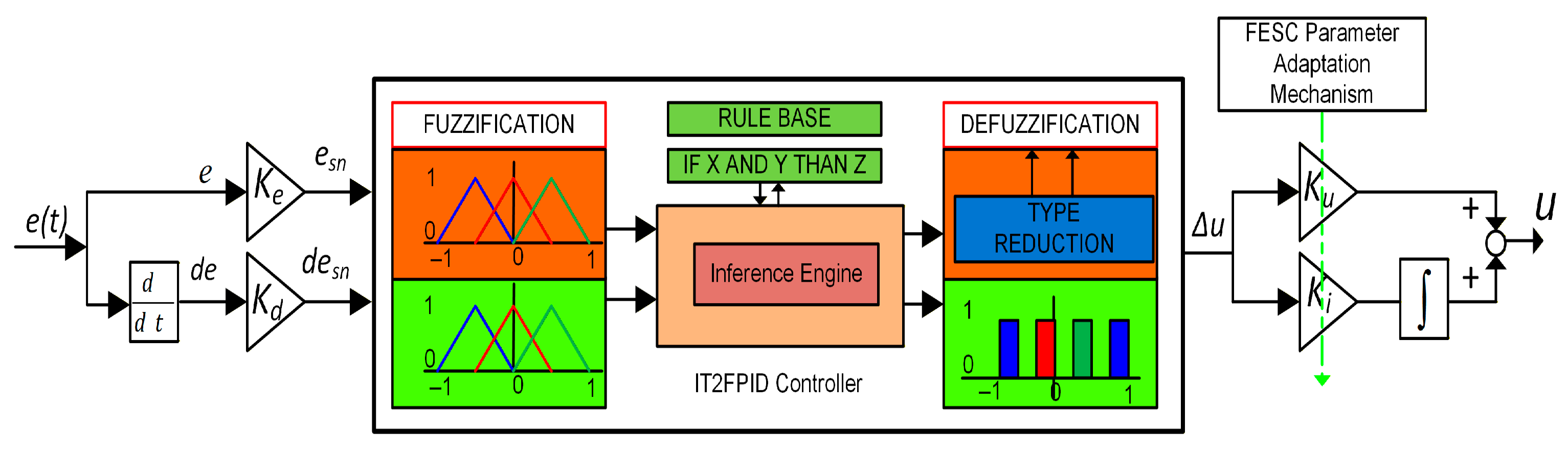
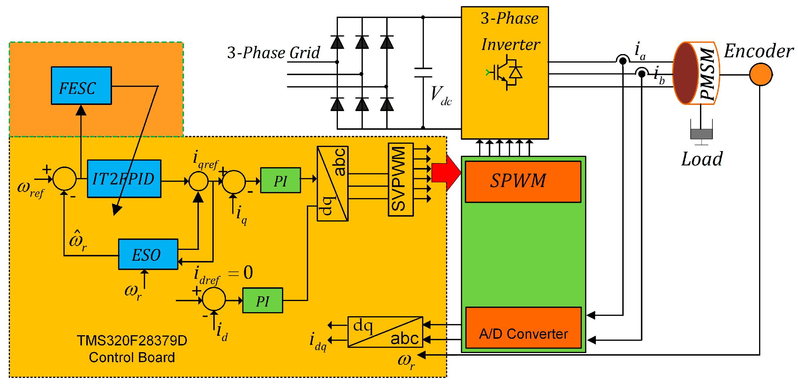
The IT2FPID technique yields a more robust response across various situations, particularly in nonlinear systems such as PMSMs, compared with linear regulators like PI, including parameter changes induced by external and internal factors. The parameters of IT2FPID are updated online using a fast-acting, multivariable extremum-seeking control method. The periodic and non-periodic disturbance effects arising from the mechanical and electrical influences analyzed in the previous section are minimized through online optimization using an extended state observer. IT2FPID, FESC, and the ESO will be clarified in the subsequent sections and are presented in Figure 1 as a block diagram.

3.1. Interval Type-2 Fuzzy PID Controller

Uncertainties are typically characterized as unexpected disturbances, distorted signals, or noise, and different kinds of uncertainty are prevalent in numerous practical applications. The aforementioned uncertainties impact the system’s effectiveness; thus, possessing robust anti-disturbance capacity is of practical significance [38]. Fuzzy logic methods reveal a remarkable capability to cope with multiple uncertainties and disturbances. Across different controller types, type-1 fuzzy PID (T1FPID) control techniques have recently gained attention for multiple reasons. In essence, the fuzzy proportional-integral-derivative (FPID) control approach combines fuzzy proportional-integral (FPI) and proportional-derivative (FPD) controllers, thereby enabling the formation of proportional, integral, and derivative functions for the T1FPID controller, as illustrated in Figure 1. Interval type-2 fuzzy regulators (IT2FLC) provide greater flexibility, offering a wider range of configurations than their type-1 counterparts. This additional flexibility is advantageous in controlling uncertain nonlinear systems [39]. Figure 2 illustrates the structure of the IT2FPID controller.

IT2FLC sets are fuzzy sets, where x signifies the input within the framework of X, and u and z indicate the primary and auxiliary membership levels, respectively.

$$F=\left\{(X,U),{\mu }_F(x,u)\left|\forall x\in X, \right.\forall u\in H_x\subseteq [0,1]\right\}$$

(14)

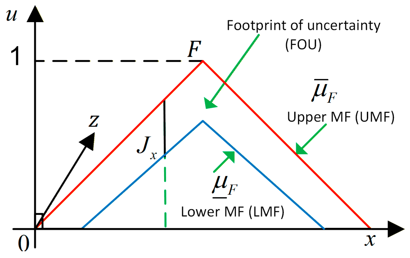
In Figure 3, the region between the upper and lower triangles represents the footprint of indeterminacy (FOI), which consists of two functions of membership (MFs): the lower function of membership (LFM) and the upper function of membership (UFM). FOU denotes the values pertaining to the membership degrees (μ) of the inputs. Consequently, F is also represented as

$$F={\displaystyle \underset{x\in X}{\int }{\displaystyle \underset{u\in J_x}{\int }\frac{{\mu }_F(x,u)}{(x,u)}}},H_x\subseteq [0,1]$$

(15)

The IT2FLC system typically comprises five sections: fuzzification, inference mechanism, rule base, type-reducing, and defuzzification. Initially, the system’s precise input value is processed by the fuzzifier, which converts the discrete value into several IT2FLCs to derive the associated membership degrees. The fuzzy inference mechanism subsequently assesses the firing strength of rules according to the defined standards in its rule base. The inference operation is executed to derive IT2 fuzzy output values, which are subsequently transformed into T1FSs by the system’s type reducer. Ultimately, the T1FSs are defuzzified to produce the system’s final precise output [38]. The domain for the membership functions of the input and output variables e, Δe, and u is scaled to the range of [−1, 1]. N: negative, Z: zero, and P: positive triangular membership functions are used for the inputs, while N: negative, Z: zero, P: positive, B: big, M: medium, and Z: zero singleton membership functions are assigned for the outputs. The rule base comprises the set of rules upon which a particular control system is established. The error e and error derivative Δe are used in the rule base, and fuzzy logic rules are set up for conventional and IT2FLC, respectively, as follows:

$$IF e is X_e^n AND \mathsf{\Delta }e is X_{\mathsf{\Delta }e}^n THEN \mathsf{\Delta }u is Y^n$$

$$\left\{\begin{array}{l}IF e_L is X_{eL}^n AND \mathsf{\Delta }e is X_{\mathsf{\Delta }eL}^n THEN \mathsf{\Delta }u is {\underset{\_}{Y}}^n\\ IF e_U is X_{eU}^n AND \mathsf{\Delta }e is X_{\mathsf{\Delta }eU}^n THEN \mathsf{\Delta }u is {\overline{Y}}^n\end{array}\right.$$

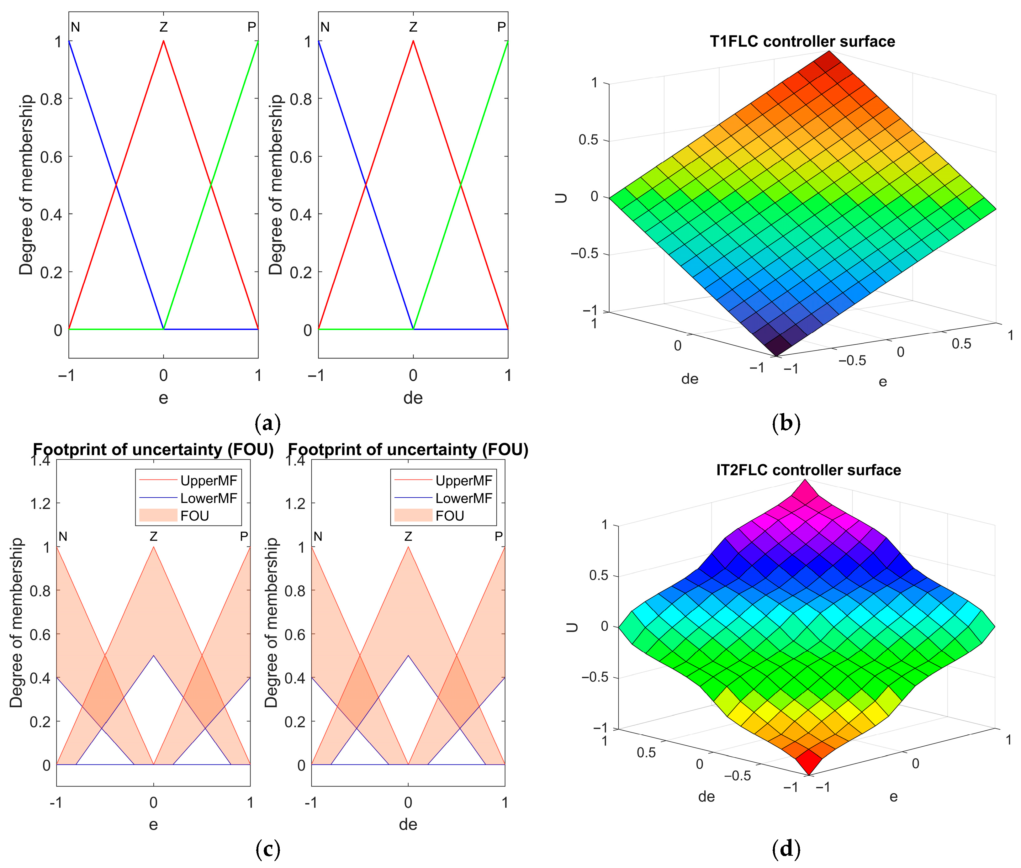
where L is the lower value, U is the upper value, and Y is a singleton fuzzy set. The interval type-2 fuzzy control structure reduces the computational load of type-2 fuzzy regulators. Similarly to the conventional FLC, the inputs are scaled by the K_e and K_d coefficients before being processed in the fuzzification block. IF–THEN rules are executed for both the type-1 fuzzy and type-2 fuzzy algorithms. Figure 4 represents T1FLC and IT2FPID input membership functions and controller output, and error and error derivative surfaces.

The IT2FLC inference method resembles that of type-1 fuzzy logic. The end phase includes type reduction, yielding the type-1 fuzzy set, while a defuzzifier transforms the produced type-1 fuzzy set into a precise value. The implemented IT2FPID method employs product inference and utilizes the center of sets defuzzification procedure. In this research, however, the fuzzy weighted average defuzzification approach is applied.

$$\begin{array}{l}\overline{y}={\displaystyle \frac{{\displaystyle \sum _{i=1}^N{y}^i{f}_u^i}}{{\displaystyle \sum _{i=1}^N{f}_u^i}}}\\ \underset{\_}{y}={\displaystyle \frac{{\displaystyle \sum _{i=1}^N{y}^i{f}_l^i}}{{\displaystyle \sum _{i=1}^N{f}_l^i}}}\\ U=\lambda \underset{\_}{y}+(1-\lambda )\overline{y}\end{array}$$

(16)

where y_i symbolizes the resulting membership functions, and N denotes the overall number of rules. λ signifies a weighting variable for the type-reduced set ([$y, \overline{y}$]), and U indicates the output of IT2FLC. Finally, f_l and f_h are designated as the lower and upper activation functions, respectively. The FLC (fuzzy logic controller) is formed by the combination of outputs from both the FPD and FPI controllers. Therefore, the control output, dependent on the parameters, is expressed as follows. F: The control output u_PID is derived from the proportional, integral, and derivative components, as given by

$$u_{PID}(\tau )\cong C(t)+(K_u{K}_d+K_d{K}_i)e(\tau )+K_e{K}_i{\displaystyle \int e(\tau )}d\tau +K_u{K}_d{\displaystyle \frac{de(\tau )}{d\tau }}$$

(17)

where C(t) is a time-dependent variable that includes FLC rules [40]. Conventional approaches to determining controller parameters rely on professional expertise or computational modeling. To overcome the shortcomings of conventional approaches, the quick response ESC algorithm is employed to adaptively adjust the controller gains K_u, K_i, and K_d. The following section presents an overview of the objective function-based multivariable sliding mode ESC algorithm.

Two input variables are used for PMSM speed control: the speed error e = (ω_ref − ω_actual) and its derivative de = Δe/Δt. Both variables are normalized to the range [−1, 1], and the output variable U, representing the q-axis current reference, is scaled over the same interval. The scaling factors (K_e, K_de, K_u, K_i) are determined through preliminary experimental tests conducted over the system’s operating range. Three triangular membership functions (MFs)—N, Z, and P—are defined for both input variables and the output of the type-1 FLC. The triangular shape is chosen because it is easy to calculate, covers a wide range of possibilities, and works well for real-time use in fast-moving systems like PMSM drives. Adjacent MFs meet at a membership degree of 0.5, which ensures the entire range of possible values is covered, so the rule base can handle every possible input.

The interval type-2 FLC uses the same geometric structure as the T1FLC; however, each MF has both an Upper Membership Function (UMF) and a Lower Membership Function (LMF). The region bounded between them constitutes the Footprint of Uncertainty (FOU). The FOU width was set to ±20% of the corresponding T1 MF. This choice was based on one main factors: known measurement uncertainties related to PMSM parameters, specifically R_s, L_d, and L_q.

The trade-off between robustness to small disturbances and the loss of control precision, which occurs when the FOU is too wide, is shown. Figure 4c shows that the UMF peak is always at 1.0, while the LMF peak is always at 0.5. This configuration provides robustness to measurement noise and load disturbances inherent in PMSM speed control while preserving the necessary sensitivity in the near-zero-error region. Both controllers share an identical rule base consisting of nine rules arranged in a 3 × 3 structure. The rules were formulated heuristically, following the classical design principles of PD-type fuzzy controllers:

In

Table 1. IT2FPID rule base.

e/de	N	Z	P
N	NB	NM	Z
Z	NM	Z	PM
P	Z	PM	PB

, the rule table reflects the following physical reasoning:

e < 0 and de < 0 → speed is below reference and diverging; strong negative control action is required.

e = 0 and de = 0 → steady-state condition; zero control action.

e > 0 and de < 0 → error is decreasing; premature action is unnecessary; moderate response.

Figure 4b illustrates that the T1FLC surface exhibits a nearly smooth, linear characteristic. Conversely, the IT2FLC surface seen in Figure 4d exhibits a clearly nonlinear, saddle-like configuration. The observed discrepancy arises from the FOU’s implementation of differential gain contributions across the input space during type reduction and defuzzification. Consequently, the IT2FLC produces better control measures in low-error regions and more robust responses in high-error regions. This attribute offers improved overshoot suppression and reduced settling time in PMSM speed control.

3.2. Fast Extremum-Seeking Method for Online Parameter Optimization

It is not unusual for controller parameters to lack sufficient robustness to changes in setpoints, internal disturbances, and external disturbances when these factors change instantaneously. In the proposed study, the IT2FPID controller, which exhibits nonlinear behavior, also possesses proportional, integral, and derivative effect parameters. A controller parameter estimation technique utilizing the extremum-searching algorithm is suggested to achieve optimal performance, primarily by reducing overshoot and improving rise time [41]. The aim of the ES algorithm is to identify a PID parameter set that enhances steady-state performance by adjusting the tracking error to the minimum while attenuating vibrations.

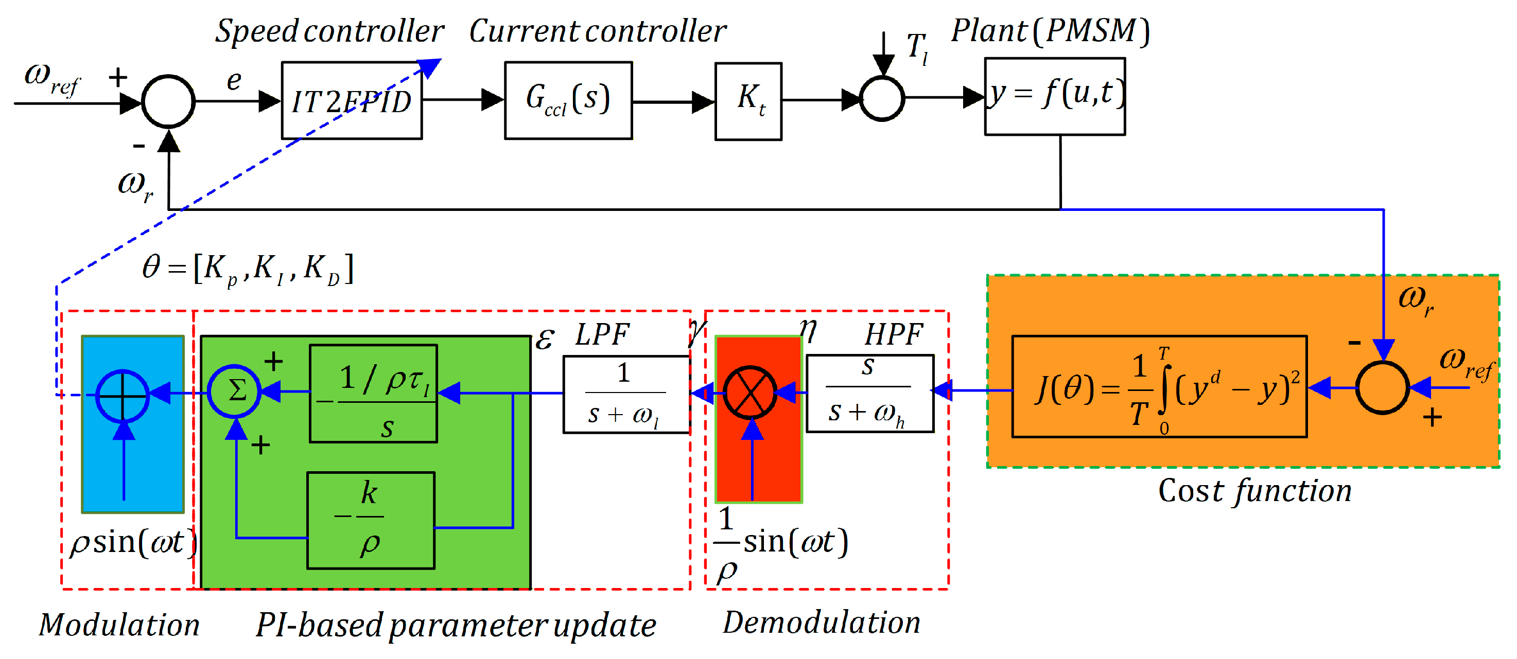
Figure 5 presents a schematic of FESC. Controller parameter estimation does not require prior knowledge of the motor drive system. Speed error information is used as an input to the cost function. In the context of ESC, the high-frequency pulsating signal s = ρSin(ωt) is added to the output signal to enable the search for optimal control parameters. ρ represents the magnitude of the oscillating signal. ω represents the pulsating frequency. The objective of adding this signal is to generate oscillations in the system, assisting the ESC algorithm in determining the gradient or optimization direction. By analyzing the system’s response to these oscillations, the ESC algorithm can modify parameters to identify the optimal point, such as minimal error, maximal efficiency, or minimal speed response ripple.

A high-pass filter (HPF) facilitates the utilization of high-frequency information, whereas the signal demodulation output comprises both DC and high-frequency components.

$$\gamma ={\displaystyle \frac{{\rho }^2}{2}}\eta -{\displaystyle \frac{{\rho }^2}{2}}\eta \mathrm{Sin}(2\omega t)$$

(18)

A low-pass filter is used to determine the DC signal terms, and ε signal information is obtained for PI control input. η represents the HPF output. Assuming the controller parameters are K = [K_p, K_i, K_d] and J, the cost function derived from the error equation can be expressed as follows:

$$J(\theta )={\displaystyle \frac{1}{T}}\underset{t\to \infty }{\lim }{\displaystyle \underset{t}{\overset{t+T}{\int }}({\phi }_1}{e}^2(t)+{\phi }_2{\dot{e}}^2(t))d(t)$$

(19)

where T is referred to as the sampling period, and the positive parameters α₁ and α₂ act as weighting coefficients that account for error and disturbance effects. The proportional–integral ESC approach is designed to enhance the controller’s transient performance. It implies that the equations describing the dynamics of the nonlinear system and the cost function to be minimized are unknown, although measurable.

$$\begin{array}{l}\dot{x}=f(x)+g(x)u, y=h(x)\\ {\dot{K}}_I=-{\displaystyle \frac{1}{\rho {\tau }_I}}\widehat{K}\sin (\omega t)\\ u=-{\displaystyle \frac{k}{\rho }}\widehat{K}\sin (\omega t)+K_I+\rho \sin (\omega t)\end{array}$$

(20)

K represents the actual controller parameters, $\widehat{K}$ is the estimated parameter vector, and $\tilde{K}$ is the parameter estimation error vector. A nonlinear system can be described by the following equation. Accordingly, for u(e,K), the input function can be explained in relation to the output error and the controller settings. The tracking error, e(t), is expressed as

$$e(t)=y_d(t)-y(t)$$

(21)

y_d is the desired output value, and y is the current output value. $K={[K_p{K}_i{K}_d]}^T$ and $\mathsf{\Gamma }(e)={[e(t){\displaystyle \underset{0}{\overset{t}{\int }}{e}_i(\tau )d\tau } d{e}_d/d\tau ]}^T$ can be written as a parameter vector and an error vector.

Stability of Fast Extremum-Seeking Control Methods

In this section, the stability of the fast-acting ESC with proportional–integral action, based on a Lyapunov function, is established. At this point, adaptive gain ESC identifies the most suitable gain values by updating the output of the cost function with the lowest error. Thus, the control input is rearranged in terms of the error and the controller parameters as follows:

$$u(e,K)={\mathsf{\Gamma }}^T(e)K$$

(22)

In this case, the optimal control output u can be explained in terms of the optimal gain vector and gain estimation error.

$$\begin{array}{l}{e}_u={\mathsf{\Gamma }}^T(e)\tilde{K}\\ \tilde{K}=K-\widehat{K}\end{array}$$

(23)

Parameter estimation dynamics are defined as follows:

$$\dot{y}={\mathsf{\Gamma }}^T\widehat{K}+G_{c}e+c^T\dot{\widehat{K}}$$

(24)

where G_c denotes a positive constant, and c denotes the differential equation solution.

$${\dot{c}}^T=-G_c{c}^T+{\mathsf{\Gamma }}^T$$

(25)

The dynamics of estimation error are derived as follows:

$$\dot{y}={\mathsf{\Gamma }}^T\widehat{K}+G_{c}e+c^T\dot{\widehat{K}}$$

(26)

The following parameter update law, as proposed in [42], is considered.

$$\dot{\widehat{K}}=\mathrm{Pr}oj({\displaystyle {\sum }^1(c(e-\widehat{\eta })}-\sigma \widehat{K}),\widehat{K}), \widehat{K}(0)=K^0$$

(27)

The projection algorithm is expressed as

$$\mathrm{Pr}oj(t,u)=\mathsf{\Lambda }(u)(-l\widehat{K}+d(t)), \mathsf{\Lambda }(u)=I$$

(28)

A controller gain estimation stability analysis is carried out according to the Lyapunov function:

$$V={\displaystyle \frac{1}{2}}{\tilde{\eta }}^T\tilde{\eta }+{\displaystyle \frac{1}{2}}{\tilde{K}}^T{\displaystyle \sum \tilde{K}}+{\displaystyle \frac{1}{2}}{K}^{T}K$$

(29)

Differentiating V gives

$$\begin{array}{l}\dot{V}\le -l_a{\tilde{\eta }}^T\tilde{\eta }-l_b{\tilde{K}}^T\tilde{K}-{\displaystyle \frac{1}{2}}{(e-\widehat{\eta })}^T(e-\widehat{\eta })-l_c{K}^T\mathsf{\Lambda }(u)\mathsf{\Gamma }K+l_d{‖d(t)‖}^2\\ \le -l_{V}V+l_d{‖d(t)‖}^2\end{array}$$

(30)

where l_a, l_b, l_c, and l_d are strictly positive constants. There is a time t at which the closed-loop system achieves exponential convergence. For sinusoidal dither signals, convergence necessitates the presence of at least one specific dither frequency for each input. This is equivalent to conventional adaptive control and perturbation-based extremum-seeking control methodologies. The theorem establishes that the response velocity can be modified by augmenting the optimization gain l. An elevation in l leads to a concomitant increase in K. It may be noticed that both requirements are satisfied, yielding negative definite $\dot{V}$(t). Given that $\dot{V}$(t) in the equation is negative definite, and V(t) is positive definite, the average error dynamics exhibit asymptotic stability. All aspects of stability analysis are thoroughly discussed in [35,43].

3.3. Extended State Observer

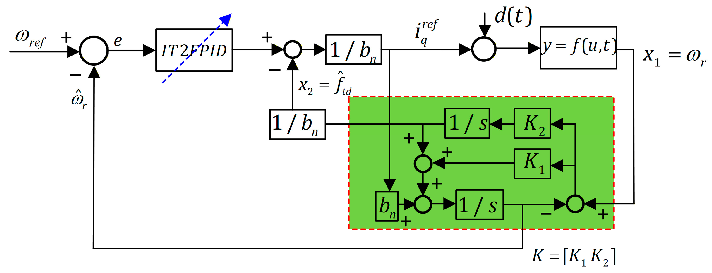
Disturbances in a PMSM are typically induced by causes such as cogging torque, periodic load torque, flux harmonics, stator current sampling inaccuracies, and dead time. The ESO observes the real-time effects of unknown external disturbances and system dynamics and mitigates them through feedback mechanisms. This approach removes the necessity for a disturbance model and is not dependent on the direct measurement of disturbances to evaluate their effects. Nonlinear functions are essential for the ESO to achieve its intended aims, making them a vital element of its design. The extended state observer is formulated for nonlinear systems structured in integral chain form. System dynamics in terms of state variables can be expressed as

$$\begin{array}{l}{\dot{x}}_1=x_2+b_{n}u\\ {\dot{x}}_2={\displaystyle \frac{d}{dt}}f(y,\omega ,t)\end{array}$$

(31)

Based on these dynamics, a linear ESO control algorithm can be formulated as a series of equations.

$$\begin{array}{l}{\widehat{\dot{x}}}_1={\widehat{x}}_2-K_1({\widehat{x}}_1-x)+b_{n}u\\ {\widehat{\dot{x}}}_2=-K_2({\widehat{x}}_1-x)\\ e={\widehat{x}}_1-x\end{array}$$

(32)

$$\begin{array}{l}{\dot{\omega }}_r={\displaystyle \frac{3}{2}}{\displaystyle \frac{p{\psi }_{fn}}{J_n}}{i}_q-{\displaystyle \frac{B_n}{J_n}}{\omega }_r+f_{pd}+f_{ld}\\ =b_n{i}_q\underset{ftd}{\underbrace{-a_n{\omega }_r+f_{pd}+f_{ld}}}\end{array}$$

(33)

where $b_n=3/2(p{\psi }_{fn}/J)$, $a_n=B/J$ and $f_{pd}$ represent motor parameter mismatch, and ${\mathrm{f}}_{\mathrm{l}\mathrm{d}}$ represents load torque changes. In other words, these two disturbance effects can also be referred to as internal and external disturbances.$f_{pd}=-\mathsf{\Delta }J{\omega }_r/J_n-\mathsf{\Delta }B{\omega }_r/J_n+3/2(p\mathsf{\Delta }{\psi }_f{i}_q/J_n)$, $f_{ld}=-p{T}_l/J_n$, $\mathsf{\Delta }J=J-J_n$, $\mathsf{\Delta }B=B-B_n$, and $\mathsf{\Delta }{\psi }_f={\psi }_f-{\psi }_{fn}$ are all disturbances. $J, B$, and ${\psi }_f$ are actual parameter values. An ESO is intended to evaluate the overall disturbance $f_{td}$ instantaneously for the speed regulation loop of the PMSM drive as

$$\begin{array}{l}e={\widehat{\omega }}_r-{\omega }_r\\ \dot{\widehat{\omega }}={\widehat{f}}_{td}-K_{1}e+b_n{i}_q\\ {\dot{\widehat{f}}}_{td}=-K_{2}e\end{array}$$

(34)

The bandwidth of the gains $K_1$ and $K_2$ determines the performance of the ESO.

$$\begin{array}{l}{s}^2+K_{1}s+K_2={(s+{\omega }_0)}^2\\ K_1=2{\omega }_0, K_2={\omega }_0^2\end{array}$$

(35)

For ${\omega }_0$, the bandwidth of the ESO is expressed in second-order control dynamics as above. Figure 6 shows the structure of the ESO, which reacts to variations in error and total disturbance.

3.4. Parameter Adjusting Procedures

In the adjustment procedure of PI controllers, nonlinear effects are generally disregarded, and tuning is conducted according to the criteria established for electric drives. To enhance performance in the cascade control system, the inner loop controller’s response time must be minimized. The primary aim of the outer loop is to guarantee appropriate regulation and stability. The inner loop (current loop) is set up using the modulus optimum approach for rapid response and simplicity, whilst the outer loop (speed loop) is tuned using the symmetric optimum method to enhance system performance with respect to disturbance signals. Modulus optimum and symmetric optimum procedures are two interconnected methodologies used to construct optimal linear control systems in the frequency domain [44].

Table 2. A comparison of controllers’ experimental performance.

Controller	Current Control Loop	Speed Control Loop
PI	$\begin{array}{l}{T}_n=T_1={\displaystyle \frac{L}{R}}, K_1={\displaystyle \frac{1}{R}}, \\ T_i=2K_1{T}_{tot}, \\ K_p={\displaystyle \frac{T_n}{T_i}}, K_i={\displaystyle \frac{1}{T_i}}\\ T_n=2.76 \mathrm{ms}, \\ K_1=0.42, T_{tot}=75 \mathrm{us}, \\ K_p=43, K_i=\mathrm{15,873}\end{array}$	$\begin{array}{l}{T}_n=4T_{tot},T_i=8{\displaystyle \frac{T_{tot}^2}{T_{\tau }}},\\ K_p={\displaystyle \frac{T_n}{T_i}},K_i={\displaystyle \frac{1}{T_i}}\\ T_n=120 \mathrm{us}, T_i=3.7 \mathrm{ms},\\ K_p=0.032, K_i=270\end{array}$
STW-SMC	$\begin{array}{l}u(t)=-k_1\sqrt{\left|s(t)\right|}sign(s(t))+v(t), \\ \dot{v}(t)=-k_{2}sign(s(t))\\ k_1=\sqrt{{\displaystyle \frac{2}{k_2}}}, k_2>0, k_1=4.47, k_2=0.1\end{array}$
FESC-IT2FPID-ESO	$\begin{array}{l}{s}^2+K_{1}s+K_2={(s+{\omega }_0)}^2\\ K_1=2{\omega }_0, K_2={\omega }_0^2, {\omega }_s=0.01{\omega }_c, {\omega }_c=0.1{\omega }_{pwm}\\ {\omega }_c=1000 \mathrm{rad}/\mathrm{s}, {\omega }_s=10 \mathrm{rad}/\mathrm{s}, K_1=20{,}_{K2}=100\\ f_{esc}=150 \mathrm{Hz}, K_{esc}=0.001,\tau =0.02\end{array}$

presents numerical values for the parameter tuning methods of the speed and current controllers. Since the current controller parameters are the same for the PI, STW sliding mode controller, and FESC-IT2FPID-ESO, the parameters are only provided for the PI controller. Here, K_p, K_i, τ, T_tot, and T_i are the proportional gain, integral gain, system time constant, total time delay, and integral time constant, respectively. The overall time delay is the sum of the PWM, detection, and control loop scanning cycle times. Besides this, STW sliding mode controller speed loop parameter tuning can be performed using geometric and finite-time convergence techniques. In this study, the second technique is preferred.

4. Experimental Hardware and Results

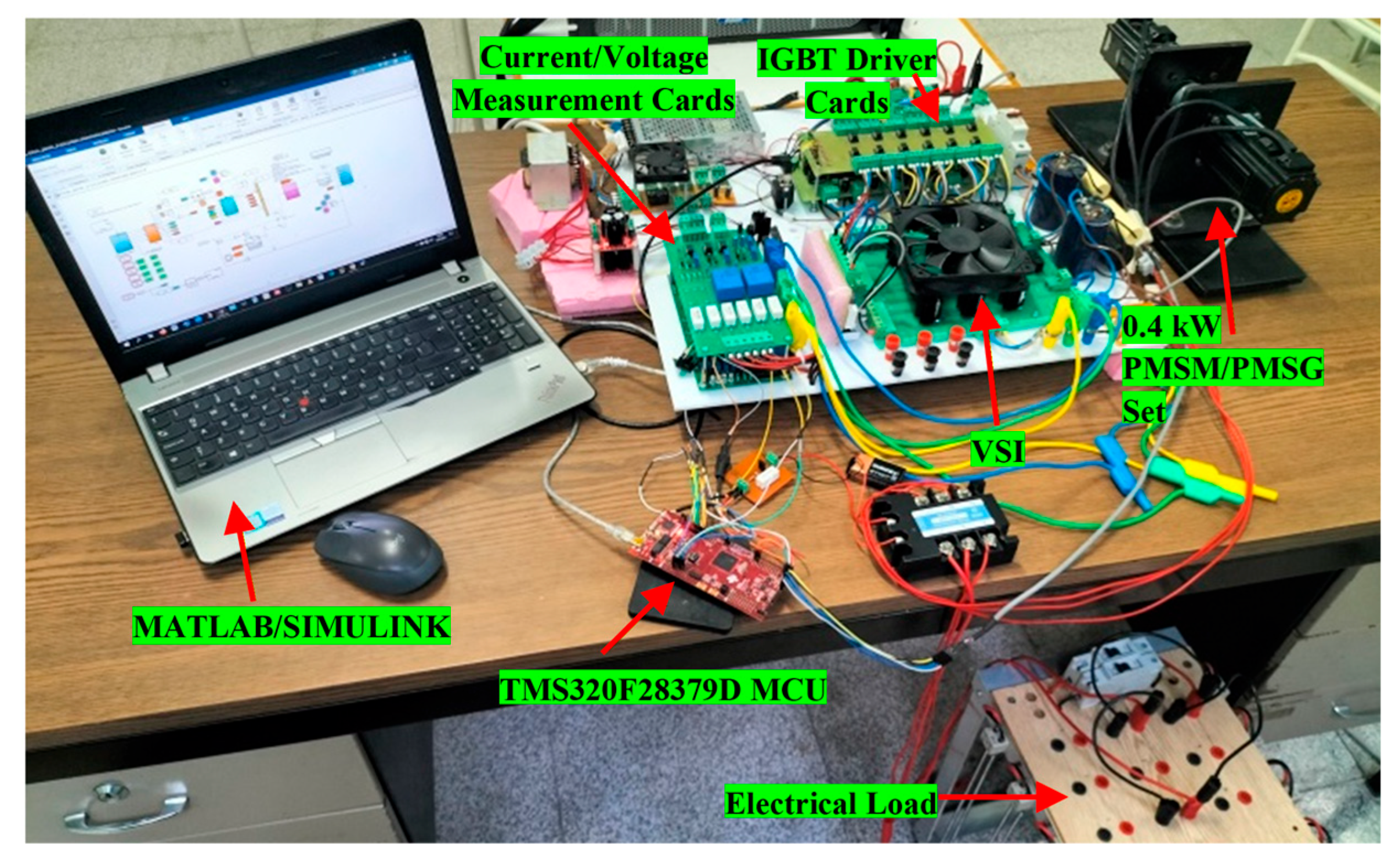
Figure 7 represents the experimental setup tested in the present investigation. The Texas Intrument-Dallas, TX, USA TI TMS320F28379D MCU is employed to execute control algorithms and generate PWM signals. The switching signals are optically isolated utilizing Broadcom Inc.-San Josa, CA, USA HCPL-3120 optocoupler integrated circuits. The LEM International SA-Meyrin, Switzerland LEM LV25-P and LEM LA25-P Hall effect sensors are used to measure voltages and currents, respectively. The system provides protection against abnormal voltages and currents using op-amp-based comparator circuits [45].

Table 3. PMSM parameters.

Parameters	Definition	Value
$P_n$	Nominal power	400 W
$V_n$	Nominal voltage	200 V
$I_n$	Nominal current	2.7 A
${\omega }_n$	Nominal speed	3000 rpm
$p_n$	Pole pair	4
$R_s$	Phase resistance	2.35 Ω
$L_{dq}$	dq axis inductance	6.5 × 10−3
$J$	Inertia	0.31 × 10−4 kgm2

presents the parameters of the two PMSMs with the same specifications used in the experiment. A motor generator set was created by coupling it to another motor with the same parameters.

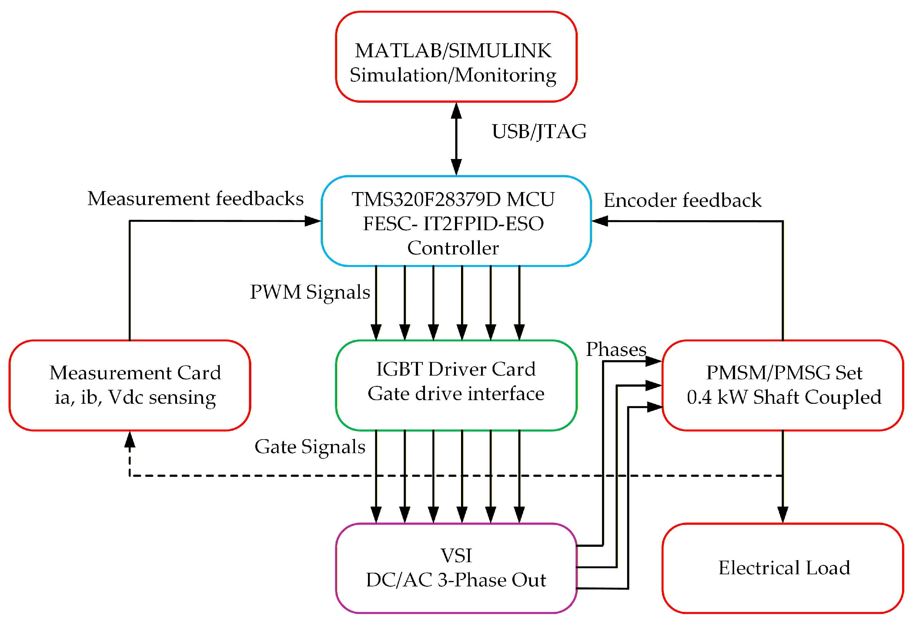
The principle connection diagram of the experimental setup shown in Figure 7 is provided in Figure 8. The laboratory setup constitutes a closed-loop motor drive system in which a digital signal processor (DSP)-based controller executes an advanced control algorithm—specifically a FESC-IT2FPID-ESO controller—to regulate the PMSM. The architecture is structured across four hierarchical functional layers: monitoring and simulation, control and processing, power conversion, and load/machine hardware. The host computer runs. Communication with the embedded controller is established via a USB/JTAG interface, enabling code deployment and live signal observation. The Texas Instruments dual-core C2000 Delfino DSP serves as the central embedded controller within the system. The FESC-IT2FPID-ESO control law, operating in real time, produces six-channel PWM signals that are then directed to the inverter. Simultaneously, it processes encoder feedback from the machine shaft to determine both rotor position and speed. Dedicated signal conditioning hardware is employed to determine the phase currents (i_a, i_b). These analog measurements are then converted and returned to the MCU as measurement feedback signals, thereby closing the inner current control loop. The gate driver board receives low-voltage PWM logic signals from the MCU and subsequently translates them into high-power gate drive signals appropriate for switching the IGBT devices in the inverter, thereby ensuring essential electrical isolation and level shifting. Finally, a three-phase, two-level voltage source inverter transforms the DC bus voltage into a variable-frequency, variable-amplitude three-phase AC output. A 0.4 kW PMSM and a PMSG are mechanically coupled via a common shaft. The PMSM operates in motoring mode, while the PMSG acts as a controllable mechanical load. An incremental encoder mounted on the shaft supplies rotor position feedback directly to the MCU.

4.1. Results of Simulations

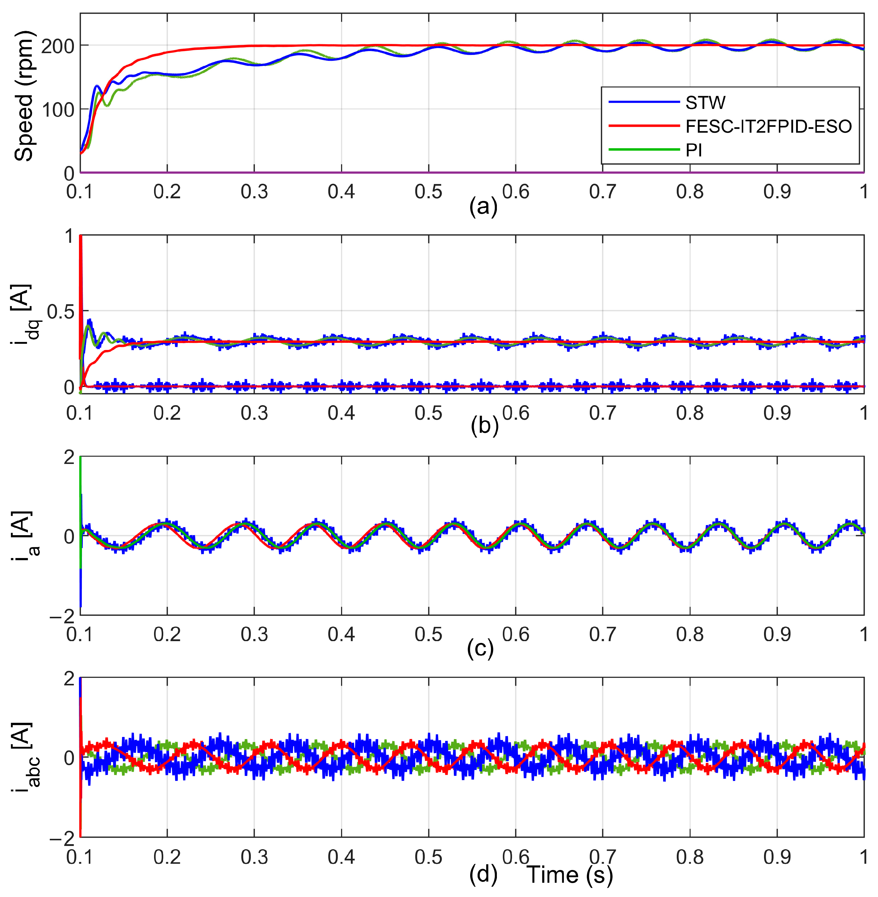
A simulation of the control system was conducted to provide insights for experimental investigations and provide an initial comparison with the experimental outcomes of the suggested controller structure in this article. In simulation investigations, the influence of cogging torque ripple and flux harmonics requires modeling via electromagnetic finite element analysis; therefore, these effects are disregarded, and an approximate model is employed. Current measurement inaccuracies, amplitude fluctuations, and offset errors are closely simulated to reflect the test system. Under these assumptions, the simulated responses of the PI, STW-SMC, and the proposed controller configuration are illustrated in the same graph for comparative analysis, as demonstrated in experimental tests.

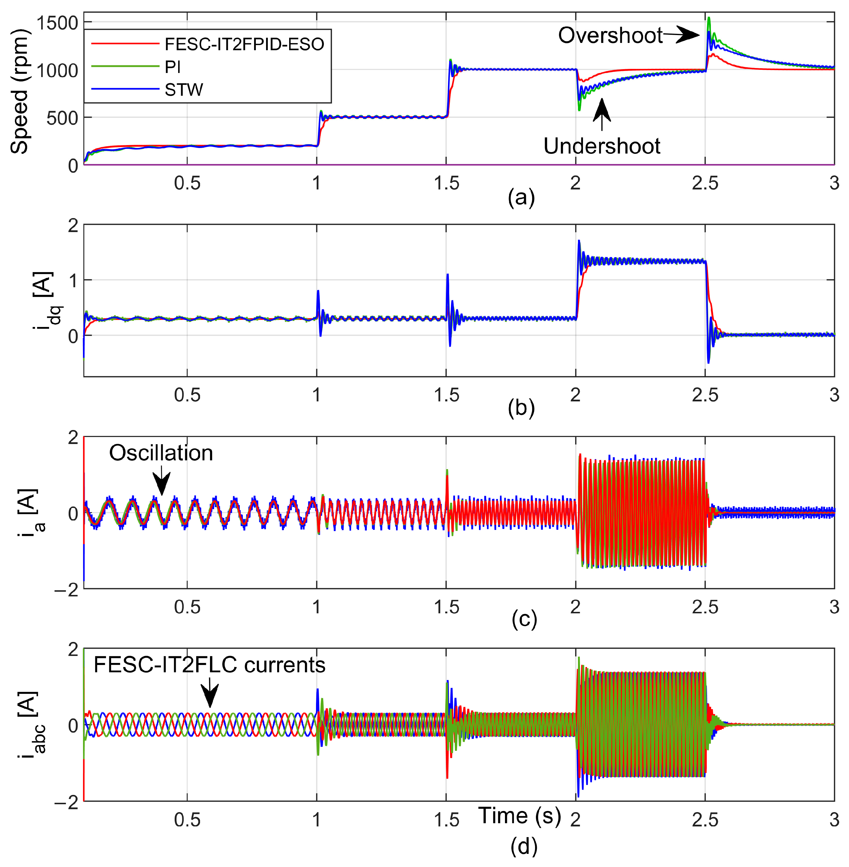
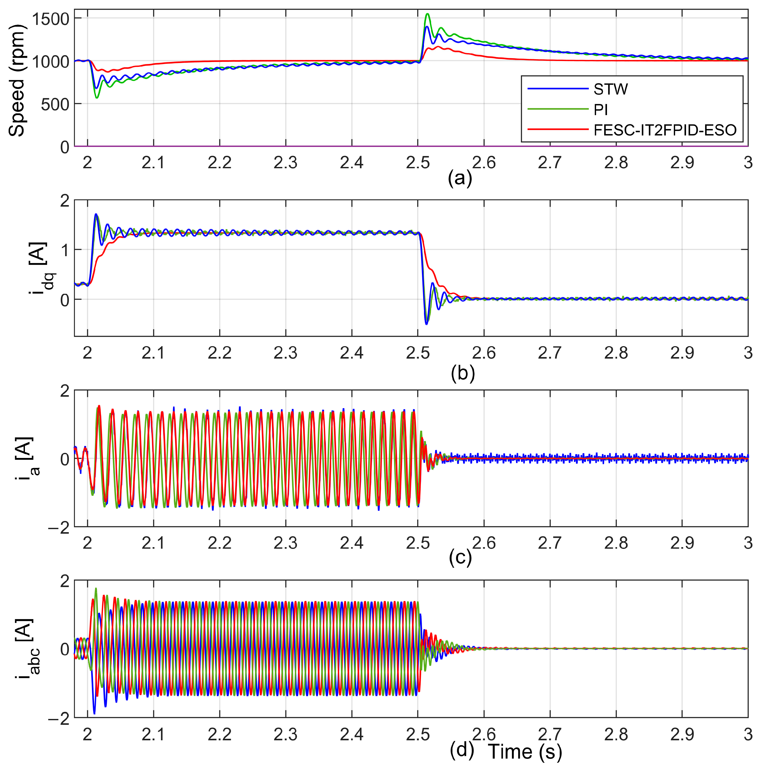
Figure 9 shows a comparative presentation of the simulation results for the controllers at low and medium set speeds, with one-second intervals, consistent with the experimental study conditions. The graphs show the currents on the speed, d and q axes, the a phase current, and the abc phase currents. As can be seen in the speed graphs, the proposed FESC-IT2FLC-ESO controller reaches the reference speed without overshoot in the low- and medium-speed regions. While the PI and STW controllers have better rise times than the approximate simulation model, they exhibit greater overshoot and oscillations in the speed and current graphs. In addition, more oscillation and ripple are noticeable in the STW controller responses due to chattering.

Figure 10 shows the zoomed-in dynamic responses of the three controllers between 0 and 1 s. At a reference speed of 200 rpm, the FESC-IT2FLC-ESO controller exhibits both the convergence of the reference value and an output response with minimal speed oscillation. The proposed controller produces a smoother current output than the PI and STW controllers, as it generates the q-axis reference current. The STW-SMC demonstrates a slower transient response during the initial acceleration phase and, once in the steady state, displays the highest speed ripple of all three controllers—an observation that is fully consistent with the settling time and disturbance amplitude figures reported in

Table 4. A performance comparison of the controllers.

Control Method	Low-Speed and No-Load Operation			Medium-Speed and Load Torque Operation
	Rise Time (s)	Settling Time (s)	Ripple Amplitude (rpm)-%	Rise Time (s)	Settling Time (s)	Overshoot (rpm)-%	Undershoot (rpm)-%	Ripple Amplitude (rpm)-%
PI	0.11	0.52	45–21.5%	0.090	0.71	73	260–26%	13–1.3%
STW-SMC	0.075	0.26	52–26%	0.054	0.19	51	190–19%	18–1.8%
FESC-TI2FPID-ESO	0.075	0.29	6–3%	0.076	0.25	0	26–2.6%	8.5–0.8%
FESC-TI2FPID-ESO ΔJ	0.076	0.30	13–6.5%	0.077	0.26	0	35–3.5%	12–1.2%

.

In Figure 11, when the speed and current graphs are examined at a reference speed of 1000 rpm under load torque, the proposed controllers yield much better output in terms of overshoot, undershoot, and oscillation. Numerical comparison values are provided in experimental studies.

4.2. Experimental Results

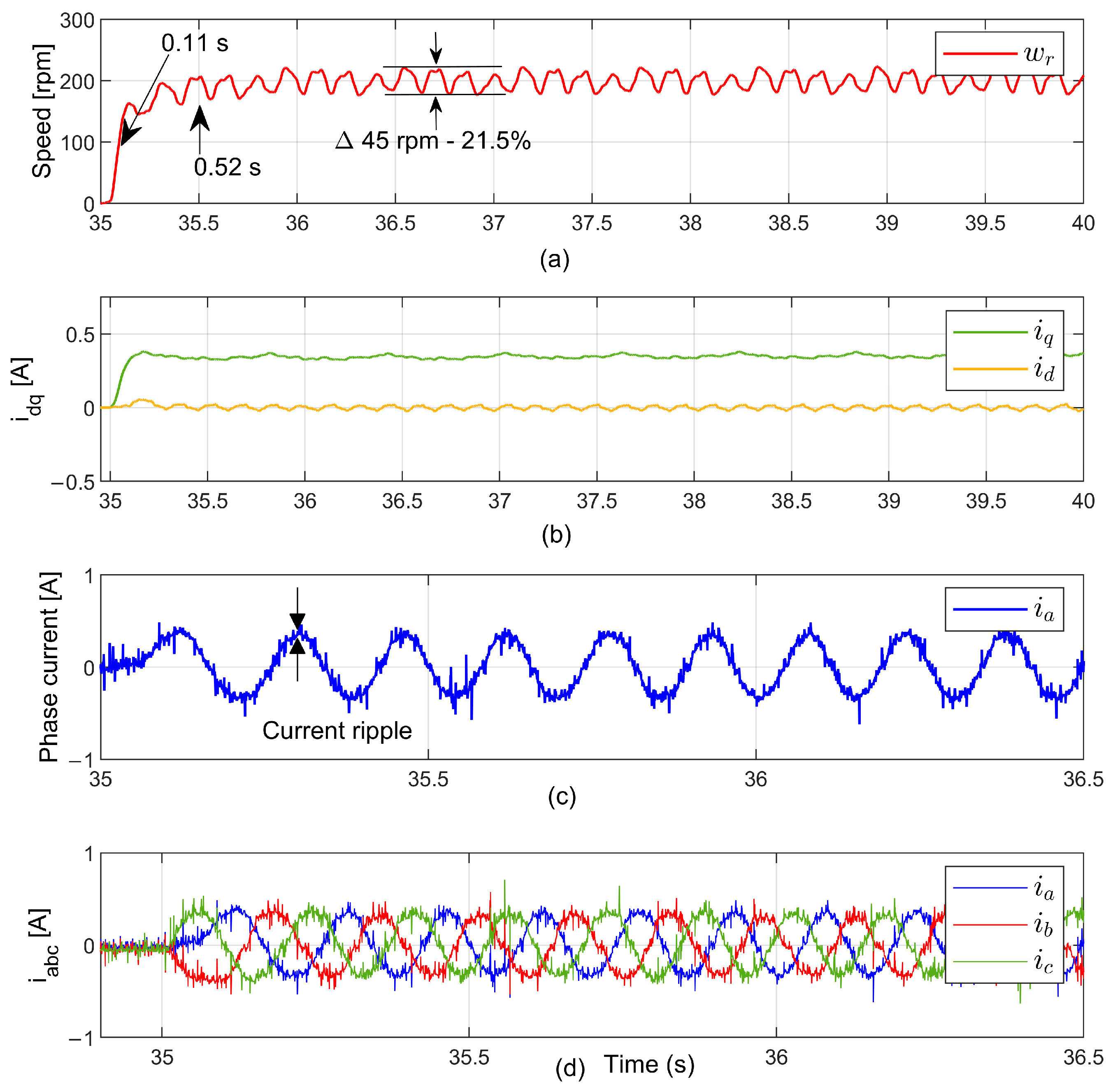
The experimental graphs of the PI and STW sliding mode controller performance are shown in Figure 12 and Figure 13, both for no-load operation and at 200 rpm low-speed operation. The speed oscillation of the PI controller shown in Figure 12 is about 45 rpm, 21.5%, given the performance indicated in Table 4.

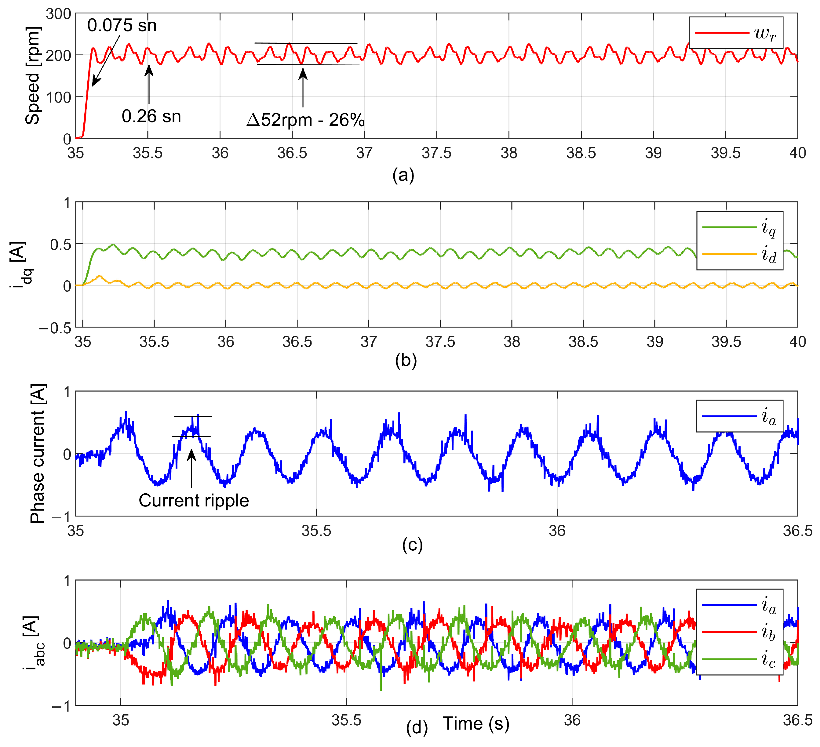
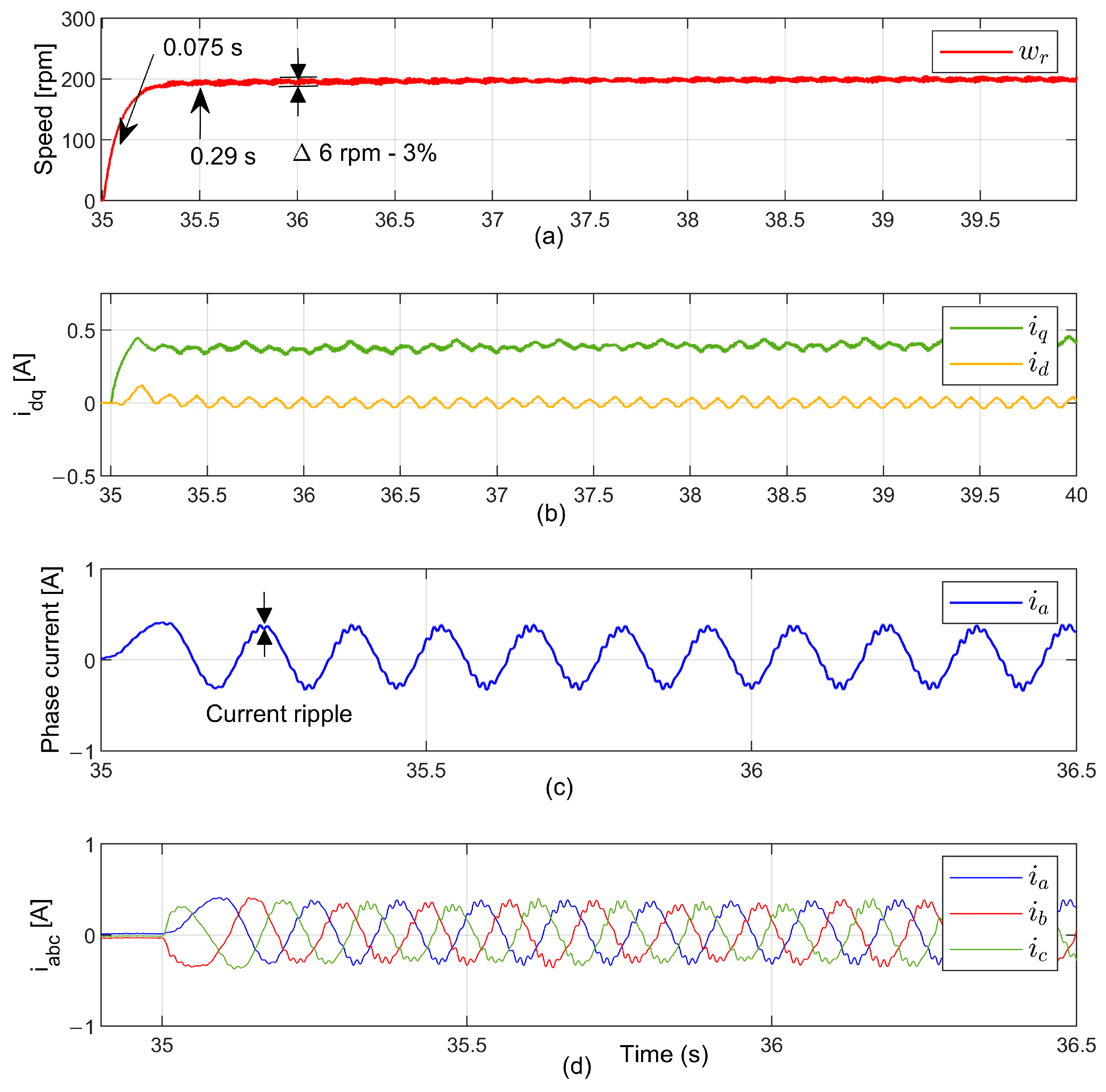
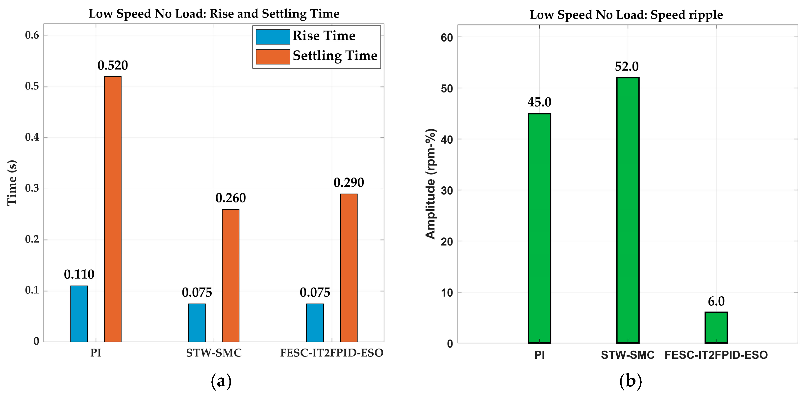
The STW sliding mode controller’s speed response, as shown in Figure 13, exhibits a fluctuation of about 52 rpm (26%). Since the speed controller’s output sets the q-axis current reference, the ripple in the phase currents is notable due to the high-speed fluctuations. This situation is similar for both the PI and STW sliding mode. Performance indicators such as rising time and settling time are also provided in Table 4. The STW sliding mode and FESC-IT2FPID-ESO controllers were found to have a similar rise time of 0.075 s under no-load operation, while the PI controller exhibited lower performance with a rise time of 0.11 s. None of the controllers exhibited overshoot at 200 rpm, a low operating speed. The FESC-IT2FPID-ESO controller’s speed and current responses at low-speed reference are presented in Figure 14.

Speed fluctuations in the graph are significantly mitigated by the combined effects of the IT2FPID controller’s dynamic response, the ESO’s effect, and the fast response ESC. In Figure 14, the fluctuation is shown to be only about 6 rpm (3%). The enhancement in the current response and the reduction in current ripple are also readily apparent, as the speed controller’s output is used as the current controller’s input reference value.

The significant improvement in speed fluctuations is compared in Figure 13 and Figure 14. The behavior of the ESO-based FESC-IT2FPID, PI, and STW controllers under load torque at a medium speed reference is depicted in Figure 15, Figure 16 and Figure 17.

The speed fluctuation was reduced from approximately 26% to 3% via the presented controller compared to other controllers. At low speed, when considering other performance indicators, the STW sliding mode controller yields similar results while demonstrating superior performance compared to the PI controller.

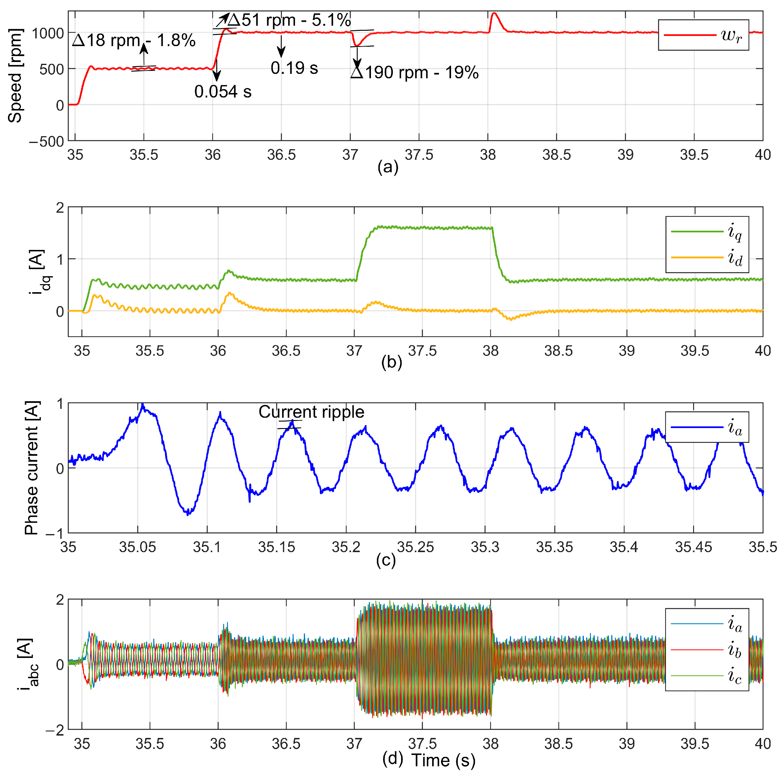
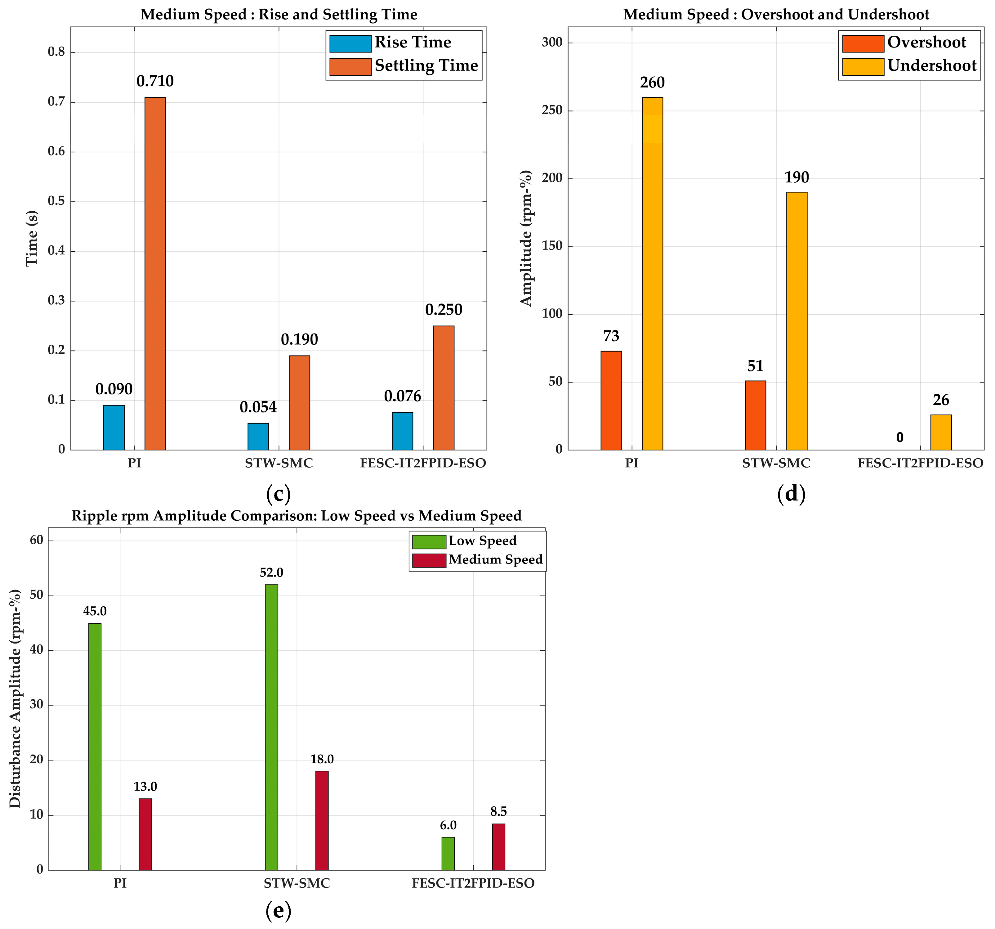
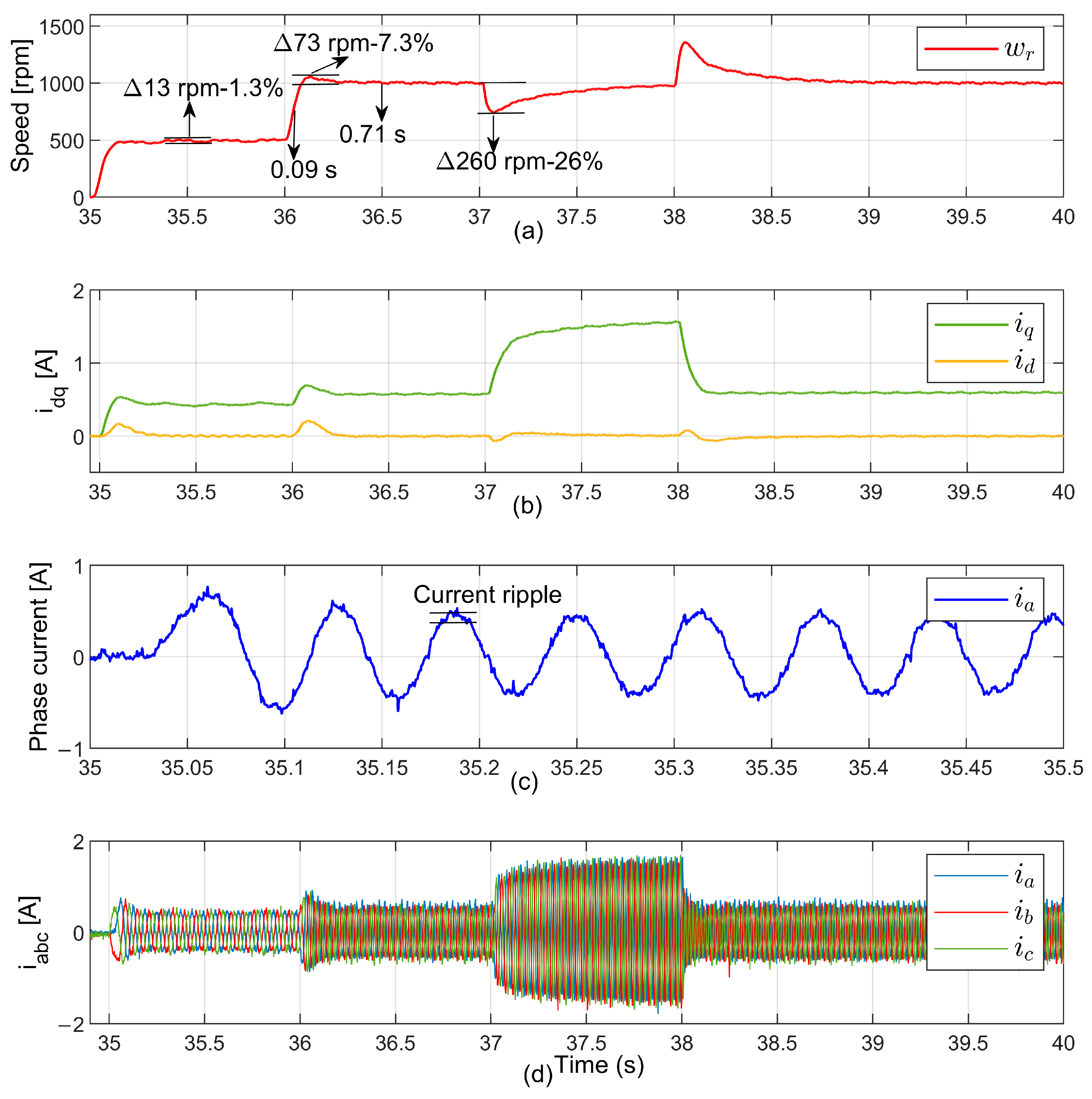
Cogging torque is particularly pronounced at low speeds, as mentioned in the Introduction and Modeling sections. Figure 15, Figure 16 and Figure 17 present the controller performance and speed ripple comparisons for all three controllers respectively. As the speed increases, the speed and current harmonics due to cogging torque and flux harmonics decrease. The fastest controller in terms of rise time and settling time was the STW controller, while the controller with the slowest speed response was the PI controller.

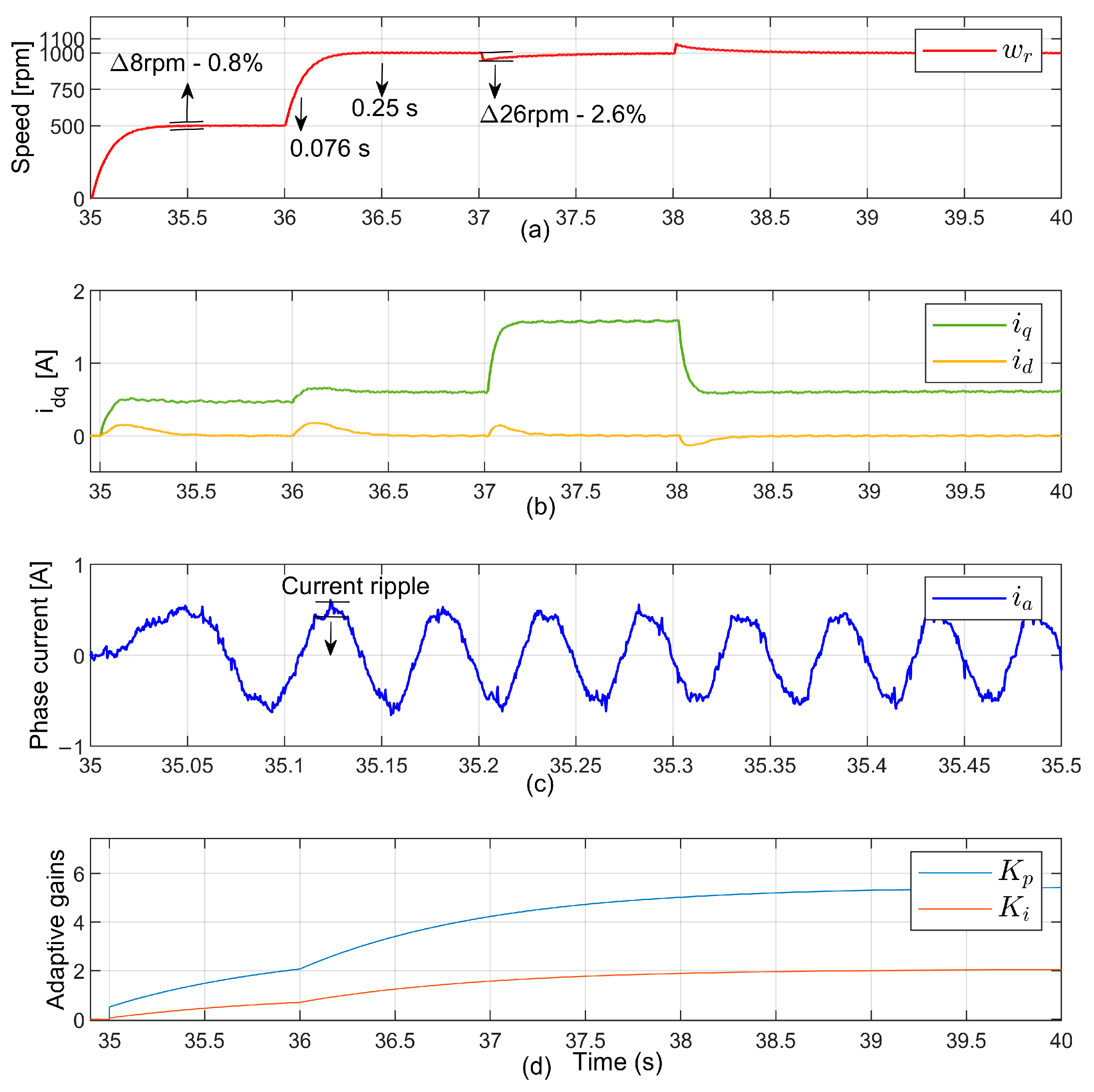
However, as shown in Table 4, while the PI and STW controllers exhibit high overshoots of 71% and 53%, respectively, the FESC-IT2FPID-ESO controller shows zero overshoot. In addition, during the operating period when the load moment is active, the PI and STW sliding mode controllers show speed responses that decrease by 26% and 19%, respectively. The proposed controller, on the other hand, has only a 2.6% undershoot effect in the speed response. Controllers exhibit different responses compared to each other in the medium-speed operating regions.

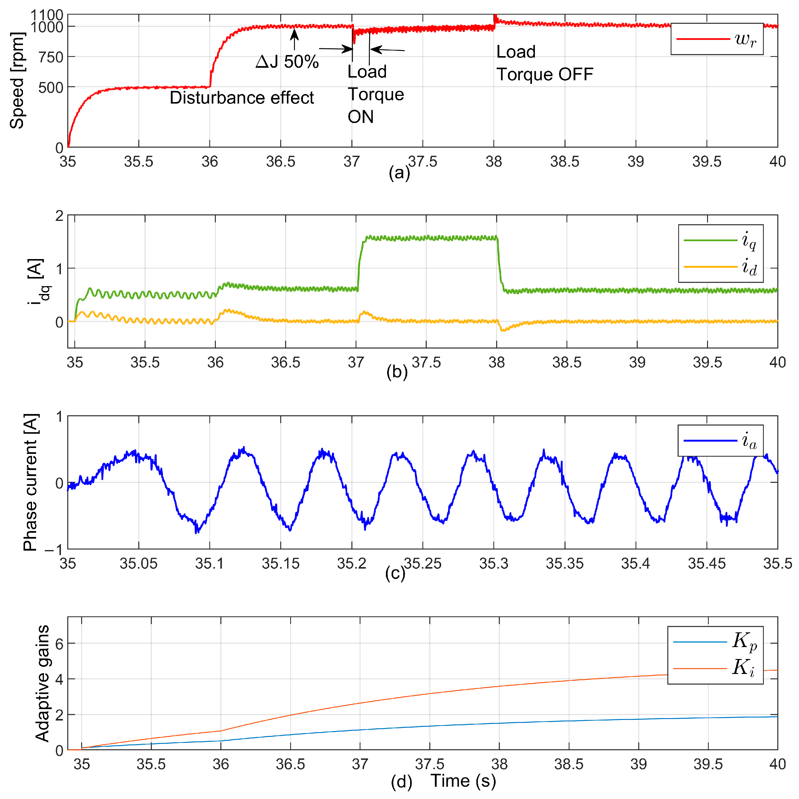
The experimental results of the 50% ΔJ inertia disturbance test presented in Figure 18 demonstrate that the proposed FESC-TI2FPID-ESO controller exhibits strong robustness against mechanical parameter uncertainties. In this case, a 50% increase in inertia under operational conditions results in no notable difference in the motor’s performance. The proposed controller also gives better results compared to the other two controllers in this case.

In Figure 17d and Figure 18d, the change in optimal gains adjusted online by the extremum-seeking search method varies with changes in load torque, speed, and ΔJ inertia. Thus, the optimal speed response is obtained without overshoot, regardless of whether it operates in the low- or medium-speed region. The ESC optimal gain controller is adjusted online to the ideal gain value in all situations with step references, load torque, and other internal and external disturbance effects to minimize speed errors. On the other hand, the ESO similarly generates an additional compensation response against all disturbance effects based on the speed error. During the moments when the load torque is applied and removed, the rapid recovery of the speed signal confirms that the ESO effectively predicted and suppressed the collective disruptive effects. When examining the d–q axis current responses, it is observed that during load transitions, the iq current increases as expected to meet the load moment, while the id current remains close to zero; this indicates that the integrity of the field-oriented control is maintained.

The proposed FESC-TI2FPID-ESO controller derives its performance from how three distinct methodological components work together. Each component has its own advantages. The interval type-2 fuzzy PID structure, with its secondary membership functions, offers more flexibility than type-1 fuzzy systems. This makes it better at handling system uncertainties and nonlinearities, such as cogging torque and friction at low speeds. The FESC mechanism addresses tuning burden by enabling the real-time, model-free online optimization of the IT2FPID parameters, thereby eliminating the need for precise system identification and allowing the controller to adapt dynamically to operating point changes—as evidenced by the near-zero overshoot and low settling times observed experimentally. Nevertheless, the convergence speed and stability of the extremum-seeking loop are sensitive to the perturbation signal amplitude and frequency, and the improper selection of these parameters may introduce oscillatory transients or slow adaptation, particularly under rapidly varying load conditions. The ESO complements both components by actively estimating and compensating for lumped disturbances—including unmodeled dynamics, parameter perturbations, and external load torques—in real time, which accounts for the dramatic reduction in disturbance amplitude (6–3% at low speed; 8.5–0.8% at medium speed) observed with the proposed method relative to PI and STW-SMC. Collectively, these three components form a complementary architecture in which the IT2FPID provides structural robustness, the FESC ensures autonomous parameter optimization, and the ESO delivers active disturbance rejection—yielding a controller that outperforms both conventional PI and sliding mode approaches across all evaluated metrics. The identified limitations point toward future research directions involving adaptive observer bandwidth tuning and computationally efficient fuzzy inference implementations.

In Table 4, the performance evaluation values of three different controllers used in this experimental study are presented. These controllers are the classical PI controller, the STW sliding mode controller, and the proposed parameter adaptive controller. The experiments focused on the low-speed region and the no-load condition to compare the controllers’ performance. The other operating field is the region where the load torque is applied at medium speeds.

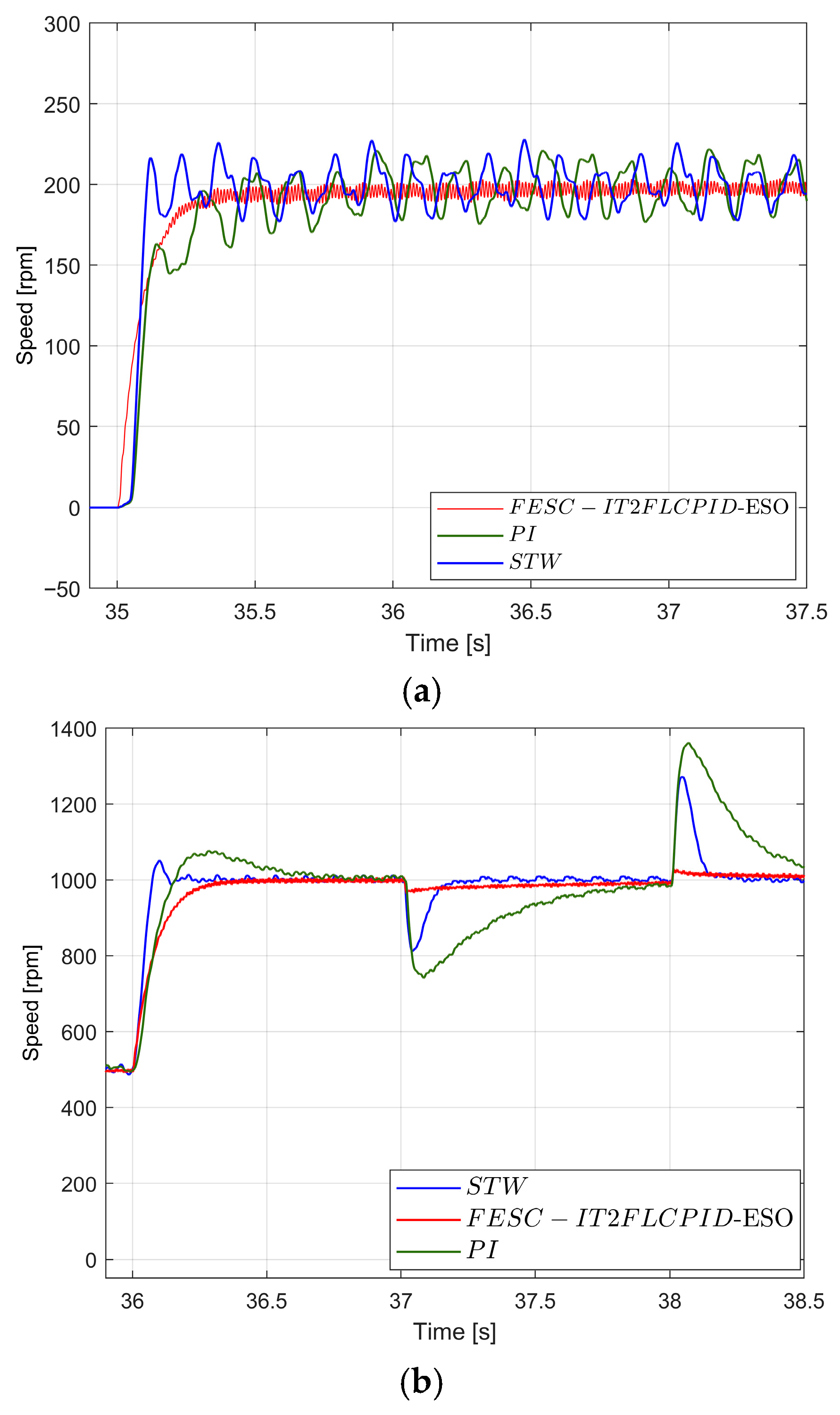
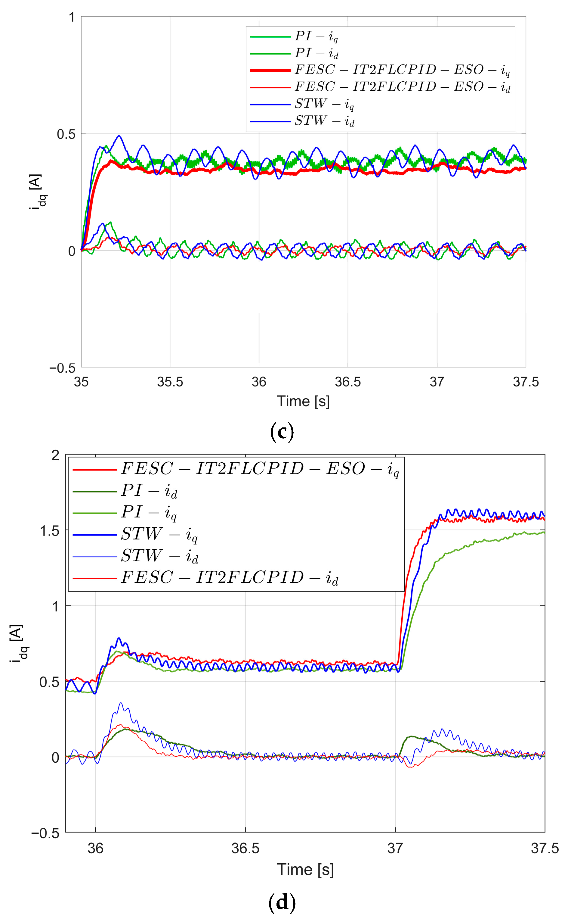
All comparisons are made in the previous graphs, with numerical values indicated in Table 2. These numerical values reveal many control criterion values. Figure 19a–d illustrate the low- and medium-speed operating regions, as well as the operating regions where instant load torque is applied, zoomed in for comparison purposes. It can be easily seen that the proposed online gain adaptive ESO-FESC-IT2FPID controller significantly suppresses oscillations and ripple in the speed response compared to the PI and STW controllers for speed and currents. Table 2 presents the performance values for comparison purposes. Figure 20a–d show the bar graphs of these performance values. Across all graphs, the proposed controller shows clear superiority in both performance and the reduction in speed fluctuations.

5. Conclusions

This study presents an approach using an extended state observer-based, fast response, extremum-seeking control interval type-2 fuzzy PID controller to reduce speed fluctuations at low speeds of the PMSM and improve dynamic response in the presence of other disturbances. This approach ensures the real-time adaptation of controller gains to mitigate the decline in control performance caused by the PMSM’s nonlinear characteristics and parameter fluctuations while also optimizing speed response fluctuations and instantaneous speed variations.

The results of this experiment show that the FESC-TI2FPID-ESO controller is much better at rejecting disturbances than other methods. The disturbance amplitude was reduced to only 6–3% under low-speed, no-load conditions. This was an improvement of about 87% over the PI controller (45–21.5%) and 88% over the STW-SMC (52–26%). This result is especially important because low-speed ripple suppression remains one of the hardest parts of PMSM control due to the strong effects of nonlinear friction and cogging torque. The proposed controller completely eliminated overshoot (0 rpm-%), whereas the PI and STW-SMC had overshoots of 73% and 51%, respectively. The undershoot response was also reduced significantly, from 260 to 26% for PI and 190 to 19% for STW-SMC to 26 to 2.6%. FESC-TI2FPID-ESO has a settling time of 0.25 s, which is competitive with STW-SMC’s settling time of 0.19 s. The strength of the suggested method against uncertainties in mechanical parameters was further tested using the FESC-TI2FPID-ESO ΔJ variant, which includes compensation for changes in inertia while the system is running. The ΔJ variant featured a small increase in disturbance amplitude (13–6.5% at low speed; 12–1.2% at medium speed) compared to the nominal FESC-TI2FPID-ESO. In summary, the FESC-TI2FPID-ESO controller provides a fast dynamic response, no overshoot, and improved disturbance rejection across many operating modes. The extended state observer’s integration enables the active compensation of lumped disturbances, and the fast extremum-seeking algorithm enables the real-time self-tuning of the IT2FPID parameters without requiring accurate system modeling.

Because of these features, the proposed scheme is well suited to real-world PMSM drive applications that require very precise speed control, such as robotics, electric vehicle traction, and industrial servo systems. The proposed solution has some limitations. The IT2FPID inference mechanism incurs substantial computational burden, a consequence of the type reduction process fundamental to interval type-2 fuzzy logic. The FESC loop’s ability to converge depends on the disturbance signal’s size and frequency. This is especially important when dealing with rapidly changing load profiles or a wide range of speed commands. To overcome these limitations, several improvements are suggested for future research. The IT2FPID structure will be refined by using computationally efficient type reduction algorithms, such as the Nie–Tan method. The ESO exhibits proficient disturbance compensation; however, the estimation bandwidth requires careful calibration to mitigate sensitivity to measurement noise, given that overly increased observer gains could induce closed-loop instability. Future research will explore adaptive observer gain scheduling methodologies to determine ESO bandwidth.

References

1. Chen, J.; Zhu, H.; Shu, T.; Cao, C.; Deng, Y. Improved Grey Wolf Optimizer and Backpropagation Neural Network for Fractional-Order Control of PMSM. Appl. Sci. 2026, 16, 1516. [Google Scholar] [CrossRef]
2. Xu, Y.; Huang, Z.; Liu, D. Research on Position Tracking Performance Optimization of Permanent Magnet Synchronous Motors Based on Improved Active Disturbance Rejection Control. Appl. Sci. 2025, 15, 10467. [Google Scholar] [CrossRef]
3. Bai, W.; Kuang, Y.; Xu, Z.; Wang, Y.; Hua, X. Research on Vibration Characteristics of Electric Drive Systems Based on Open-Phase Self-Fault-Tolerant Control. Appl. Sci. 2025, 15, 8707. [Google Scholar] [CrossRef]
4. Nakao, N.; Akatsu, K. Suppressing Pulsating Torques. IEEE Ind. Appl. Mag. 2014, 20, 33–44. [Google Scholar] [CrossRef]
5. Betin, F.; Capolino, G.; Casadei, D.; Kawkabani, B. Trends in Electrical Machines Control. IEEE Ind. Electron. Mag. 2014, 8, 43–55. [Google Scholar] [CrossRef]
6. Flieller, D.; Nguyen, N.; Wira, P.; Sturtzer, G.; Abdeslam, D.; Mercklé, J. A Self-Learning Solution for Torque Ripple Reduction for Nonsinusoidal Permanent-Magnet Motor Drives Based on Artificial Neural Networks. IEEE Trans. Ind. Electron. 2014, 61, 655–666. [Google Scholar] [CrossRef]
7. Park, D.; Kim, K. Parameter-Independent Online Compensation Scheme for Dead Time and Inverter Nonlinearity in IPMSM Drive Through Waveform Analysis. IEEE Trans. Ind. Electron. 2014, 61, 701–707. [Google Scholar] [CrossRef]
8. Lam, B.H.; Xu, J.X.; Panda, S.K. Reduction of Periodic Speed Ripples in PM Synchronous Motors Using Iterative Learning Control. In Proceeding IEEE IECON; IEEE: Piscataway, NJ, USA, 2000; pp. 1406–1411. [Google Scholar] [CrossRef]
9. Islam, R.; Husain, I.; Fardoun, A.; Laughlin, K.M. Permanent Magnet Synchronous Motor Magnet Designs with Skewing for Torque Ripple and Cogging Torque Reduction. IEEE Trans. Ind. Appl. 2009, 45, 152–160. [Google Scholar] [CrossRef]
10. Houari, A.; Bouabdallah, A.; Djerioui, A.; Machmoum, M. An Effective Compensation Technique for Speed Smoothness at Low-Speed Operation of PMSM Drives. IEEE Trans. Ind. Appl. 2018, 54, 647–655. [Google Scholar] [CrossRef]
11. Feng, G.; Lai, C.; Kar, N.C. A Closed-Loop Fuzzy-Logic-Based Current Controller for PMSM Torque Ripple Minimization Using the Magnitude of Speed Harmonic as the Feedback Signal. IEEE Trans. Ind. Electron. 2017, 64, 2642–2653. [Google Scholar] [CrossRef]
12. Wang, Y.; Li, P.; Shen, J.; Jiang, C. Adaptive Periodic Disturbance Observer Based on Fuzzy Logic Compensation for Speed Fluctuation Suppression of PMSM Under Periodic Loads. IEEE Trans. Ind. Appl. 2024, 60, 5751–5762. [Google Scholar] [CrossRef]
13. Kim, K.H.; Youn, M.J. A Nonlinear Speed Control for a PM Synchronous Motor Using a Simple Disturbance Estimation Technique. IEEE Trans. Ind. Electron. 2002, 49, 524–535. [Google Scholar] [CrossRef]
14. Grčar, B.; Cafuta, P.; Žnidarič, M.; Gausch, F. Nonlinear Control of Synchronous Servo Drive. IEEE Trans. Control Syst. Technol. 1996, 4, 177–184. [Google Scholar] [CrossRef]
15. Li, S.; Zhou, M.; Yu, X. Design and Implementation of Terminal Sliding Mode Control Method for PMSM Speed Regulation System. IEEE Trans. Ind. Inform. 2013, 9, 1879–1891. [Google Scholar] [CrossRef]
16. Zhang, X.; Sun, L.; Sun, L.; Zhao, K. Nonlinear Speed Control for PMSM System Using Sliding-Mode Control and Disturbance Compensation Techniques. IEEE Trans. Power Electron. 2013, 28, 1358–1365. [Google Scholar] [CrossRef]
17. Sun, Z.; Deng, Y.; Wang, J.; Li, H.; Cao, H. Improved Cascaded Model-Free Predictive Speed Control for PMSM Speed Ripple Minimization Based on Ultra-Local Model. ISA Trans. 2023, 143, 666–677. [Google Scholar] [CrossRef]
18. Mora, A.; Orellana, A.; Juliet, J.; Cardenas, R. Model Predictive Torque Control for Torque Ripple Compensation in Variable-Speed PMSMs. IEEE Trans. Ind. Electron. 2016, 63, 4584–4592. [Google Scholar] [CrossRef]
19. Liu, X.; Zhang, C.; Li, K.; Zhang, Q. Robust Current Control-Based Generalized Predictive Control with Sliding Mode Disturbance Compensation for PMSM Drives. ISA Trans. 2017, 71, 542–552. [Google Scholar] [CrossRef] [PubMed]
20. Errouissi, R.; Al-Durra, A.; Muyeen, S.M.; Leng, S. Continuous-Time Model Predictive Control of a Permanent Magnet Synchronous Motor Drive with Disturbance Decoupling. IET Electr. Power Appl. 2017, 11, 697–706. [Google Scholar] [CrossRef]
21. Wang, S.; Xia, C.; Gu, X.; Chen, W. A Novel FCS-Model Predictive Control Algorithm with Duty Cycle Optimization for Surface-Mounted PMSM. In Proceeding IET PEMD; IEEE: Piscataway, NJ, USA, 2014; pp. 1–6. [Google Scholar]
22. Zhang, Y.; Gao, S. Simultaneous Optimization of Voltage Vector and Duty Cycle in Model Predictive Torque Control of PMSM Drives. In Proceeding ICEMS; IEEE: Piscataway, NJ, USA, 2014; pp. 3338–3344. [Google Scholar] [CrossRef]
23. Zhou, J.; Wang, Y. Adaptive Backstepping Speed Controller Design for a Permanent Magnet Synchronous Motor. IET Electr. Power Appl. 2002, 149, 165–172. [Google Scholar] [CrossRef]
24. Jan, R.M.; Tseng, C.S.; Liu, R.J. Robust PID Control Design for Permanent Magnet Synchronous Motor: A Genetic Approach. Electr. Power Syst. Res. 2008, 78, 1161–1168. [Google Scholar] [CrossRef]
25. Wang, G.J.; Fong, C.T.; Chang, K.J. Neural-Network-Based Self-Tuning PI Controller for Precise Motion Control of PMAC Motors. IEEE Trans. Ind. Electron. 2001, 48, 408–415. [Google Scholar] [CrossRef]
26. Chaoui, H.; Sicard, P.; Gueaieb, W. ANN-Based Adaptive Control of Robotic Manipulators with Friction and Joint Elasticity. IEEE Trans. Ind. Electron. 2009, 56, 3174–3187. [Google Scholar] [CrossRef]
27. Chaoui, H.; Gueaieb, W. Type-2 Fuzzy Logic Control of a Flexible-Joint Manipulator. J. Intell. Robot. Syst. 2008, 51, 159–186. [Google Scholar] [CrossRef]
28. Liang, Q.; Mendel, J.M. Introduction to Type-2 TSK Fuzzy Logic Systems. In Proceeding IEEE FUZZ-IEEE; IEEE: Piscataway, NJ, USA, 1999; pp. 1534–1539. [Google Scholar]
29. Liang, Q.; Mendel, J.M. Interval Type-2 Fuzzy Logic Systems: Theory and Design. IEEE Trans. Fuzzy Syst. 2000, 8, 535–550. [Google Scholar] [CrossRef] [PubMed]
30. Song, Z.; Zhang, Z.; Komurcugil, H.; Lee, C.H.T. Controller-Based Periodic Disturbance Mitigation Techniques for Three-Phase Two-Level Voltage-Source Converters. IEEE Trans. Ind. Inform. 2021, 17, 6553–6568. [Google Scholar] [CrossRef]
31. Xia, C.; Ji, B.; Yan, Y. Smooth Speed Control for Low-Speed High-Torque Permanent-Magnet Synchronous Motor Using Proportional-Integral-Resonant Controller. IEEE Trans. Ind. Electron. 2015, 62, 2123–2134. [Google Scholar] [CrossRef]
32. Pan, Z.; Dong, F.; Zhao, J.; Wang, L.; Wang, H.; Feng, Y. Combined Resonant Controller and Two-Degree-of-Freedom PID Controller for PMSLM Current Harmonics Suppression. IEEE Trans. Ind. Electron. 2018, 65, 7558–7568. [Google Scholar] [CrossRef]
33. Wang, X.; Jiang, C.; Zhuang, F.; Lee, C.H.T.; Chan, C.C. A Harmonic Injection Method Equivalent to the Resonant Controller for Speed Ripple Reduction of PMSM. IEEE Trans. Ind. Electron. 2022, 69, 9793–9803. [Google Scholar] [CrossRef]
34. Li, J.; Zhang, L.; Luo, L.; Li, S. Extended State Observer Based Current-Constrained Controller for a PMSM System in Presence of Disturbances: Design, Analysis and Experiments. Control Eng. Pract. 2023, 132, 105412. [Google Scholar] [CrossRef]
35. Taleshian, T.; Noei, A.R.; Sadati, J. Perturbation Observer Design Based on Extremum Seeking Control: An Analytical Insight. Trans. Inst. Meas. Control 2024, 46, 886–898. [Google Scholar] [CrossRef]
36. Liu, J.; Li, H.; Deng, Y. Torque Ripple Minimization of PMSM Based on Robust ILC via Adaptive Sliding Mode Control. IEEE Trans. Power Electron. 2018, 33, 3655–3671. [Google Scholar] [CrossRef]
37. Tian, M.; Wang, B.; Yu, Y.; Dong, Q.; Xu, D. Robust Adaptive Resonant Controller for PMSM Speed Regulation Considering Uncertain Periodic and Aperiodic Disturbances. IEEE Trans. Ind. Electron. 2023, 70, 3362–3372. [Google Scholar] [CrossRef]
38. Tong, W.; Zhao, T.; Duan, Q.; Zhang, H.; Mao, Y. Non-Singleton Interval Type-2 Fuzzy PID Control for High Precision Electro-Optical Tracking System. ISA Trans. 2022, 120, 258–270. [Google Scholar] [CrossRef]
39. Praharaj, M.; Sain, D.; Mohan, B.M. Development, Experimental Validation, and Comparison of Interval Type-2 Mamdani Fuzzy PID Controllers with Different Footprints of Uncertainty. Inf. Sci. 2022, 601, 374–402. [Google Scholar] [CrossRef]
40. Qiao, W.Z.; Mizumoto, M. PID-Type Fuzzy Controller and Parameters Adaptive Method. Fuzzy Sets Syst. 1996, 78, 23–35. [Google Scholar] [CrossRef]
41. Killingsworth, N.; Krstić, M. Auto-Tuning of PID Controllers via Extremum Seeking. In Proceeding American Control Conference; IEEE: Piscataway, NJ, USA, 2005; pp. 2251–2256. [Google Scholar] [CrossRef]
42. Guay, V.A.M. Robust Adaptive MPC for Systems with Exogenous Disturbances. IFAC Proc. Vol. 2009, 42, 00038. [Google Scholar]
43. Guay, M.; Dochain, D. A Proportional-Integral Extremum-Seeking Controller. Automatica 2017, 77, 61–67. [Google Scholar] [CrossRef]
44. Bajracharya, C.; Marta, M.; Are, S.; Undeland, T. Understanding of Tuning Techniques of Converter Controllers for VSC-HVDC. In Proceedings of the Nordic Workshop on Power and Industrial Electronics, Helsinki, Finland, 9–11 June 2008; pp. 1–8. [Google Scholar]
45. Sezen, S.; Kılıç, F. Visual Re-Initialization Model Development Methodology for Solving Problems Regarding Metaheuristic Algorithm-Based MPPT Applications. Electr. Power Compon. Syst. 2024, 52, 1597–1615. [Google Scholar] [CrossRef]
Figure 1. A diagram of the PMSM speed control block.
Applsci 16 03093 g001
Figure 2. A schematic of the interval type-1 and -2 fuzzy PID controller.
Applsci 16 03093 g002
Figure 3. Interval type-1 and -2 fuzzy PID controller schematics.
Applsci 16 03093 g003
Figure 4. T1FLC and IT2FLC membership functions and controller surface. (a) T1FLC membership functions. (b) T1FLC surface. (c) IT2FLC surface. (d) IT2FLC surface.
Applsci 16 03093 g004
Figure 5. Gain adaptive fast extremum-seeking IT2FPID controller schematic.
Applsci 16 03093 g005
Figure 6. Extended state observer schematic.
Applsci 16 03093 g006
Figure 7. The experimental setup.
Applsci 16 03093 g007
Figure 8. A diagram of the experimental setup block.
Applsci 16 03093 g008
Figure 9. PI, STW, and FESC-IT2FPID-ESO controllers’ dynamic responses: (a) speeds and (b) dq axis currents, (c) a phase current, and (d) abc phase currents.
Applsci 16 03093 g009
Figure 10. The PI, STW, and FESC-IT2FPID-ESO controllers’ dynamic responses for the low-speed region: (a) speeds, (b) dq axis currents, (c) a phase current, and (d) abc phase currents.
Applsci 16 03093 g010
Figure 11. PI, STW, and FESC-IT2FPID-ESO controllers’ dynamic responses for medium-speed region: (a) speeds, (b) dq axis currents, (c) a phase current, and (d) abc phase current.
Applsci 16 03093 g011
Figure 12. PI control of PMSM for low-speed region experimental graphs: (a) speed, (b) dq axis currents, (c) a phase current, and (d) abc phase currents.
Applsci 16 03093 g012
Figure 13. STW control of PMSM for low-speed region experimental graphs: (a) speed, (b) dq axis currents, (c) a phase current, and (d) abc phase currents.
Applsci 16 03093 g013
Figure 14. FESC-IT2FPID ESO control of PMSM for low-speed region experimental graphs: (a) speed, (b) dq axis currents, (c) a phase current, and (d) abc phase currents.
Applsci 16 03093 g014
Figure 15. PI control of PMSM under load torque for medium-speed region; (a) speed, (b) dq axis currents, (c) a phase current, and (d) abc phase currents.
Applsci 16 03093 g015
Figure 16. STW sliding mode control of PMSM under load torque for medium-speed region: (a) speed, (b) dq axis currents, (c) a phase current, and (d) abc phase currents.
Applsci 16 03093 g016
Figure 17. FESC-IT2FPID-ESO control of PMSM under load torque for medium-speed region: (a) speed, (b) dq axis currents, (c) a phase current, and (d) abc phase currents.
Applsci 16 03093 g017
Figure 18. FESC-IT2FPID-ESO control of PMSM under load torque and inertia variation for medium-speed region: (a) speed, (b) dq axis currents, (c) a phase current, and (d) abc phase currents.
Applsci 16 03093 g018
Figure 19. A speed comparison of the PI, STW sliding mode, and ESO-FESC-IT2FPID controllers: (a) low speed, (b) medium speed, (c) low-speed currents, and (d) medium-speed currents.
Applsci 16 03093 g019aApplsci 16 03093 g019b
Figure 20. PI, STW sliding mode, and ESO-FESC-IT2FPID controller performance comparison bar graphs: (a) low-speed rise and settling time; (b) low-speed oscillation, (c) low-speed rise and settling time, (d) medium overshoot and undershoot, and (e) medium-speed oscillation.
Applsci 16 03093 g020aApplsci 16 03093 g020b