Structure-Aware Feature Descriptor with Multi-Scale Side Window Filtering for Multi-Modal Image Matching

Abstract

Traditional image feature matching methods often fail to achieve satisfactory performance on multimodal remote sensing images (MRSIs), mainly due to significant nonlinear radiometric distortion (NRD) and complex geometric deformation caused by different imaging mechanisms. The key to successful MRSI matching lies in preserving high-frequency edge structures that are robust to geometric deformation, while overcoming nonlinear intensity mappings induced by NRD. To address these challenges, this paper proposes a novel high-precision matching framework, termed structure-aware feature descriptor with multi-scale side window filtering (SA-SWF). The proposed framework consists of three stages: (1) an anisotropic morphological scale space is constructed based on multi-scale side window filtering to strictly preserve geometric edges, and feature points are extracted using a multi-scale adaptive structure tensor with sub-pixel refinement to ensure high localization precision; (2) a structure-aware feature descriptor is constructed by integrating gradient reversal invariance and entropy-weighted attention mechanisms, rendering the multi-modal description highly robust against contrast inversion and noise; and (3) a coarse-to-fine robust matching strategy is established to progressively refine correspondences from descriptor-space matching to strict sub-pixel geometric verification, thereby minimizing alignment errors. Experiments on 60 multimodal image pairs from six categories, including infrared-infrared, optical–optical, infrared–optical, depth–optical, map–optical, and SAR–optical datasets, demonstrate that SA-SWF consistently outperforms seven state-of-the-art competitors. Across all six dataset categories, SA-SWF achieves a 100% success rate, the highest average number of correct matches (356.8), and the lowest average root mean square error (1.57 pixels). These results confirm the superior robustness, stability, and geometric accuracy of SA-SWF under severe radiometric and geometric distortions.

1. Introduction

Multimodal image matching aims to identify accurate corresponding points between images acquired from different sensors, spectral bands, viewpoints, or acquisition times. It is a fundamental step in the automated generation of photogrammetric and remote sensing products and directly affects a wide range of downstream applications, including change detection, image mosaicking, aerial triangulation, visual localization, image fusion, and three-dimensional reconstruction [1,2]. However, multimodal remote sensing image (MRSI) matching remains highly challenging because images captured by heterogeneous imaging mechanisms usually exhibit severe nonlinear radiometric distortion (NRD), local texture inconsistency, speckle contamination, and complicated geometric deformation [3]. These factors often cause conventional matching methods to produce only a limited number of reliable correspondences or even fail completely.

In recent years, substantial efforts have been devoted to multimodal image matching. Existing methods have improved robustness from different perspectives, such as similarity measurement, invariant feature extraction, phase-based representation, and deep neural network learning. Nevertheless, two key difficulties remain unresolved. First, under strong cross-modal radiometric inconsistency, many descriptors cannot maintain stable structural representation, especially in the presence of contrast inversion or weak texture regions. Second, conventional isotropic scale-space construction tends to blur corners and edges, which degrades the repeatability and localization accuracy of keypoints under multimodal conditions. Therefore, developing a matching framework that can simultaneously preserve structural edges, suppress modality-specific noise, and construct radiometrically robust descriptors is still an important research problem.

For MRSI, structural information is generally more stable than raw intensity information across modalities and therefore provides an effective basis for robust correspondence establishment [4]. In addition, anisotropic filtering strategies have shown strong potential for preserving meaningful geometric structures during multi-scale analysis, while entropy-based weighting provides a feasible way to highlight informative regions and suppress unreliable background responses. Motivated by these observations, we propose a novel high-precision multimodal image matching framework entitled structure-aware feature descriptor with multi-scale side window filtering (SA-SWF).

The working principle of SA-SWF is summarized as follows. First, a multi-scale side-window-filtering-based anisotropic morphological scale space is constructed to preserve structural edges while suppressing radiometric noise, and repeatable keypoints are extracted by a multi-scale adaptive structure tensor detector with sub-pixel refinement. Second, a structure-aware feature descriptor is built by combining gradient reversal invariance and entropy-weighted attention, so that stable structural cues can be retained under severe cross-modal intensity variations. Finally, initial correspondences are obtained in descriptor space and then refined in geometric space through robust homography estimation, leading to accurate multimodal registration.

The main contributions of this article are summarized as follows:

(1)

An anisotropic morphological scale space is constructed based on multi-scale side window filtering to strictly preserve geometric edges while suppressing noise. Within this framework, a multi-scale adaptive structure tensor detector with sub-pixel refinement is employed to extract a greater number of repeatable corner and edge points, ensuring high localization precision.

(2)

A structure-aware feature descriptor is proposed by integrating gradient reversal invariance and entropy-weighted attention mechanisms. This design enables the descriptor to adaptively emphasize informative structural edges while suppressing textureless background noise, thereby achieving strong robustness against contrast inversion and radiometric inconsistency.

(3)

A coarse-to-fine robust matching strategy is established to realize the transition from descriptor-space screening to strict sub-pixel geometric refinement. Comprehensive evaluations on six multimodal datasets, including infrared–infrared, optical–optical, infrared–optical, depth–optical, map–optical, and SAR–optical image pairs, demonstrate that the proposed method achieves superior accuracy and robustness compared with existing state-of-the-art approaches.

2. Related Work

Existing multimodal image matching methods can generally be divided into three categories: area-based methods, feature-based methods, and deep learning-based methods.

2.1. Area-Based Methods

Area-based methods establish correspondences by directly measuring the similarity between local image patches. Representative similarity measures include normalized cross-correlation (NCC) [5], mutual information (MI) [6,7,8], and histogram of oriented phase congruency (HOPC) [9]. These methods are attractive because they avoid explicit feature detection and can work well when the geometric discrepancy between image pairs is small. However, most area-based approaches are highly sensitive to large rotations, scale variation, and local nonrigid deformation. In addition, exhaustive similarity search over dense local windows often leads to high computational cost, which limits their applicability in large-scale remote sensing scenarios.

2.2. Feature-Based Methods

Feature-based methods perform matching by detecting salient keypoints and constructing local descriptors. Classical methods such as the scale-invariant feature transform (SIFT) [10], PSO-SIFT [11], and affine-SIFT (ASIFT) [12] mainly address geometric variations through scale or affine invariance. Although effective for same-modality or weakly heterogeneous images, these methods generally suffer from poor robustness under strong NRD because they rely heavily on local gradient magnitude and orientation distributions.

To alleviate radiometric inconsistency, many researchers have explored frequency–domain or phase-based descriptors. Typical examples include the radiation-variation-insensitive feature transform (RIFT) [13], the log-Gabor histogram descriptor (LGHD) [14], the histogram of weighted phase (HOWP) [15], the histogram of spectral consistency (HOSC) [16], and HAPCG [17]. These methods improve robustness to modality-dependent intensity variation by exploiting phase congruency, log-Gabor responses, or phase-based structural information. However, they may still be limited in scenarios involving large geometric transformation, weak texture, severe speckle noise, or insufficient structural distinctiveness.

2.3. Deep Learning-Based Methods

Deep learning has substantially enriched the methodological framework of multimodal image matching. Early methods based on convolutional neural networks (CNNs) [18,19] learned modality-invariant feature embeddings from paired samples. Subsequent studies introduced more sophisticated architectures, such as multi-relation attention networks [20], CM-Net [21], MatchFormer [22], and SemLA [23], to improve contextual modeling and feature correspondence under large appearance gaps. Although these methods achieve promising performance on specific benchmarks, they usually depend on large-scale labeled training data and may suffer from limited generalization when applied to unseen modalities, acquisition conditions, or scene types [24,25].

2.4. Structural Representation for Multimodal Matching

For multimodal remote sensing images, structural features are often more stable than raw intensity values and therefore provide an effective basis for robust matching [4]. Previous studies have shown that anisotropic diffusion mechanisms can generate different responses at corners, edges, and flat regions, which is beneficial for structural feature extraction [26]. However, conventional isotropic Gaussian smoothing and many standard diffusion strategies tend to blur edges and corners in deeper scale-space layers, reducing keypoint repeatability and localization precision. Side window filtering (SWF) [27] offers an attractive alternative because it preserves edge and corner structures more effectively during smoothing. On the descriptor side, traditional structural representations, such as histogram of oriented gradients (HOG) [28] and gradient location and orientation histogram (GLOH) [29], are not sufficiently robust to severe cross-modal radiometric inconsistency, especially under contrast inversion [30]. Meanwhile, self-similarity and entropy-based weighting have shown potential for enhancing descriptor distinctiveness by emphasizing informative local structures and suppressing low-confidence regions [31,32,33].

In summary, existing methods still face a trade-off between structural preservation, radiometric robustness, and geometric accuracy. This motivates us to develop a unified multimodal matching framework that combines edge-preserving anisotropic scale-space construction, structure-aware descriptor design, and robust geometric refinement.

3. Materials and Methods

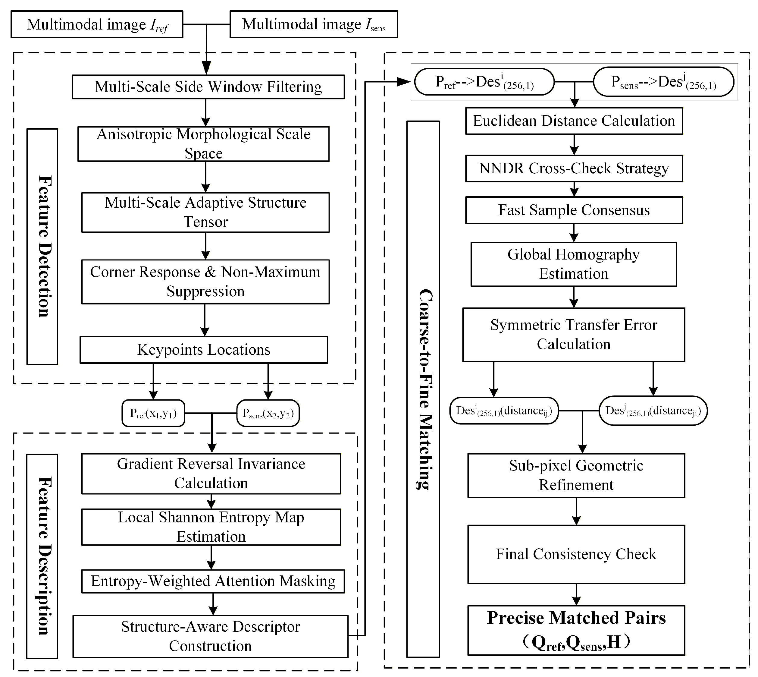
In this study, we propose a novel framework entitled structure-aware feature descriptor with multi-scale side window filtering (SA-SWF) to effectively address the challenges of NRD and geometric deformation in multimodal image matching. As shown in Figure 1, the proposed method integrates three core components to achieve high-precision registration. First, a detection framework based on multi-scale side window filtering (MS-SWF) is designed to construct an anisotropic scale space that strictly preserves edge structures and enables repeatable keypoint extraction. Second, a structure-aware feature descriptor (SE-GLOH) is developed by incorporating gradient reversal invariance and entropy-weighted attention to capture robust structural details against intensity variations. Finally, a coarse-to-fine matching strategy is employed to minimize alignment errors through descriptor screening, geometric verification, and sub-pixel refinement. For clarity, the three modules in Figure 1 correspond to feature detection, feature description, and coarse-to-fine matching, respectively.

3.1. Multi-Scale Side Window Filtering and Sub-Pixel Detection

To extract repeatable keypoints under complex radiometric conditions, we abandon traditional isotropic Gaussian smoothing. Instead, we introduce a detection module centered on multi-scale side window filtering (MS-SWF) and multi-scale adaptive structure tensor (MS-AST). As illustrated in the feature-detection branch of Figure 1, this module consists of multi-scale side window filtering, anisotropic morphological scale-space construction, multi-scale structure tensor analysis, corner response evaluation, non-maximum suppression, and sub-pixel keypoint localization.

3.1.1. Construction of Multi-Scale Side Window Filtering

The core of our scale space generation is the side window filtering technique, which suppresses noise while strictly preserving geometric edges. For a pixel $\mathbf{p}=(x,y)$, we define a set of eight oriented local side windows $\mathrm{\Omega }={\left\{W_k\right\}}_{k=1}^8$. The anisotropic response $L(\mathbf{p},s)$ at scale s is modeled as a local optimization problem:

$$L(\mathbf{p},s)={\mu }_{k^{\ast }}\left(\mathbf{p}\right),\mathrm{s}.\mathrm{t}.k^{\ast }=arg\underset{k\in \{1,\dots ,8\}}{min}{\parallel L(\mathbf{p},s-1)-{\mu }_k\left(\mathbf{p}\right)\parallel }_2^2$$

(1)

where $L(\mathbf{p},s)$ denotes the filtered intensity at pixel $\mathbf{p}$ and scale level s, $L(\mathbf{p},s-1)$ is the response from the previous scale, ${\mu }_k\left(\mathbf{p}\right)$ denotes the average intensity within the k-th side window $W_k$, and $k^{\ast }$ is the index of the optimal side window that minimizes the local reconstruction error. This formulation is inspired by the original side window filtering strategy [27] and is extended here to multi-scale structural feature detection for multimodal matching.

In implementation, the filter is iteratively applied to grayscale images using a side-window radius parameter. The default number of scales is set to 3, and the base radius is initialized as 1. For each scale, the radius increases with scale level so that the resulting anisotropic morphological scale space progressively suppresses high-frequency noise while preserving stable geometric boundaries. 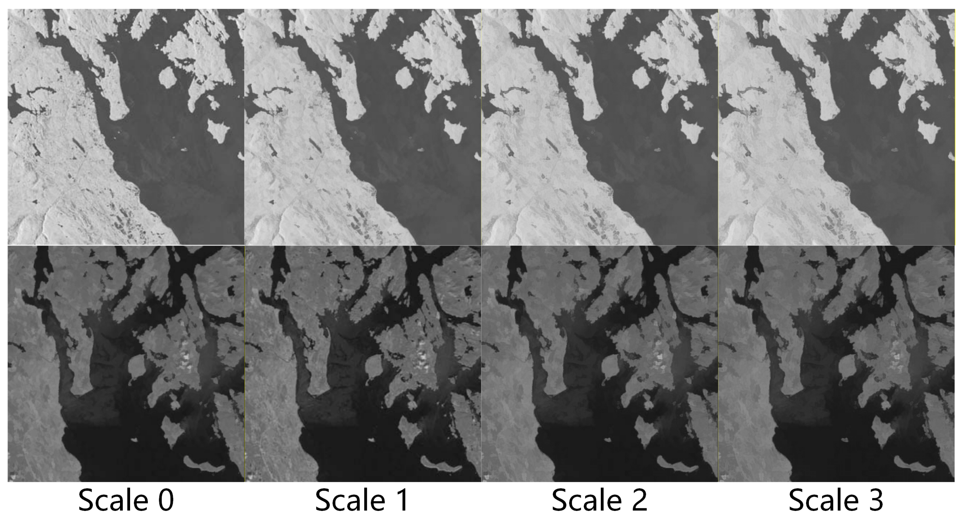Figure 2 shows that the proposed MS-SWF effectively suppresses speckle or thermal noise while retaining strong structures such as coastlines and river boundaries. This edge-preserving characteristic is pivotal for accurate feature localization in the subsequent detection stage.

3.1.2. Multi-Scale Adaptive Structure Tensor Detection with Sub-Pixel Refinement

Based on the MS-SWF manifold, we employ the structure tensor to quantify feature saliency. The moment matrix $\mathbf{M}\left(\mathbf{p}\right)$ is calculated as:

$$\mathbf{M}\left(\mathbf{p}\right)=G_{\sigma }\ast \left(\nabla L\left(\mathbf{p}\right)·\nabla L{\left(\mathbf{p}\right)}^{\top }\right)$$

(2)

where $\nabla L\left(\mathbf{p}\right)$ denotes the image gradient at pixel $\mathbf{p}$ in the MS-SWF scale space, $G_{\sigma }$ is a Gaussian kernel with standard deviation $\sigma$, and ∗ denotes convolution. Robust corners are identified using the Shi–Tomasi criterion [34], i.e., ${\lambda }_{min}\left(\mathbf{M}\right)>\tau$. The structure tensor formulation follows the classical second-moment matrix representation widely used in corner detection and local structure analysis [35].

In the actual implementation, keypoints are extracted on a grid-constrained basis to improve spatial coverage. Specifically, each image is divided into a $3\times 3$ grid, and a Shi–Tomasi detector is applied independently in each cell using qualityLevel$=0.01$ and minDistance$=5$. The maximum number of retained keypoints is set to 5000 over all scales. Corner responses are ranked scale by scale, and non-maximum suppression is performed implicitly through local peak selection in the detector output, thereby suppressing unstable and redundant responses.

To meet high-precision requirements, we further implement a sub-pixel refinement step. The precise coordinates $\mathbf{q}$ are derived by minimizing the orthogonal gradient error within a local neighborhood $\mathcal{N}$:

$$\mathbf{q}={\left(\sum _{{\mathbf{p}}_i\in \mathcal{N}}\nabla I\left({\mathbf{p}}_i\right)\nabla I{\left({\mathbf{p}}_i\right)}^{\top }\right)}^{-1}\left(\sum _{{\mathbf{p}}_i\in \mathcal{N}}(\nabla I{\left({\mathbf{p}}_i\right)}^{\top }{\mathbf{p}}_i)\nabla I\left({\mathbf{p}}_i\right)\right)$$

(3)

where $\mathcal{N}$ denotes the local neighborhood around the candidate keypoint, $\nabla I\left({\mathbf{p}}_i\right)$ is the image gradient at pixel ${\mathbf{p}}_i$, and $\mathbf{q}$ is the refined sub-pixel coordinate. This closed-form solution refines localization accuracy from pixel-level to sub-pixel level, significantly reducing the root mean square error (RMSE) of registration. This closed-form refinement is derived in this work based on local orthogonal gradient consistency.

3.2. Structure-Aware Feature Descriptor

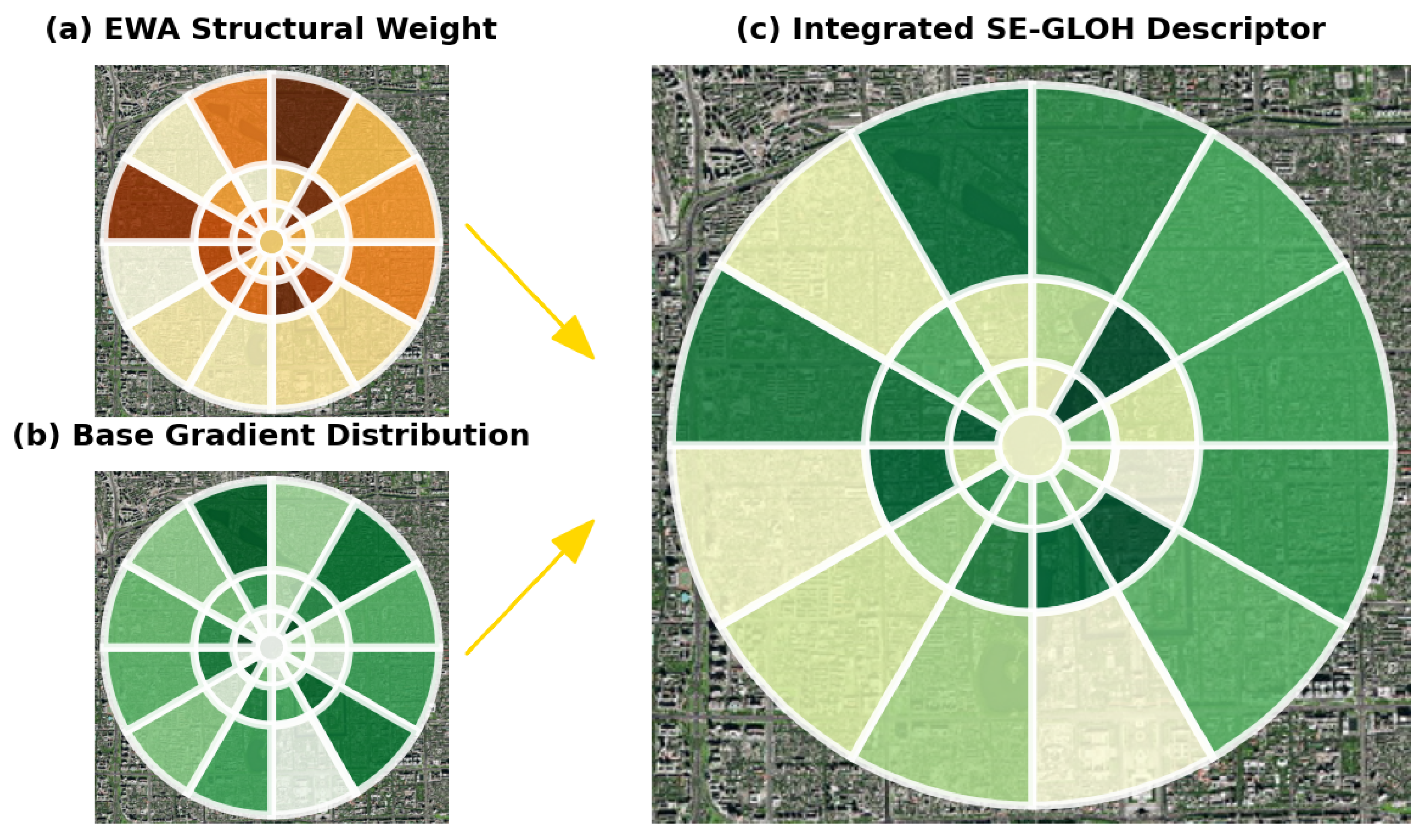
To robustly describe cross-modal features under complex radiometric distortions, we propose a structure-aware feature descriptor, termed SE-GLOH. Unlike traditional descriptors, SE-GLOH explicitly captures stable structural information by integrating gradient reversal invariance (GRI) and entropy-weighted attention (EWA). The descriptor construction process consists of four main steps: polarity-invariant gradient calculation, local Shannon entropy estimation, entropy-guided attention weighting, and final structure-aware descriptor encoding. A visual illustration of the descriptor construction process is provided in Figure 3.

First, to address intensity inversion, we define a unified gradient field ${\mathbf{g}}_{inv}$ that is invariant to polarity changes. We select the dominant structural edge direction as:

$${\mathbf{g}}_{inv}\left(\mathbf{p}\right)=\mathbb{I}(\parallel \nabla I^{+}\parallel >\parallel \nabla I^{-}\parallel )·\nabla I^{+}+\mathbb{I}(\parallel \nabla I^{+}\parallel \le \parallel \nabla I^{-}\parallel )·(-\nabla I^{-})$$

(4)

where $\nabla I^{+}$ and $\nabla I^{-}$ denote the gradient responses under the original and reversed intensity polarity, respectively, and $\mathbb{I}(·)$ is the indicator function. In implementation, the gradient field is computed using the Scharr operator in both intensity directions, and the larger-magnitude response is retained at each location. As shown in Figure 3b, this GRI operation enforces a consistent orientation energy distribution across the log-polar grid, ensuring that geometric structures remain stable despite contrast reversals.

However, raw gradients often contain background noise. To highlight informative structures, we introduce the local Shannon entropy $\mathcal{H}\left(\mathbf{x}\right)$ as a soft attention mask, as visualized in Figure 3a. The final descriptor bin value $h_b$ is calculated as:

$$h_b={\int }_{\mathbf{x}\in {\mathrm{bin}}_b}\parallel {\mathbf{g}}_{inv}{\left(\mathbf{x}\right)\parallel ·\mathcal{G}(\parallel \mathbf{x}-\mathbf{c}\parallel )·(1+\alpha \mathcal{H}\left(\mathbf{x}\right))}^{\beta }d\mathbf{x}$$

(5)

where $h_b$ denotes the value of the b-th descriptor bin, $\mathbf{x}$ is the pixel location within the support region, ${\mathbf{g}}_{inv}\left(\mathbf{x}\right)$ is the polarity-invariant gradient at $\mathbf{x}$, $\mathcal{G}(\parallel \mathbf{x}-\mathbf{c}\parallel )$ is the spatial weighting function centered at $\mathbf{c}$, $\mathcal{H}\left(\mathbf{x}\right)$ denotes the local Shannon entropy, and $\alpha$ and $\beta$ are hyperparameters controlling the strength of entropy-guided attention.

Specifically, the spatial layout of SE-GLOH follows a log-polar coordinate system consisting of $R=3$ radial rings and $S=12$ angular sectors, plus a central circular region, resulting in a total of $N=37$ spatial bins. To capture fine-grained directional information, the gradient orientations within each spatial bin are further quantized into $B=8$ histogram bins. Consequently, the raw SE-GLOH descriptor is represented as a $37\times 8=296$-dimensional feature vector. In the actual implementation, dominant orientations are estimated within a radius of 15 pixels using a 36-bin orientation histogram, and square-root normalization is applied to the histogram vector to improve robustness.

The visual impact of this weighting is demonstrated in Figure 3c. By modulating the base gradient with entropy, the descriptor effectively suppresses textureless regions (low entropy) while emphasizing high-contrast structural edges (high entropy). This attention mechanism ensures that the final feature representation is both discriminative and robust to multimodal distortions.

3.3. Coarse-to-Fine Robust Matching

To achieve robust registration, we adopt a hierarchical strategy transitioning from descriptor space to geometric space. The matching module includes descriptor projection, Euclidean distance calculation, nearest-neighbor screening, sample consensus, global homography estimation, symmetric transfer error evaluation, sub-pixel geometric refinement, and final consistency verification.

Coarse Matching (Feature Space): An initial set of putative matches ${\mathcal{S}}_{init}$ is established by minimizing the Euclidean distance in the structure-aware descriptor space:

$${\mathcal{S}}_{init}=\left\{(i,j)\mid \parallel {\mathbf{f}}_i^r-{\mathbf{f}}_j^s{\parallel }_2=\underset{k}{min}{\parallel {\mathbf{f}}_i^r-{\mathbf{f}}_k^s\parallel }_2\right\}$$

(6)

where ${\mathcal{S}}_{init}$ denotes the initial set of putative correspondences, and ${\mathbf{f}}_i^r$ and ${\mathbf{f}}_j^s$ denote the descriptors of the i-th keypoint in the reference image and the j-th keypoint in the sensed image, respectively. This coarse matching step follows the standard nearest-neighbor matching principle widely used in local feature correspondence [10]. In implementation, the 296-dimensional SE-GLOH descriptors are first projected to a lower-dimensional space using principal component analysis (PCA), with the retained dimensionality set to 256, and Euclidean nearest-neighbor search is then performed by a KD-tree. To further suppress many-to-one ambiguity, one-to-one uniqueness is enforced by retaining only the lowest-distance match for each candidate in the sensed image.

Fine Matching: Using the sub-pixel coordinates obtained in the multi-scale adaptive structure tensor detection stage, we refine the matches by estimating the optimal homography matrix $\widehat{\mathbf{H}}$ via RANSAC. We minimize the symmetric transfer error with a strict geometric threshold $T_{geo}$:

$$\widehat{\mathbf{H}}=arg\underset{\mathbf{H}}{min}\sum _{(i,j)\in {\mathcal{S}}_{init}}\rho \left(\parallel {\mathbf{q}}_j^s-\mathbf{H}{\tilde{\mathbf{q}}}_i^r{\parallel }_{\mathrm{\Sigma }}^2,T_{geo}\right)$$

(7)

where ${\tilde{\mathbf{q}}}_i^r$ denotes the homogeneous representation of the refined keypoint in the reference image, ${\mathbf{q}}_j^s$ is the corresponding sub-pixel coordinate in the sensed image, $\mathrm{\Sigma }$ denotes the geometric weighting term, and $\rho (·,T_{geo})$ is a robust loss function with geometric threshold $T_{geo}$. This formulation follows the standard robust homography estimation framework based on RANSAC [36] and projective geometric verification [37]. In implementation, the homography is estimated by RANSAC with a reprojection threshold of $3.0$ pixels. After homography estimation, all putative matches are re-evaluated by geometric consistency, and correspondences with reprojection error not larger than $3.0$ pixels are retained as geometrically consistent inliers. For quantitative evaluation, RMSE is also computed using correspondences with reprojection error not larger than $3.0$ pixels. This step enforces strict sub-pixel geometric alignment, ensuring the final registration accuracy.

3.4. Implementation Details

All experiments were implemented in Python 3.8. The number of MS-SWF scales was set to 3, and the base filter radius was initialized as 1 and increased with scale level. In feature detection, each image was divided into a $3\times 3$ grid, and the maximum number of retained keypoints was set to 5000. The Shi–Tomasi detector was applied with qualityLevel$=0.01$ and minDistance$=5$. In the descriptor construction stage, local entropy was computed with a window radius of 9 and 16 quantization bins. The descriptor was organized using a log-polar layout with $R=3$ radial rings, $S=12$ angular sectors, and $B=8$ orientation bins, resulting in a 296-dimensional raw feature vector. Dominant orientation estimation was performed with a radius of 15 pixels and 36 orientation bins. For efficient matching, PCA was used to reduce the descriptor dimension to 256. During geometric verification, the RANSAC threshold was set to $3.0$ pixels, and both homography-consistency checking and RMSE statistics were conducted using correspondences with reprojection error not larger than $3.0$ pixels.

3.5. Algorithmic Summary

Algorithm 1 summarizes the complete pipeline of the proposed SA-SWF method.

Algorithm 1: SA-SWF for multimodal image matching.

Input: Reference image $I_{ref}$ and sensed image $I_{sens}$ Output: Precise matched pairs $({\mathbf{Q}}_{ref},{\mathbf{Q}}_{sens},\mathbf{H})$ 1: Convert the input images to grayscale. 2: Construct multi-scale side-window-filtered images and generate the anisotropic morphological scale spaces. 3: Detect candidate keypoints using the multi-scale adaptive structure tensor in a grid-constrained manner. 4: Perform corner response selection and retain spatially distributed keypoints. 5: Refine retained keypoints to sub-pixel locations. 6: Compute polarity-invariant gradients using forward and reversed intensity responses. 7: Estimate local Shannon entropy maps and generate entropy-weighted attention masks. 8: Construct 296-dimensional SE-GLOH descriptors for all detected keypoints. 9: Project descriptors to 256 dimensions using PCA. 10: Perform KD-tree-based Euclidean nearest-neighbor matching with one-to-one uniqueness screening. 11: Estimate the global homography by RANSAC. 12: Re-evaluate correspondences using reprojection error and retain geometrically consistent matches. 13: Output the final precise matched pairs.

4. Results

To rigorously evaluate the performance of the proposed SA-SWF method, we conducted comprehensive qualitative and quantitative comparisons using sixty multimodal image pairs. We benchmarked our approach against seven representative baselines, spanning classical algorithms to state-of-the-art (SOTA) deep learning methods: SIFT, HOPC, HAPCG, RIFT, CMM-Net, MatchFormer [22], and SemLA [23]. For a fair comparison, all experiments were conducted using the official source codes, and the deep learning-based methods utilized the original pre-trained weights provided by their respective authors. Furthermore, for all compared methods, the Random Sample Consensus (RANSAC) algorithm with an inlier threshold of three pixels was applied to reject outliers.

To quantitatively assess registration performance, we employ three standard metrics widely used in multimodal image matching, namely root mean square error (RMSE), number of correct matches (NCM), and success rate (SR) [38]. A match is deemed correct if its reprojection error under the ground truth homography $\mathbf{H}$ is below three pixels ($ϵ=3$), and an image pair is classified as successfully registered if it retains at least 10 correct matches ($\tau =10$). The calculations for these metrics are formulated as follows:

$$\begin{array}{cc}\hfill & \mathrm{RMSE}=\sqrt{{\displaystyle \frac{1}{N_{in}}}\sum _{i=1}^{N_{in}}{\parallel {\mathbf{x}}_i-\mathbf{H}{\mathbf{y}}_i\parallel }_2^2}\hfill \end{array}$$

(8)

$$\begin{array}{cc}\hfill & \mathrm{NCM}=\sum _{j=1}^M\mathbb{I}\left(\parallel {\mathbf{x}}_j-\mathbf{H}{\mathbf{y}}_j{\parallel }_2<ϵ\right)\hfill \end{array}$$

(9)

$$\begin{array}{cc}\hfill & \mathrm{SR}={\displaystyle \frac{1}{K}}\sum _{k=1}^K\mathbb{I}\left({\mathrm{NCM}}_k\ge \tau \right)\times 100\%\hfill \end{array}$$

(10)

where $N_{in}$ denotes the number of correct matches (inliers); M is the total number of putative matches; K represents the total number of image pairs in the dataset category; and $\mathbb{I}(·)$ is the indicator function. For registration failures ($\mathrm{NCM}<10$), the RMSE is penalized to 6 pixels.

All experiments were conducted on a PC equipped with an i5-13500HX CPU, a base frequency of 2.5 GHz, and 16 GB of memory.

4.1. Multimodal Dataset

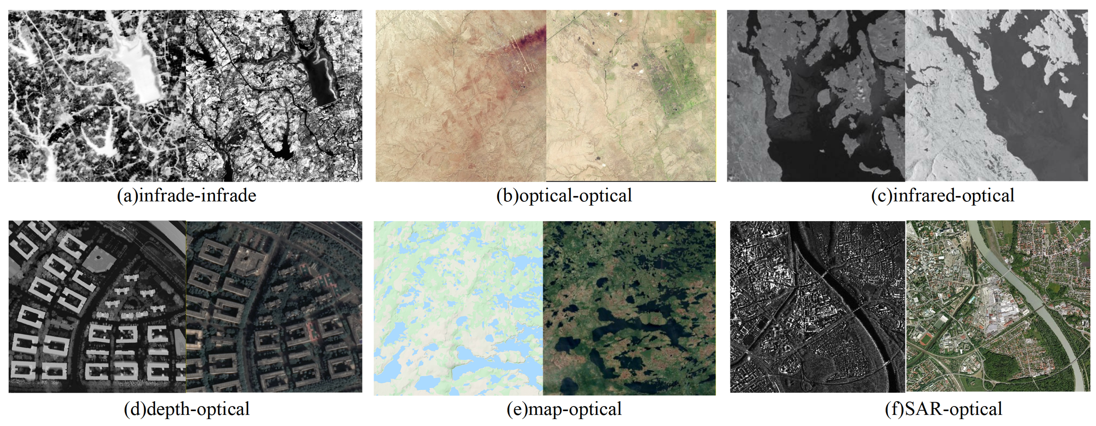
The evaluation utilizes a multimodal dataset comprising 60 image pairs, which are grouped into six distinct categories: infrared–infrared, optical–optical, infrared–optical, depth–optical, map–optical, and SAR–optical, with 10 pairs in each category. Representative examples are shown in Figure 4, and the source and scene information of each category are summarized in

Table 1. Summary of the multimodal datasets used in this study.

No.	Dataset Pair	Source and Scene
1	Infrared–Infrared	Self-constructed; mountainous river and reservoir regions; 30 m spatial resolution.
2	Optical–Optical	Source: https://github.com/LJY-RS/RIFT-multimodal-image-matching (accessed on 15 January 2026); dryland and semi-arid scenes.
3	Infrared–Optical	Source: https://github.com/LJY-RS/RIFT-multimodal-image-matching (accessed on 15 January 2026); coastal or inland waterbody scenes.
4	Depth–Optical	Source: https://github.com/LJY-RS/RIFT-multimodal-image-matching (accessed on 15 January 2026); urban residential scenes.
5	Map–Optical	Source: https://github.com/LJY-RS/RIFT-multimodal-image-matching (accessed on 15 January 2026); forest–lake and terrain scenes.
6	SAR–Optical	Source: https://github.com/LJY-RS/RIFT-multimodal-image-matching (accessed on 15 January 2026); urban scenes with rivers, roads, and man-made structures.

.

Among these categories, the infrared–infrared image pairs were constructed by ourselves, and all images in this subset have a spatial resolution of 30 m. The remaining five categories, namely optical–optical, infrared–optical, depth–optical, map–optical, and SAR–optical, were obtained from the RIFT multimodal image matching repository. For the five public subsets obtained from the RIFT repository, detailed sensor-level acquisition metadata, such as field of view, frame number, pixel pitch, and commercial camera model, were not provided in the original source. Therefore, in this study, we report the publicly available modality categories and scene characteristics of these subsets.

As shown in Figure 4, the six categories exhibit substantially different scene content and modality gaps. Figure 4a presents an infrared–infrared pair of mountainous river and reservoir regions, where the main difficulty arises from temporal variation and intensity change within the same modality. Figure 4b shows an optical–optical pair of dryland and semi-arid scenes, mainly affected by viewpoint variation and local geometric deformation. Figure 4c illustrates an infrared–optical pair of coastal or inland waterbody scenes, which exhibits a significant cross-modal radiometric gap. Figure 4d gives a depth–optical pair of urban residential regions, where the lack of rich texture in the depth image increases the difficulty of correspondence establishment. Figure 4e presents a map–optical pair of forest–lake and terrain scenes, characterized by a strong abstraction gap between symbolic map representation and natural optical appearance. Figure 4f shows a SAR–optical pair of urban scenes with rivers, roads, and dense man-made structures, where speckle noise and structural clutter introduce severe matching ambiguity.

Overall, the adopted benchmark covers six representative multimodal scenarios, including same-modality, cross-modality, symbolic-to-natural, and speckle-contaminated matching cases. These image pairs involve diverse remote sensing scenes, such as mountainous regions, water bodies, dryland surfaces, urban areas, and forested terrains, and exhibit evident nonlinear radiometric distortions, cross-modal appearance discrepancies, texture inconsistencies, and geometric deformations. Although the number of image pairs is limited, this benchmark still provides a challenging and diverse testbed for evaluating the robustness, stability, and geometric accuracy of multimodal matching methods. Following prior multimodal matching studies such as RIFT, we adopt this benchmark to enable direct and fair comparison with existing methods under widely recognized challenging conditions.

4.2. Qualitative Evaluation of Matching Results

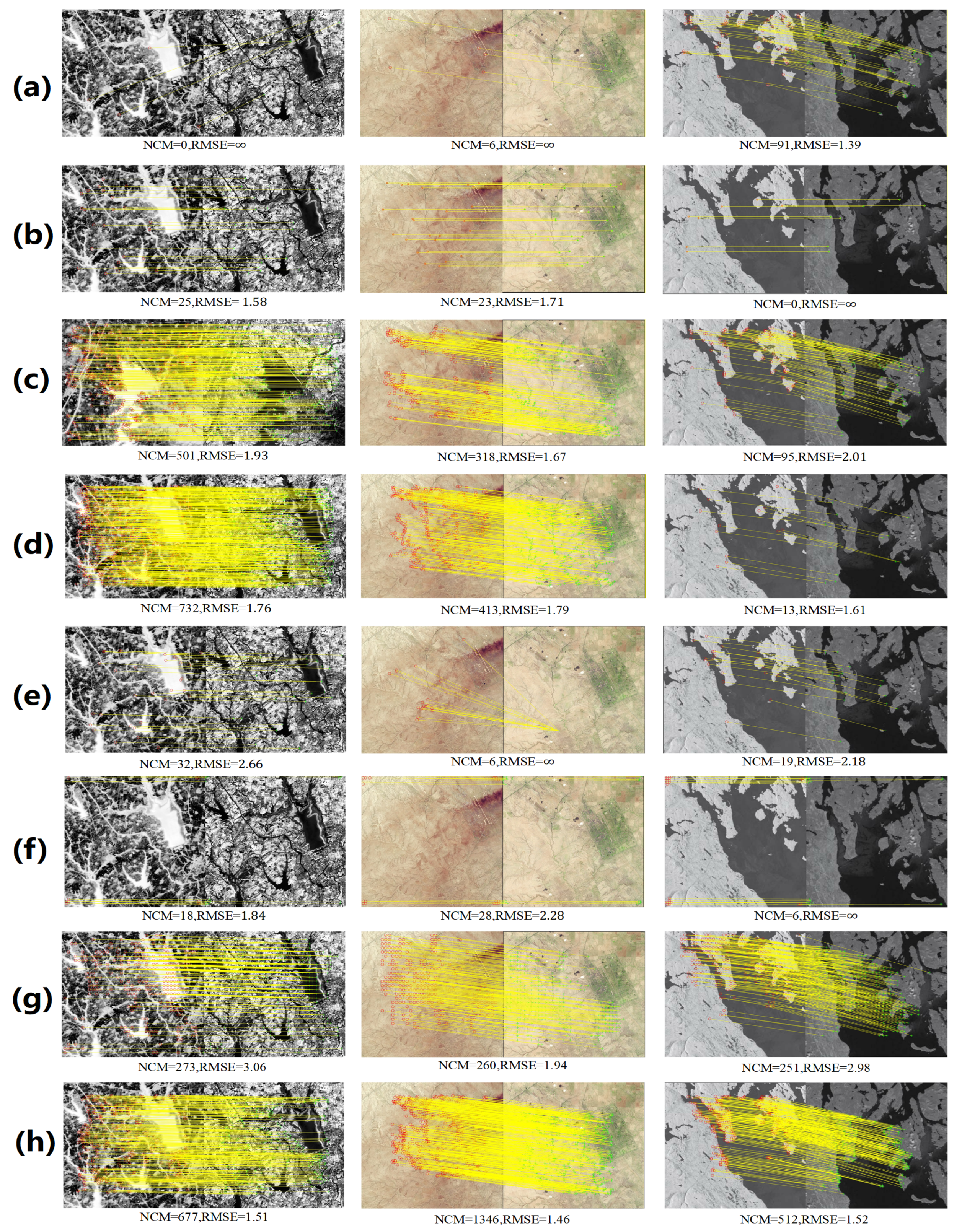
To intuitively demonstrate the robustness of the proposed SA-SWF under severe NRD and geometric deformation, representative image pairs from the six multimodal datasets were selected for qualitative visualization. Figure 5 presents the matching results for the infrared–infrared, optical–optical, and infrared–optical scenarios, which are mainly influenced by intensity variation and speckle-like interference. 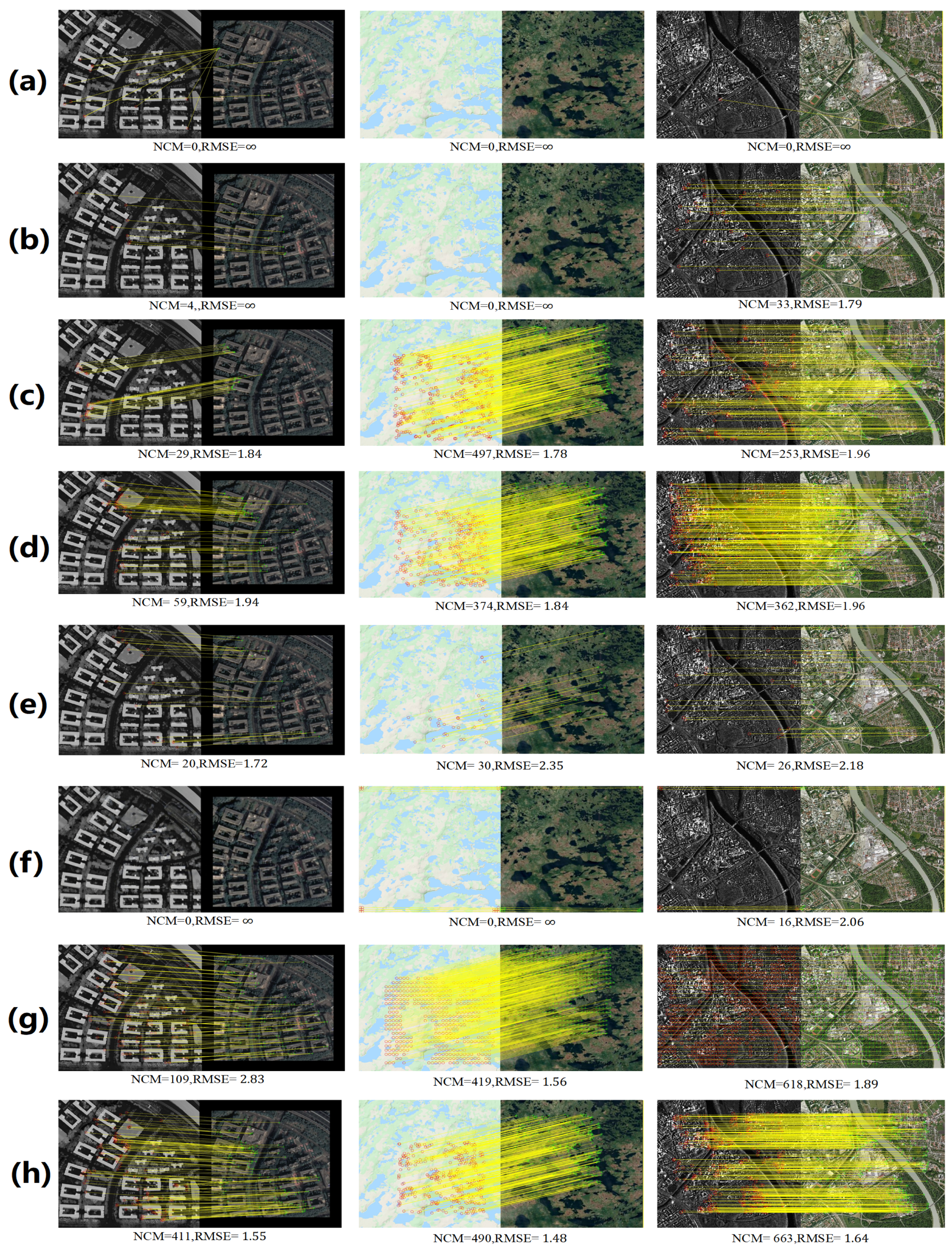Figure 6 further shows the results for three highly heterogeneous scenarios, namely depth–optical, map–optical, and SAR–optical. These examples represent particularly challenging matching conditions: the depth–optical pair involves texture-poor elevation data versus texture-rich optical imagery; the map–optical pair exhibits a large abstraction gap and rotation difference; and the SAR–optical pair is strongly affected by speckle noise and structural clutter.

The visualization results indicate that the proposed SA-SWF generally produces denser and more uniformly distributed correct correspondences, together with higher NCM and lower RMSE values in the representative examples, than the seven compared methods. As observed in both figures, gradient-based SIFT and correlation-based HOPC exhibit limited applicability under strong multimodal discrepancies. This limitation is reflected not only in the sparse distribution of yellow correspondence lines, but also in the low NCM values reported below the corresponding sub-images. For example, SIFT fails on most representative pairs, with RMSE = ∞ in five out of the six visualized cases, indicating that it is highly sensitive to strong radiometric inconsistency. Similarly, the deep learning-based methods do not always generalize well to these unseen modality combinations. CMM-Net yields sparse correspondences in difficult cases, such as NCM = 32 in the infrared–infrared scenario and NCM = 19 in the SAR–optical scenario. MatchFormer produces some valid matches, but they are often concentrated near image boundaries or local regions, as shown in Figure 5f, which leads to unstable registration geometry and relatively large RMSE values.

A more detailed comparison with phase-based and semantic methods further demonstrates the advantages of SA-SWF in balancing match quantity and geometric precision. In the depth–optical scenario shown in Figure 6 (left column), traditional phase-based methods are affected by the weak texture of the depth image. Although HAPCG yields 29 correct matches with an RMSE of 1.84 in the illustrated example, and RIFT produces 59 correct matches with an RMSE of 1.94, SA-SWF achieves 411 correct matches with a lower RMSE of 1.55. This result suggests that the proposed method can extract more reliable structural correspondences while maintaining high geometric accuracy. In the map–optical scenario in Figure 6 (middle column), the large rotation and abstraction gap degrade the performance of several competing methods. RIFT produces 374 correct matches but still suffers from an RMSE of 1.84, while SemLA achieves 419 correct matches with an RMSE of 1.56. In comparison, SA-SWF obtains 490 correct matches with a lower RMSE of 1.48, showing a better trade-off between correspondence density and registration precision. In the SAR–optical scenario in Figure 6 (right column), SA-SWF again achieves the most favorable overall result, with NCM = 663 and RMSE = 1.64, outperforming HAPCG (NCM = 253, RMSE = 1.96), RIFT (NCM = 362, RMSE = 1.96), and SemLA (NCM = 618, RMSE = 1.89). This comparison confirms the robustness of SA-SWF in the presence of severe speckle noise and complex urban structures.

Consistent observations can also be made from Figure 5. In the infrared–infrared scenario, SA-SWF produces dense and well-distributed correspondences with NCM = 677 and RMSE = 1.51, whereas methods such as CMM-Net and MatchFormer yield much fewer reliable matches. In the optical–optical scenario, SA-SWF achieves NCM = 1346 with RMSE = 1.46, which is noticeably better than the competing methods shown in the same column. In the infrared–optical scenario, where cross-modal radiometric discrepancy is particularly strong, SA-SWF still maintains high-quality correspondences with NCM = 512 and RMSE = 1.52, while several compared methods either generate sparse matches or suffer from larger registration errors.

In summary, the proposed SA-SWF consistently shows the most favorable qualitative performance in the representative examples. As shown in row (h) of Figure 5 and Figure 6, it generates dense, spatially well-distributed, and geometrically accurate correspondences, as reflected by the jointly favorable NCM and RMSE values reported below the sub-images. These results support the effectiveness of the proposed structure-aware descriptor and coarse-to-fine matching strategy in handling severe radiometric inconsistency and geometric deformation.

4.3. Quantitative Evaluation of Matching Results

The quantitative performance of the proposed SA-SWF method was evaluated against seven state-of-the-art baselines on the adopted multimodal benchmark comprising six representative dataset categories. The evaluation metrics, including the success rate (SR) and the number of correct matches (NCM), are summarized in

Table 2. Comparison of SR and Average NCM for Each Dataset. Bold values indicate the best performance.

Method	Multimodal Dataset Categories
	IR-IR		Opt-Opt		IR-Opt		Dpt-Opt		Map-Opt		SAR-Opt
	SR	NCM	SR	NCM	SR	NCM	SR	NCM	SR	NCM	SR	NCM
SIFT	0	0	60	18.4	30	20.2	10	3.8	0	0.4	0	0
HOPC	100	18.1	90	15.3	70	12.5	0	0.7	80	16.0	50	11.5
HAPCG	100	428.5	90	194.6	90	219.3	100	165.9	100	161.0	90	110.1
RIFT	100	479.9	90	195.4	90	159.3	100	145.6	90	115.2	60	84.6
CMM-Net	100	18.7	80	20.8	90	23.4	80	19.2	80	17.1	40	5.9
MatchFormer	100	18.3	100	22.7	100	21.8	100	23.1	90	18.2	70	14.6
SemLA	100	221.7	100	380.7	100	191.5	100	244.5	100	284.4	100	206.8
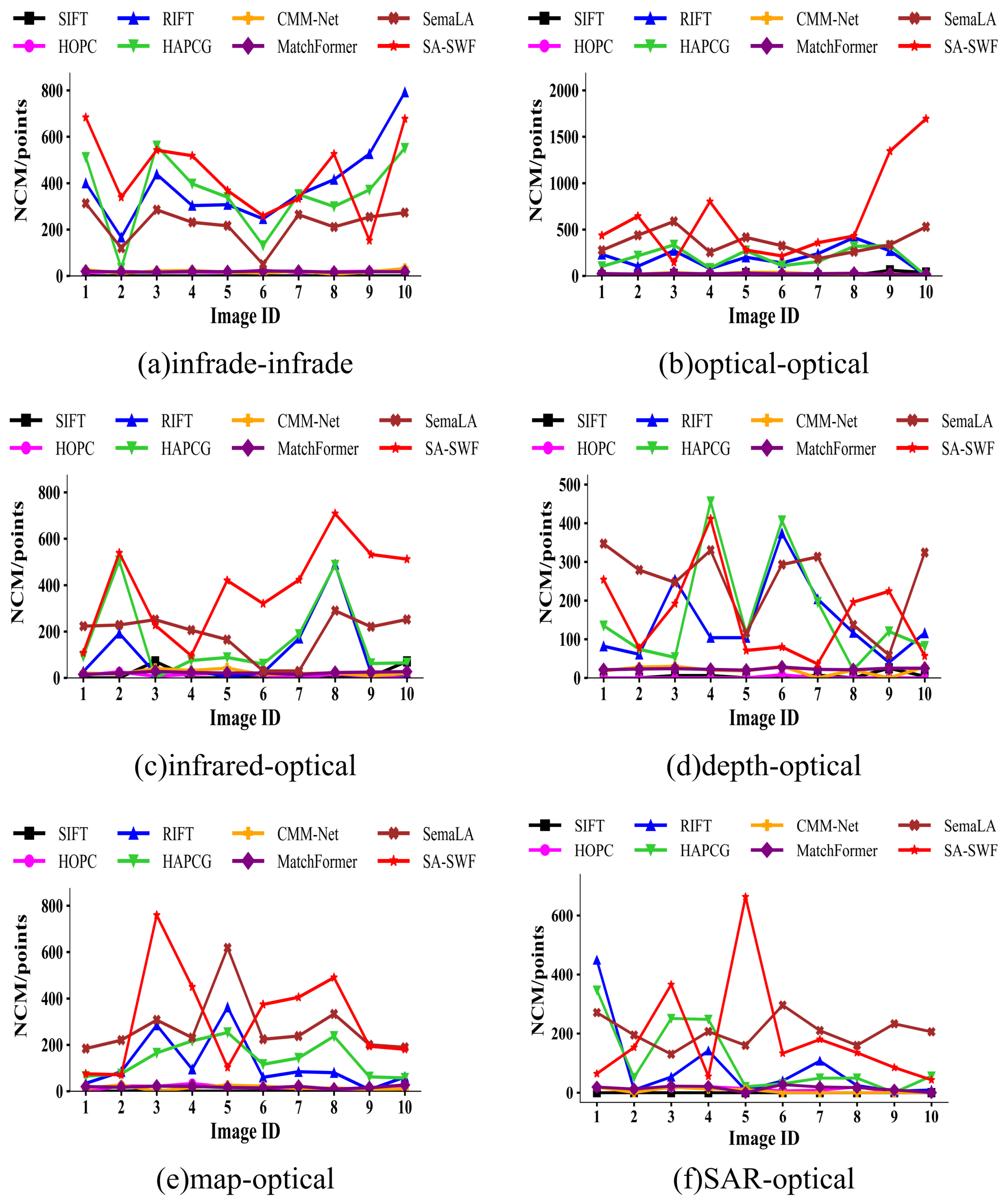
SA-SWF	100	439.7	100	634.7	100	388.5	100	159.8	100	310.2	100	207.7

, while the image-by-image NCM variation is illustrated in Figure 7. As shown in Figure 7, traditional methods such as SIFT and HOPC, as well as deep learning-based methods such as CMM-Net and MatchFormer, generally remain in the lower regions of the plots, indicating sparse correspondences and frequent matching failures. In contrast, the proposed SA-SWF, represented by the red curve, maintains a leading or competitive position across most dataset categories, demonstrating strong match abundance and overall stability on the adopted benchmark.

Specifically, in the optical–optical dataset shown in Figure 7b, SA-SWF achieves the highest average NCM of 634.7, which is substantially higher than SemLA (380.7) and HAPCG (194.6). A similar trend can be observed in the infrared–infrared dataset in Figure 7a, where SA-SWF achieves an average NCM of 439.7. Although RIFT attains a slightly higher average NCM of 479.9 in this category, the subsequent RMSE results show that SA-SWF provides better geometric precision and overall stability. In the infrared–optical dataset, SA-SWF again yields the best average NCM of 388.5, outperforming HAPCG (219.3), RIFT (159.3), and SemLA (191.5), which demonstrates its strong robustness under severe cross-modal radiometric discrepancy.

In the map–optical and SAR–optical datasets, SA-SWF also achieves the highest average NCM values, namely 310.2 and 207.7, respectively. In the depth–optical dataset, SA-SWF obtains an average NCM of 159.8, which is slightly lower than HAPCG (165.9) and SemLA (244.5). However, this difference in match quantity should be interpreted together with the RMSE results, because a larger number of correspondences does not necessarily imply higher geometric accuracy. Overall, SA-SWF achieves a 100% success rate across all six dataset categories, while maintaining the highest average NCM of 356.8 over the full benchmark, which indicates a favorable balance between correspondence quantity and reliability.

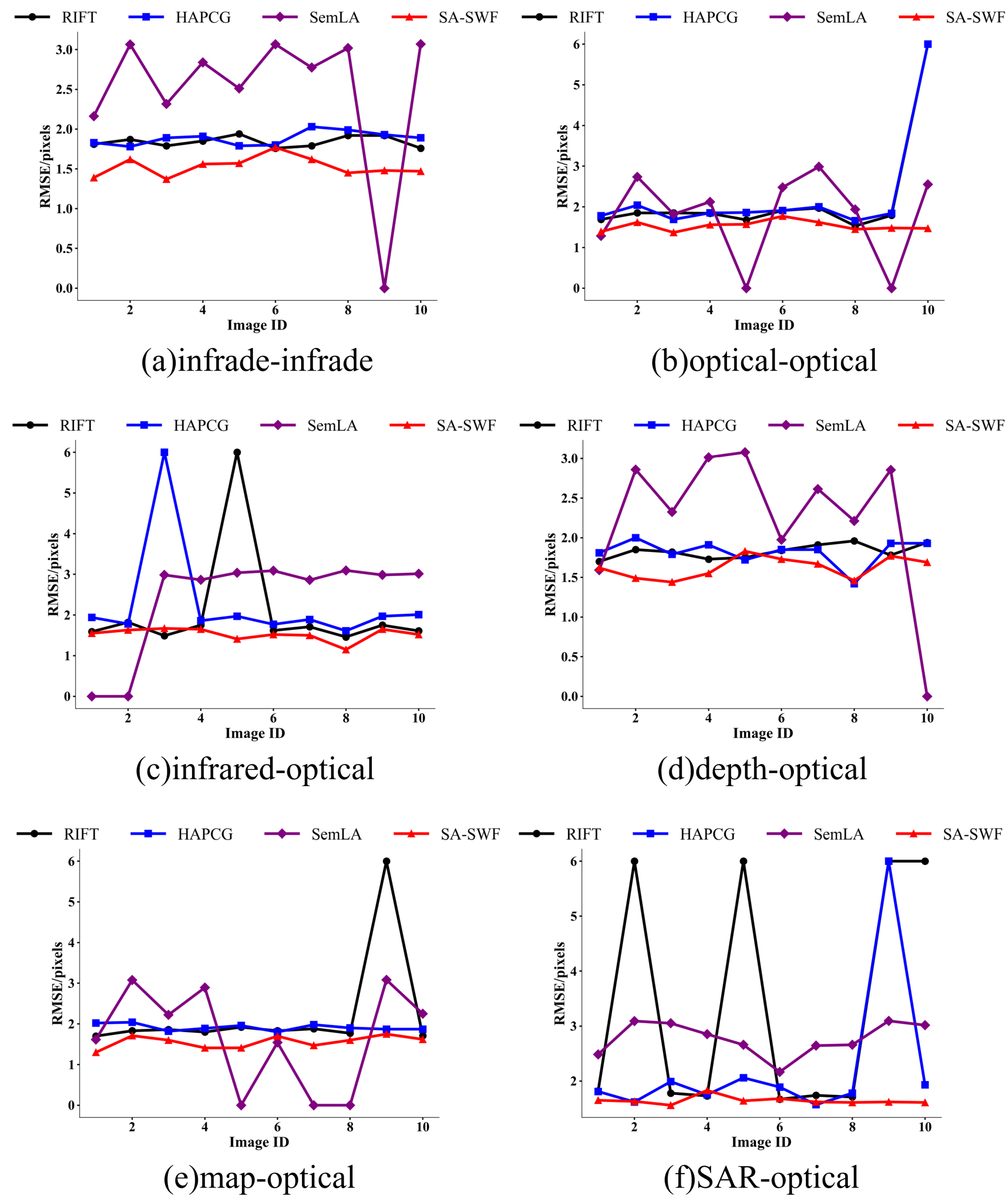
Geometric accuracy, quantified by the RMSE, is further summarized in

Table 3. Comparison of Average RMSE (Pixels) for Each Dataset. Bold values indicate the best performance.

Method	Average RMSE
	IR-IR	Opt-Opt	IR-Opt	Dpt-Opt	Map-Opt	SAR-Opt
SIFT	6.00	2.85	4.52	5.54	6.00	6.00
HOPC	1.57	1.85	2.92	6.00	2.40	3.81
HAPCG	1.88	2.26	2.28	1.82	1.91	2.24
RIFT	1.84	2.21	2.08	1.83	2.23	3.46
CMM-Net	2.19	2.93	2.62	3.01	2.65	4.40
MatchFormer	1.98	2.22	2.16	2.12	2.49	3.26
SemLA	2.48	1.79	2.39	2.25	1.67	2.77
SA-SWF	1.59	1.53	1.53	1.62	1.55	1.64

and visualized in Figure 8. While a high NCM is desirable, stability and geometric precision are more critical for practical multimodal registration. As shown in Figure 8, several competing methods exhibit considerable fluctuations across image pairs. For example, RIFT reaches an RMSE of 3.46 pixels in the SAR–optical dataset, while SemLA rises to 2.48 pixels in the infrared–infrared dataset. In contrast, the red curve corresponding to SA-SWF remains consistently low and relatively flat across all six categories.

This trend is quantitatively confirmed in Table 3, where SA-SWF is the only method that maintains an average RMSE below 1.65 pixels in every dataset category. Its average RMSE values range from 1.53 to 1.64 pixels, indicating strong geometric stability under different modality gaps and scene conditions. In particular, in the depth–optical dataset, SA-SWF achieves an RMSE of 1.62 pixels, outperforming HAPCG (1.82) and SemLA (2.25). Combined with the NCM results, this suggests that the correspondences produced by SA-SWF are not only sufficiently abundant, but also more structurally meaningful and accurately localized.

Although the benchmark size is limited, these quantitative comparisons remain informative because the adopted six-category benchmark covers substantially different modality gaps, scene structures, and deformation patterns, thereby enabling fair evaluation under representative multimodal matching conditions.

5. Discussion

Although the proposed method is built upon the edge-preserving property of the original side window filtering (SWF) method [27], the two methods differ substantially in both objective and methodological scope. The original SWF was proposed as an edge-aware local filtering technique, whose primary purpose is to suppress noise while preserving edges during image smoothing. In contrast, the proposed SA-SWF is a complete multimodal image matching framework specifically designed for robust correspondence establishment under nonlinear radiometric distortion, contrast inversion, weak texture, and geometric deformation. In the present work, SWF is extended from a basic filtering operator to a multi-scale anisotropic scale-space construction module, and is further integrated with multi-scale adaptive structure tensor detection, sub-pixel localization, structure-aware descriptor design, and coarse-to-fine geometric matching. These extensions allow the proposed framework not only to preserve structural edges, but also to extract repeatable keypoints, construct discriminative multimodal descriptors, and achieve accurate geometric alignment. The main differences between the original SWF and the proposed SA-SWF are summarized in

Table 4. Comparison between the original SWF and the proposed SA-SWF framework.

Aspect	Original SWF [27]	Proposed SA-SWF
Purpose	Edge-preserving image filtering	Complete multimodal matching framework
Core idea	Avoid edge blurring by side-window filtering	Extend SWF to multi-scale feature detection and multimodal matching
Scale space	Not designed for multimodal matching	Multi-scale anisotropic scale space for keypoint extraction
Detection	Not included	Adaptive structure tensor with grid constraint and sub-pixel refinement
Descriptor	Not included	SE-GLOH with gradient reversal invariance and entropy weighting
Matching	Not included	Coarse-to-fine matching with PCA and geometric verification
Multimodal robustness	Limited, since SWF is a filtering technique rather than a matching model	Designed for NRD, contrast inversion, weak texture, and geometric deformation
Output	Filtered image	Accurate correspondences and geometric alignment

.

To verify the specific contributions of the SWF-based multi-scale scale-space module and entropy-weighted attention (EWA) modules in multimodal alignment, we conducted an ablation study on two representative datasets: infrared–optical (IR-Opt) and SAR–optical (SAR-Opt). These two datasets were selected because they encapsulate the most significant challenges in multimodal registration: the IR-Opt pairs exhibit prevalent NRD and intensity inversions, while the SAR-Opt pairs are characterized by severe speckle noise and extreme geometric heterogeneity, providing a rigorous test for structural consistency and noise suppression. The quantitative results, summarized in

Table 5. Ablation Study of Core Modules on IR-Opt and SAR-Opt Datasets. Bold and gray background indicate the best performance of our full model. ↑ indicates higher is better, and ↓ indicates lower is better.

Experiment	Infrared-Optical		SAR-Optical
	NCM ↑	RMSE ↓	NCM ↑	RMSE ↓
No_Entropy	237.6	1.79	81.6	1.81
No_SWF	263.6	1.71	94.8	1.80
SA-SWF (Full)	388.5	1.53	183.8	1.62

, demonstrate that both modules are indispensable for achieving high-precision alignment.

As indicated by the quantitative data, the EWA module plays a decisive role in enhancing descriptor discriminativeness. In the IR-Opt scenario, removing the EWA module (No_Entropy) causes NCM to drop from 388.5 to 237.6, while the average RMSE degrades significantly from 1.53 to 1.79 pixels. This performance gap is even more pronounced in the SAR-Opt dataset, where the NCM plummet from 183.8 to 81.6. These results indicate that the entropy-weighted mechanism effectively identifies and prioritizes informative geometric structures by evaluating local structural uncertainty. By modulating the gradient response with a soft attention mask, the descriptor successfully suppresses pseudo-matches in textureless or noisy regions, thereby ensuring high geometric fidelity even at the cost of excluding low-confidence candidates.

Furthermore, the contribution of the SWF module is validated by its impact on keypoint localization consistency. Without SWF (No_SWF), the algorithm relies on conventional filtering for scale-space construction, which leads to an RMSE increase across both datasets (from 1.53 to 1.71 in IR-Opt and from 1.62 to 1.80 in SAR-Opt). This confirms that SWF is essential for maintaining the positional integrity of keypoints across multimodal scales. By preserving salient structural edges during the smoothing process, SWF avoids the edge-shifting problems inherent in traditional Gaussian filters, providing a more stable foundation for the subsequent matching stage. Ultimately, the full SA-SWF model achieves the optimal balance of match density and precision, proving that the synergy between structural edge preservation and entropy-based attention is the key to surmounting extreme radiometric and geometric distortions.

6. Conclusions

In this paper, we propose a novel multimodal image matching framework entitled structure-aware feature descriptor with multi-scale side window filtering (SA-SWF). The proposed method effectively integrates anisotropic side window filtering, multi-scale adaptive structure tensor detection, gradient reversal invariance, entropy-weighted attention, and coarse-to-fine geometric refinement into a unified matching pipeline. Through this design, SA-SWF is able to preserve salient structural edges during scale-space construction, extract highly repeatable keypoints with sub-pixel localization accuracy, and build discriminative descriptors that remain robust under severe nonlinear radiometric distortion (NRD), contrast inversion, weak texture, and geometric deformation. Experimental evaluation on 60 multimodal remote sensing image pairs from six categories, including infrared–infrared, optical–optical, infrared–optical, depth–optical, map–optical, and SAR–optical datasets, demonstrates the superior performance of the proposed method. Compared with seven state-of-the-art baselines, namely SIFT, HOPC, HAPCG, RIFT, CMM-Net, MatchFormer, and SemLA, SA-SWF consistently achieves the best overall results. Across all six dataset categories, SA-SWF attains a 100% success rate, the highest average number of correct matches (356.8), and the lowest average root mean square error (1.57 pixels). These results confirm that the proposed framework provides excellent robustness, stability, and geometric accuracy under extreme radiometric and geometric distortions. Despite these advantages, SA-SWF still has a relatively high computational cost because of the multi-scale filtering process, entropy-guided descriptor construction, and subsequent geometric refinement. In future work, we will focus on improving computational efficiency through accelerated implementation and lightweight optimization, and on further expanding the benchmark dataset to validate the method under more diverse multimodal imaging conditions and larger-scale application scenarios.

References

- Senthilnath, J.; Omkar, S.; Mani, V.; Karthikeyan, T. Multiobjective discrete particle swarm optimization for multisensor image alignment. IEEE Geosci. Remote Sens. Lett. 2013, 10, 1095–1099. [Google Scholar] [CrossRef] [Scilit]
- Ye, Y.; Bruzzone, L.; Shan, J.; Bovolo, F.; Zhu, Q. Fast and robust matching for multimodal remote sensing image registration. IEEE Trans. Geosci. Remote Sens. 2019, 57, 9059–9070. [Google Scholar] [CrossRef] [Scilit]
- Jiang, X.; Ma, J.; Xiao, G.; Shao, Z.; Guo, X. A review of multimodal image matching: Methods and applications. Inf. Fusion 2021, 73, 22–71. [Google Scholar] [CrossRef] [Scilit]
- Yao, Y.; Zhang, Y.; Wan, Y.; Liu, X.; Yan, X.; Li, J. Multi-modal remote sensing image matching considering co-occurrence filter. IEEE Trans. Image Process. 2022, 31, 2584–2597. [Google Scholar] [CrossRef] [Scilit] [PubMed]
- Yoo, J.C.; Han, T.H. Fast normalized cross-correlation. Circuits Syst. Signal Process. 2009, 28, 819–843. [Google Scholar] [CrossRef] [Scilit]
- Suri, S.; Reinartz, P. Mutual-information-based registration of TerraSAR-X and Ikonos imagery in urban areas. IEEE Trans. Geosci. Remote Sens. 2009, 48, 939–949. [Google Scholar] [CrossRef] [Scilit]
- Maes, F.; Collignon, A.; Vandermeulen, D.; Marchal, G.; Suetens, P. Multimodality image registration by maximization of mutual information. IEEE Trans. Med. Imaging 2002, 16, 187–198. [Google Scholar] [CrossRef] [Scilit]
- Viola, P.; Wells, W.M., III. Alignment by maximization of mutual information. Int. J. Comput. Vis. 1997, 24, 137–154. [Google Scholar] [CrossRef] [Scilit]
- Ye, Y.; Shen, L. Hopc: A novel similarity metric based on geometric structural properties for multi-modal remote sensing image matching. ISPRS Ann. Photogramm. Remote Sens. Spat. Inf. Sci. 2016, 3, 9–16. [Google Scholar] [CrossRef] [Scilit]
- Lowe, D.G. Distinctive image features from scale-invariant keypoints. Int. J. Comput. Vis. 2004, 60, 91–110. [Google Scholar] [CrossRef] [Scilit]
- Ma, W.; Wen, Z.; Wu, Y.; Jiao, L.; Gong, M.; Zheng, Y.; Liu, L. Remote sensing image registration with modified SIFT and enhanced feature matching. IEEE Geosci. Remote Sens. Lett. 2016, 14, 3–7. [Google Scholar] [CrossRef] [Scilit]
- Morel, J.M.; Yu, G. ASIFT: A new framework for fully affine invariant image comparison. SIAM J. Imaging Sci. 2009, 2, 438–469. [Google Scholar] [CrossRef] [Scilit]
- Li, J.; Hu, Q.; Ai, M. RIFT: Multi-modal image matching based on radiation-variation insensitive feature transform. IEEE Trans. Image Process. 2019, 29, 3296–3310. [Google Scholar] [CrossRef] [Scilit] [PubMed]
- Aguilera, C.A.; Sappa, A.D.; Toledo, R. LGHD: A feature descriptor for matching across non-linear intensity variations. In 2015 IEEE International Conference on Image Processing (ICIP); IEEE: New York, NY, USA, 2015; pp. 178–181. [Google Scholar] [CrossRef] [Scilit]
- Zhang, Y.; Yao, Y.; Wan, Y.; Liu, W.; Yang, W.; Zheng, Z.; Xiao, R. Histogram of the orientation of the weighted phase descriptor for multi-modal remote sensing image matching. ISPRS J. Photogramm. Remote Sens. 2023, 196, 1–15. [Google Scholar] [CrossRef] [Scilit]
- Serrano, D.; Szymkowiak, J.; Musialski, P. HOSC: A periodic activation function for preserving sharp features in implicit neural representations. arXiv 2024, arXiv:2401.10967. [Google Scholar] [CrossRef] [Scilit]
- Yao, Y.; Zhang, Y.; Wan, Y.; Liu, X.; Guo, H. Heterologous Image Matching Considering Anisotropic Weighted Moment and Absolute Phase Orientation. Geomat. Inf. Sci. Wuhan Univ. 2021, 46, 1727–1736. (In Chinese) [Google Scholar] [CrossRef]
- Yu, W.; Sun, X.; Yang, K.; Rui, Y.; Yao, H. Hierarchical semantic image matching using CNN feature pyramid. Comput. Vis. Image Underst. 2018, 169, 40–51. [Google Scholar] [CrossRef] [Scilit]
- Ma, L.; Lu, Z.; Shang, L.; Li, H. Multimodal convolutional neural networks for matching image and sentence. In 2015 IEEE International Conference on Computer Vision (ICCV); IEEE: New York, NY, USA, 2015; pp. 2623–2631. [Google Scholar] [CrossRef] [Scilit]
- Quan, D.; Wang, S.; Li, Y.; Yang, B.; Huyan, N.; Chanussot, J.; Hou, B.; Jiao, L. Multi-relation attention network for image patch matching. IEEE Trans. Image Process. 2021, 30, 7127–7142. [Google Scholar] [CrossRef] [Scilit]
- Li, L.; Liu, M.; Ma, L.; Han, L. Cross-Modal feature description for remote sensing image matching. Int. J. Appl. Earth Obs. Geoinf. 2022, 112, 102964. [Google Scholar] [CrossRef] [Scilit]
- Wang, Q.; Zhang, J.; Yang, K.; Peng, K.; Stiefelhagen, R. Matchformer: Interleaving attention in transformers for feature matching. In Proceedings of the Asian Conference on Computer Vision, Macau, China, 4–8 December 2022; pp. 2746–2762. [Google Scholar] [CrossRef] [Scilit]
- Xie, H.; Zhang, Y.; Qiu, J.; Zhai, X.; Liu, X.; Yang, Y.; Zhao, S.; Luo, Y.; Zhong, J. Semantics lead all: Towards unified image registration and fusion from a semantic perspective. Inf. Fusion 2023, 98, 101835. [Google Scholar] [CrossRef] [Scilit]
- Xu, W.; Yuan, X.; Hu, Q.; Li, J. SAR-optical feature matching: A large-scale patch dataset and a deep local descriptor. Int. J. Appl. Earth Obs. Geoinf. 2023, 122, 103433. [Google Scholar] [CrossRef] [Scilit]
- Lan, C.; Lu, W.; Yu, J.; Xu, Q. Deep Learning Algorithms for Feature Matching of Heterogeneous Remote Sensing Images. Acta Geod. Cartogr. Sin. 2021, 50, 189–202. (In Chinese) [Google Scholar] [CrossRef]
- Yang, B.; Song, W.; Jin, H.; Li, S. Infrared Small Target Detection Based on Gradient-Difference Anisotropic Gaussian Filtering. Laser Optoelectron. Prog. 2023, 60, 1612003. (In Chinese) [Google Scholar] [CrossRef] [Scilit]
- Yin, H.; Gong, Y.; Qiu, G. Side window filtering. In 2019 IEEE/CVF Conference on Computer Vision and Pattern Recognition (CVPR); IEEE: New York, NY, USA, 2019; pp. 8758–8766. [Google Scholar] [CrossRef] [Scilit]
- Dalal, N.; Triggs, B. Histograms of oriented gradients for human detection. In CVPR ’05:Proceedings of the 2005 IEEE Computer Society Conference on Computer Vision and Pattern Recognition (CVPR’05); IEEE: New York, NY, USA, 2005; Volume 1, pp. 886–893. [Google Scholar] [CrossRef] [Scilit]
- Mikolajczyk, K.; Schmid, C. A performance evaluation of local descriptors. IEEE Trans. Pattern Anal. Mach. Intell. 2005, 27, 1615–1630. [Google Scholar] [CrossRef] [Scilit] [PubMed]
- Zhao, Z.; Wang, F.; You, H. Robust region feature extraction with salient mser and segment distance-weighted gloh for remote sensing image registration. IEEE J. Sel. Top. Appl. Earth Obs. Remote Sens. 2023, 17, 2475–2488. [Google Scholar] [CrossRef] [Scilit]
- Ye, Y.; Shan, J.; Bruzzone, L.; Shen, L. Robust registration of multimodal remote sensing images based on structural similarity. IEEE Trans. Geosci. Remote Sens. 2017, 55, 2941–2958. [Google Scholar] [CrossRef] [Scilit]
- Fan, J.; Xiong, Q.; Ye, Y.; Li, J. Combining phase congruency and self-similarity features for multimodal remote sensing image matching. IEEE Geosci. Remote Sens. Lett. 2023, 20, 4001105. [Google Scholar] [CrossRef] [Scilit]
- Xia, C.; Li, X.; Zhao, L.; Shu, R. Infrared small target detection based on multiscale local contrast measure using local energy factor. IEEE Geosci. Remote Sens. Lett. 2019, 17, 157–161. [Google Scholar] [CrossRef] [Scilit]
- Bansal, M.; Kumar, M.; Kumar, M.; Kumar, K. An efficient technique for object recognition using Shi-Tomasi corner detection algorithm. Soft Comput. 2021, 25, 4423–4432. [Google Scholar] [CrossRef] [Scilit]
- Loog, M.; Lauze, F. The improbability of Harris interest points. IEEE Trans. Pattern Anal. Mach. Intell. 2010, 32, 1141–1147. [Google Scholar] [CrossRef] [Scilit] [PubMed]
- Fischler, M.A.; Bolles, R.C. Random sample consensus: A paradigm for model fitting with applications to image analysis and automated cartography. Commun. ACM 1981, 24, 381–395. [Google Scholar] [CrossRef] [Scilit]
- Hartley, R.; Zisserman, A. Multiple View Geometry in Computer Vision; Cambridge University Press: Cambridge, UK, 2003. [Google Scholar] [CrossRef] [Scilit]
- Li, J.; Xu, W.; Shi, P.; Zhang, Y.; Hu, Q. LNIFT: Locally normalized image for rotation invariant multimodal feature matching. IEEE Trans. Geosci. Remote Sens. 2022, 60, 5621314. [Google Scholar] [CrossRef] [Scilit]