Cross-Dataset Benchmarking of Deep Learning Models for Surface Defect Classification in Metal Parts

Abstract

Accurate surface defect classification is critical for industrial quality control. Although Deep Learning achieves strong results on individual datasets, most prior studies benchmark only a narrow set of models under inconsistent pipelines, limiting comparability and industrial relevance. This work introduces the first systematic benchmark of ten architectures—CNNs (CNN, ResNet18/50), lightweight models (MobileNetV2, SuperSimpleNet, GhostNet, EfficientNetV2), Vision Transformers (Swin Transformer), a hybrid CNN–Transformer (CoAtNet), and a one-stage detector (YOLOv12)—across five public defect datasets (NEU-DET, X-SDD, KolektorSDD2, DAGM, MTDD) under a unified pipeline. Results show that Swin Transformer and CoAtNet achieve the best performance (mean F1-scores 90.8% and 85.5%), while EfficientNetV2 underperformed (41.9%), underscoring the need for domain-specific benchmarks. Lightweight models such as MobileNetV2, GhostNet, and SuperSimpleNet deliver competitive accuracy at much lower cost, offering practical solutions for edge deployment. By bridging the gap between academic benchmarks and manufacturing requirements, this study provides actionable guidance for selecting defect detection models in automated inspection.

1. Introduction

Quality inspection of steel and metallic surfaces is a critical step in modern manufacturing, directly influencing the performance, reliability, and market value of final products. Surface defects such as scratches, cracks, inclusions, and pits can compromise structural integrity, cause premature failure, and lead to costly material rejection. Traditionally, visual inspection has been the primary method for detecting and classifying such defects. However, it is labor-intensive, prone to subjectivity, and often inconsistent.

The emergence of Deep Learning (DL) and Computer Vision has transformed industrial inspection, offering automated systems capable of classifying surface defects with high accuracy and reproducibility. Convolutional Neural Networks (CNNs) and their variants have achieved remarkable success in classification tasks, while more recent architectures such as Vision Transformers (ViTs), lightweight CNNs, and hybrid CNN–Transformer models are pushing the boundaries of scalability and deployment efficiency. Despite these advances, the literature remains fragmented: most studies focus on a small subset of models, evaluate them on limited datasets, or adopt inconsistent training and testing protocols, which prevents fair and comprehensive comparisons. This article addresses this gap by presenting the first systematic benchmark that evaluates ten diverse deep learning architectures—ranging from classical CNNs (CNN, ResNet18/50), lightweight models (MobileNetV2, SuperSimpleNet, GhostNet, EfficientNetV2), Vision Transformers (Swin Transformer), hybrid CNN–Transformer networks (CoAtNet), and one-stage detectors (YOLOv12)—across five widely used surface defect datasets (NEU-DET, X-SDD, KolektorSDD2, DAGM, MTDD). All models were trained under a unified pipeline and assessed with standard metrics (accuracy, precision, recall, F1-score) alongside training and execution time, ensuring a fair, cross-architecture comparison. This study not only quantifies performance but also highlights the trade-offs between accuracy, computational efficiency, and suitability for real-world deployment on industrial inspection lines.

The contributions of this work are:

• Provide the first large-scale, multi-architecture, and multi-dataset benchmark for surface defect classification, enabling consistent comparison across CNNs, lightweight networks, transformers, and hybrid models.
• Evaluate models not only in terms of accuracy but also in terms of efficiency and training cost, offering insights into deployment trade-offs critical for real-time or edge applications.
• Demonstrate which architectures generalize best across diverse datasets, bridging the gap between research-oriented accuracy and the practical requirements of industrial feasibility.

2. Related Work

Machine Learning (ML)-based approaches have achieved great performance in object classification tasks within Computer Vision scope. However, traditional ML methods typically depend on explicit feature extraction, often requiring domain-specific knowledge, manual intervention, and expertise from the user, which limits scalability and adaptability in complex industrial contexts. In contrast, DL, a specialized branch of ML characterized by large neural network architectures, enables automatic feature extraction directly from raw data. This eliminates the need for handcrafted features while offering enhanced scalability, improved generalization across diverse datasets, and greater adaptability to complex visual tasks compared to conventional ML pipelines. Given these advantages, deep learning has become a leading paradigm for visual inspection tasks, including defect classification in manufacturing, particularly when the target defect categories are known in advance and sufficient labelled data are available.

This section specifically investigates the generalization performance of selected DL methods across multiple benchmark datasets for defect-type classification. Accordingly, the review focuses exclusively on related work employing DL algorithms, with particular attention to convolutional networks, transformers, and hybrid architectures relevant to industrial inspection scenarios.

CNN-Based Classification Methods have been widely applied to steel surface defect classification. CNNs are characterized by stacked convolutional and pooling layers that automatically extract hierarchical features, progressing from low-level edges and textures to high-level semantic patterns. This architecture leverages weight sharing and local receptive fields, making CNNs both computationally efficient and effective in capturing spatially localized defect characteristics. For classification tasks, the extracted feature maps are typically passed through fully connected layers or global pooling operations, producing class predictions that reflect the presence of specific defect types. Feng et al. [1] fused a ResNet50 backbone with an FcaNet channel-attention and a CBAM spatial-attention module, achieving 94.1% classification accuracy on a strip-steel defect dataset (X-SDD). Chan et al. [2] proposed FOHR-Net, a feature-optimization network that combines multi-layer feature alignment and dual-branch recombination modules. Evaluated on several defect datasets (NEU-DET, GC10-DET, APDDD), FOHR-Net achieved a mean Average Precision (mAP) of 78.3% on the NEU-DET dataset, outperforming standard detectors. Recent CNN variants frequently utilize ResNet and similar encoders to extract deep features, often incorporating attention mechanisms or feature-fusion enhancements to improve performance and convergence. For example, replacing conventional convolutional blocks with Ghost modules and integrating attention mechanisms into a YOLOv8 backbone improved detection performance on steel surface defect datasets, highlighting the advantages of lightweight CNN design [3].

U-Net and related encoder–decoder architectures are commonly used for pixel-wise defect segmentation. These architectures extend the CNN design by combining a contracting encoder path, which captures hierarchical features, with a symmetric decoder path that progressively upsamples and refines spatial details. Skip connections are employed to fuse fine-grained information from earlier layers with deeper feature maps, improving localization accuracy in segmentation tasks. Konovalenko et al. [4] evaluated several U-Net variants on metal strip images and reported that a U-Net with a ResNet-152 encoder achieved the highest segmentation accuracy compared to other 13 models, including MobileNet and EfficientNet. Similarly, Liu et al. [5] introduced the MSDD-UNet, incorporating multi-scale dense blocks for scratch detection. On the NEU-Seg dataset, MSDD-UNet achieved the highest Intersection over Union (IoU) among the methods tested, outperforming standard U-Net and U-Net++. Specifically, MSDD-UNet improved IoU by 4.98% over the DeepLabv3+ (MobileNetV2) baseline. These results demonstrate that utilizing deeper encoders, dilated convolutions, or attention mechanisms in U-Net-based architectures can significantly improve defect mask segmentation as measured by IoU and Dice Similarity Coefficient (DSC).

Autoencoder and Anomaly Detection Approaches have been applied for anomaly-based defect detection. An autoencoder consists of two main components: an encoder that compresses the input into a lower-dimensional latent representation, and a decoder that reconstructs the input from this latent space. When trained only on defect-free images, the network learns the normal texture distribution, and reconstruction errors emerge when it encounters unseen or anomalous patterns. This reconstruction-error principle enables the detection of defects without explicitly training on defective samples, making autoencoders particularly effective in situations with limited or imbalanced defect data. Tesfaye et al. [6] employed a two-stage convolutional autoencoder incorporating an artificial-defect generation step during training. Their method achieved state-of-the-art detection performance, attaining an average Area Under the ROC Curve (AUROC) of 97.7% across six object classes in the MVTec anomaly detection dataset. Such approaches are particularly relevant for industrial inspection scenarios where collecting large, balanced datasets of all defect types is challenging; by focusing only on defect-free samples, anomaly detection methods provide a practical alternative for rare or previously unseen defects, complementing supervised classification approaches.

Vision Transformers (ViTs) are based on the Transformer architecture, initially introduced in 2017 [7]. In ViTs, an input image is divided into fixed-size linearly embedded patches and treated as a sequence, similar to word tokens in natural language processing. These patch embeddings are processed through layers of multi-head self-attention and feed-forward networks, enabling the model to capture local and global dependencies. Unlike convolutional networks, which rely on hierarchical receptive fields, ViTs learn relationships between all patches in parallel, providing strong scalability to large datasets and high-resolution images. Recent surface-inspection studies have adapted attention-based mechanisms under the assumption that industrial defects often require global context modelling, multi-scale feature extraction, and selective emphasis on subtle defect regions embedded in noisy or repetitive textures. Wei et al. [8] proposed RFAConv-CBM-ViT, an enhanced ViT architecture that integrates a Receptive-Field Attention Convolution (RFAConv) module and a Context-Broadcasting Median (CBM) mechanism. The RFAConv module adaptively adjusts the receptive field of patch embeddings to capture multi-scale defect features. At the same time, the CBM mechanism merges median representations in the Multilayer Perceptron (MLP) to suppress noise. According to the authors, RFAConv-CBM-ViT demonstrated consistent performance across various metal surface defect datasets by improving global feature extraction without introducing additional computational overhead or increasing model complexity. ViT-based approaches are particularly promising for this work because their self-attention mechanism excels at modeling long-range dependencies and capturing global context, essential for identifying subtle or spatially distributed surface defects that purely convolutional models may overlook.

One-Stage Object Detectors, particularly the You Only Look Once (YOLO) family, are widely used for real-time defect detection. Unlike two-stage detectors that first generate region proposals, YOLO directly predicts bounding boxes and class probabilities in a single forward pass over the image, which makes it extremely fast. The architecture typically consists of a backbone for feature extraction, a neck (e.g., FPN or PAN) for multi-scale feature fusion, and a head that outputs bounding box coordinates, objectness scores, and class predictions. This unified design minimizes computational overhead while maintaining competitive accuracy, enabling YOLO models to achieve high inference speeds suitable for real-time inspection. Liu et al. [9] introduced SLF-YOLO, a lightweight YOLOv8-based model incorporating novel SC_C2f gated modules and a Light-SSF neck to enhance multi-scale feature fusion. SLF-YOLO also employs a fine-grained “FI-Metal-IoU” loss function to improve the localization of minor defects. On the NEU-DET steel surface dataset, SLF-YOLO achieved 80.0% mAP, outperforming the baseline YOLOv8 (75.9% mAP), and reached 86.8% mAP on the AL10-DET dataset. These results indicate that targeted modifications to YOLO backbones can substantially improve detection precision on metallic defects. Similarly, Ma et al. [3] replaced the standard YOLOv8 convolutions with Ghost modules and integrated a multi-scale positional attention mechanism. Their model achieved a processing speed of 171.5 FPS on NEU-DET while maintaining a mAP of 78.6%. Recent YOLO variants can perform real-time NEU-type defect detection with mAP scores in the high 70s to low 80s. Such one-stage detectors are highly relevant to this work because they combine competitive accuracy with high inference speed. They are well-suited for deployment in industrial inspection lines where defects must be detected and classified continuously in real time.

Faster R-CNN and Two-Stage Detectors are frequently applied for more precise defect localization. The Faster R-CNN architecture consists of three main components: (i) a convolutional backbone for feature extraction, (ii) a Region Proposal Network (RPN) that generates candidate object regions, and (iii) a region-of-interest pooling stage followed by fully connected layers for classification and bounding box regression. This two-stage design allows the network to focus on likely defect areas and refine its classification and localization, making it more accurate than single-stage detectors, albeit typically slower. Taewook et al. [10] proposed D²;-SPDM, a framework that initially applies Faster R-CNN (with ResNet-50, Inception-V2, or VGG-16 backbones) for defect bounding box detection, followed by segmentation refinement using GrabCut and DeepLabV3+. The ResNet-50 version of their framework attained the highest mAP of 76.6% on the NEU-DET dataset. Their analysis demonstrated that Faster R-CNN (ResNet-50) outperforms single-stage SSD and YOLOv4 models in accuracy, albeit at lower frames per second (FPS). Such two-stage detectors are particularly relevant because their region proposal mechanisms and refinement stages enable finer localization of small or subtle surface defects. This is critical in applications where detection precision takes priority over inference speed.

In summary, DL approaches for metal surface defect detection and classification have advanced considerably over the past five years. CNNs enhanced with attention mechanisms (e.g., ResNet with Ghost modules) and segmentation architectures such as U-Net consistently achieve high classification accuracy and precise mask predictions on benchmark datasets [1,5]. Object detectors, including YOLO and Faster R-CNN, further enable localized defect detection, typically reporting mAP scores in the range of 75–80% on widely used steel surface datasets [9,10]. Alternative paradigms such as ViTs and unsupervised autoencoders have recently shown competitive results across diverse data sources. Collectively, works published between 2020 and 2025 demonstrate that state-of-the-art neural networks can deliver strong performance in detecting subtle and heterogeneous surface defects. When incorporating architectural adaptations such as attention or feature fusion, or task-specific loss functions like IoU-based losses [2,9]. These Neural Networks outperform classical techniques.

Despite these advances, several gaps remain. Existing studies typically evaluate only a narrow set of architectures [11,12] and rely on heterogeneous pre-processing steps or evaluation protocols, making cross-study comparisons unreliable. Furthermore, computational trade-offs between accuracy, efficiency, and training and execution time are rarely discussed, despite these aspects being crucial for real-world deployment on manufacturing lines, where edge devices require both real-time inference and resource efficiency.

These limitations motivate the present study. Unlike prior efforts, this study provides the first comprehensive benchmark of ten diverse deep learning models—including CNN baselines, lightweight architectures (MobileNetV2, SuperSimpleNet, GhostNet, EfficientNetV2), deeper residual networks (ResNet18, ResNet50), ViTs (Swin Transformer), hybrid CNN–Transformer designs (CoAtNet), and a modern one-stage detector (YOLOv12)—evaluated across five widely used surface defect datasets: NEU-DET, X-SDD, KolektorSDD2, DAGM, MTDD.

By training and testing all models under a unified pipeline and standardized metrics (accuracy, precision, recall, F1-score, training and execution time), this study delivers the first systematic, cross-architecture comparison in this field. In doing so, it contributes novel and actionable insights into the trade-offs between accuracy, computational complexity, and inference speed. Thus, directly supports the transition from research-driven performance claims to practical, industry-grade surface defect detection systems deployment.

The remainder of this article is organized as follows. Section 3 describes the methodology, including the model architectures, datasets, training setup, and evaluation metrics. Section 4 presents the experimental findings, reporting classification performance, training times, and inference latencies. Section 5 provides a detailed discussion of cross-model trends, industrial implications, and deployment feasibility. 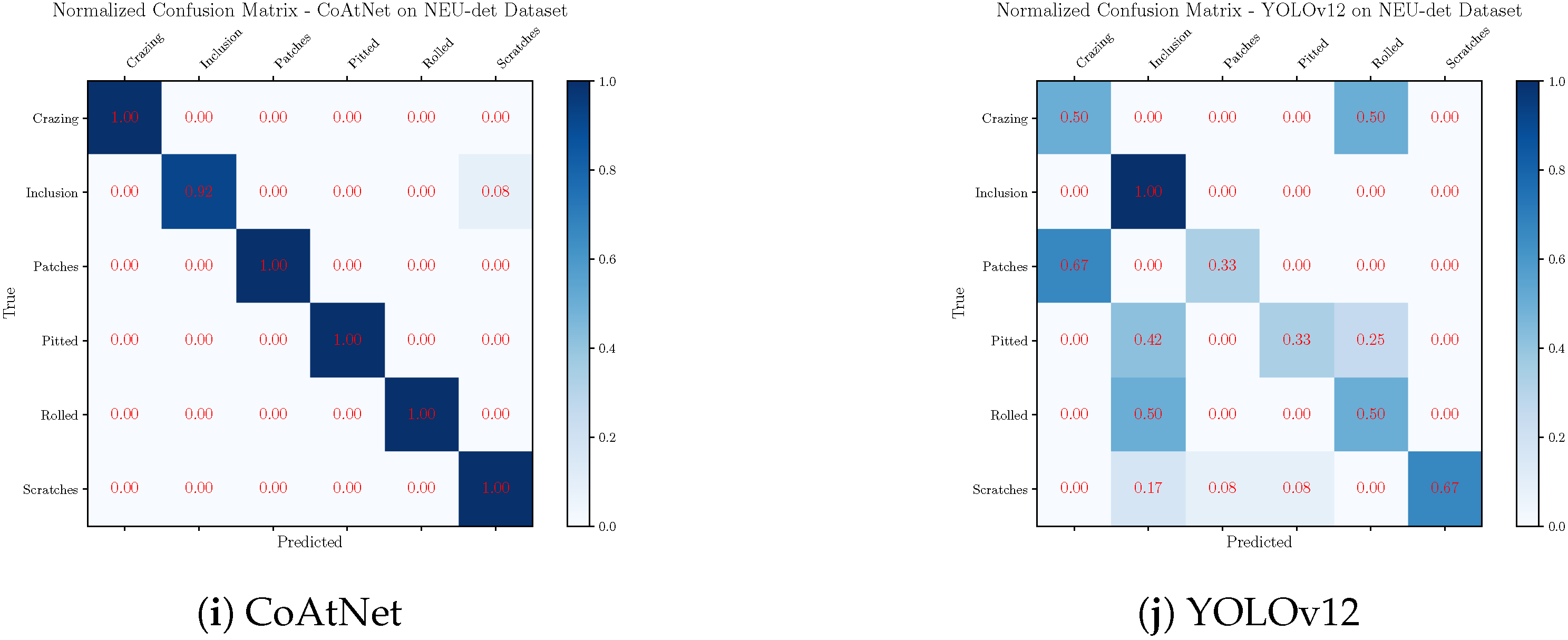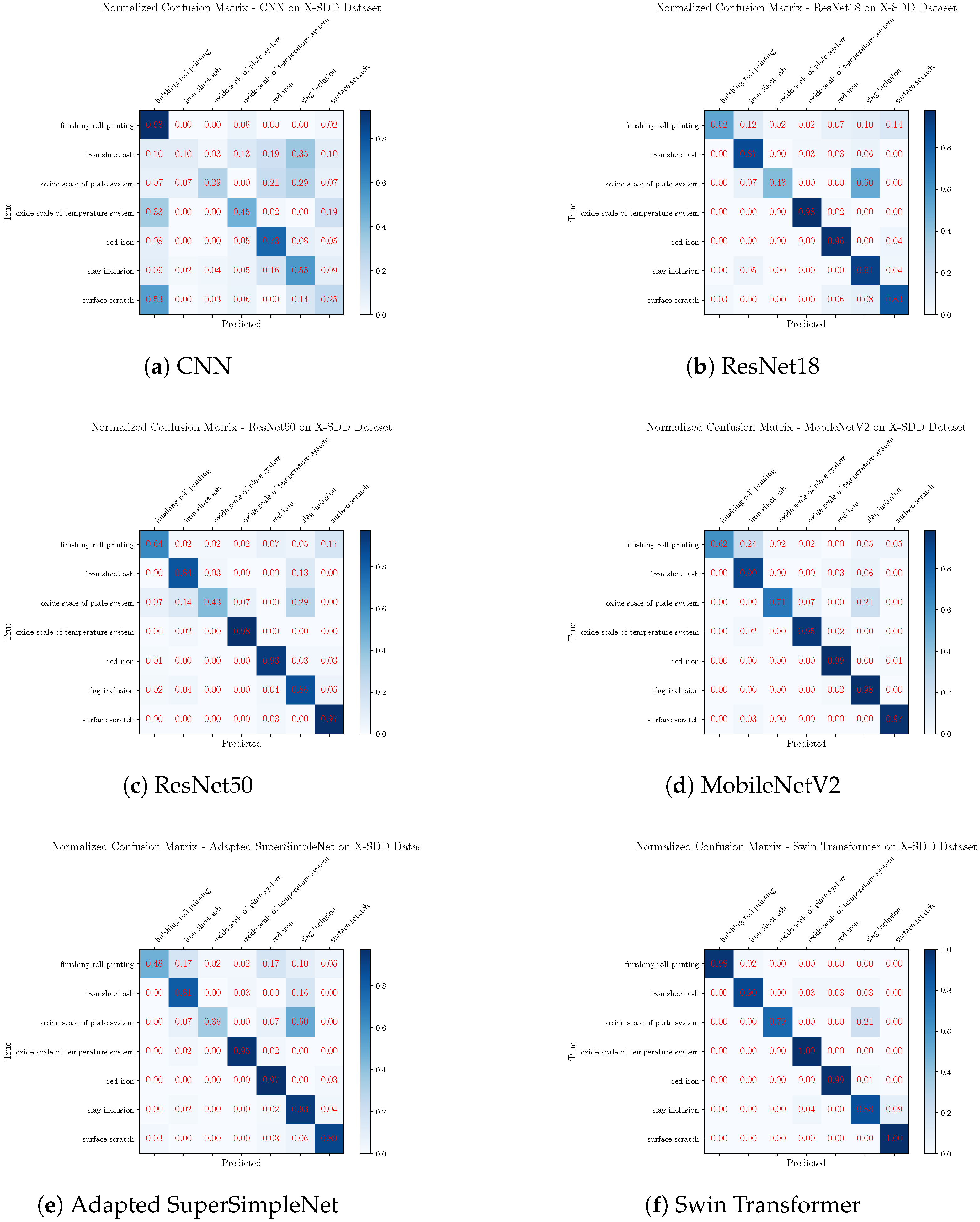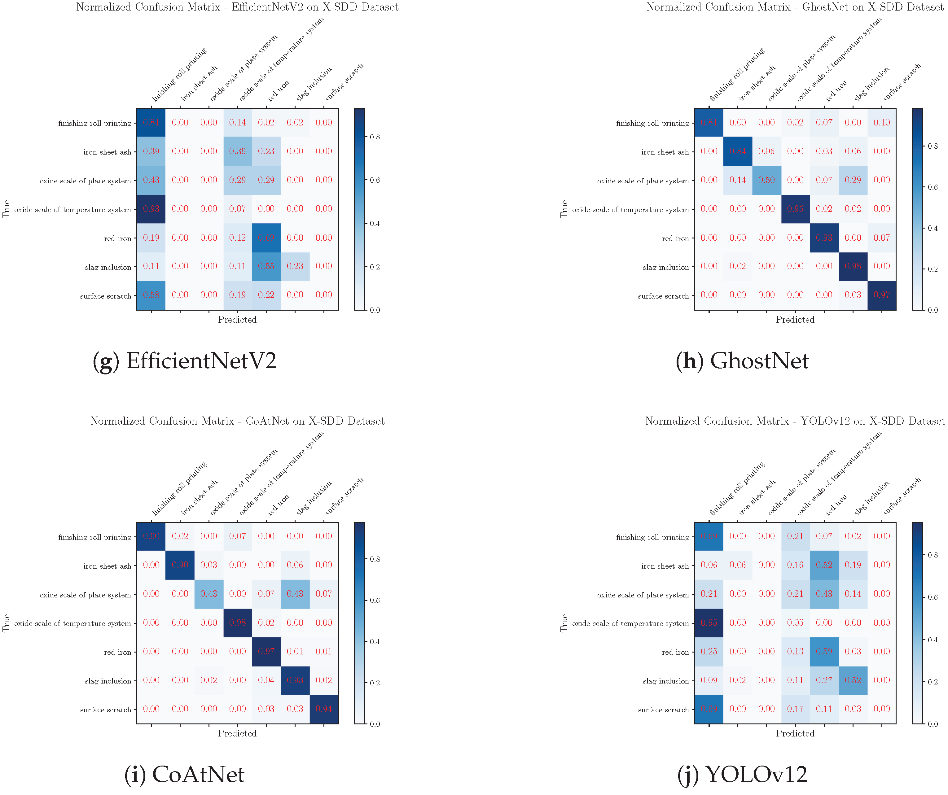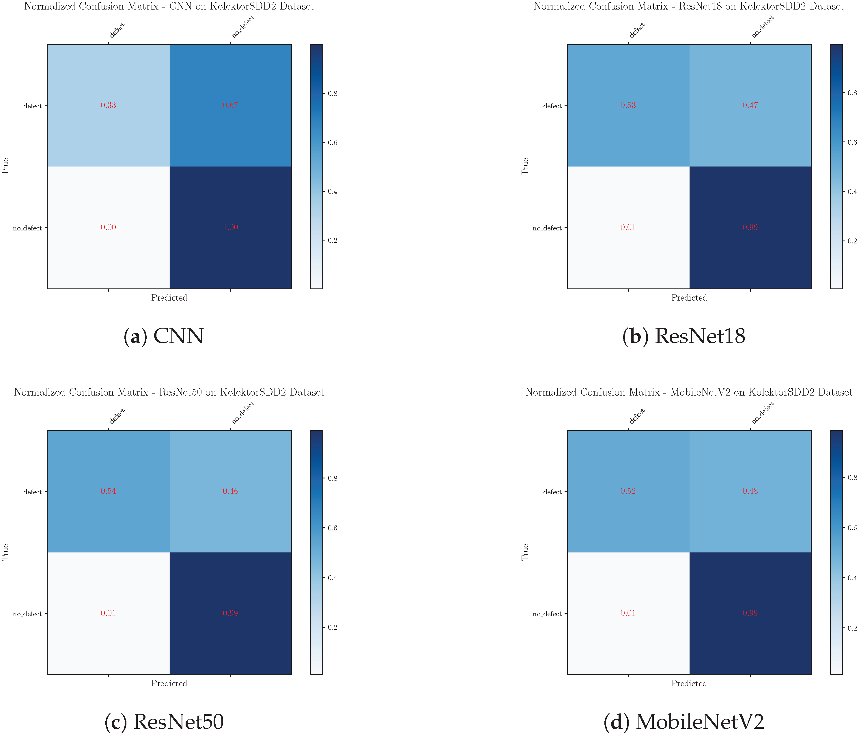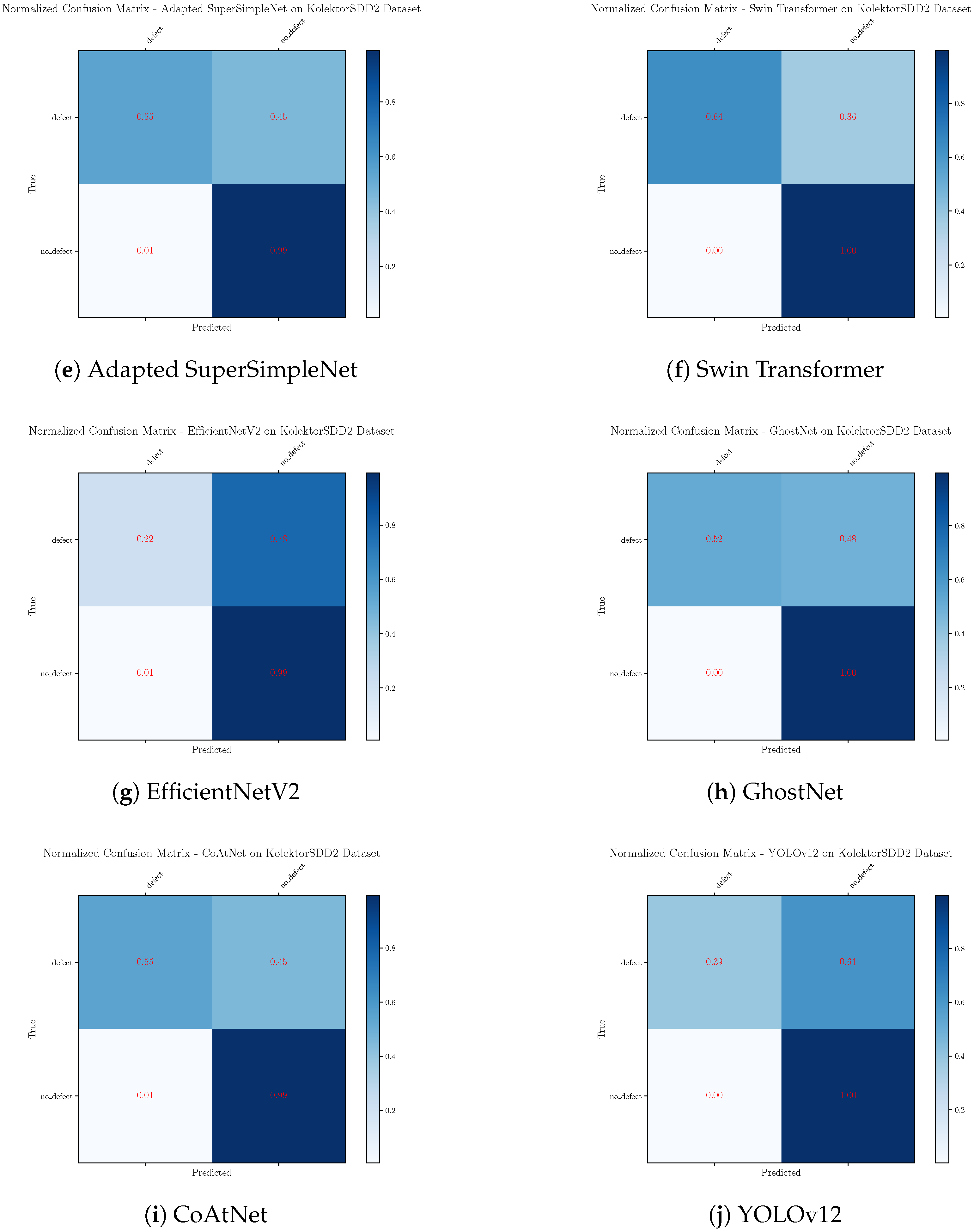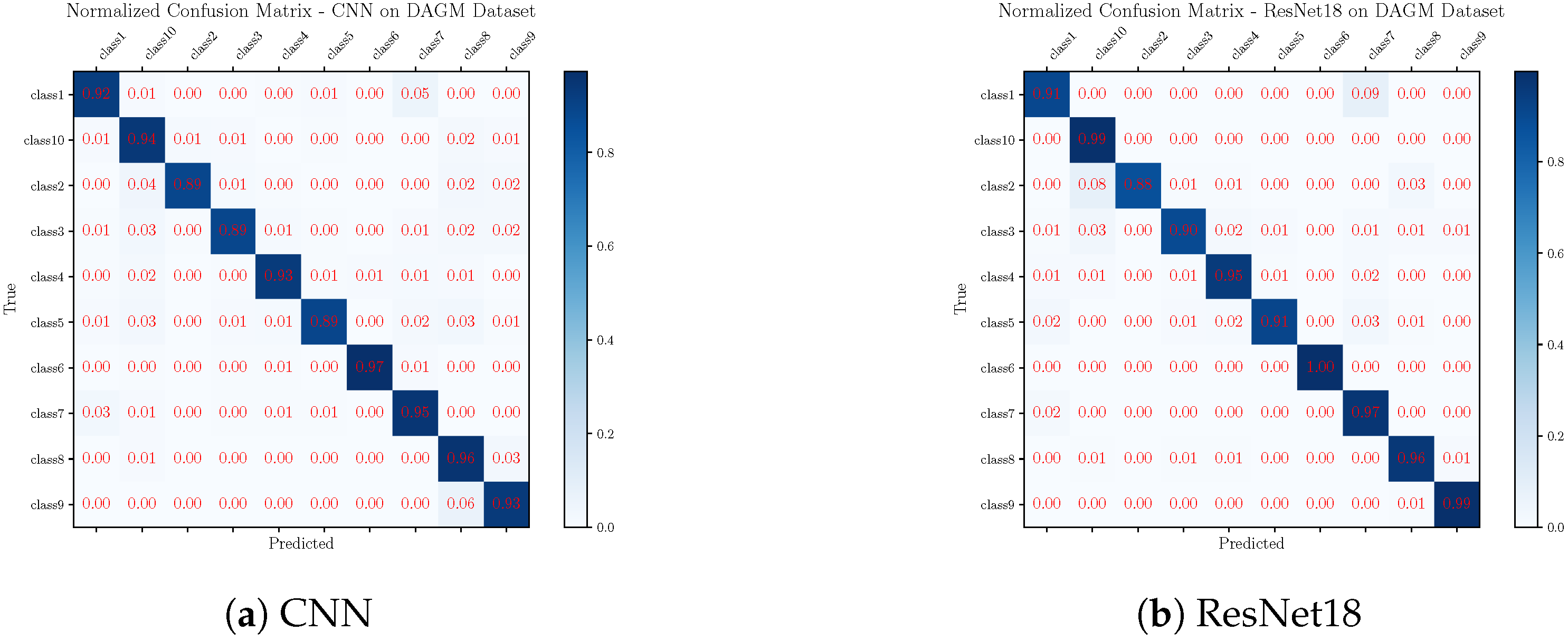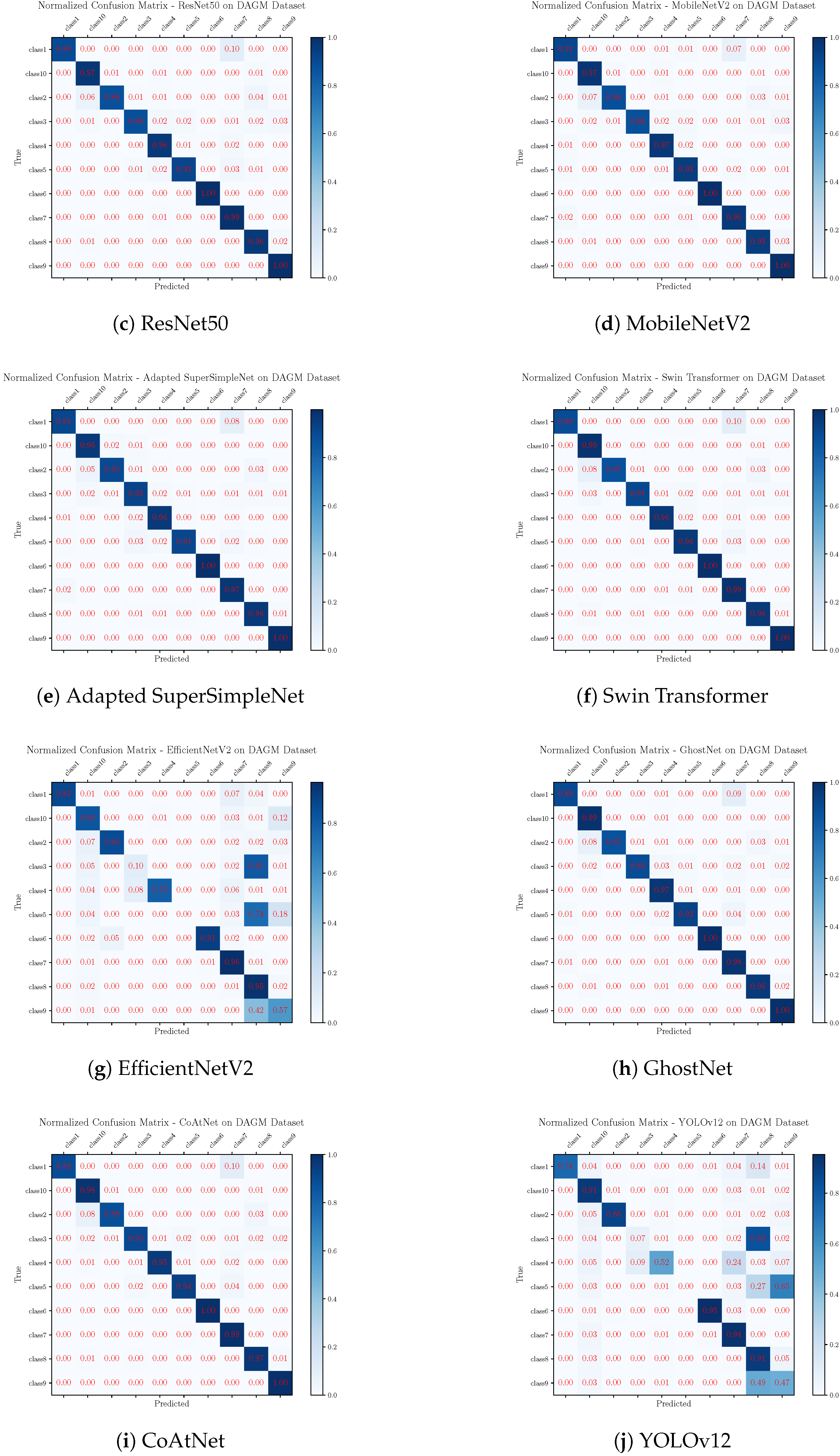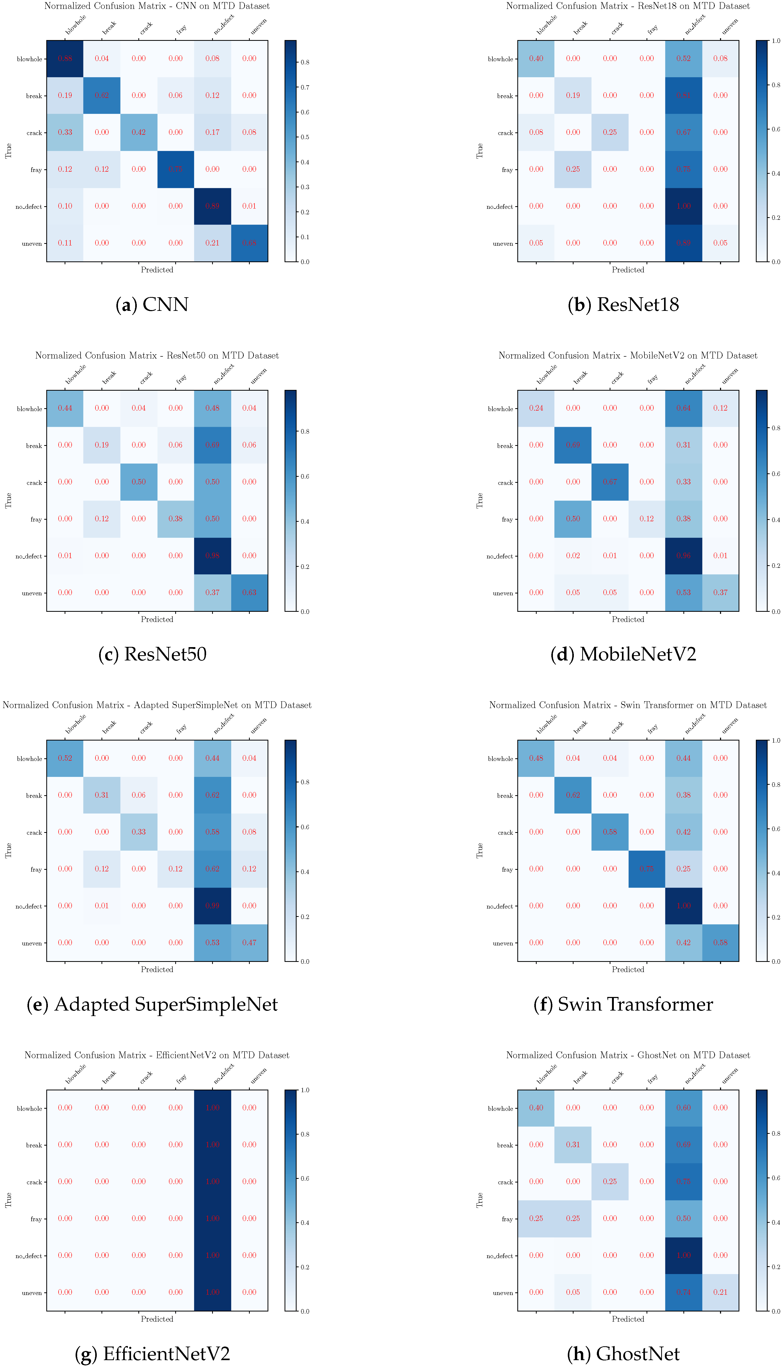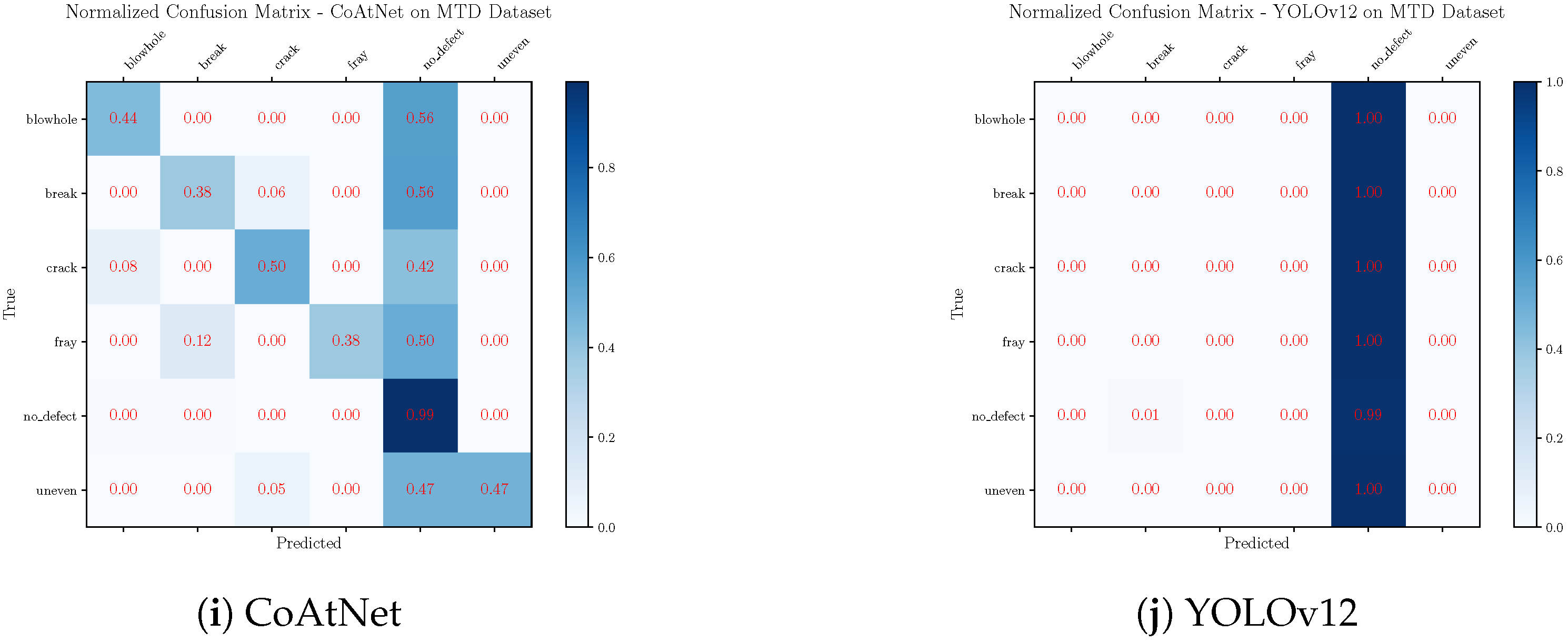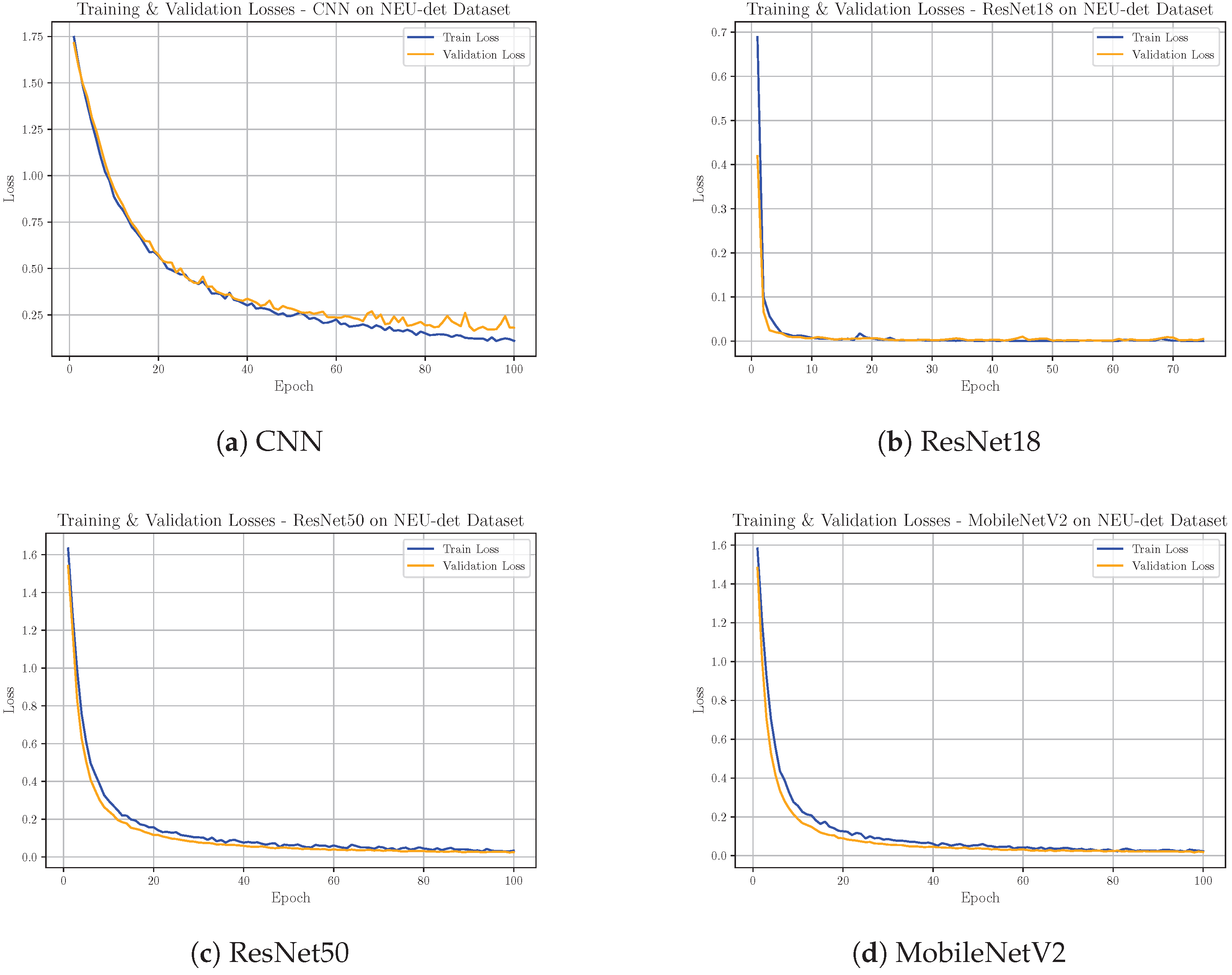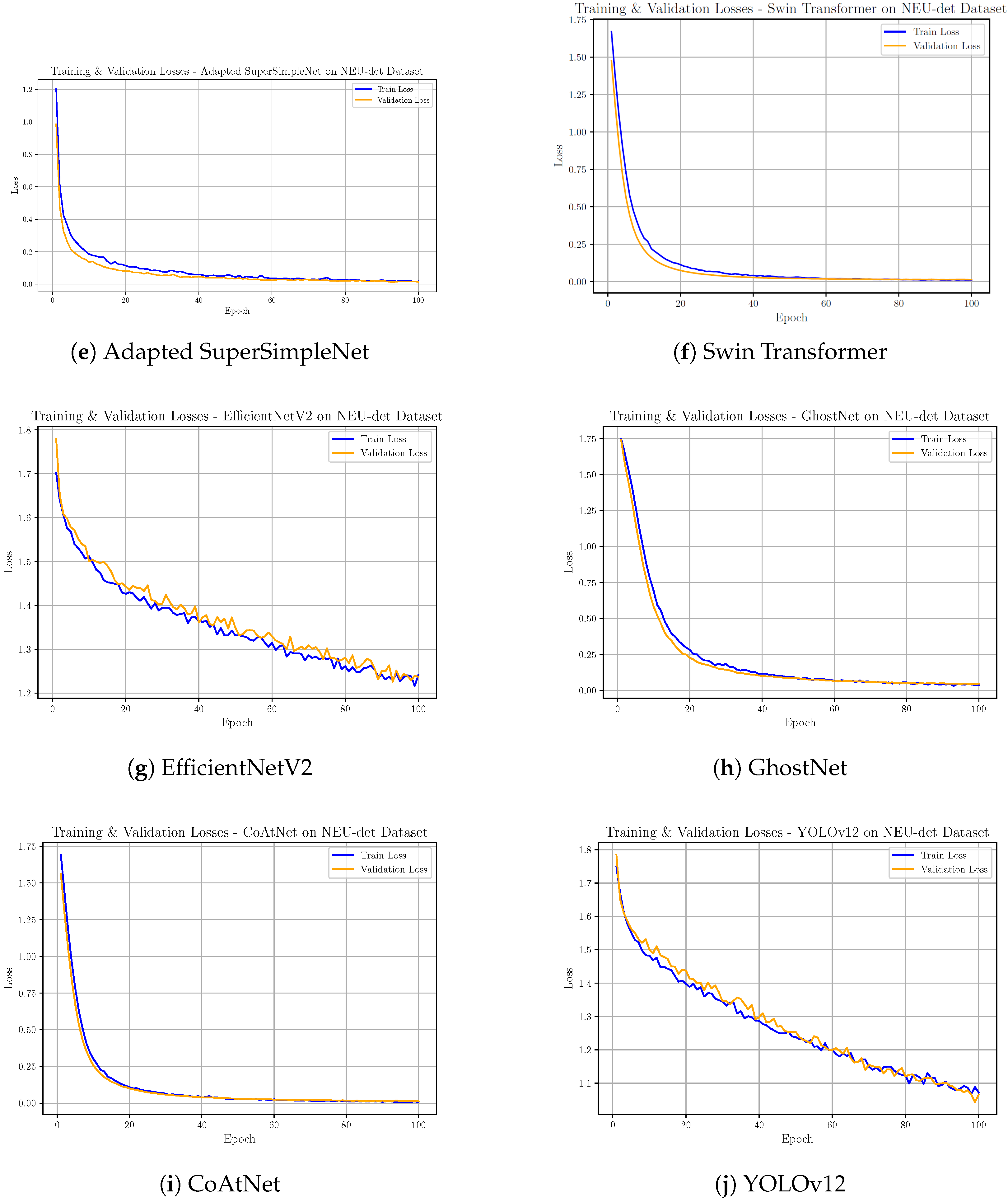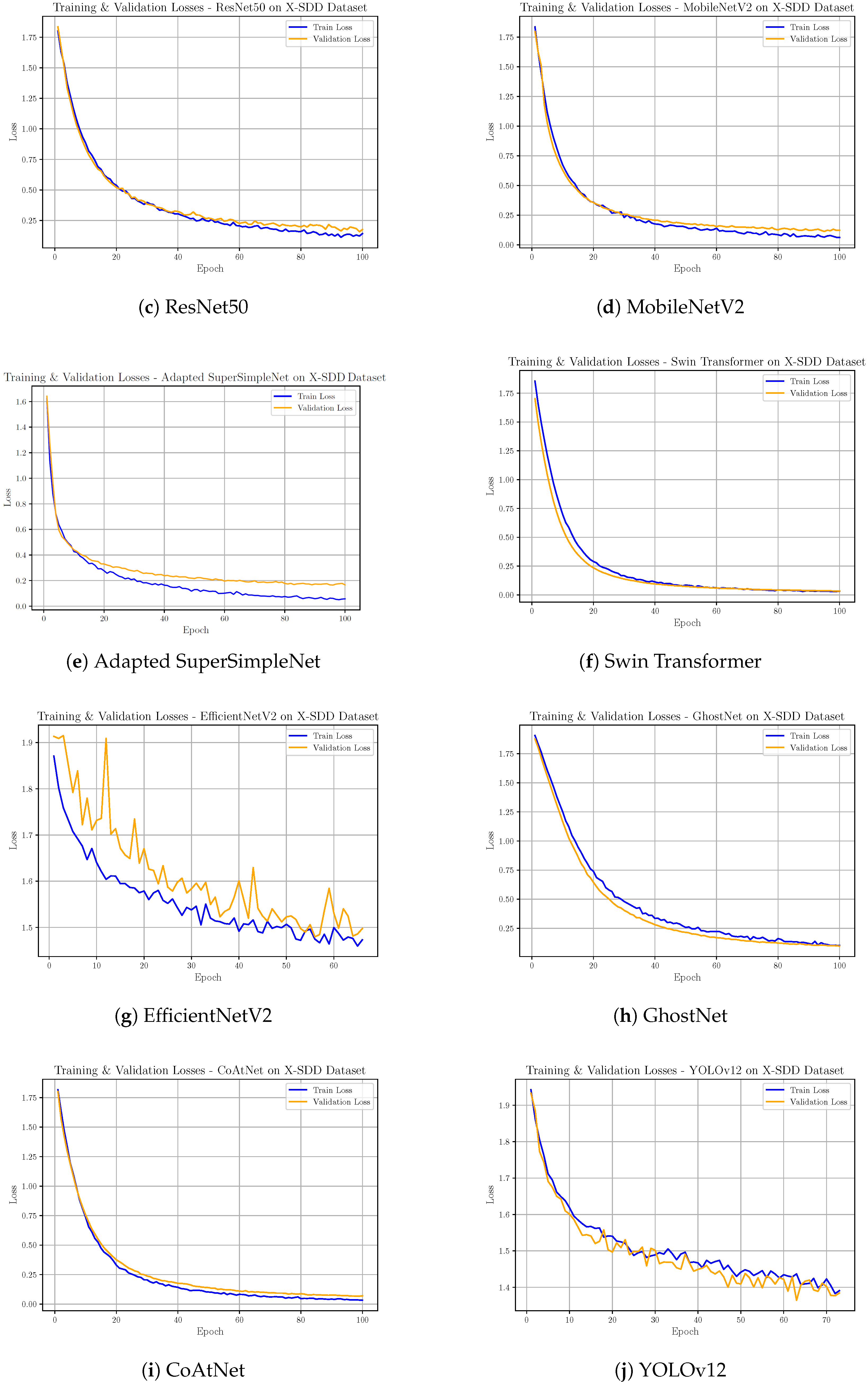Section 6 concludes the article by providing key insights, highlighting the novelty of this benchmark, and outlining topics for future research. 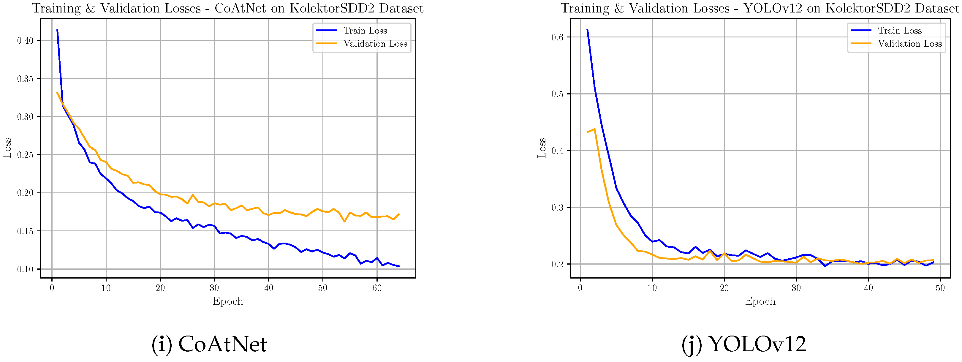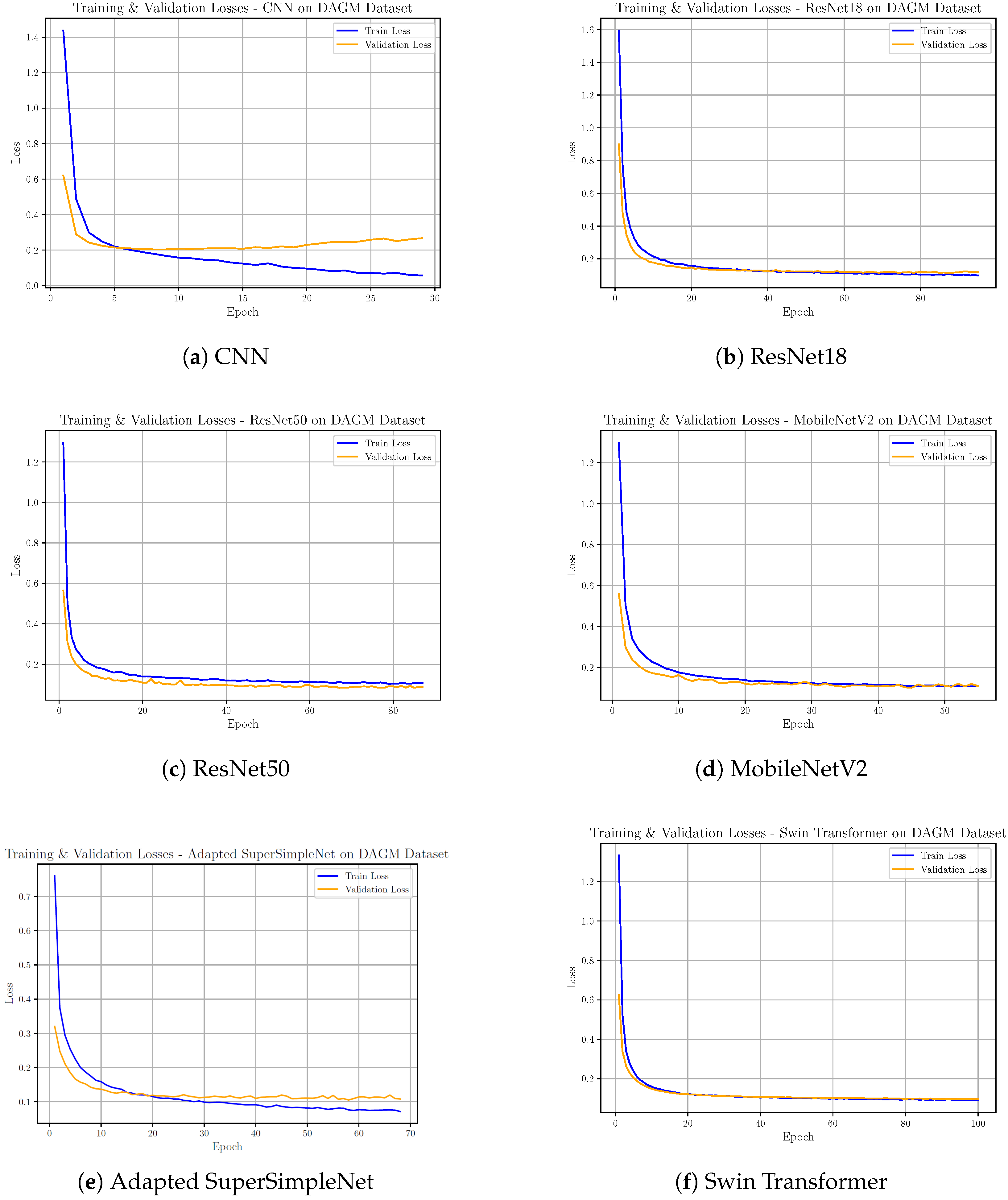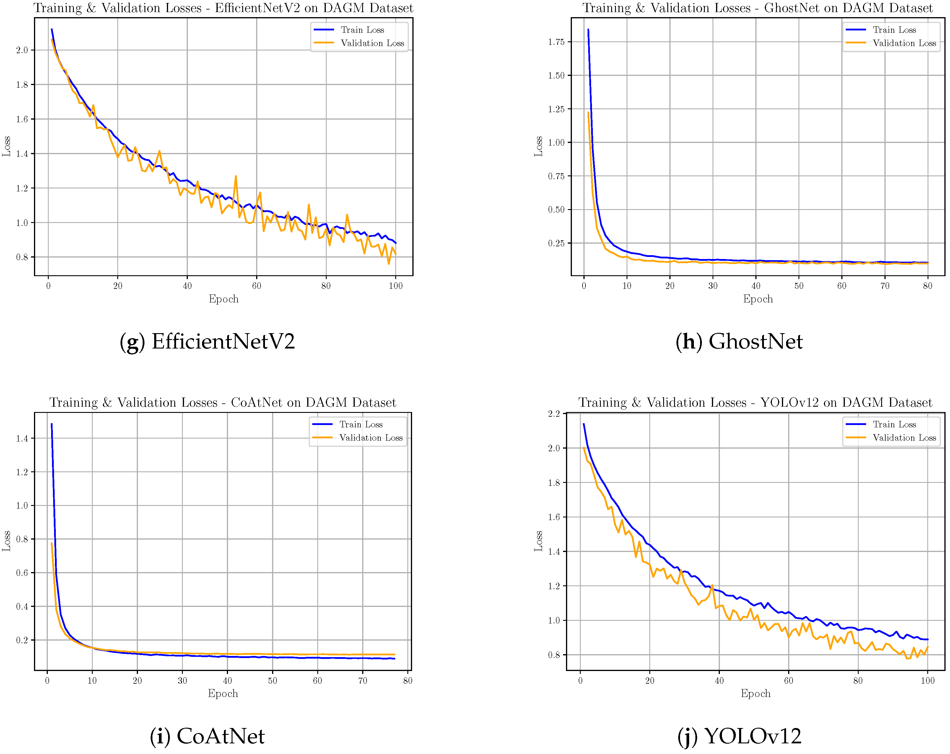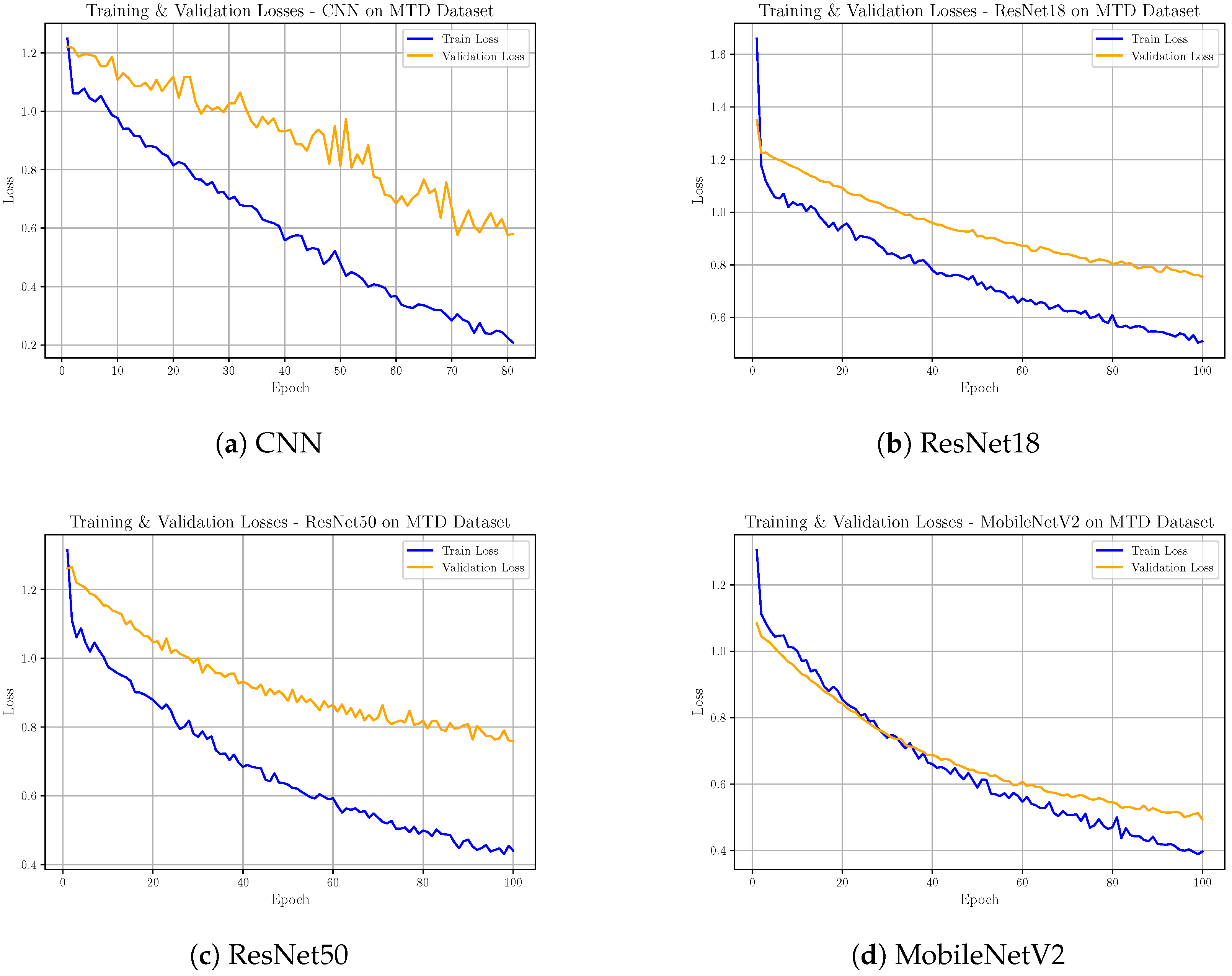Finally, the appendices complement the main text with confusion matrices (Appendix A) and loss plots for all models and datasets (Appendix B), offering additional diagnostic insights.

3. Methodology

This section presents the methodological framework adopted to systematically evaluate ten state-of-the-art deep learning architectures for surface defect classification. The methodology integrates three core elements: the datasets used for benchmarking, the models under comparison, and the training and evaluation protocol.

Performance comparison was based on standard classification metrics—accuracy, precision, recall, and F1-score—measured on held-out test sets. The training and the per-image inference latency for each model were also recorded to capture deployment feasibility. All experiments were conducted under identical conditions using the same hardware configuration: an NVIDIA GeForce RTX 4070 Laptop GPU, Intel(R) Core(TM) i7-14650HX @ 2.20 GHz CPU, and 32.0 GB RAM. This uniform setup ensures fair and reproducible comparisons across architectures.

3.1. Datasets

The training and evaluation were applied to five benchmark datasets: the Northeastern University Surface Defect Database (NEU-DET), X-SDD, KolektorSDD2, DAGM, and the Magnetic Tile Defects Dataset (MTDD). Among these, the first four are widely recognized as standard benchmarks in surface defect classification research. At the same time, MTDD introduces an additional domain with distinct defect types, further testing the generalization capability of the evaluated models.

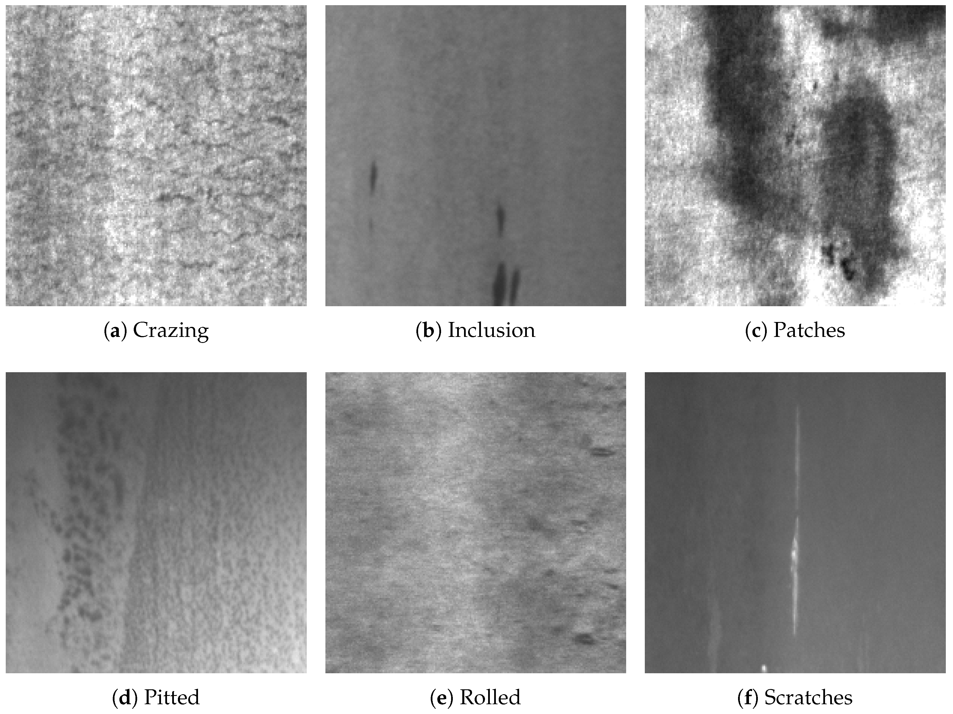
The Northeastern University Surface Defect Database (NEU-DET) https://www.kaggle.com/datasets/kaustubhdikshit/neu-surface-defect-database (accessed on 9 July 2025) consists of 1800 grayscale images, each of size $200\times 200$ pixels and 8-bit pixel depth, six classes, with 300 images per class [13]. The dataset covers six common surface defects in hot-rolled steel: crazing, inclusion, patches, pitted surface, rolled-in scale, and scratches. Defects are typically represented as local regions with irregular patterns, varying in size and background contrast, as shown in the examples in Figure 1. Images are labeled at the image level for classification. The controlled acquisition ensures consistent illumination and background, making NEU-DET a balanced and widely used benchmark for defect classification. Overall, NEU-DET is considered a relatively low-complexity dataset due to its balanced classes, number of classes, controlled imaging, and clear defect appearance.

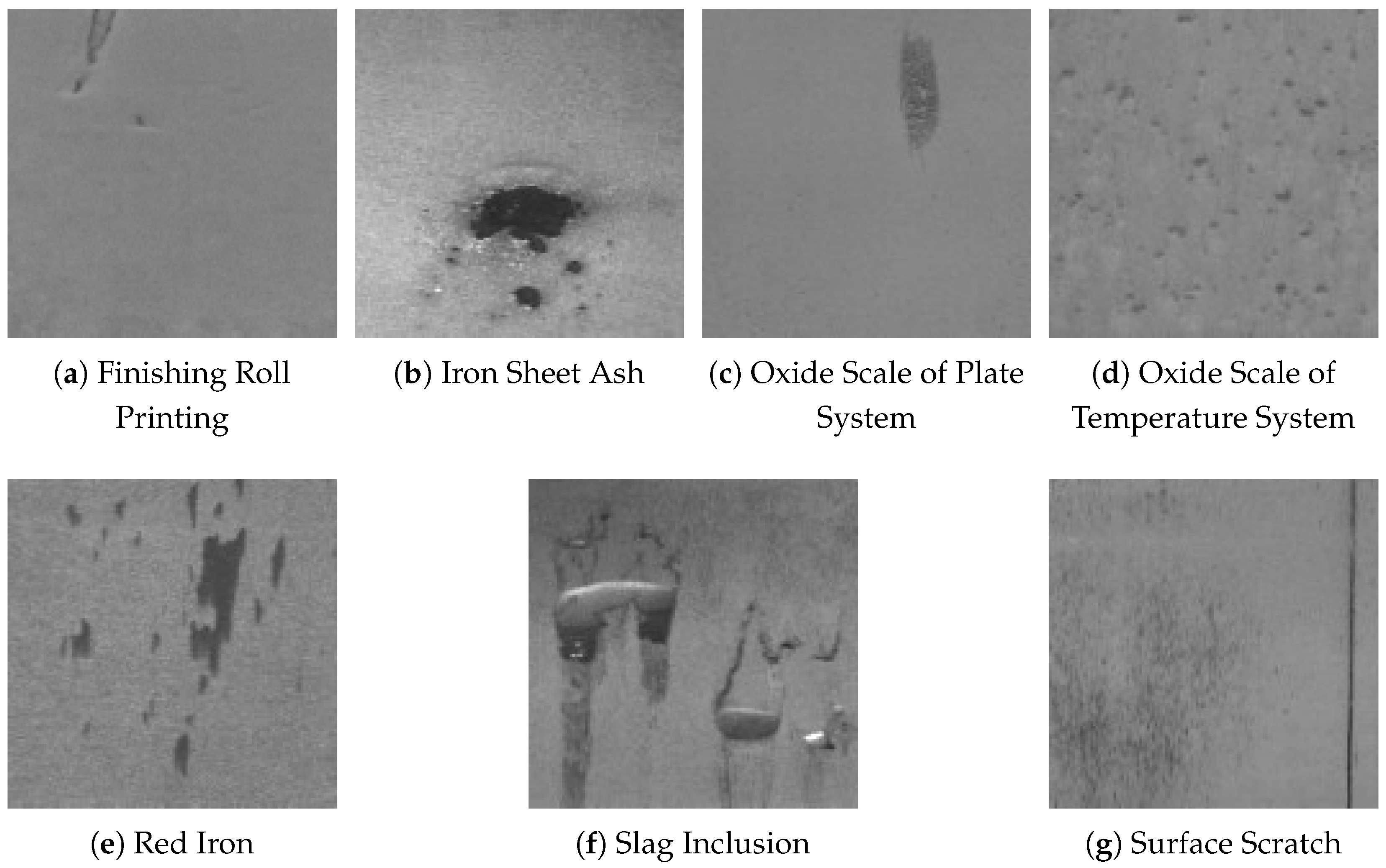
The X-SDD https://www.kaggle.com/datasets/sayelabualigah/x-sdd (accessed on 9 July 2025) dataset contains 1360 RGB images, each with a resolution of $400\times 400$ pixels and a pixel depth of 24 bits [14]. It includes seven defect categories: finishing roll printing, iron sheet ash, oxide scale of plate system, oxide scale of temperature system, red iron, slag inclusion, and surface scratch, with balanced representation per class. Defects are visually diverse, appearing as spots, lines, or textured regions, sometimes covering only a small part of the surface and varying in contrast and color, as shown in Figure 2. Images were collected under real steel manufacturing conditions, introducing realistic noise, illumination changes, and surface reflections. Annotations are provided at the image level for classification, with certain subsets also including localization or segmentation masks. Compared to NEU-DET, X-SDD introduces significantly higher complexity due to uncontrolled acquisition, varied illumination, and higher intra-class variability.

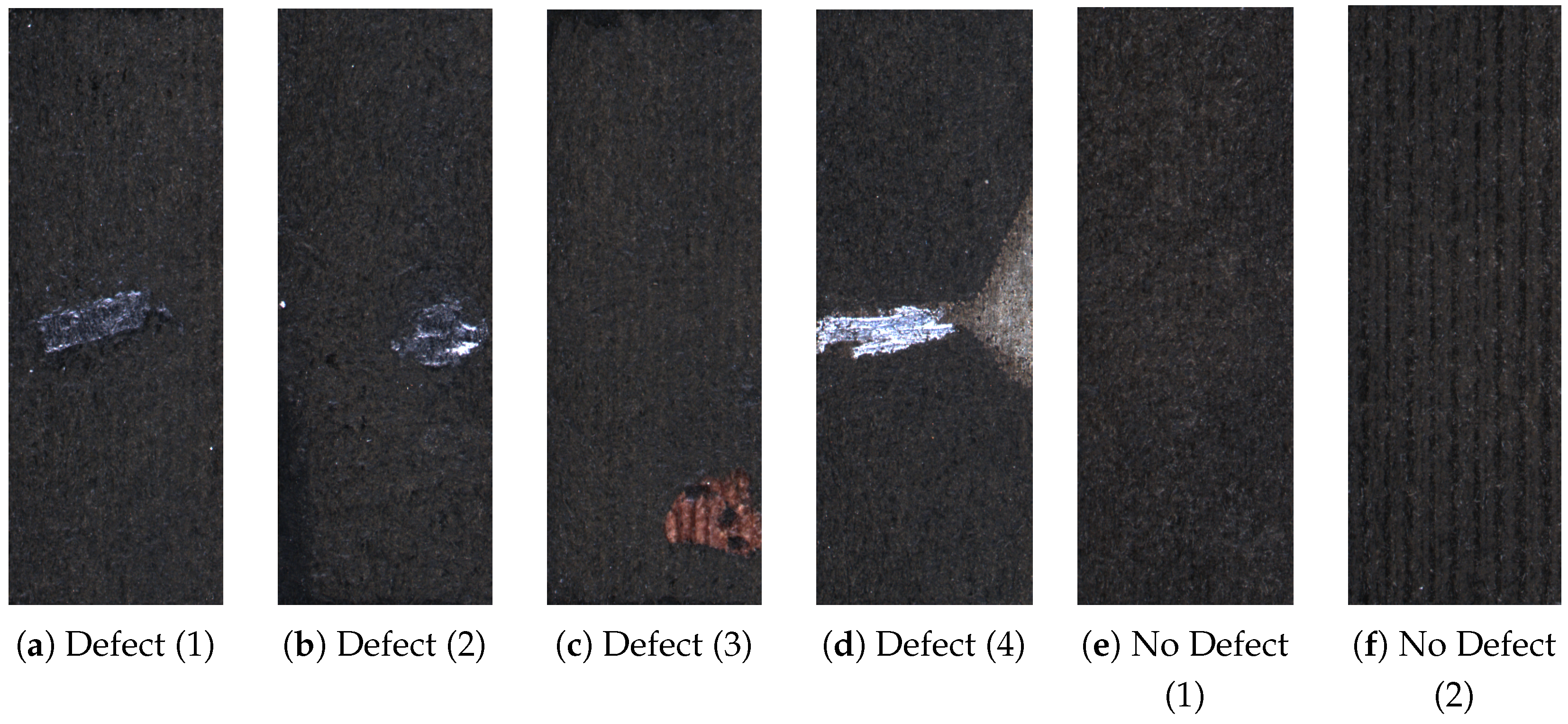
The Kolektor Surface-Defect Dataset 2 (KolektorSDD2) https://www.vicos.si/resources/ (accessed on 9 July 2025) dataset comprises 3326 high-resolution RGB images ($2300\times 1260$ pixels, 24-bit color depth) acquired from industrial production lines [15]. Defect types include scratches and various fine, irregular anomalies; 300 images with at least one defect, and the remaining represent non-defective surfaces. Defects are often subtle, small, or visually similar to the background, posing a significant challenge for detection, as shown in Figure 3. Both image-level and pixel-level (bounding box and segmentation mask) annotations are available. The dataset reflects practical industrial variability in illumination, background, and defect shape. This makes KolektorSDD2 a high-complexity dataset, where small, low-contrast defects are easily confused with background texture, pushing models beyond simple feature discrimination.

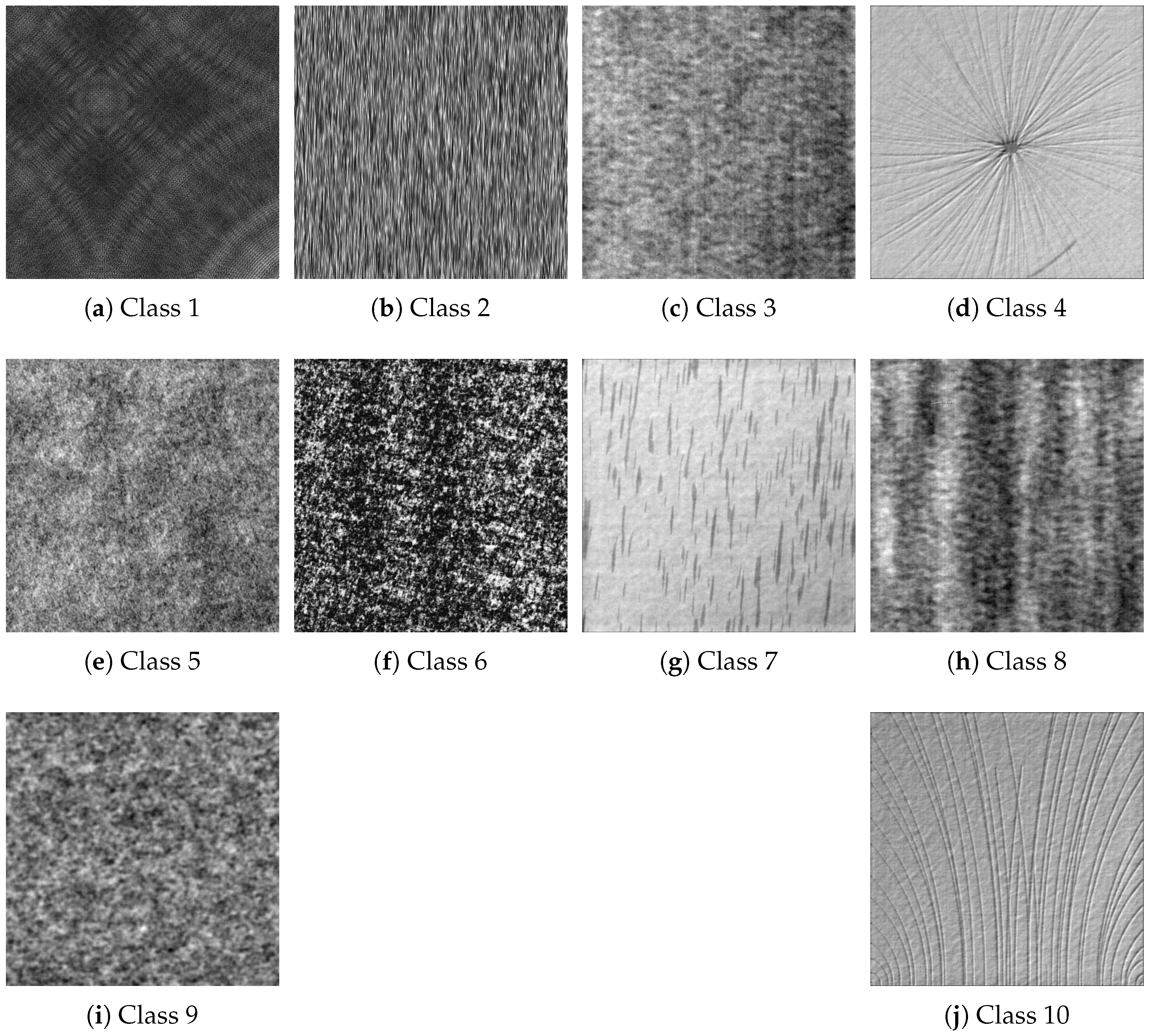
The DAGM 2007 competition https://www.kaggle.com/datasets/mhskjelvareid/dagm-2007-competition-dataset-optical-inspection (accessed on 9 July 2025) dataset consists of 10,000 grayscale images, each $512\times 512$ pixels at 8-bit depth [16,17]. The images are divided into ten classes, each simulating a different synthetic texture with artificially introduced defects such as spots, scratches, blobs, and texture anomalies. Defects are generally localized, varying in size, shape, and position, and often present low contrast against the patterned background, as shown in Figure 4. Each image is annotated at the pixel level, with segmentation masks identifying defective regions. The synthetic nature and controlled conditions allow a precise benchmarking, though they may not fully represent the variability of real-world defects. In terms of complexity, DAGM occupies a middle ground: while synthetic textures make it more controlled than industrial datasets like X-SDD or KolektorSDD2, the low-contrast defects within textured backgrounds still pose a significant challenge.

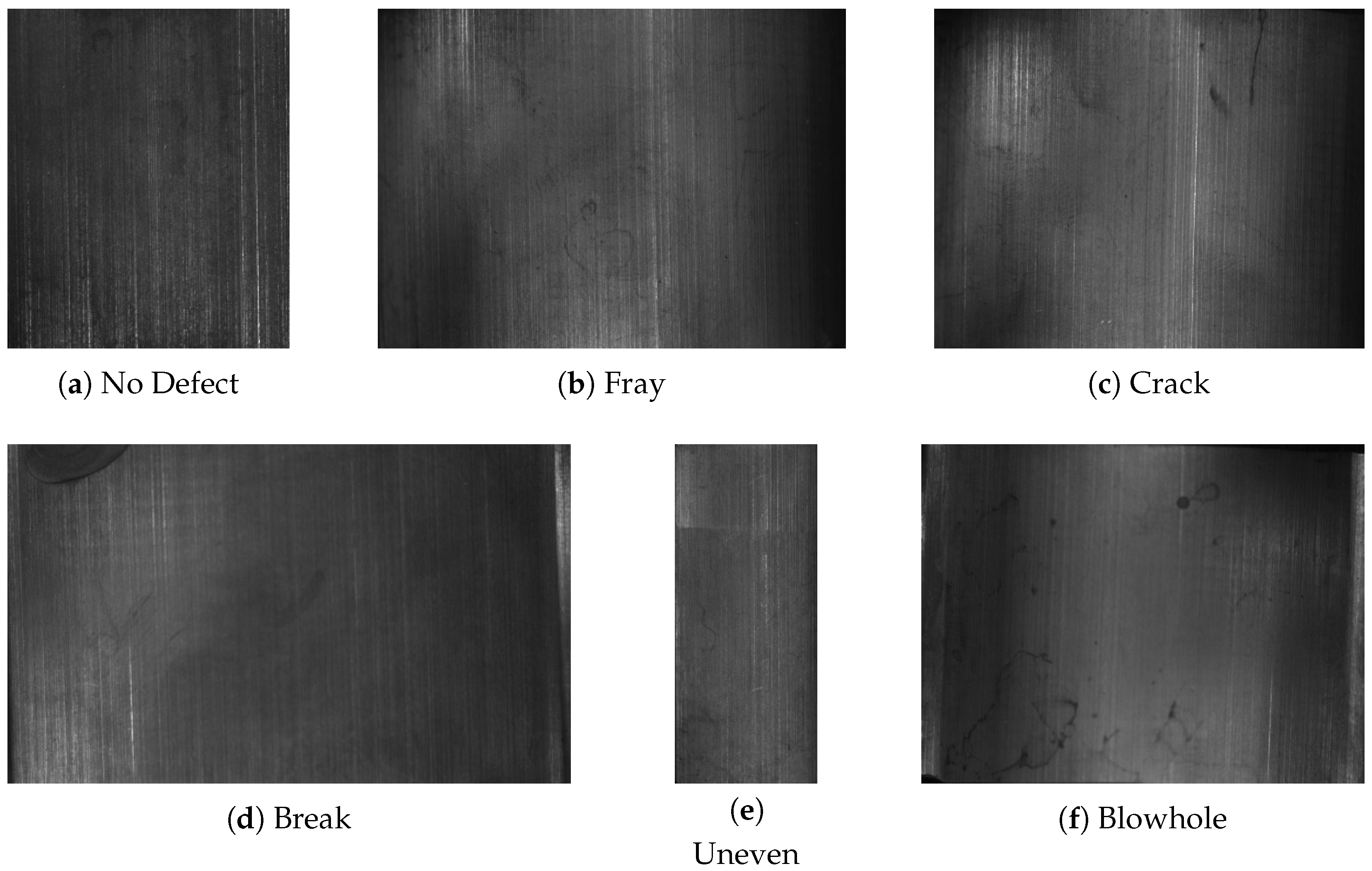
The Magnetic Tile Defects https://www.kaggle.com/datasets/alex000kim/magnetic-tile-surface-defects (accessed on 9 July 2025) dataset, shorted to MTDD, contains 1320 RGB images, with varying resolutions (typically ranging from $256\times 256$ to $400\times 400$ pixels) and 24-bit color depth [18]. It includes six defect types—blowhole, crack, fray, break, uneven, and non-defective surfaces—with approximately 180–240 images per category. Defects are visually distinct: blowholes and cracks appear as local holes or lines, frays and breaks are irregular edge anomalies, while unevenness affects larger surface areas, as shown in Figure 5. Images were acquired under varying illumination and backgrounds, introducing real-world noise, shadows, and reflection artifacts. Annotation is at the image level, but some subsets include bounding boxes or segmentation masks. MTDD is considered moderately complex, as defects are visually distinct, but acquisition variability (illumination, noise) introduces additional difficulty compared to controlled datasets.

Table 1. Comparison of the five benchmark datasets used in this study.

Dataset	#Images	Resolution	Bit Depth	#Classes	Complexity
NEU-DET	1800	200 × 200	8-bit (grayscale)	6	Low
X-SDD	1360	400 × 400	24-bit (RGB)	7	High
KolektorSDD2	3326	2300 × 1260	24-bit (RGB)	2	High
DAGM	10,000	512 × 512	8-bit (grayscale)	10	medium
MTDD	1320	variable	24-bit (RGB)	6	medium

summarizes the main characteristics of the datasets used, including the number of images, resolution, bit depth, classes, available annotations, and relative complexity to facilitate a clear comparison across datasets. This overview highlights the differences between controlled laboratory datasets (e.g., NEU-DET, DAGM) and industrial datasets collected under real-world conditions (e.g., X-SDD, KolektorSDD2, MTDD). Such differences are crucial for understanding each dataset’s varying levels of challenge for defect classification models and for interpreting the performance trends reported in the results.

Across the five benchmark datasets, the difficulty of defect evaluation is influenced by several interacting factors. These include the image resolution and colour space (grayscale or RGB), which affect the amount of spatial and chromatic information available, the number of classes and their balance, which influence the complexity of the classification task, and the acquisition conditions, such as controlled laboratory imaging versus real industrial environments with illumination changes, reflections, and noise. Additional factors include the size, contrast, and spatial extent of the defects, their similarity to the background texture, the degree of intra-class variability and inter-class overlap, and the type of annotation provided (image-level, bounding-box, or pixel-level). Together, these characteristics explain why some datasets, such as NEU-DET, are more suitable for controlled benchmarking, whereas others, such as X-SDD and KolektorSDD2, pose a substantially greater challenge for robust defect classification.

3.2. Models

The selected models range from simple, lightweight architectures to deeper and more complex networks, enabling a comprehensive analysis of the trade-offs between accuracy, efficiency, training and execution time, and deployment suitability.

Traditional CNN: A baseline architecture consisting of five convolutional layers followed by two fully connected layers was considered. Each convolutional block employs ReLU activation and max-pooling for feature extraction and dimensionality reduction. While relatively simple, this model is a strong benchmark for evaluating the benefits of deeper or more advanced architectures.

ResNet18 is an 18-layer residual neural network that introduces skip (shortcut) connections, allowing the model to mitigate vanishing gradient issues and train effectively at greater depth [19]. It balances performance and computational efficiency well, making it suitable for moderate-sized datasets or real-time applications where model depth is a consideration, as it contains only about 11.7M parameters and requires roughly 1.8 GFLOPs (FLOPs in AI refers to Floating-Point Operations, a metric for a model’s computational complexity, indicating the number of decimal-point calculations needed for a single run or task) per $224\times 224$ input, significantly less than deeper variants such as ResNet50 (∼25M parameters, ∼4.1 GFLOPs), while still achieving competitive accuracy in many vision tasks. Its relatively shallow architecture, with 18 layers and about 11.7 million parameters, reduces computational cost compared to deeper ResNet variants, enabling faster training and inference on standard hardware. The residual connections enhance gradient flow, allowing effective learning despite the reduced depth. This makes ResNet18 ideal for scenarios requiring robust image classification performance without excessive resource demands, such as embedded systems, mobile applications, or rapid prototyping in Computer Vision tasks. For example, it is often used in transfer learning for tasks like object detection or segmentation, where its efficiency and accuracy provide a practical trade-off.

ResNet50 is a deeper, 50-layer residual neural network that expands on the principles of ResNet18 by incorporating bottleneck residual blocks, which reduce the number of parameters and computations per block while still enabling very deep feature extraction [19]. With approximately 25.6M parameters and about 4.1 GFLOPs per $224\times 224$ input, ResNet50 offers substantially higher representational capacity than ResNet18. Its depth allows it to capture subtle textures and complex patterns, making it especially effective for fine-grained classification tasks such as distinguishing between visually similar defect types. However, this comes at the cost of increased training time and higher hardware requirements, making it better suited to scenarios where accuracy is prioritized over computational efficiency.

MobileNetV2 is a compact and efficient model explicitly designed for mobile and edge applications [20]. It relies on depthwise separable convolutions, which decompose standard convolutions into depthwise and pointwise operations, dramatically reducing computation and parameter count. Additionally, it introduces inverted residuals with linear bottlenecks, which preserve representational power while keeping the model lightweight. With roughly 3.5M parameters and only 0.3 GFLOPs per $224\times 224$ input, MobileNetV2 is one of the fastest architectures tested, making it highly attractive for real-time deployment on resource-constrained platforms without sacrificing too much accuracy.

Adapted SuperSimpleNet is a lightweight convolutional neural network tailored for surface defect detection. Building on the original SuperSimpleNet [21], this adapted version increases classification capacity while maintaining its hallmark low parameter count and extremely fast training time. With fewer than 1M parameters and negligible FLOPs, it emphasizes speed, simplicity, and ease of deployment. Its efficiency makes it highly practical for rapid prototyping or embedded scenarios, although its limited depth constrains its ability to generalize on more complex datasets compared to deeper architectures.

Swin Transformer is a hierarchical vision transformer that introduces the shifted-window attention mechanism, restricting self-attention computation to local windows and then shifting them between layers [22]. This design reduces computational cost compared to global attention while still capturing long-range dependencies. The hierarchical representation, akin to CNN feature pyramids, enables scalability to high-resolution images, with strong performance on tasks requiring global context. Although it is more computationally demanding than lightweight CNNs, Swin Transformer excels at modeling subtle surface defect patterns and has proven to generalize well across diverse datasets.

EfficientNetV2 is an improved variant of EfficientNet designed for faster training and higher accuracy [23]. It incorporates fused MBConv layers, which replace depthwise separable convolutions in early layers, progressive learning strategies, and optimized scaling rules to balance depth, width, and resolution. This results in faster convergence and reduced training time compared to earlier EfficientNet versions. With parameter counts ranging from a few million to tens of millions depending on the variant, EfficientNetV2 is well-suited for contexts where training efficiency and high accuracy are both critical.

GhostNet is a highly efficient architecture that introduces “ghost modules” to generate additional feature maps from cheap linear operations, significantly reducing the redundancy of standard convolutions [24]. This design allows GhostNet to achieve competitive accuracy while using a fraction of the parameters and FLOPs of comparable CNNs. With around 5M parameters and extremely low computational demand, it is particularly attractive for real-time applications and embedded systems where inference speed and memory efficiency are paramount.

CoAtNet is a hybrid architecture that combines the strengths of convolutional layers and self-attention mechanisms [25]. Convolutions provide strong inductive biases and efficient local feature extraction, while attention layers capture global dependencies and long-range interactions. This hybrid design enables CoAtNet to scale effectively across both small and large datasets, balancing the efficiency of CNNs with the representational power of transformers. It is especially well-suited to applications requiring robustness across diverse textures and defect scales, albeit with higher computational demands compared to lightweight CNNs.

YOLOv12 is the latest one-stage detector from the YOLO family, optimized for real-time performance [26]. In its original form, YOLOv12 performs object detection through a backbone, neck, and detection head pipeline. For this study, YOLOv12 was adapted into a classifier by removing its detection heads and retaining the backbone for feature extraction, followed by global pooling and a fully connected classification head. This adaptation preserves YOLOv12’s efficient backbone design while aligning it with the classification task, allowing direct comparison with other models in this benchmark. Although not originally designed for classification, its streamlined backbone provides competitive performance, especially in scenarios emphasizing speed.

Table 2. Comparison of models regarding parameter count, computational complexity, and estimated inference speed.

Model	Parameters (Approx.)	FLOPs (224×224)	Estimated Speed
Traditional CNN	∼1M	Low	Fast
ResNet18	∼11.7M	∼1.8 GFLOPs	Moderate
ResNet50	∼25.6M	∼4.1 GFLOPs	Slower
MobileNetV2	∼3.5M	∼0.3 GFLOPs	Very Fast
Adapted SuperSimpleNet	∼0.5–1M	Very Low	Very Fast
Swin Transformer	∼88M	∼15 GFLOPs	Moderate-Slow
EfficientNetV2	∼24M	∼3.5 GFLOPs	Moderate
GhostNet	∼5.2M	∼0.14 GFLOPs	Very Fast
CoAtNet	∼27M	∼4.2 GFLOPs	Moderate
YOLOv12 (classifier)	∼7–10M	∼1–2 GFLOPs	Fast

provides a comparative overview of the ten selected models. For each architecture, the table reports the approximate number of parameters, the computational complexity measured in FLOPs for an input size of $224\times 224$ pixels, and a qualitative estimate of inference speed. This comparison highlights the spectrum of model capacities, from ultra-lightweight designs (e.g., SuperSimpleNet, GhostNet) to hybrid or transformer-based models (e.g., CoAtNet, Swin Transformer), offering a reference for assessing the trade-offs discussed in subsequent sections.

3.3. Training, Validation and Test Setup

A standard train-validation-test protocol was used to evaluate each model. For each dataset, the images were previously organized into training, validation, and test folders using a 65%/15%/20% split, respectively. Pre-processing consisted of resizing all input images to $224\times 224$ and converting them to tensors, scaling pixel intensities to the [0, 1] range using ToTensor(). No additional data augmentation, such as rotations, flips, or illumination perturbations, was applied. Likewise, no mean or standard normalization was used. Training was performed with a batch size of 32. The following steps were applied to each model:

1.

The model architecture was dynamically imported from its corresponding Python module, initialized with the required number of output classes, and moved to the available GPU.

2.

The Adam optimizer was used with a learning rate of $2.5\times {10}^{-5}$ and a weight decay of $1\times {10}^{-5}$. Cross-entropy loss served as the objective function.

3.

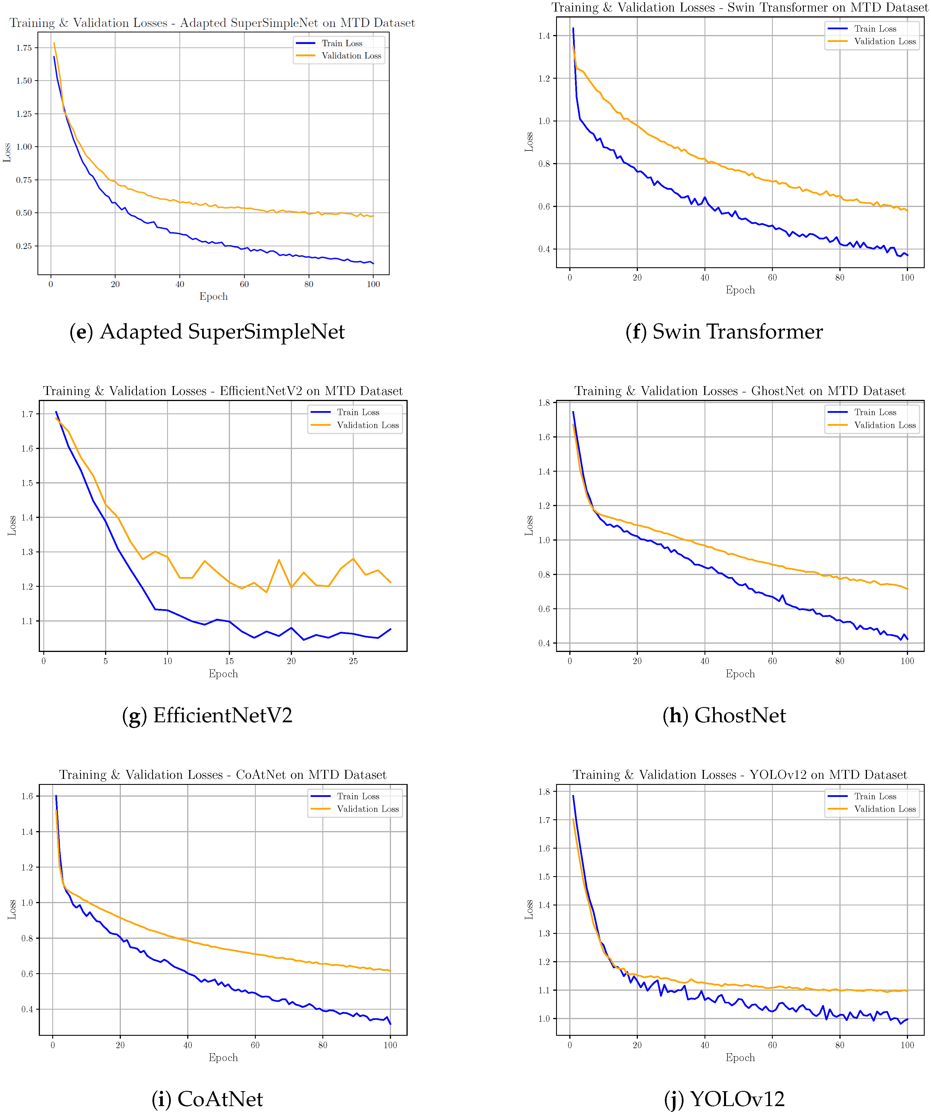
Each model was trained for up to 100 epochs. Early stopping was employed: if the validation loss did not improve for 10 consecutive epochs, training was halted.

4.

In each epoch, the model was trained on mini-batches from the training set, and the average training loss was recorded.

5.

After each epoch, the model was evaluated on the validation set without gradient updates, and the validation loss was computed.

6.

The model state corresponding to the lowest validation loss was saved for subsequent evaluation.

7.

Upon completion of training, the best-performing model weights were reloaded, and the model was evaluated on the test set.

8.

The following evaluation metrics were computed: accuracy, precision, recall, and F1-score (all using macro averaging), as well as a normalized confusion matrix.

A unified optimization protocol was intentionally adopted for all architectures, including the use of the Adam optimizer, a learning rate of $2.5\times {10}^{-5}$, a batch size of 32, and the same early-stopping criterion. This design was chosen to ensure methodological consistency and a fair cross-model benchmark under a common training budget, rather than to maximize the performance of each architecture through model-specific hyper-parameter tuning. No explicit class-imbalance mitigation strategy, such as weighted loss functions, oversampling, or weighted sampling, was employed. 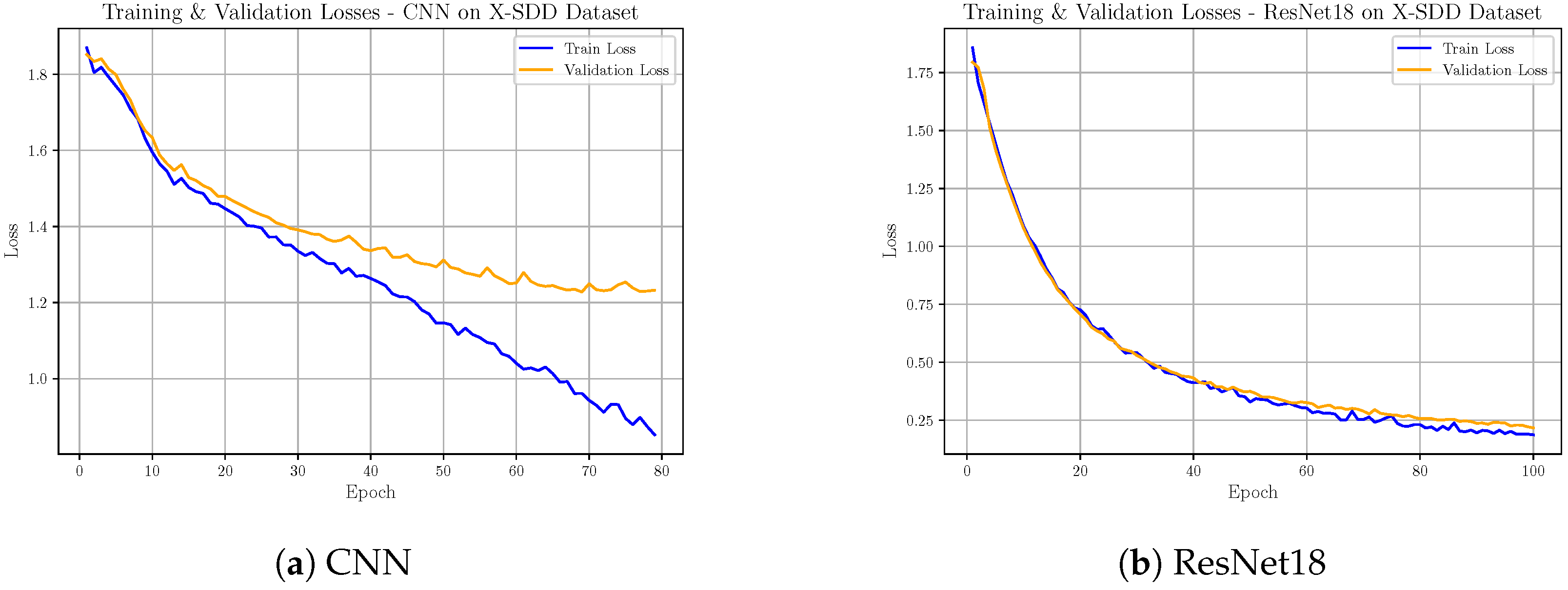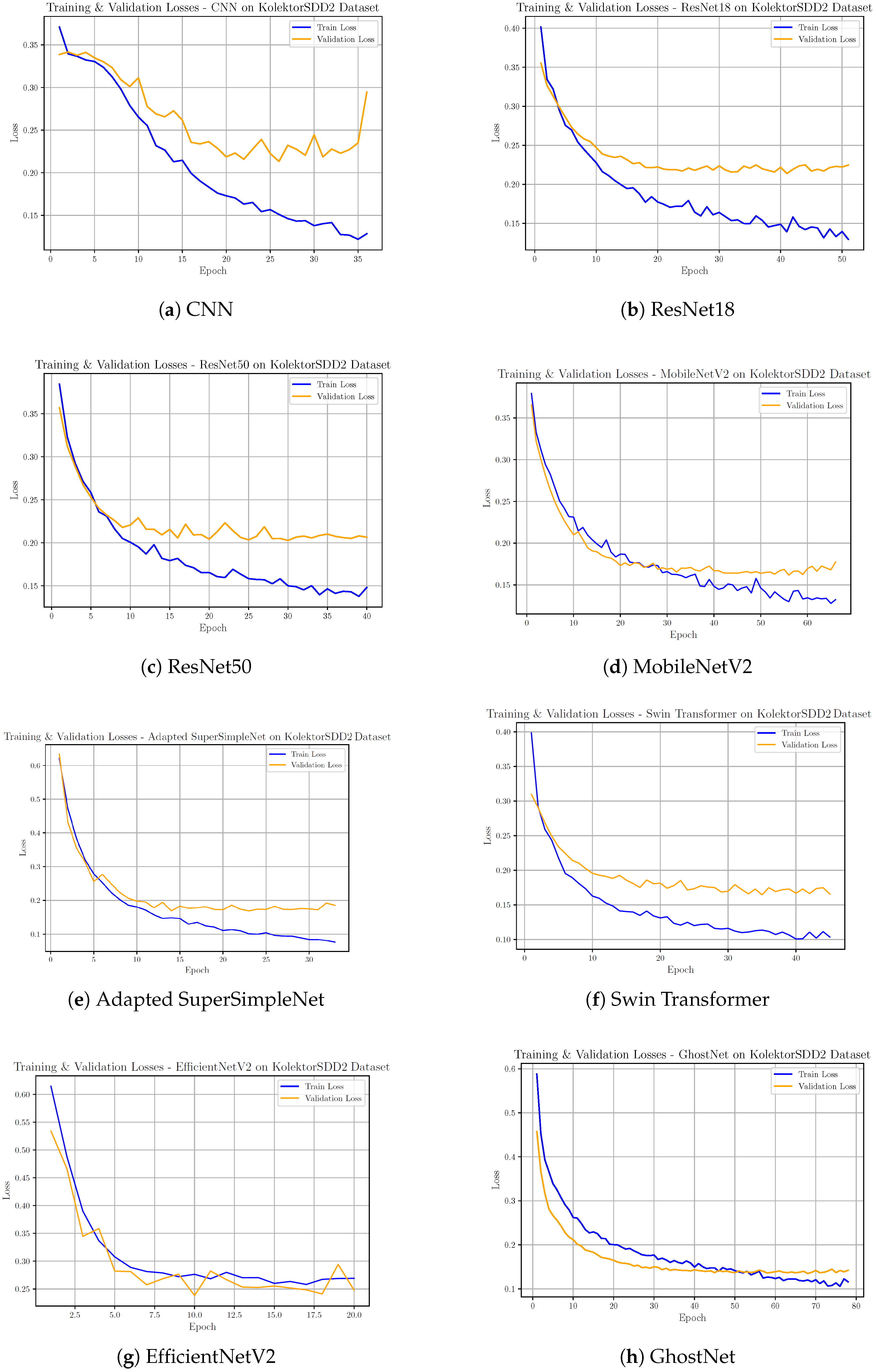In addition to the performance metrics computed from the confusion matrices generated during testing (Appendix A), ensuring a systematic basis for comparison, the pipeline outputs included: per-epoch training and validation losses (Appendix B), class label mappings, total training time, and the mean execution time for each model. To ensure reproducibility and efficient resource utilization, GPU memory was cleared and garbage collection was invoked after the evaluation of each model.

It should be noted that the objective of the present study is limited to defect identification and classification from image data. The proposed benchmark does not include downstream corrective actions, process adaptation, or closed-loop defect mitigation mechanisms.

4. Results

The comparison among the models under analysis was performed using standard classification metrics derived from the confusion matrix (

Table 3. Confusion Matrix Layout.

Predicted Class	True Class
	Positive	Negative
Positive	True Positive (TP)	False Positive (FP)
Negative	False Negative (FN)	True Negative (TN)

).

The metrics chosen for results extraction and further performance comparison between models were selected based on their ability to comprehensively evaluate classification effectiveness, especially in the context of defect classification, where class imbalance and misclassification costs may vary. These metrics allow for an in-depth assessment of both overall correctness and the model’s behaviour when distinguishing between defective and non-defective cases. The following standard classification metrics are used:

Accuracy represents overall prediction accuracy, defined as the proportion of correctly classified instances (both true positives and true negatives) over the total number of predictions:

$$Accuracy={\displaystyle \frac{TP+TN}{TP+FP+TN+FN}}={\displaystyle \frac{n_{correct}}{n_{total}}}$$

(1)

Precision assesses the quality of positive predictions, showing the ratio of true positive predictions to all positive predictions made by the model, where high precision indicates few false positives:

$$Precision={\displaystyle \frac{TP}{TP+FP}}$$

(2)

Recall, sometimes called the true positive rate, measures the model’s ability to identify actual positives, indicating the proportion of true positive predictions relative to all actual positive samples, where high recall means fewer false negatives:

$$Recall={\displaystyle \frac{TP}{TP+FN}}$$

(3)

F1-score, is especially useful in scenarios where false positives and false negatives carry different consequences, is the harmonic mean of precision and recall, balancing the trade-off between the two:

$$F1\text{-}\mathrm{score}={\displaystyle \frac{2·Precision·Recall}{Precision+Recall}}={\displaystyle \frac{2·\frac{TP}{TP+FP}·\frac{TP}{TP+FN}}{\frac{TP}{TP+FP}+\frac{TP}{TP+FN}}}={\displaystyle \frac{2·TP}{2·TP+FN+FP}}$$

(4)

The evaluation results across the five benchmark datasets are presented in the following. Each model was assessed using four standard classification metrics: accuracy, precision, recall, and F1-score. In addition, the training time required for each dataset is reported to provide insights into computational efficiency, and per-image inference latency is measured as an indicator of real-time deployment feasibility.

In

Table 4. Accuracy of each studied model across benchmark datasets. Cell colours are used to facilitate rapid visual comparison of relative performance, with green indicating higher accuracy, yellow indicating mid-range accuracy and red indicating lower accuracy.

Model	NEU-DET	X-SDD	KolektorSDD2	DAGM	MTDD
CNN	94.4%	54.1%	92.5%	93.1%	83.7%
ResNet18	100%	84.1%	94.3%	95.6%	79.0%
ResNet50	100%	85.5%	94.1%	95.6%	83.7%
MobileNetV2	100%	90.5%	93.5%	95.3%	81.7%
Adapted SuperSimpleNet	100%	83.5%	93.8%	95.5%	83.0%
Swin Transformer	100%	94.9%	95.7%	96.2%	88.7%
EfficientNetV2	45.8%	34.5%	90.7%	72.3%	73.3%
GhostNet	100%	90.2%	94.3%	95.8%	80.3%
CoAtNet	98.6%	91.9%	94.4%	96.0%	84.3%
YOLOv12	55.6%	35.8%	93.1%	68.8%	72.7%

,

Table 5. Precision of each studied model across the used benchmark datasets. Cell colours are used to facilitate rapid visual comparison of relative performance, with green indicating higher precision, yellow indicating mid-range precision and red indicating lower precision.

Model	NEU-DET	X-SDD	KolektorSDD2	DAGM	MTDD
CNN	95.4%	52.6%	94.8%	93.5%	78.3%
ResNet18	100%	84.6%	93.3%	95.7%	59.4%
ResNet50	100%	84.0%	91.3%	96.0%	78.3%
MobileNetV2	100%	90.4%	88.5%	95.4%	78.5%
Adapted SuperSimpleNet	100%	84.4%	89.0%	95.3%	82.5%
Swin Transformer	100%	95.3%	95.8%	96.7%	94.3%
EfficientNetV2	50.2%	25.1%	84.3%	72.5%	12.2%
GhostNet	100%	89.1%	93.9%	96.1%	69.9%
CoAtNet	98.7%	90.6%	92.8%	96.5%	86.5%
YOLOv12	65.1%	30.8%	94.3%	67.4%	12.2%

,

Table 6. Recall of each studied model across the used benchmark datasets. Cell colours are used to facilitate rapid visual comparison of relative performance, with green indicating higher recall, yellow indicating mid-range recall and red indicating lower recall.

Model	NEU-DET	X-SDD	KolektorSDD2	DAGM	MTDD
CNN	94.4%	47.2%	66.3%	92.6%	70.7%
ResNet18	100%	78.6%	76.1%	94.6%	31.5%
ResNet50	100%	80.7%	76.4%	94.6%	51.9%
MobileNetV2	100%	87.6%	75.2%	94.6%	51.0%
Adapted SuperSimpleNet	100%	76.9%	76.6%	94.8%	45.9%
Swin Transformer	100%	93.2%	81.7%	95.3%	67.0%
EfficientNetV2	45.8%	25.8%	60.5%	68.3%	16.7%
GhostNet	100%	85.6%	75.7%	94.8%	36.1%
CoAtNet	98.6%	86.6%	76.9%	95.0%	52.6%
YOLOv12	55.6%	27.2%	69.4%	64.1%	16.5%

and

Table 7. F1-score of each studied model across the used benchmark datasets. Cell colours are used to facilitate rapid visual comparison of relative performance, with green indicating higher F1-score, yellow indicating mid-range F1-score and red indicating lower F1-score.

Model	NEU-DET	X-SDD	KolektorSDD2	DAGM	MTDD
CNN	94.5%	45.6%	72.5%	93.0%	70.9%
ResNet18	100%	79.5%	82.0%	95.1%	36.7%
ResNet50	100%	81.2%	81.7%	95.2%	60.2%
MobileNetV2	100%	88.0%	80.1%	95.0%	54.5%
Adapted SuperSimpleNet	100%	77.9%	81.3%	95.0%	54.3%
Swin Transformer	100%	94.0%	87.1%	95.9%	76.9%
EfficientNetV2	43.0%	20.2%	64.5%	67.6%	14.1%
GhostNet	100%	86.6%	81.8%	95.4%	43.0%
CoAtNet	98.6%	87.9%	82.6%	95.6%	63.0%
YOLOv12	54.9%	23.7%	75.9%	63.0%	14.0%

, green cells correspond to strong performance values (>85%), yellow cells to mid-range scores (60–85%), and red cells to weaker scores (≤60%). For the training times in

Table 8. Training time of each studied model across the used benchmark datasets (in minutes). Cell colours are used to facilitate rapid visual comparison of relative performance, with green indicating lower training time, yellow indicating mid-range training time and red indicating higher training time.

Model	NEU-DET	X-SDD	KolektorSDD2	DAGM	MTDD
CNN	7	3	8	28	5
ResNet18	5	4	12	80	5
ResNet50	8	5	11	76	6
MobileNetV2	6	3	16	47	5
Adapted SuperSimpleNet	5	3	8	56	4
Swin Transformer	10	7	12	106	8
EfficientNetV2	8	3	5	105	2
GhostNet	8	4	19	77	4
CoAtNet	14	6	17	91	8
YOLOv12	7	2	11	66	4

, green indicates faster training (≤10 min), yellow denotes moderate times (10–60 min), and red highlights the slowest runs (hour-level training). Finally, the latency results in

Table 9. Per-image inference latency (mean, in milliseconds) for each model across datasets (100 random test images per dataset, batch size = 1).

Model	NEU-DET	X-SDD	KolektorSDD2	DAGM	MTDD
CNN	1.54	1.16	1.43	1.51	1.51
ResNet18	2.32	2.73	6.43	2.18	7.19
ResNet50	9.31	4.03	12.54	4.68	10.76
MobileNetV2	8.75	3.71	11.34	4.54	11.70
Adapted SuperSimpleNet	7.85	2.60	2.52	3.20	7.27
Swin Transformer	12.54	8.04	17.30	8.29	17.81
EfficientNetV2	26.50	14.66	20.10	13.56	28.58
GhostNet	21.12	8.21	21.43	9.07	17.90
CoAtNet	14.47	7.87	9.41	7.65	14.91
YOLOv12	2.08	1.86	4.64	2.00	4.48

are reported in absolute milliseconds per image, with lower values reflecting faster inference and thus greater suitability for edge or real-time inspection scenarios.

Table 4 reports the per–dataset classification accuracy for all models. Accuracy results show that most models perform very strongly on NEU-DET, KolektorSDD2, and DAGM, with nearly all scoring above 90%. The Swin Transformer emerges as the most consistent high performer, reaching 94–100% on four datasets and still maintaining the top score on MTDD (88.7%). By contrast, X-SDD and MTDD are the most challenging datasets: CNN, EfficientNetV2, and YOLOv12 drop sharply on X-SDD (34–55%), while MTDD yields only mid-range accuracy (70–84%) for most models.

Table 5 summarizes macro–averaged precision per dataset. Most of the studied models achieved perfect or near-perfect precision on NEU-DET, with Swin Transformer, GhostNet, and MobileNetV2 among the strongest. On KolektorSDD2 and DAGM, precision scores remain consistently high (≈89–96%) across nearly all models. The Swin Transformer again stands out, maintaining the highest and most stable precision, including 94.3% on MTDD, where other models drop. In contrast, EfficientNetV2 and YOLOv12 performed poorly on X-SDD and MTDD, with precision values falling below 35% and in some cases close to 12%, highlighting their limited robustness on challenging datasets.

Table 6 reports macro–averaged recall per dataset, highlighting that recall is strong on NEU-DET and DAGM, with many models near 95–100%. However, X-SDD and MTDD prove to be challenging, where several models, including ResNet18, ResNet50, and MobileNetV2, show significant drops. Swin Transformer maintains consistently high recall, while EfficientNetV2 and YOLOv12 again stand out as the weakest performers.

Table 7 aggregates precision and recall via the macro–averaged F1-score. Most of the studied models achieved excellent F1-scores on NEU-DET and DAGM, often above 90%. The Swin Transformer is again the most consistent, with top performance across datasets and a strong 76.9% on MTDD. In contrast, EfficientNetV2 and YOLOv12 performed very poorly overall, dropping below 25% on X-SDD and MTDD.

Table 8 shows that most of the studied models train quickly on smaller datasets (typically 2–10 min). However, the training times increase substantially on larger datasets such as DAGM: even lightweight models like MobileNetV2, GhostNet, and SuperSimpleNet required 47–56 min, while deeper or attention-based models such as Swin Transformer, CoAtNet, and EfficientNetV2 exceed 1 h. This illustrates that dataset size is the main driver of training cost, and while lightweight models remain efficient overall, the computational gap between them and high-capacity architectures narrows on large-scale benchmarks.

Table 9 reports the mean per-image inference latency, averaged over 100 random test images per dataset (batch size = 1). The results show that the CNN baseline (∼1–1.5 ms) and YOLOv12 (∼2–4.6 ms) are the fastest models. Lightweight networks like ResNet18, SuperSimpleNet, and MobileNetV2 remain efficient (2–12 ms), making them attractive for real-time deployment. ResNet50, CoAtNet, GhostNet, and the Swin Transformer occupy the mid-range (4–21 ms). EfficientNetV2 is consistently the slowest, exceeding 20 ms on most datasets.

5. Discussion

The expanded comparison highlights clear differences in how architectures generalize across heterogeneous defect datasets. As in previous works, NEU-DET appears as a relatively easy benchmark: nearly all models, from shallow CNNs to advanced transformers, achieve perfect or near-perfect accuracy and F1-scores. This suggests that NEU-DET alone cannot serve as a reliable discriminator of model robustness, given its lower intra-class variability and controlled acquisition conditions.

To provide an aggregated perspective,

Table 10. Mean F1-score across the used datasets (as a proxy for mAP), mean training time (in minutes), and mean inference latency per model (in milliseconds per image).

Model	Mean F1-Score (%)	Mean Training Time	Latency
CNN	75.3	∼10	1.43
ResNet18	78.7	∼21	4.39
ResNet50	83.7	∼21	8.67
MobileNetV2	83.5	∼15	8.01
Adapted SuperSimpleNet	81.7	∼15	4.67
Swin Transformer	90.8	∼36	12.39
EfficientNetV2	41.9	∼24	20.88
GhostNet	81.4	∼22	15.16
CoAtNet	85.5	∼27	10.86
YOLOv12	46.3	∼18	3.42

reports the mean F1-score across the used datasets (as a proxy for mAP), the average training time per model, and the mean per–image inference latency. This overview facilitates the comparison of efficiency and accuracy trade-offs across all ten studied models.

Table 10 confirms that Swin Transformer achieved the highest overall performance (90.8%), though at the cost of longer training times and moderate inference latency (∼9.5 ms per image). CoAtNet and ResNet50 followed closely, providing strong generalization at moderate computational expense. MobileNetV2, GhostNet, and the Adapted SuperSimpleNet demonstrated competitive mean F1-scores in the 81–84% range, with notably faster inference (4–8 ms), making them appealing options where efficiency and deployment constraints are critical. In contrast, EfficientNetV2 and YOLOv12 performed poorly in terms of F1-score (41.9% and 46.3%, respectively), although YOLOv12 remained the fastest model in inference (∼3 ms per image), showing its efficiency does not compensate for its lack of robustness in this domain. The baseline CNN, while effective on simpler datasets, fell behind on more complex benchmarks, underlining its limited scalability despite acceptable inference time.

Looking into dataset-specific behaviours, X-SDD and MTDD proved to be the most challenging, causing severe drops in recall and F1-scores for nearly all models. These datasets contain diverse or subtle defects, highlighting the importance of architectures that capture both local texture variations and global contextual cues.

Furthermore, ResNets demonstrated strong robustness, with ResNet50 in particular excelling on DAGM and MTDD, while ResNet18 provided a more efficient compromise with similar performance on NEU-DET and KolektorSDD2. MobileNetV2 and GhostNet balanced speed and accuracy, performing well on DAGM and KolektorSDD2 despite lower recall on MTDD. Hybrid architectures, especially Swin Transformer and CoAtNet, consistently ranked among the best performers across all datasets, validating the benefit of combining convolutional locality with attention-driven global reasoning.

Overall, three main trends emerge:

• NEU-DET is saturated across all studied models, requiring more complex datasets for meaningful benchmarking.
• Residual networks (ResNets) remain reliable baselines, balancing accuracy and efficiency.
• Transformers and hybrids (Swin Transformer, CoAtNet) provide superior robustness across domains, albeit with higher computational cost, while lightweight models (MobileNetV2, GhostNet, Adapted SuperSimpleNet) deliver viable trade-offs for deployment thanks to their low-latency inference.

On the opposite, EfficientNetV2 and YOLOv12, despite their popularity on large-scale vision benchmarks, failed to adapt effectively to defect classification tasks. The poor performance of EfficientNetV2 and YOLOv12 is likely due to a combination of aggressive resizing to 224 × 224, which can suppress small defect cues, substantial distribution shift between ImageNet and industrial texture-based datasets, and, in the case of YOLOv12, the conversion from a native detector into a classifier, which removes much of its multi-scale localization advantage. The use of a uniform $224\times 224$ input resolution ensures a fair and computationally controlled comparison, but it may also penalize models and datasets that rely on high-resolution fine-detail preservation. This is particularly relevant for KolektorSDD2, whose original images are $2300\times 1260$, and for YOLOv12, whose native detection design is better suited to multi-scale localized patterns than its adapted classification form. Therefore, the present results should be interpreted within the scope of a standardized low-resolution benchmark. This highlights the necessity of evaluating models under domain-specific conditions rather than assuming transferability from general-purpose benchmarks. For industrial deployment, model selection must consider not only accuracy, but also training efficiency, inference speed, and robustness to diverse defect characteristics.

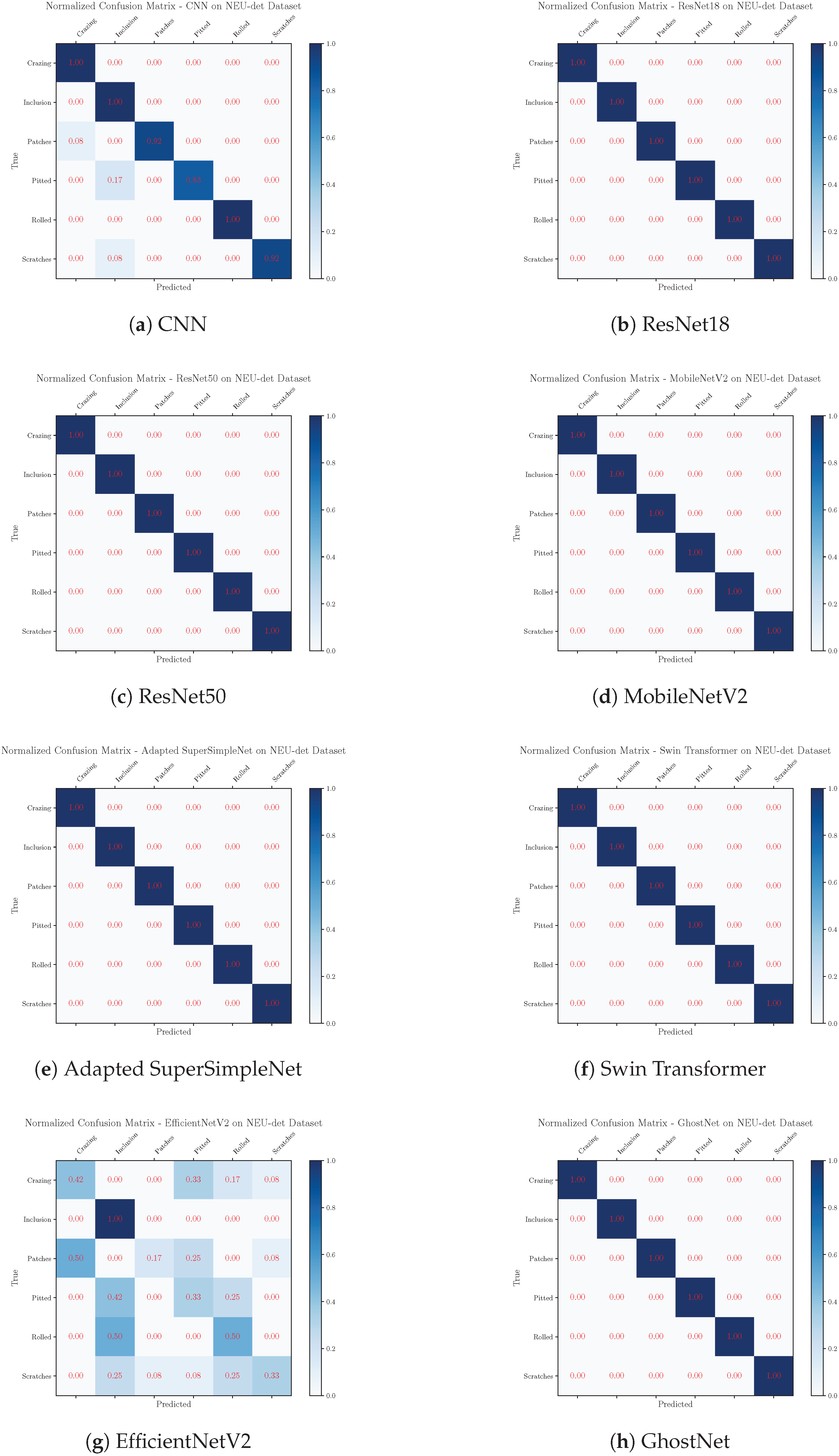
The confusion matrices in Appendix A reveals that the classification errors are not random, but instead follow systematic patterns that are especially visible in the X-SDD dataset. Across multiple architectures, the class “oxide scale of plate system” is repeatedly confused with “slag inclusion” and, in some cases, “red iron”, indicating that these categories likely share similar local texture characteristics and weak inter-class separability under the adopted image-level classification protocol. This tendency is particularly pronounced in lightweight models such as MobileNetV2 and GhostNet, where a substantial fraction of “oxide scale of plate system” samples is classified as “slag inclusion”, suggesting reduced capacity for fine-grained discrimination between visually similar industrial textures. By contrast, stronger convolutional models, such as ResNet50, and Adapted SuperSimpleNet preserve substantially cleaner decision boundaries for these categories. Different failure modes are observed for EfficientNetV2 and the adapted YOLOv12 classifier. Their confusion matrices indicate broader class-collapse behaviour, with several X-SDD categories being absorbed into a small number of dominant predictions, rather than exhibiting only pairwise confusion. These results suggest that architectural efficiency alone is insufficient for robust defect classification when inter-class differences depend on subtle, localized texture features.

Our findings indicate a trade-off between model complexity, performance, and computational efficiency. ResNet50 remains a strong choice for accuracy, while ResNet18 provides a balanced compromise. MobileNetV2, GhostNet, and the Adapted SuperSimpleNet excel in efficiency with low-latency inference, making them ideal for scenarios with constrained resources. Meanwhile, attention-based architectures such as Swin Transformer and CoAtNet confirm the added value of hybrid and transformer-based designs for capturing subtle defect features while still maintaining feasible inference speeds.

Our findings directly translate to automated quality control in manufacturing environments. High-capacity models such as Swin Transformer and CoAtNet are best suited for centralized inspection systems equipped with strong computational resources (e.g., dedicated GPU servers), as required in sectors like automotive steel or aerospace alloy production where detecting subtle, safety-critical defects is paramount. In contrast, lightweight models such as MobileNetV2, GhostNet, and the Adapted SuperSimpleNet are highly suitable for deployment on edge devices (e.g., NVIDIA Jetson modules, industrial PCs) or embedded systems, enabling real-time inspection in continuous processes such as steel coil rolling, welding seams, or magnetic tile profiling.

By explicitly quantifying the trade-offs between accuracy, computational efficiency, and robustness, this study provides actionable guidelines for selecting defect detection models tailored to specific industrial needs. Furthermore, while transformer-based models may require centralized training on high-performance hardware, lightweight CNNs can be trained and fine-tuned even on mid-range GPUs, making them more feasible for widespread adoption. This balance between centralized high-capacity models and deployable lightweight networks strengthens the path toward practical, scalable, and cost-effective industrial defect inspection.

• Centralized inspection: High-capacity models (e.g., Swin Transformer, CoAtNet) are suited for offline or lab environments with server-grade GPUs, enabling detection of subtle and safety-critical defects in demanding industries.
• Edge deployment: Lightweight models (e.g., MobileNetV2, GhostNet, SuperSimpleNet) can run on embedded devices and industrial PCs, supporting real-time inspection in continuous processes.
• Hardware feasibility: Transformer-based models require powerful GPU clusters for training, whereas lightweight CNNs can be trained and fine-tuned on mid-range GPUs, reducing cost barriers.
• Cost–performance trade-off: Clear guidelines are provided to balance accuracy, efficiency, and robustness, helping manufacturers select models aligned with their operational constraints.
• Scalability: Combining centralized training of large models with on-site deployment of lightweight ones enables a practical and scalable inspection strategy for industry.

It should also be noted that all architectures were trained under a unified optimization pipeline, with a common optimizer, learning rate, batch size, and stopping criterion. Although this choice improves fairness and reproducibility in cross-model benchmarking, it may disadvantage architectures that are more sensitive to training dynamics, particularly Transformer-based models such as Swin Transformer and CoAtNet, which often benefit from dedicated learning-rate schedules, warm-up phases, and larger batch sizes. Therefore, the results reported here should be interpreted as performance under a standardized industrial-style baseline protocol rather than as the maximally tuned performance of each architecture.

Transfer learning and domain adaptation are likely to play an important role in the practical robustness of defect classification systems under changing industrial conditions. Transfer learning can improve convergence and reduce the amount of labelled data required by providing pre-trained low-level and mid-level visual representations. However, its effectiveness depends strongly on the similarity between the source domain and the target inspection domain. When substantial shifts occur in lighting conditions, sensor noise, material appearance, surface texture, or imaging setup, the direct transfer of features learned from generic datasets may become less reliable. In such cases, domain adaptation offers a more suitable mechanism to improve resilience, as it can help align feature distributions across different acquisition environments and reduce the performance degradation caused by domain shift.

6. Conclusions

This study presented a systematic and unified evaluation of ten state-of-the-art deep learning architectures, spanning traditional convolutional networks, lightweight CNNs, hybrid CNN–Transformer models, and vision transformers, across five benchmark datasets for surface defect classification. By training and testing all models under consistent experimental conditions, this study provides a rigorous cross-architecture comparison that has been lacking in the literature. Evaluation metrics included accuracy, precision, recall, F1-score, training and execution time, enabling a balanced analysis of both predictive performance and deployment feasibility.

The results highlighted that Swin Transformer and CoAtNet achieve best overall performance in classification, particularly on complex datasets, confirming the value of attention-based mechanisms and hybrid designs for capturing subtle industrial defect patterns. ResNet50 validated the continued strength of deep residual learning, whereas ResNet18 offered a strong compromise between performance and training efficiency. On the lightweight spectrum, MobileNetV2, GhostNet, and the Adapted SuperSimpleNet demonstrated remarkable efficiency-to-accuracy trade-offs, making them well-suited for real-time or embedded deployment on production lines. In contrast, EfficientNetV2 and YOLOv12, despite their promise in other domains, showed weaker generalization in this industrial context, underscoring the importance of domain-specific benchmarking.

The novelty of this study lies in its comprehensive, cross-model evaluation framework, covering a diverse set of modern architectures and benchmarking them across multiple defect datasets using consistent protocols. Unlike prior studies that typically focus on one or two models or a single dataset, the current study establishes a broader and fair performance baseline while explicitly analyzing the trade-offs between accuracy, computational complexity, training time and per-image inference speed. Therefore, this systematic approach bridges the gap between research-driven accuracy benchmarks and industry-driven requirements such as inference speed and resource constraints. By explicitly quantifying these trade-offs, this study provides actionable insights for industry adoption, supporting the reliable deployment of deep learning models in manufacturing environments where efficiency, robustness, and scalability are as critical as accuracy.

Future work should extend this framework to include more diverse and challenging industrial datasets, including those with larger scale, higher resolution, and greater variability in defect types. Larger datasets would provide a more reliable basis for model comparison by reducing sampling bias and improving the statistical robustness of the reported results. Higher-resolution imagery would help preserve fine-grained defect details that may be lost under aggressive resizing, which is particularly relevant for subtle or low-contrast anomalies. In addition, a broader diversity of defect types, surface textures, illumination conditions, and industrial scenarios would allow a more realistic evaluation of model generalization and deployment readiness. Such benchmarks would be especially valuable for assessing whether architectures with stronger multi-scale feature extraction or localization capabilities can better exploit richer visual information in complex real-world inspection tasks. Another important direction is testing and optimizing the evaluated models on real-time edge hardware like industrial computers or embedded systems. This is important to validate deployment feasibility under realistic production constraints. In addition, research into domain adaptation and transfer learning will be valuable for improving robustness across varying conditions such as illumination, noise, and material variability, while temporal inspection of video or time-series data may further capture defect evolution in real time.

Future research should also investigate the extent to which domain adaptation and transfer learning can improve generalization across heterogeneous industrial environments. In particular, it would be valuable to evaluate models under controlled variations in illumination, noise, material properties, and acquisition conditions, in order to quantify their sensitivity to realistic deployment shifts. Comparative studies could also assess whether adaptation strategies, such as fine-tuning across domains, feature-alignment methods, or unsupervised domain adaptation, provide measurable gains over standard transfer learning alone. Such analyses would help determine which architectures are inherently more robust and which require explicit adaptation mechanisms to maintain reliable defect recognition in real-world manufacturing settings.

In summary, this study delivers the first comprehensive and consistent benchmark of diverse deep learning models for surface defect classification, providing both a scientific reference for future research and actionable guidance for industrial deployment.