A Novel Three-Parameter Grey Model with Background Value Optimization and Its Application in Energy Consumption Forecasting

Abstract

Against the backdrop of sustained growth in energy demand and energy transformation in China, accurately predicting future energy consumption trends is essential to developing science-based energy strategies and ensuring energy security. Traditional grey models suffer from limited prediction accuracy due to irrational background value settings. To address this issue, we introduced a structural optimization by adjusting the parameter count within the background value and employed the Simpson formula to reconstruct it. We proposed a novel three-parameter background value grey model, designated as TPBSVGM(1,1). It utilized the annual consumption data of petroleum, natural gas, and primary electricity and other energy consumption from 2014 to 2023 to construct TPBSVGM(1,1) for energy consumption analysis. To assess the predictive accuracy of TPBSVGM(1,1), this study compared its performance with GM(1,1) and FGM(1,1) in two dimensions: the trends between predicted values and actual values, and error metrics. The results indicate that TPBSVGM(1,1) outperforms the comparative models in energy consumption forecasting. We further used the model to predict annual consumption of the three energy sources from 2024 to 2030, finding that total consumption continues to grow while growth rates decline to varying degrees. It provides reliable data support for China’s energy consumption regulation and energy structure optimization.

1. Introduction

Energy is the power source that ensures the quality of production and life and promotes social and economic development [1]. Economic growth is heavily reliant on energy consumption, which not only directly generates carbon dioxide emissions but also influences them through its scale and composition [2]. Carbon dioxide from energy consumption exacerbates global climate change and threatens sustainable development [3]. As a leading energy-consuming and carbon-emitting nation globally, China places significant emphasis on the environmental impacts of carbon discharges and proactively participates in global climate governance [4]. Against this background, China proposes to strive to achieve the “double carbon” goal of “reaching carbon peak in 2030 and carbon neutrality in 2060” [5,6]. In recent years, driven by climate change and “double carbon” goals, China’s energy structure is systematically transforming from high-carbon fossil energy to clean energy [7,8]. The transformation of energy consumption structure is an essential factor affecting the advancement in the low-carbon economy [9]. Furthermore, accurately predicting energy consumption trends serves as a foundation to support optimizing energy strategic layout and ensuring energy security. It is important for China’s energy transformation and global supply chain reshaping. Therefore, the forecasting of energy consumption has attracted considerable interest from the academic community.

At present, researchers mainly focus on artificial intelligence models and statistical approaches to forecast energy consumption. For instance, Wang et al. [10] utilized the LSTM to forecast energy consumption in cold storage refrigeration systems. Wu et al. [11] introduced an energy-consumption-predictive approach grounded in the LSTM. Uzun et al. [12] proposed a forecasting method for energy usage utilizing LSTM and verified its effectiveness. In addition to LSTM neural networks, several studies have adopted k-NN [13], BP-LEAP [14], NNAR [15], ML [16], Stride-TCN [17], and other artificial intelligence models or algorithms to predict energy consumption. Moreover, some studies have applied different data processing and analysis methods to build statistical models to predict energy consumption, such as the literature [18,19].

However, artificial intelligence and statistical models usually require extensive sample data for training [20]. Specifically, artificial intelligence models are prone to overfitting due to gradient anomalies when data volume is insufficient [21]. Statistical models exhibit increased variance in parameter estimation under small sample conditions, which easily leads to hypothesis testing failure [22]. Meanwhile, statistical models typically necessitate assumptions regarding the distribution and linkages of previous data, placing greater reliance on prior findings [23]. Thus, it is urgently necessary to introduce a forecasting approach capable of conducting modeling under limited data and delivering greater effectiveness for energy consumption. In contrast, the grey model has obvious benefits in the modeling mechanism, calculation operation, and short-term prediction.

Deng proposed a grey model to address the shortcomings associated with limited data and poor information [24]. The grey model has gained widespread application due to its straightforward calculation, easy understanding, and relatively excellent prediction accuracy [25]. GM(1,1) represents a fundamental form of grey modeling, which serializes irregular information and reduces the randomness of the initial dataset [26]. However, the background value of traditional grey models is close to the mean, and its smoothness is easily affected by the extreme values of the modeling sequence, resulting in poor smoothness of the background value [27]. To tackle this issue, academics have proposed a range of optimization methods aimed at improving the model’s predictive accuracy. For example, Liu et al. [28] reconstructed the grey model’s background values using the composite integral median theorem, constructing OFAGM(1,1). Zhang et al. [29] employed a background value reconstruction method combining intelligent trapezoidal weights with variable weights, utilizing a genetic algorithm to find the model’s parameter values. In addition, numerous findings have enhanced the two-parameter background values of the grey model, such as the literature [30,31,32].

The improvement of the two-parameter background value enhances the grey model’s prediction accuracy to some extent, while its smoothness remains relatively low. Therefore, researchers have increased the number of background value parameters to mitigate the impact of outliers on the prediction effect, thereby further enhancing the model’s prediction accuracy. For instance, Li et al. [33] proposed a novel three-parameter discrete grey model TDGM(1,1,z,r(R)) from the perspective of background value optimization. Sun et al. [34] designed a dynamically adjustable three-parameter background value grey model, enhancing the model’s predictive performance. Zhu et al. [35] enhanced the accumulation order and background value utilizing the NENG(1,1,k) model, proposing FBNENGM(1,1,k). In addition, some studies have also enhanced the grey model by considering three-parameter background values, such as the literature [36,37,38].

In addition to improving the grey model’s background value, Wu et al. [39] elaborated on the view that Simpson’s equation can improve the reliability of background value calculation by effectively approximating the function integral. Therefore, researchers have extensively discussed improving grey models around this method. Ma et al. [40] incorporated the Simpson equation into GM(1,1), established GM(SD)(1,1), and applied it to forecast GDP and freight volume in Lanzhou. Li et al. [41] mined the initial information utilizing an adaptive accumulating sequence, introduced the Simpson equation into the background value, and proposed MFCSNGBM(1,1). Li et al. [42] developed SISGM(1,1), which employed the Simpson equation to rebuild the background value and utilized the ISRU activation function to modify the initial conditions. Meanwhile, the grey model of background value reconstructed by the Simpson formula is widely used in energy consumption [39], electric vehicle consumption forecast [43], and other fields. These studies promote the mathematical rigor of grey system theory and provide new solutions to small-sample and high-precision prediction problems in practical projects.

However, the research findings of introducing Simpson’s formula into the three-parameter background value grey model are scarce. Traditional three-parameter grey models commonly use low-order numerical integration methods to construct background values, such as the trapezoid formula. This method has only first-order algebraic accuracy and can only integrate linear functions accurately. When applied to nonlinear functions, it introduces truncation error. This error reduces the smoothness of the background value sequence and the model’s predictive accuracy, making it difficult to fully exploit the three-parameter grey model’s nonlinear fitting advantage. Considering that the nonlinear trend described by the three-parameter background value grey model can be approximated by a quadratic function locally, the background value calculation requires at least second-order algebraic accuracy to ensure accurate integration. The Simpson formula has third-order algebraic accuracy and can achieve accurate integration for polynomials of degree three or less.

Therefore, introducing the Simpson formula into the three-parameter model can achieve an accurate match between the numerical integration method and the theoretical order of the model, thereby eliminating the systematic error caused by the background value construction. Furthermore, the Simpson formula approximates the integration interval using three-point quadratic interpolation, thereby improving the smoothness of the background value sequence and enhancing the robustness of the grey model in complex data scenarios. Thus, this study introduced the Simpson formula into the three-parameter background value grey model and proposed a novel variant of this model, referred to as TPBSVGM(1,1).

To validate the prediction accuracy of TPBSVGM(1,1), we utilized annual consumption values for petroleum, natural gas, primary electricity and other energy sources in China as experimental subjects. The experiments employed GM(1,1) and FGM(1,1) as a comparison to test the performance of TPBSVGM(1,1) in forecasting energy consumption. Based on verifying this model’s performance, this study applied TPBSVGM(1,1) to forecast the annual consumption data of three energy sources from 2024 to 2030. This approach aims to clarify the dynamic changes and growth rate trends concerning China’s energy consumption.

The core contributions are outlined as follows:

(1) This study innovatively introduces the Simpson formula into the grey model, expanding the parameter count within the background value, thereby proposing a new grey TPBSVGM(1,1) model. This model enhances the background value series’ smoothness and weakens extreme values’ influence on predictive performance, effectively improving prediction accuracy. Furthermore, this research introduces a novel modeling approach for optimizing the background value of grey models.

(2) This study constructs a TPBSVGM(1,1) model for energy consumption based on China’s annual consumption data of three energy sources from 2014 to 2023. It conducts experimental prediction research to validate the model’s performance. The experiment’s findings demonstrate that TPBSVGM(1,1) outperforms comparison models in forecasting energy consumption, achieving an “excellent” level of accuracy. Therefore, this research offers a novel predictive methodology for energy consumption.

(3) This study employs the proposed TPBSVGM(1,1) to forecast and analyze the annual data of the aforementioned three energy consumption categories from 2024 to 2030. This approach elucidates the dynamic changes and increasing rate trends in China’s energy consumption. The findings of this study offer essential data to the energy sector and facilitate the transformation in its energy structure. Furthermore, these results offer a scientific foundation for global climate governance, which is crucial for advancing reforms in the global energy governance system.

This study’s remaining organizational structure is as follows: Section 2 explains the modeling principles, steps, the comparison method for the smoothness of background value sequences, and criteria for judging model accuracy of TPBSVGM(1,1). Section 3 conducts experimental prediction studies on the consumption of petroleum, natural gas, primary electricity and other energy, respectively, thereby verifying the prediction accuracy of TPBSVGM(1,1) in energy consumption. Furthermore, this section uses TPBSVGM(1,1) to forecast the three types of energy consumption from 2024 to 2030, thereby analyzing the dynamic evolution and increasing rate trend of energy consumption. Section 4 is the main conclusion.

2. Materials and Methods

2.1. TPBSVGM(1,1)

The background value of GM(1,1) is close to the mean value, and its smoothness is easily affected by the extreme data of the modeling sequence. Consequently, it has poor smoothness. However, the background value’s smoothness substantially influences prediction accuracy. In other words, the higher the smoothness, the better the prediction effect. Generally, the smoothness of three-parameter background values is higher than that of two-parameter background values. To improve the ability to cope with smooth mutations, this study uses the Simpson formula to construct background values and introduces a novel TPBSVGM(1,1) model. The methodology for modeling is outlined below.

Step 1: The initial dataset is $H^{(0)}=\left\{h^{(0)}(1),h^{(0)}(2),\dots ,h^{(0)}(n)\right\}$. The first-order accumulation sequence of $H^{(0)}$ is $H^{(1)}$, $H^{(1)}=\left\{h^{(1)}(1),h^{(1)}(2),\dots ,h^{(1)}(n)\right\}$, where $h^{(1)}\left(t\right)={\displaystyle \sum _{t=1}^n{h}^{(0)}\left(t\right),\left(t=1,2,3,\dots ,n\right)}$.

Step 2: Build the equation

$$h^{\left(0\right)}\left(t\right)+{\displaystyle \frac{1}{6}}\alpha \left(h^{\left(1\right)}\left(t\right)+4h^{\left(1\right)}\left(t-1\right)+h^{\left(1\right)}\left(t-2\right)\right)=t\beta +\gamma$$

(1)

The parameters $\alpha$ and $\beta$ are development coefficients, and $\gamma$ is the grey action quantity.

Step 3: Calculating parameters by the least squares approach

$$\widehat{\mathrm{u}}={\left(\alpha ,\beta ,\gamma \right)}^{\mathrm{{\rm T}}}={\left(P^{\mathrm{{\rm T}}}P\right)}^{-1}{P}^{\mathrm{{\rm T}}}Q$$

where the matrices $P$ and $Q$ are defined as follows:

$$P=\left[\begin{array}{ccc}-{\displaystyle \frac{1}{6}}\left(h^{\left(1\right)}\left(3\right)+4h^{\left(1\right)}\left(2\right)+h^{\left(1\right)}\left(1\right)\right)& 3& 1\\ -{\displaystyle \frac{1}{6}}\left(h^{\left(1\right)}\left(4\right)+4h^{\left(1\right)}\left(3\right)+h^{\left(1\right)}\left(2\right)\right)& 4& 1\\ ⋮& ⋮& ⋮\\ -{\displaystyle \frac{1}{6}}\left(h^{\left(1\right)}\left(n\right)+4h^{\left(1\right)}\left(n-1\right)+h^{\left(1\right)}\left(n-2\right)\right)& n& 1\end{array}\right],Q=\left[\begin{array}{c}{h}^{\left(0\right)}\left(3\right)\\ h^{\left(0\right)}\left(4\right)\\ ⋮\\ h^{\left(0\right)}\left(n\right)\end{array}\right]$$

Step 4: Solve the equation

According to Step 1:

$${\widehat{h}}^{\left(0\right)}\left(t\right)={\widehat{h}}^{\left(1\right)}\left(t\right)-{\widehat{h}}^{\left(1\right)}\left(t-1\right),t=3,4,\dots ,n$$

(2)

Substituting Equation (2) into Equation (1), we get

$${\widehat{h}}^{\left(1\right)}\left(t\right)-{\widehat{h}}^{\left(1\right)}\left(t-1\right)+{\displaystyle \frac{1}{6}}\alpha \left(h^{\left(1\right)}\left(t\right)+4h^{\left(1\right)}\left(t-1\right)+h^{\left(1\right)}\left(t-2\right)\right)=t\beta +\gamma$$

Get

$$\left(1+{\displaystyle \frac{1}{6}}\alpha \right){\widehat{h}}^{\left(1\right)}\left(t\right)-\left(1-{\displaystyle \frac{2}{3}}\alpha \right){\widehat{h}}^{\left(1\right)}\left(t-1\right)+{\displaystyle \frac{\alpha }{6}}{\widehat{h}}^{\left(1\right)}\left(t-2\right)=t\beta +\gamma$$

Sort the expression to get

$${\widehat{h}}^{\left(1\right)}\left(t\right)={\displaystyle \frac{6-4\alpha }{6+\alpha }}{\widehat{h}}^{\left(1\right)}\left(t-1\right)-{\displaystyle \frac{\alpha }{6+\alpha }}{\widehat{h}}^{\left(1\right)}\left(t-2\right)+{\displaystyle \frac{6\beta }{6+\alpha }}t+{\displaystyle \frac{6\gamma }{6+\alpha }}$$

Let

$${\delta }_1={\displaystyle \frac{6-4\alpha }{6+\alpha }},{\delta }_2=-{\displaystyle \frac{\alpha }{6+\alpha }},{\delta }_3={\displaystyle \frac{6\beta }{6+\alpha }},{\delta }_4={\displaystyle \frac{6\gamma }{6+\alpha }}$$

Get

$${\widehat{h}}^{\left(1\right)}\left(t\right)={\delta }_1{\widehat{h}}^{\left(1\right)}\left(t-1\right)+{\delta }_2{\widehat{h}}^{\left(1\right)}\left(t-2\right)+{\delta }_{3}t+{\delta }_4$$

(3)

Bring Formula (3) into Formula (2) and get the final recovery expression as follows:

$${\widehat{h}}^{\left(0\right)}\left(t\right)={\delta }_1{\widehat{h}}^{\left(1\right)}\left(t-1\right)+\left({\delta }_2-{\delta }_1\right){\widehat{h}}^{\left(1\right)}\left(t-2\right)-{\delta }_2{\widehat{h}}^{\left(1\right)}\left(t-3\right)+{\delta }_3$$

It can be seen that the time-response function of TPBSVGM(1,1) is a recursive function; the predicted value ${\widehat{h}}^{\left(0\right)}\left(t\right)$ at the current moment is iteratively generated from the cumulative predicted values ${\widehat{h}}^{\left(1\right)}\left(t-1\right)$, ${\widehat{h}}^{\left(1\right)}\left(t-2\right)$, and ${\widehat{h}}^{\left(1\right)}\left(t-3\right)$ at the previous three moments. The above recovery expression is the recursive formula of the model.

Sorting out Formula (3), when $t$ = 3 or 4, we get

$${\widehat{h}}^{\left(1\right)}\left(3\right)={\delta }_1{h}^{\left(1\right)}\left(2\right)+{\delta }_2{h}^{\left(1\right)}\left(1\right)+{\delta }_{3}t+{\delta }_4$$

(4)

$${\widehat{h}}^{\left(1\right)}\left(4\right)={\delta }_1{\widehat{h}}^{\left(1\right)}\left(3\right)+{\delta }_2{h}^{\left(1\right)}\left(2\right)+{\delta }_{3}t+{\delta }_4$$

(5)

$h^{\left(1\right)}\left(1\right)$ and $h^{\left(1\right)}\left(2\right)$ are the initial values for the TPBSVGM(1,1), and these two values are known.

By introducing Formula (4) into Formula (5), we can get

$${\widehat{h}}^{\left(1\right)}\left(4\right)=\left({\delta }_1{}^2+{\delta }_2\right){\widehat{h}}^{\left(1\right)}\left(2\right)+{\delta }_1{\delta }_2{\widehat{h}}^{\left(1\right)}\left(1\right)+3{\delta }_1{\delta }_3+{\delta }_1{\delta }_4+4{\delta }_3+{\delta }_4$$

(6)

When $t=5$, we get

$${\widehat{h}}^{\left(1\right)}\left(5\right)={\delta }_1{\widehat{h}}^{\left(1\right)}\left(4\right)+{\delta }_2{\widehat{h}}^{\left(1\right)}\left(3\right)+5{\delta }_3+{\delta }_4$$

(7)

By introducing Formula (6) into Formula (7), we can get

$$\begin{array}{l}{\widehat{h}}^{\left(1\right)}\left(5\right)=\left({\delta }_1{}^3+2{\delta }_1{\delta }_2\right)h^{\left(1\right)}\left(2\right)+\left({\delta }_1{}^2{\delta }_2+{\delta }_2{}^2\right)h^{\left(1\right)}\left(1\right)+3{\delta }_1{}^2{\delta }_3+{\delta }_1{}^2{\delta }_4+\\ \hspace{1em}\hspace{1em}\hspace{1em}4{\delta }_1{\delta }_3+{\delta }_1{\delta }_4+3{\delta }_2{\delta }_3+{\delta }_2{\delta }_4+5{\delta }_3+{\delta }_4\end{array}$$

Similarly, when $t=6$, we get

$${\widehat{h}}^{\left(1\right)}\left(6\right)={\delta }_1{\widehat{h}}^{\left(1\right)}\left(5\right)+{\delta }_2{\widehat{h}}^{\left(1\right)}\left(4\right)+6{\delta }_3+{\delta }_4$$

Repeating the above steps, we get

$$\begin{array}{cc}\hfill {\widehat{h}}^{\left(1\right)}\left(6\right)=& \left({\delta }_1{}^4+3{\delta }_1{}^2{\delta }_2+{\delta }_2{}^2\right)h^{\left(1\right)}\left(2\right)+\left({\delta }_1{}^3{\delta }_2+2{\delta }_1{\delta }_2{}^2\right)h^{\left(1\right)}\left(1\right)+3{\delta }_1{}^3{\delta }_3+{\delta }_1{}^3{\delta }_4+4{\delta }_1{}^2{\delta }_3\hfill \\ \hfill +& {\delta }_1{}^2{\delta }_4+6{\delta }_1{\delta }_2{\delta }_3+2{\delta }_1{\delta }_2{\delta }_4+5{\delta }_1{\delta }_3+{\delta }_1{\delta }_4+4{\delta }_2{\delta }_3+{\delta }_2{\delta }_4+6{\delta }_3+{\delta }_4\hfill \end{array}$$

From the foregoing derivation, we can confirm that the time-response function for TPBSVGM(1,1) corresponds to a recursive function, and the functional expression for the prediction sequence cannot be directly obtained. Thus, we employed MATLAB (R2016a) to develop recursive programs to calculate fitted and predicted values.

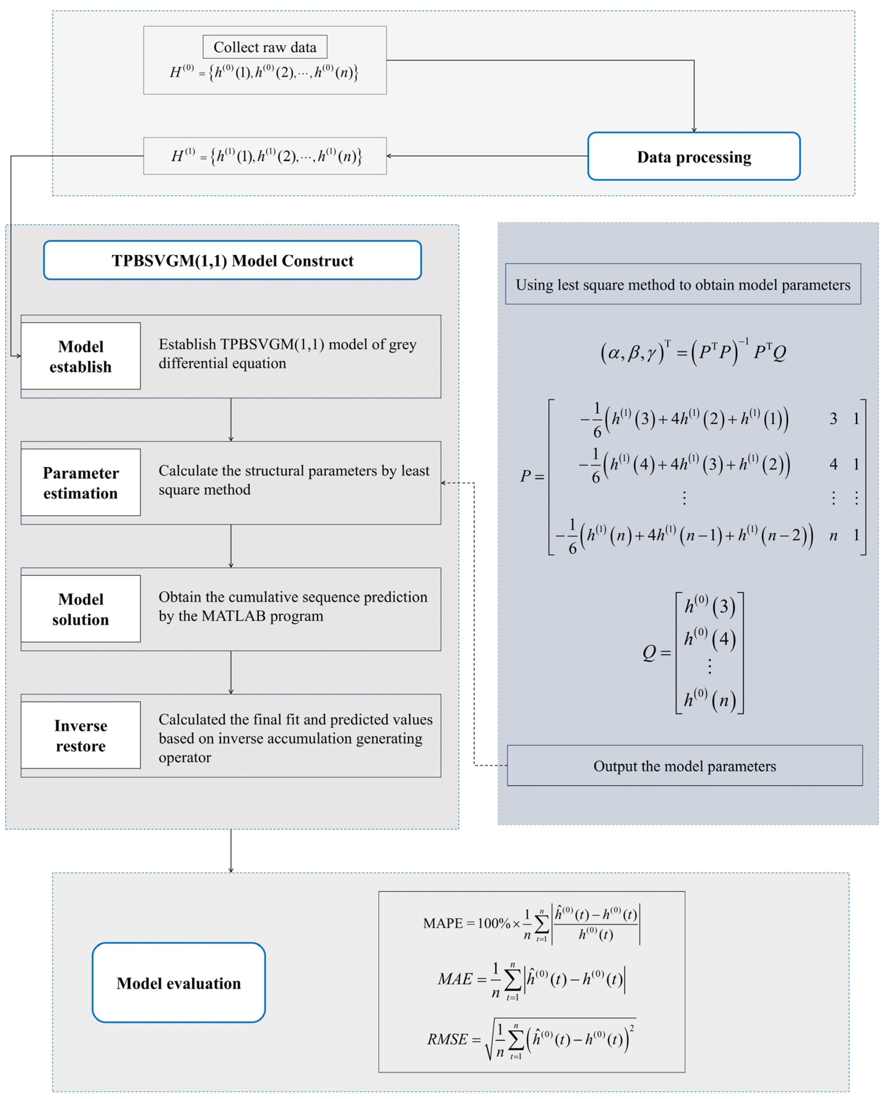
To further reveal the modeling and prediction process of TPBSVGM(1,1), this study presents the data processing, model construction, and evaluation of the model, as depicted in Figure 1.

2.2. Comparison Method for Smoothness of Background Value Sequences

2.2.1. Definition and Calculation Method of Smoothness

This study uses the variance of the first-order difference sequence of the background values as the measure of smoothness. The background value sequence is $Z^{(1)}\left(t\right)$. The first-order difference of the background value sequence is $\Delta z\left(t\right)=z^{\left(1\right)}\left(t\right)-z^{\left(1\right)}\left(t-1\right)$.

The variance of this first-order difference sequence is

$$S=\mathit{Var}\left(\Delta z\left(t\right)\right)$$

(8)

A smaller variance $S$ implies higher smoothness of the background value sequence, whereas a larger variance indicates lower smoothness.

2.2.2. Comparison of Background Value Smoothness in Grey Models

To visually illustrate the differences in background value smoothness across models, this study selects the original sequence $H^{(0)}=\left[5, 6, 9, 11, 12, 16, 27\right]$. After the first-order accumulative generation, we construct the background values for TPBSVGM(1,1), GM(1,1), and FGM(1,1), respectively. Then, we calculate the variance $S$ of their first-order difference sequences by Equation (8).

The background value sequences of GM(1,1) and FGM(1,1) are $Z=\left[8.0, 15.5, 25.5, 37.0, 51.0, 72.5\right]$, and their first-order difference sequences are $\Delta Z=\left[7.5, 10.0, 11.5, 14.0, 21.5\right]$. The corresponding smoothness variance is calculated as $S\approx 28.7$.

The background value sequence of TPBSVGM(1,1) is $Z=\left[8.8, 10.9, 12.5, 17.2\right]$, and its first-order difference sequence is $\Delta Z=\left[8.0, 10.2, 13.0, 16.0\right]$. The corresponding smoothness variance is calculated as $S\approx 12.0$.

It can be seen that the background value smoothness of TPBSVGM(1,1) is significantly higher than that of GM(1,1) and FGM(1,1), thereby verifying the effectiveness of the improvements to the background value construction in TPBSVGM(1,1).

2.3. Accuracy Evaluation Method

This study uses three error indicators to validate the precision of the models, as follows:

$$\mathrm{MAPE}=100\%\times {\displaystyle \frac{1}{n}}{\displaystyle \sum _{t=1}^n\left|\frac{{\widehat{h}}_{}^{(0)}(t)-h^{(0)}(t)}{h^{(0)}(t)}\right|}$$

(9)

$$\mathrm{MAE}={\displaystyle \frac{1}{n}}{\displaystyle \sum _{t=1}^n\left|{\widehat{h}}_{}^{(0)}(t)-h^{(0)}(t)\right|}$$

(10)

$$\mathrm{RMSE}=\sqrt{{\displaystyle \frac{1}{n}}{\displaystyle \sum _{t=1}^n({\widehat{h}}^{(0)}(t)-h^{(0)}(t)}{)}^2}$$

(11)

The MAPE measures the predictive ability of the models. A lower MAPE corresponds to a higher level of prediction accuracy. The assessment criteria are presented in

Table 1. MAPE-based classification for predictive ability [44].

MAPE (%)	Predictive Ability
<10	Excellent
10–20	Relatively good
20–50	General
>50	Poor

.

3. Results and Discussion

3.1. Comparison of Fitting Accuracy Between Different Models

3.1.1. Experiment 1: Petroleum Consumption Forecast

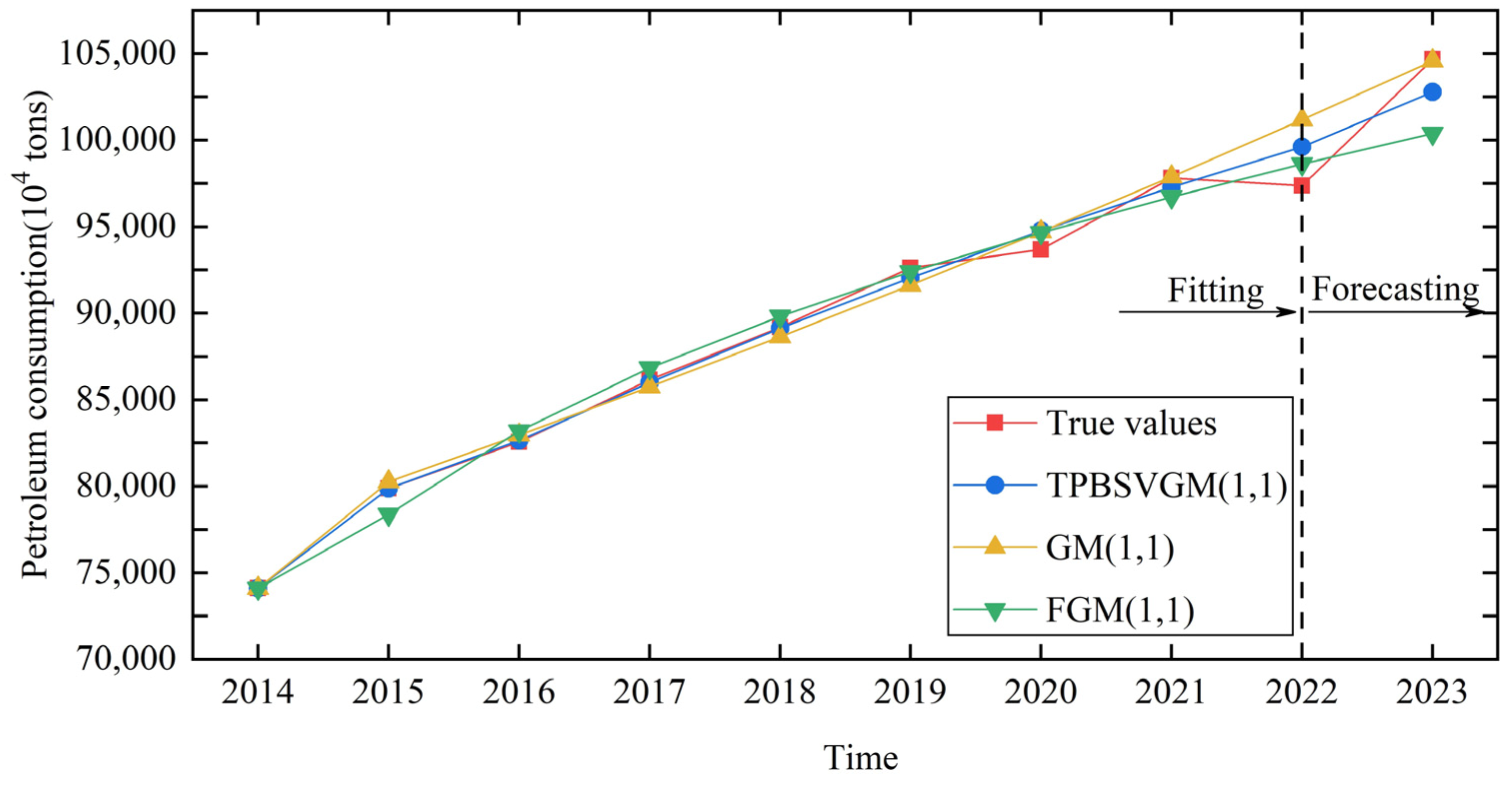
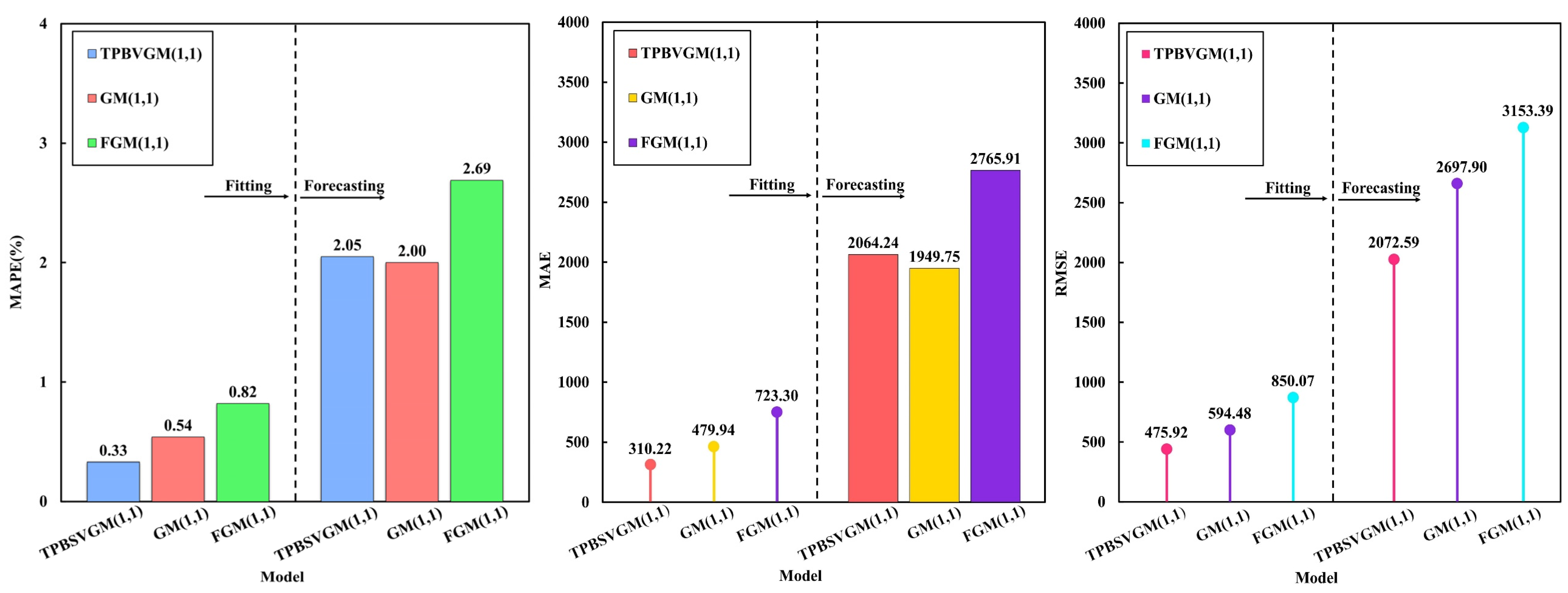
Experiment 1 focuses on annual petroleum consumption data for prediction research. This study selected annual petroleum consumption data from 2014 to 2023, including 10 years of data (from https://www.stats.gov.cn/sj/ndsj/, accessed on 24 March 2025). We divided the data according to a ratio of 8:2. The petroleum consumption data from 2014 to 2021 were used to construct TPBSVGM(1,1) and its comparison models. The data from 2022 to 2023 were then employed to evaluate the predictive capability of these models. The modeling and test data of the total petroleum consumption on each model are shown in

Table 2. Modeling and test data for Experiment 1. Unit: 10⁴ tons.

Year	True Value	TPBSVGM(1,1)		GM(1,1)		FGM(1,1)
		Value	APE (%)	Value	APE (%)	Value	APE (%)
In-sample (fitting)
2014	74,101.78	74,101.78	0.00	74,101.78	0.00	74,101.78	0.00
2015	79,876.79	79,876.79	0.00	80,264.43	0.49	78,371.61	1.88
2016	82,559.00	82,638.35	0.10	82,964.92	0.49	83,201.60	0.78
2017	86,151.30	85,995.00	0.18	85,756.27	0.46	86,848.96	0.81
2018	89,193.83	89,133.79	0.07	88,641.53	0.62	89,831.65	0.72
2019	92,622.72	92,051.06	0.62	91,623.86	1.08	92,393.31	0.23
2020	93,683.03	94,762.01	1.15	94,706.54	1.09	94,664.92	1.05
2021	97,816.66	97,281.22	0.55	97,892.94	0.08	96,724.82	1.12
MAPE (%)		0.33		0.54		0.82
MAE		310.22		479.94		723.30
RMSE		475.92		594.48		850.07
Out-of-sample (forecasting)
2022	97,372.08	99,622.24	2.31	101,186.54	3.92	98,623.54	1.29
2023	104,676.00	102,797.69	1.79	104,590.95	0.08	100,395.63	4.09
MAPE (%)		2.05		2.00		2.69
MAE		2064.24		1949.75		2765.91
RMSE		2072.59		2697.90		3153.39

. To more intuitively present the dynamic change trend between true values and model-predicted values, as well as to compare the three error metrics across models in Experiment 1, this study presents the experimental data with visual means, as shown in Figure 2 and Figure 3.

As shown in Figure 2, during the fitting phase, the predicted values of three models exhibit a comparatively synchronous trend with the true values. In particular, except for the deviation between the predicted value of FGM(1,1) and the actual value in 2015, which is significantly greater than TPBSVGM(1,1) and GM(1,1), the predicted and actual values for the three models show approximate overlap in most years. In the forecasting period, the forecast results of FGM(1,1) in 2022 exhibit the highest consistency with the true data, while the discrepancy is greatest in 2023. The forecasting data for GM(1,1) in 2023 is closest to the true data, while the deviation is most significant in 2022. Therefore, TPBSVGM(1,1) has more stable performance during the prediction phase and minor deviation fluctuations. In summary, compared to the comparison model, the prediction performance of TPBSVGM(1,1) is more stable and adaptable.

To further reveal the differences in prediction accuracy between the above three models, this study compares and analyzes the error indicators of the models in Experiment 1. As illustrated in Figure 3, during the fitting stage, the three error indicators of TPBSVGM(1,1) are smaller than GM(1,1) and FGM(1,1). This indicates that TPBSVGM(1,1) delivers superior predictive ability relative to the latter two models in this stage. During the forecasting stage, the values of the three error indicators for FGM(1,1) are higher than those of TPBSVGM(1,1). The MAPE and RMSE values for GM(1,1) are higher than those of TPBSVGM(1,1), while the MAE value for the former exhibits a marginally lower value relative to TPBSVGM(1,1).

To systematically evaluate the predictive accuracy of TPBSVGM(1,1) and GM(1,1), this study comprehensively analyzes the models’ performance during both the fitting and forecasting phases. The findings indicated that the comprehensive MAE values of TPBSVGM(1,1) and GM(1,1) are 1187.23 and 1214.85, respectively. It demonstrates that TPBSVGM(1,1) has lower errors in the prediction stage. Therefore, by comprehensively comparing the error data among the involved models across both stages, it is evident that the predictive ability of TPBSVGM(1,1) outperforms the two comparative models.

To sum up, analyzing the dynamic trends of prediction data of the above three models and true data, and comparing the error indicators shows that compared with GM(1,1) and FGM(1,1), TPBSVGM(1,1) has higher prediction accuracy.

3.1.2. Experiment 2: Natural Gas Consumption Forecast

Experiment 1 proved the performance of TPBSVGM(1,1) in predicting petroleum consumption. To further validate the efficacy of TPBSVGM(1,1) in predicting energy consumption, Experiment 2 conducts a prediction study using natural gas consumption data. This experiment’s data source and interval division were the same as those for Experiment 1. The prediction methodology employed in Experiment 2 was also consistent with that used in Experiment 1.

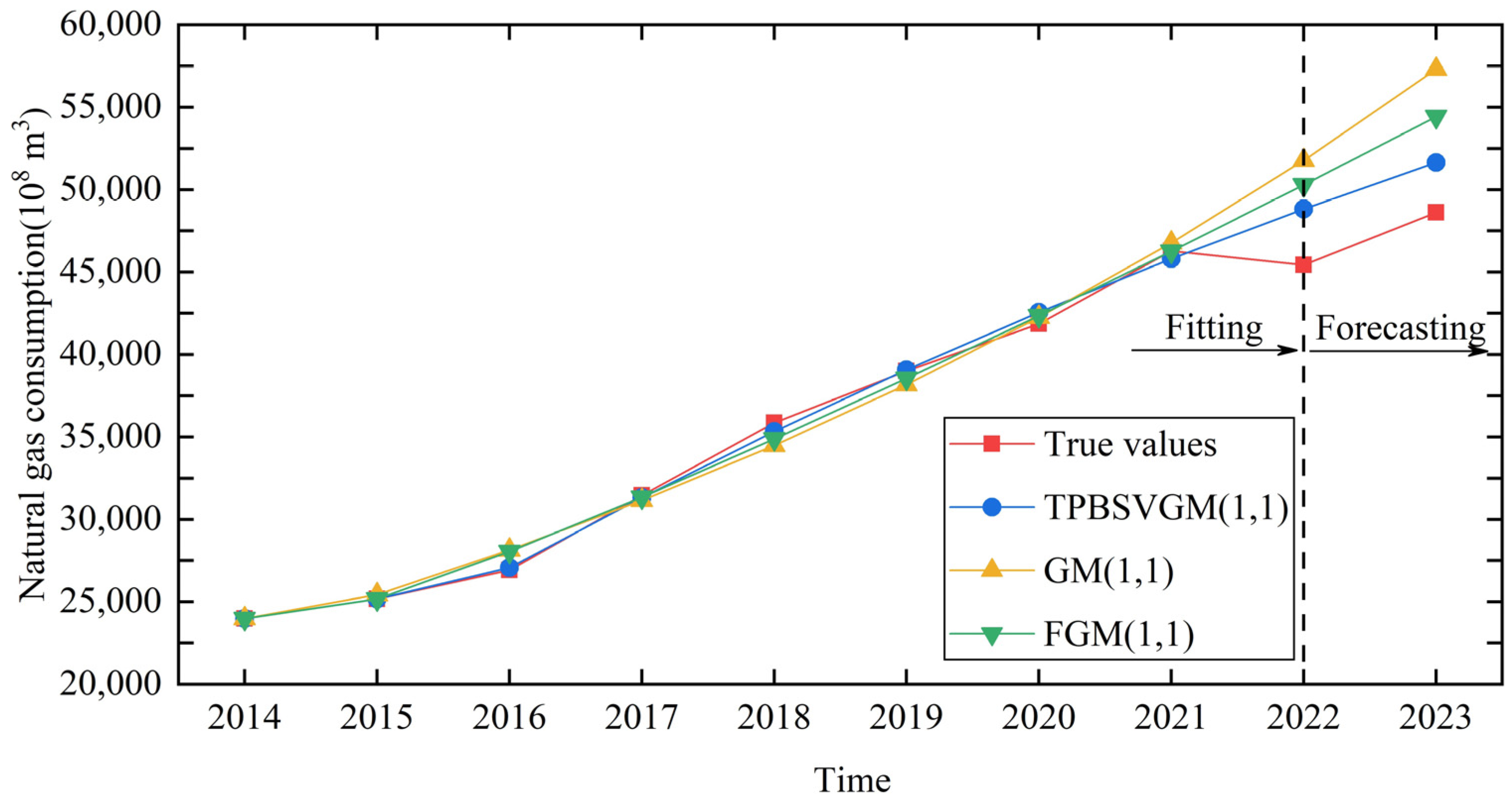
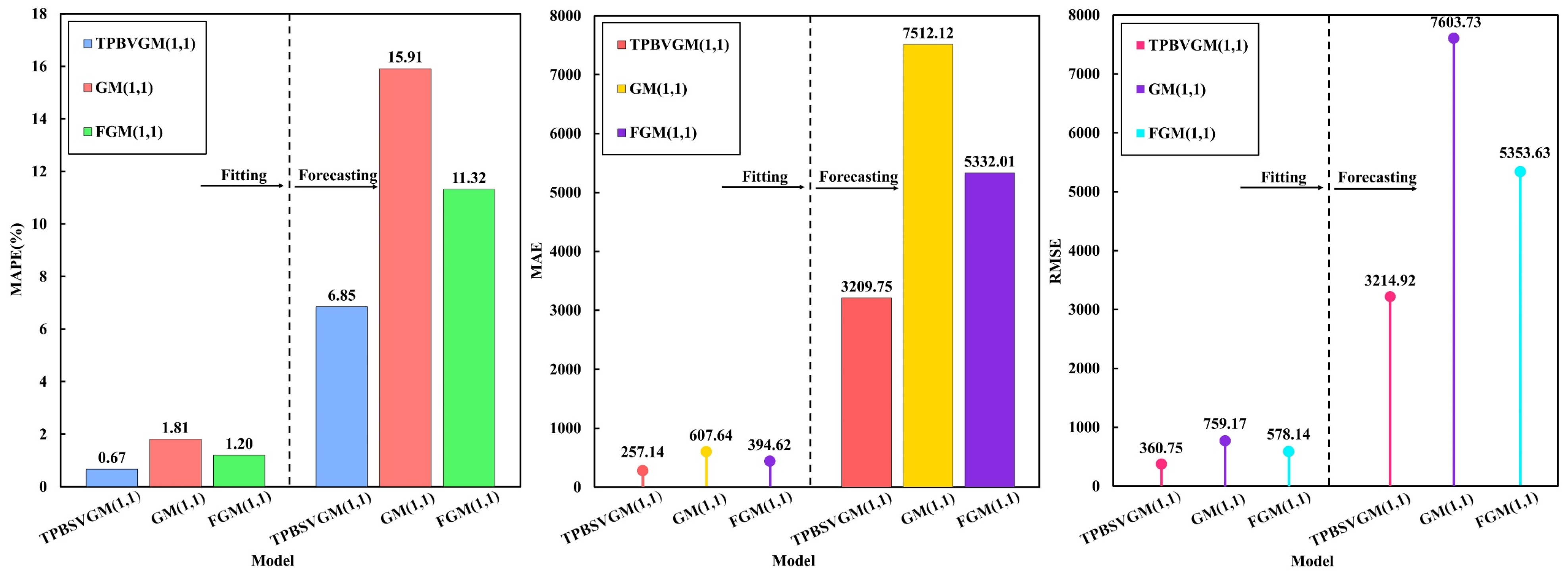
The data acquired in Experiment 2 are presented in

Table 3. Modeling and test data for Experiment 2. Unit: 10⁸ m³.

Year	True Value	TPBSVGM(1,1)		GM(1,1)		FGM(1,1)
		Value	APE (%)	Value	APE (%)	Value	APE (%)
In-sample (fitting)
2014	23,986.70	23,986.70	0.00	23,986.70	0.00	23,986.70	0.00
2015	25,178.55	25,178.55	0.00	25,436.10	1.02	25,178.61	0.00
2016	26,931.01	27,075.37	0.54	28,154.45	4.54	28,046.34	4.14
2017	31,452.06	31,322.92	0.41	31,163.30	0.92	31,353.18	0.31
2018	35,866.30	35,338.42	1.47	34,493.71	3.83	34,877.45	2.76
2019	38,999.04	39,079.73	0.21	38,180.03	2.10	38,551.43	1.15
2020	41,858.38	42,564.29	1.69	42,260.31	0.96	42,350.17	1.17
2021	46,278.85	45,809.68	1.01	46,776.65	1.08	46,264.41	0.03
MAPE (%)		0.67		1.81		1.20
MAE		257.14		607.64		394.62
RMSE		360.75		759.17		578.14
Out-of-sample (forecasting)
2022	45,440.30	48,832.32	7.46	51,775.65	13.94	50,291.64	10.68
2023	48,620.00	51,647.49	6.23	57,308.89	17.87	54,432.68	11.96
MAPE (%)		6.85		15.91		11.32
MAE		3209.75		7512.12		5332.01
RMSE		3214.92		7603.73		5353.63

. Additionally, the trends observed between the predicted and actual data, as well as the comparison trends of the error indicators for the above three models in Experiment 2, are shown in Figure 4 and Figure 5.

As indicated in Figure 4, in the fitting phase, the predicted values for the three models in most years align with the true values. In other words, the predictive data generated by the three models exhibit a high degree of consistency with the actual data for the years 2014, 2015, 2017, 2019, 2020, and 2021. Conversely, the predicted data of the three models and the actual data in 2016 and 2018 show relatively noticeable differences. Furthermore, the predicted data of GM(1,1) and FGM(1,1) in 2016 and 2018 deviate from the actual data relatively more than those of TPBSVGM(1,1). Compared with the other two models, the distinction between the predicted data and the true data of TPBSVGM(1,1) is smaller during the prediction phase. Thus, we can see that the predicted values of TPBSVGM(1,1) have the slightest deviation from the true values, and the change trend between them is more consistent.

To better clarify the differences in natural gas consumption forecasting accuracy among TPBSVGM(1,1), GM(1,1), and FGM(1,1), this study compares and analyzes the error indicators for these three models. As displayed in Figure 5, during the fitting process, the three error indicators of TPBSVGM(1,1) are all the smallest among the three models. During the predictive phase, the three error indicators of TPBSVGM(1,1) exhibit remarkably smaller values relative to the comparison models. Furthermore, in light of this model’s prediction accuracy as measured by the MAPE, the MAPE of TPBSVGM(1,1) is 6.85%, indicating that the prediction performance reaches an “Excellent” level. However, the MAPE for the other two models ranges from 10% to 20%, demonstrating that their prediction accuracy only reaches a “Relatively good” level. Therefore, by comparing the error indicators for the three models in the two stages, it can be observed that the forecasting capability of TPBSVGM(1,1) stands out relative to the other two models.

In conclusion, by comprehensively analyzing the dynamic trends between the predicted and actual data and comparing the error metrics, it follows that TPBSVGM(1,1) exhibits better predictive performance in natural gas consumption prediction compared to the comparative models.

3.1.3. Experiment 3: Primary Electricity and Other Energy Consumption Forecast

Experiments 1 and 2 prove the accuracy of TPBSVGM(1,1) in petroleum and natural gas consumption prediction, respectively. To further verify the models’ prediction performance in energy consumption, Experiment 3 conducted prediction research based on annual consumption data of primary electricity and other energy consumption. The data source and set division selected were consistent with Experiments 1 and 2.

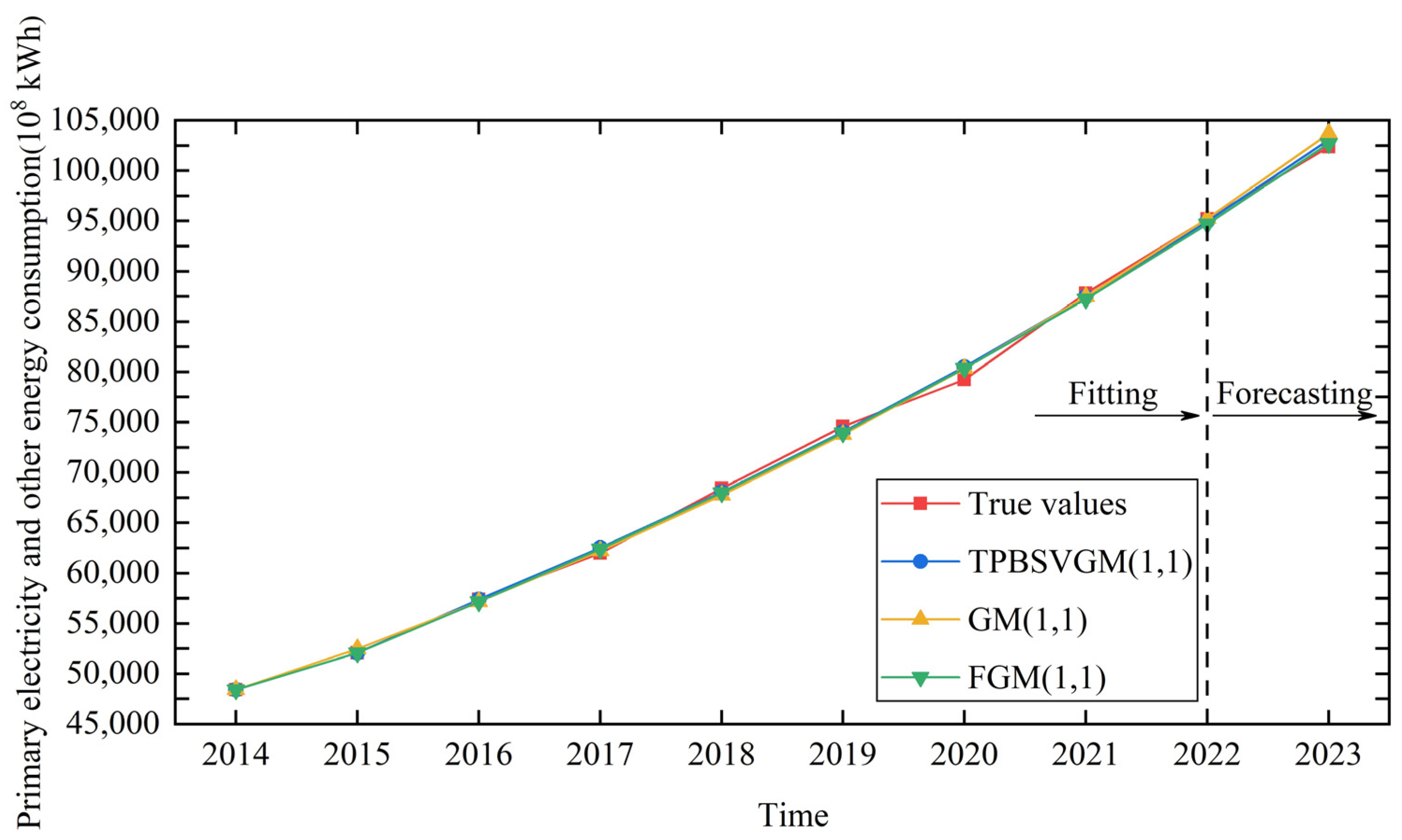
The modeling and calculation ideas for Experiment 3 align with Experiments 1 and 2. The pertinent data obtained from this experiment are shown in

Table 4. Modeling and test data for Experiment 3. Unit: 10⁸ kWh.

Year	True Value	TPBSVGM(1,1)		GM(1,1)		FGM(1,1)
		Value	APE (%)	Value	APE (%)	Value	APE (%)
In-sample (fitting)
2014	48,401.74	48,401.74	0.00	48,401.74	0.00	48,401.74	0.00
2015	52,093.56	52,093.56	0.00	52,487.38	0.76	52,094.67	0.00
2016	57,393.96	57,387.45	0.01	57,150.98	0.42	57,163.51	0.40
2017	61,992.47	62,518.67	0.85	62,228.95	0.38	62,421.27	0.69
2018	68,429.13	68,067.93	0.53	67,758.10	0.98	67,992.62	0.64
2019	74,585.66	74,053.32	0.71	73,778.53	1.08	73,950.76	0.85
2020	79,231.93	80,509.52	1.61	80,333.89	1.39	80,352.11	1.41
2021	87,824.63	87,473.56	0.40	87,471.70	0.40	87,247.61	0.66
MAPE (%)		0.51		0.68		0.58
MAE		381.87		475.79		428.62
RMSE		552.98		582.09		549.82
Out-of-sample (forecasting)
2022	95,208.26	94,985.36	0.23	95,243.72	0.04	94,687.21	0.55
2023	102,388.00	103,088.03	0.68	103,706.29	1.29	102,722.06	0.33
MAPE (%)		0.46		0.66		0.44
MAE		461.46		676.88		427.55
RMSE		519.48		932.51		437.66

. Moreover, Figure 5 and Figure 6 present the trends for both true and forecasted data concerning the consumption of primary electricity and other energy sources. Additionally, these figures provide a comparison of error indicators among the models.

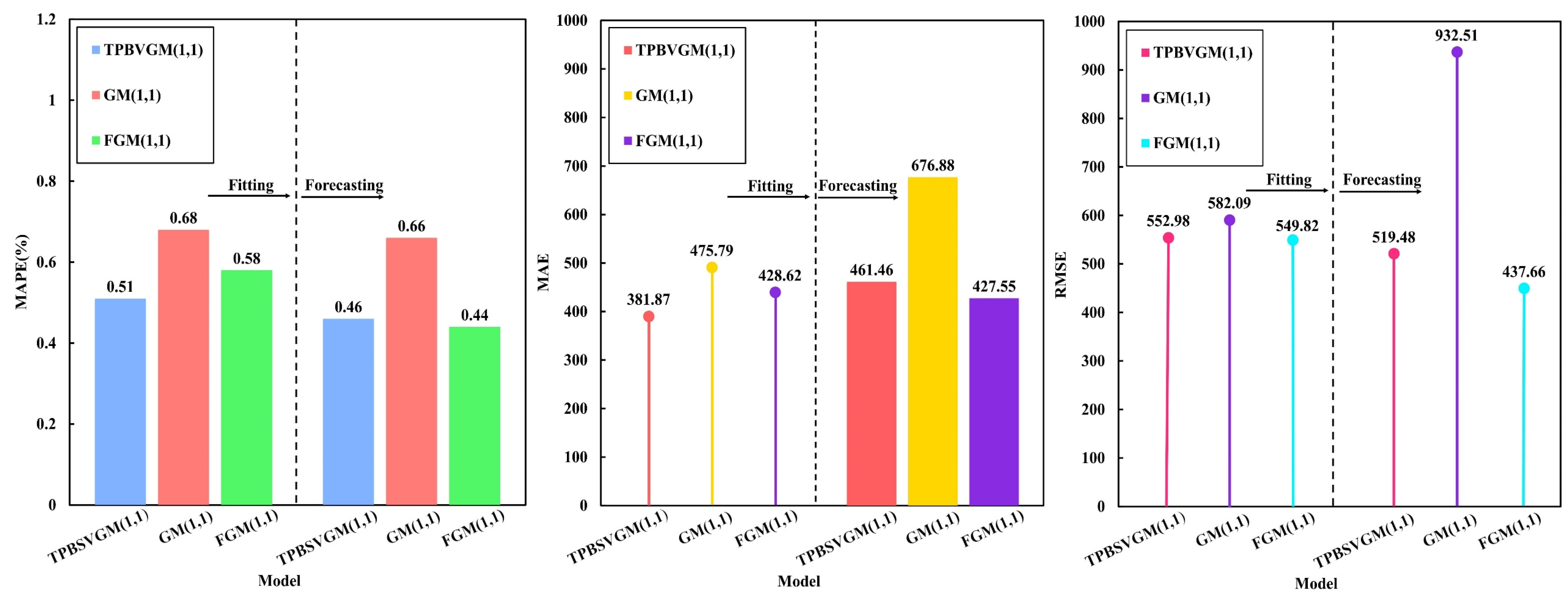
As presented in Figure 6, the trends of the predictive results for TPBSVGM(1,1), GM(1,1), and FGM(1,1) all exhibit a highly synchronous situation during the fitting and prediction stages. To further explore the differences in prediction performance among the three models, this study analyzes the error indicators. As seen in Figure 7, the MAPE of the three models is all less than 1%, and far less than 10%. Based on the MAPE forecasting precision judgment standard, the prediction ability of these three models reached the “Excellent” level in Experiment 3. Further comparison of the MAPE for the three models shows that the MAPE of TPBSVGM(1,1), GM(1,1), and FGM(1,1) during the fitting phase are 0.51%, 0.68%, and 0.58%, respectively. During the prediction phase, their MAPE is 0.46%, 0.66%, and 0.44%, respectively. It is evident that TPBSVGM(1,1) achieves the smallest MAPE in the fitting stage, while FGM(1,1) exhibits the lowest MAPE in the prediction stage.

To further compare the predictive performance of TPBSVGM(1,1) and FGM(1,1), this study comprehensively calculates and obtains the comprehensive MAPE values of the models during the fitting and prediction stages. The comprehensive MAPE is 0.49% for TPBSVGM(1,1) and 0.51% for FGM(1,1). Consequently, the prediction accuracy of TPBSVGM(1,1) outperforms FGM(1,1). In summary, the comparison of MAPE among the three models indicates that the prediction ability of TPBSVGM(1,1) is superior to that of the comparison model.

Combining the MAE of the three models in Figure 7, we find that TPBSVGM(1,1) has the lowest MAE in the fitting phase. However, FGM(1,1) has the lowest MAE during the forecasting stage. Integrating the MAE from both the fitting and forecasting phases, the comprehensive MAE of TPBSVGM(1,1), GM(1,1), and FGM(1,1) are 421.67, 576.34, and 428.09, respectively. Thus, TPBSVGM(1,1) exhibits superior predictive ability than the comparison models. The RMSE in Figure 7 also reveals that TPBSVGM(1,1) in both stages is significantly lower than GM(1,1), but slightly higher than FGM(1,1).

Overall, by systematically comparing the errors for the three models, we find that TPBSVGM(1,1) performs best in both MAPE and MAE, while FGM(1,1) has a greater advantage in the RMSE. Combined with the analysis of error characteristics, it is evident that the square operation of RMSE will have an amplification effect on larger errors. This effect makes it highly sensitive to outliers, which may ultimately lead to fluctuations in the evaluation results. However, MAPE focuses on relative errors, and MAE responds relatively robustly to outliers. These two indicators are more suitable for evaluating the overall prediction performance of the model. Therefore, MAPE and MAE were selected as the priority evaluation metrics for this experiment. Under this standard, compared with GM(1,1) and FGM(1,1), TPBSVGM(1,1) has better prediction performance in total primary electricity and other energy consumption.

From the above three experiments, it can be seen that the model’s predictive performance varies across different datasets, which is mainly closely related to the data characteristics of the sequences. In the “primary electricity and other energy” sequence corresponding to Experiment 3, the true values show small fluctuations and typical exponential growth, resulting in low modeling difficulty. Therefore, all models achieve relatively high prediction accuracy, the gap between models is relatively small, and the predictive advantage of TPBSVGM(1,1) is not sufficiently prominent. However, in the corresponding sequences of Experiments 1 and 2, the data fluctuated significantly, placing high demands on constructing background values and performing sequence smoothing. In this context, the TPBSVGM(1,1) model proposed in this study can capture sequence change patterns more accurately and has greater predictive performance.

In summary, by comprehensively comparing the trend differences and error indicators, it is found that the accuracy of TPBSVGM(1,1) in the prediction experiment on the total consumption of petroleum, natural gas, primary electricity and other energy consumption outperforms the comparison models. Combined with the MAPE evaluation standard, it is observed that the accuracy of TPBSVGM(1,1) has reached an “Excellent predict” level. Thus, TPBSVGM(1,1) has better performance, stability, and applicability in energy consumption prediction.

3.2. Prediction and Discussion

Experiments 1 to 3 verify the performance of TPBSVGM(1,1) in predicting petroleum, natural gas, primary electricity and other energy consumption. Experimental findings suggest that the model’s predictive capability outperforms GM(1,1) and FGM(1,1). Consequently, this study employs the proposed TPBSVGM(1,1) to predict consumption volumes of the three energy types spanning 2024 to 2030. This analysis aims to elucidate the future evolution trends of energy usage in China.

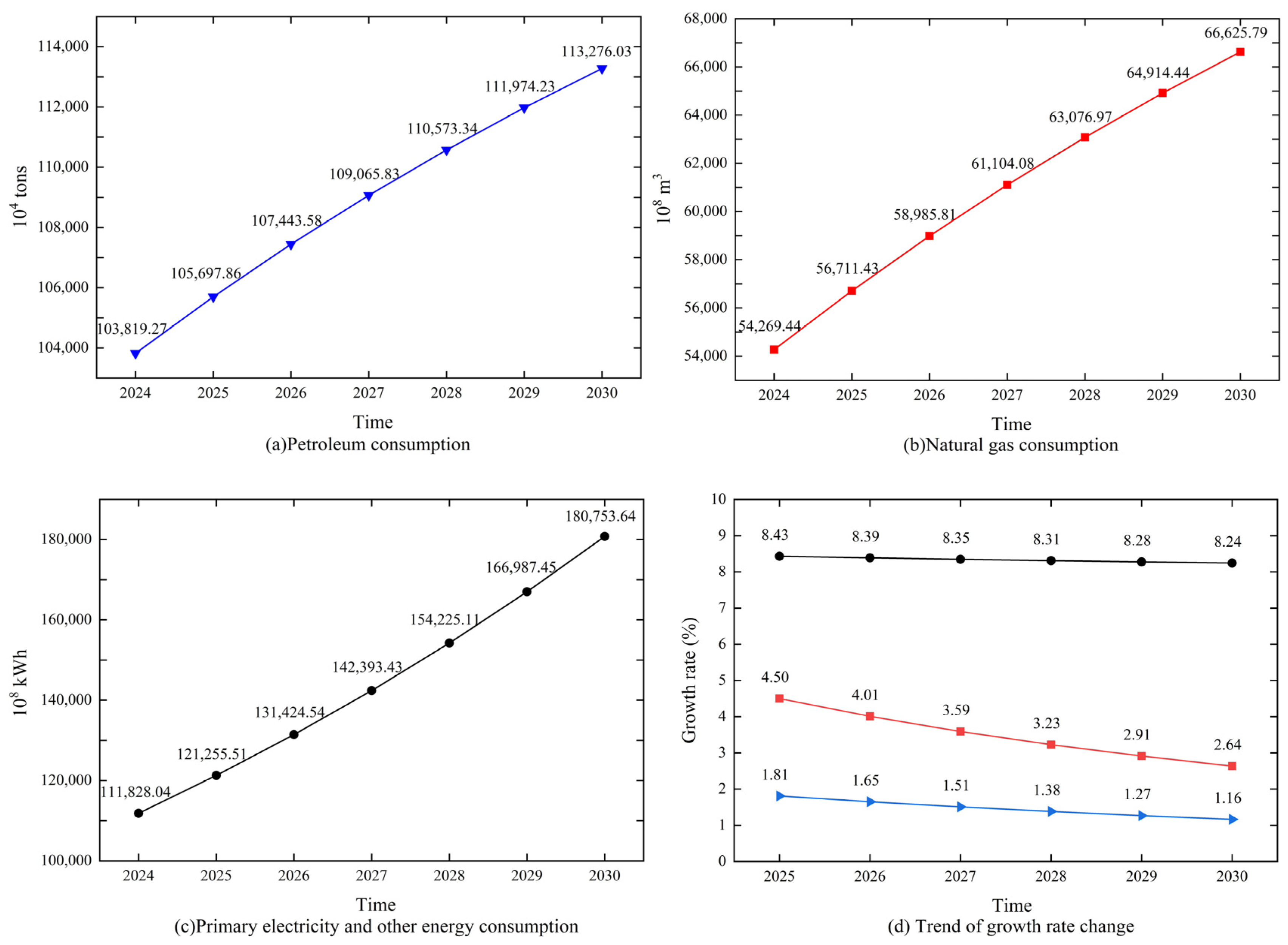
The predicted energy consumption data from this study are presented in

Table 5. Predicted energy consumption data (2024–2030).

Year	Petroleum	Natural Gas	Primary Electricity and Other Energy
2024	103,819.27	54,269.44	111,828.04
2025	105,697.86	56,711.43	121,255.51
2026	107,443.58	58,985.81	131,424.54
2027	109,065.83	61,104.08	142,393.43
2028	110,573.34	63,076.97	154,225.11
2029	111,974.23	64,914.44	166,987.45
2030	113,276.03	66,625.79	180,753.64

. Additionally, Figure 8 depicts the dynamic evolution of energy consumption data from 2024 to 2030.

Figure 8 illustrates the dynamic trend of the three energy types. As depicted in Figure 8a, from 2024 to 2030, annual petroleum consumption ranges between 1038.1927 and 1132.7603 million tons, exhibiting a gradual upward trend. Notably, the total petroleum consumption in 2030 increases by 94.5676 million tons compared with 2024. To measure the annual growth of petroleum consumption, this study calculates that its annual added values are 18.7859, 17.4572, 16.2225, 15.0751, 14.0088, and 13.0180 million tons, respectively. From this, we can see that between 2024 and 2030, the total oil consumption gradually increases, while the added value of its consumption decreases year by year.

As shown in Figure 8b, from 2024 to 2030, the natural gas usage ranges between 5426.944 and 6662.579 billion cubic meters and increases year by year. Specifically, natural gas consumption increases by 1235.635 billion cubic meters between 2024 and 2030. To further explore the annual added values of natural gas consumption, this research calculates that its annual added values are 244.199, 227.438, 211.827, 197.288, 183.747, and 171.135 billion cubic meters, respectively. Therefore, between 2024 and 2030, the total consumption of natural gas shows a gradually increasing trend, while the added value of its consumption shows a decreasing trend year by year.

Figure 8c demonstrates that the consumption of primary electricity and other energy sources also increases yearly within the forecast interval, with an annual consumption range of 11,182.804 to 18,075.364 billion kilowatt-hours. According to calculations, primary electricity and other energy consumption in 2030 increase by 6892.561 billion kilowatt-hours compared with 2024. To further explore its changes, this study calculates the added values of the annual consumption of primary electricity and other energy consumption over the seven years, which are 942.748, 1016.902, 1096.889, 1183.168, 1276.234, and 1376.619 billion kilowatt-hours, respectively. This analysis indicates that between 2024 and 2030, the total primary electricity and other energy consumption increases annually, with the added value of consumption rising each year.

To further analyze the future trends in annual growth rates, this study calculates the year-on-year growth rates for three types of energy consumption. It visualizes their trends, as illustrated in Figure 8d. According to Figure 8d, it is evident that the year-over-year increase of petroleum, natural gas, primary electricity and other energy consumption exhibits a monotonically decreasing trend. Notably, natural gas has the fastest decline rate, and petroleum has the second decline rate. In contrast, primary electricity and other energy sources have the gentlest decline trend, and their growth rate curves approximately show horizontal linear characteristics.

In conclusion, this research utilizes the TPBSVGM(1,1) to predict and analyze the dynamic trends in the consumption of the three energy sources from 2024 to 2030. The forecast findings reveal that during this period, the consumption of all three types of energy exhibits a growth trend. However, their growth rate shows varying degrees of decreasing characteristics. Therefore, based on the growth characteristics of various energy types, differentiated and practical management strategies should be formulated. On the one hand, it is necessary to reasonably control total energy consumption, curb the blind expansion of energy-intensive industries and reduce unreasonable energy consumption through energy efficiency improvements and refined management, thus ensuring a balance between energy supply and demand. On the other hand, it is necessary to guide key sectors such as industry and transportation to reduce their dependence on petroleum in high-energy-consuming links and strengthen policy support for natural gas, primary electricity and other energy sources, thereby promoting the green and low-carbon transformation of the energy structure and contributing to the achievement of national energy security and sustainable development goals.

In addition, TPBSVGM(1,1) has a relatively flexible structure and strong adaptability. It is not only applicable to energy consumption prediction in China but also has the potential to be further extended to other industries, such as industry, transportation, and construction, as well as countries and regions with different energy consumption patterns.

4. Conclusions

This study established TPBSVGM(1,1) utilizing the annual consumption data of petroleum, natural gas, primary electricity and other energy to conduct three sets of prediction experiments regarding energy consumption. To evaluate the prediction accuracy of TPBSVGM(1,1), this study compared it with GM(1,1) and FGM(1,1). By comparing the trends of predicted data of the three models with actual data and the error indices, this study validated the accuracy of TPBSVGM(1,1) in energy consumption prediction. Building upon these findings, this research employed the developed model for forecasting the consumption data of three energy types spanning 2024–2030, thereby analyzing the future dynamic changes and growth rate trends of energy consumption in China.

The main conclusions are as follows:

(1) This research introduced a novel three-parameter background value TPBSVGM(1,1) through tuning the parameters within the background values and utilizing the Simpson formula for reconstructing the background value. This proposed model was employed to predict energy consumption, thereby introducing a new method for forecasting energy consumption.

(2) This research verifies that the introduced TPBSVGM(1,1) exhibits superior accuracy in energy consumption prediction relative to the comparison models, as evidenced by the findings from Experiments 1 to 3. Furthermore, this study also confirms that the prediction precision of TPBSVGM(1,1) in energy consumption achieves an “excellent” level.

(3) This study utilized the proposed TPBSVGM(1,1) to forecast three types of energy consumption data spanning 2024–2030, thereby clarifying the dynamic evolution trends and growth rate situation. The research findings indicate that the three energy consumption categories exhibit different growth trends, and their growth rate shows varying degrees of decline characteristics.

However, this study has certain limitations: (1) This study employed the proposed grey univariate TPBSVGM(1,1) to forecast energy consumption without considering the impact of external elements. Future research can introduce influencing factors such as industrial structure and economic variables, and utilize a grey multivariate model to conduct prediction experiments. This approach would further enrich and enhance the models and methods for predicting energy consumption. (2) This research utilized the Simpson formula to reconstruct background values. However, in some cases, the variation pattern of the data may change over different time periods, and the background values calculated with fixed weights may not be able to adapt to these changes. Future studies could incorporate adaptive accumulation based on TPBSVGM(1,1) to more effectively capture data characteristics during different time intervals. This method can enhance the smoothness of background values and provide technical support for improving model prediction accuracy.

References

1. Zeng, S.; Su, B.; Zhang, M.; Gao, Y.; Liu, J.; Luo, S.; Tao, Q. Analysis and forecast of China’s energy consumption structure. Energy Policy 2021, 159, 112630. [Google Scholar] [CrossRef] [Scilit]
2. Gabr, E.M.; Mohamed, S.M. Energy management model to minimize fuel consumption and control harmful gas emissions. Int. J. Energy Water Res. 2020, 4, 453–463. [Google Scholar] [CrossRef] [Scilit]
3. Xu, G.; Schwarz, P.; Yang, H. Adjusting energy consumption structure to achieve China’s CO2 emissions peak. Renew. Sustain. Energy Rev. 2020, 122, 109737. [Google Scholar] [CrossRef] [Scilit]
4. Hwang, Q.; Yao, M.; Li, S.; Wang, F.; Luo, Z.; Li, Z.; Liu, T. Risk spillovers between China’s carbon and energy markets. Energies 2023, 16, 6820. [Google Scholar] [CrossRef] [Scilit]
5. Li, Y.; Chen, Y.; Cai, Q.; Zhu, L. Calculation of CO2 emissions from China at regional scales using remote sensing data. Remote Sens. 2024, 16, 544. [Google Scholar] [CrossRef] [Scilit]
6. Wang, S.; Wu, J.; Xiang, M.; Wang, S.; Xie, X.; Lv, L.; Huang, G. Multi-objective optimisation model of a low-cost path to peaking carbon dioxide emissions and carbon neutrality in China. Sci. Total Environ. 2024, 912, 169386. [Google Scholar] [CrossRef] [Scilit]
7. Adebayo, T.S.; Rjoub, H. A new perspective into the impact of renewable and nonrenewable energy consumption on environmental degradation in Argentina: A time–frequency analysis. Environ. Sci. Pollut. Res. Int. 2022, 29, 16028–16044. [Google Scholar] [CrossRef] [Scilit]
8. Zhang, D.; Wang, J.; Lin, Y.; Si, Y.; Huang, C.; Yang, J.; Huang, B.; Li, W. Present situation and future prospect of renewable energy in China. Renew. Sustain. Energy Rev. 2017, 76, 865–871. [Google Scholar] [CrossRef] [Scilit]
9. Xiao, H.; Ma, Z.; Zhang, P.; Liu, M. Study of the impact of energy consumption structure on carbon emission intensity in China from the perspective of spatial effects. Nat. Hazards 2019, 99, 1365–1380. [Google Scholar] [CrossRef] [Scilit]
10. Wang, Y.; Chen, J.; Cao, B.; Liu, X.; Zhang, X. Energy consumption prediction of cold storage based on LSTM with parameter optimization. Int. J. Refrig. 2025, 175, 12–24. [Google Scholar] [CrossRef] [Scilit]
11. Wu, S.; Wang, F.; Wan, M. Energy consumption prediction of new energy vehicles in smart city based on LSTM network. Int. J. Glob. Energy Issues 2022, 44, 484–497. [Google Scholar] [CrossRef] [Scilit]
12. Uzun, E.; Karabinaoğlu, M.S.; Ayaz, M. LSTM-based estimation of energy consumption in energy-intensive facilities. Eng. Res. Express 2025, 7, 015420. [Google Scholar] [CrossRef] [Scilit]
13. Hou, Y.; Wang, X.; Chang, H.; Dong, Y.; Zhang, D.; Wei, C.; Lee, I.; Yang, Y.; Liu, Y.; Zhang, J. Natural gas consumption monitoring based on k-NN algorithm and consumption prediction framework based on backpropagation neural network. Buildings 2024, 14, 627. [Google Scholar] [CrossRef] [Scilit]
14. Jia, A.; Cheng, G.; Chen, W.; Li, Y. Forecast of natural gas supply and demand in China under the background of “Dual Carbon Targets”. Petrol. Explor. Dev. 2023, 50, 492–504. [Google Scholar] [CrossRef] [Scilit]
15. Wang, C.; Zhu, M. Scenario prediction of China’s natural gas consumption and carbon emissions in the next ten years. Front. Econ. China 2021, 16, 569–587. [Google Scholar] [CrossRef] [Scilit]
16. Janjua, J.I.; Ahmad, R.; Abbas, S.; Mohammed, A.S.; Khan, M.S.; Daud, A.; Abbas, T.; Khan, M.A. Enhancing smart grid electricity prediction with the fusion of intelligent modeling and XAI integration. Int. J. Adv. Appl. Sci. 2024, 11, 230–248. [Google Scholar] [CrossRef] [Scilit]
17. Anh, L.H.; Yu, G.H.; Vu, D.T.; Kim, J.S.; Lee, J.I.; Yoon, J.C.; Kim, J.Y. Stride-TCN for energy consumption forecasting and its optimization. Appl. Sci. 2022, 12, 9422. [Google Scholar] [CrossRef] [Scilit]
18. Luo, C.; Liu, C.; Huang, C.; Qiu, M.; Li, D. Arima markov model and its application of China’s total energy consumption. Energies 2025, 18, 2914. [Google Scholar] [CrossRef] [Scilit]
19. Prakash, C.; Dhyani, B.; Chauhan, A.; Sayal, A. Arima based forecasting of solar and hydro energy consumption with implications for grid stability and renewable policy. Discov. Sustain. 2025, 6, 663. [Google Scholar] [CrossRef] [Scilit]
20. Zhang, Y.; Mao, S.; Kang, Y. A clean energy forecasting model based on artificial intelligence and fractional derivative grey Bernoulli models. Grey Syst. Theor. Appl. 2021, 11, 571–595. [Google Scholar] [CrossRef] [Scilit]
21. Olabi, A.G.; Haridy, S.; Sayed, E.T.; Radi, M.; Alami, A.; Zwayyed, F.; Salameh, T.; Abdelkareem, M. Implementation of artificial intelligence in modeling and control of heat pipes: A review. Energies 2023, 16, 760. [Google Scholar] [CrossRef] [Scilit]
22. Blackburn, M.L. Bias in small-sample inference with count-data models. Am. Stat. 2020, 74, 267–273. [Google Scholar] [CrossRef] [Scilit]
23. Çakır, S. Renewable energy generation forecasting in Turkey via intuitionistic fuzzy time series approach. Renew. Energy 2023, 214, 194–200. [Google Scholar] [CrossRef] [Scilit]
24. Zhicun, X.; Meng, D.; Lifeng, W. Evaluating the effect of sample length on forecasting validity of FGM(1,1). Alex. Eng. 2020, 59, 4687–4698. [Google Scholar] [CrossRef] [Scilit]
25. Wu, W.; Ma, X.; Zeng, B.; Zhang, Y.; Li, W. Forecasting short-term solar energy generation in Asia Pacific using a nonlinear grey Bernoulli model with time power term. Energy Environ. 2021, 32, 759–783. [Google Scholar] [CrossRef] [Scilit]
26. Yuan, W.; Rui, Z.; Bao, Y.; Xiang, H.; Bo, L. Grain yield prediction based on the improved unbiased grey markov model. Discrete Dyn. Nat. Soc. 2025, 2025, 8282138. [Google Scholar] [CrossRef] [Scilit]
27. Li, S.; Zeng, B.; Ma, X.; Zhang, D. A novel grey model with A three-parameter background value and its application in forecasting average annual water consumption per capita in urban areas along the Yangtze River basin. Grey Syst. 2020, 32, 118–132. [Google Scholar]
28. Liu, C.; Lao, T.; Wu, W.Z.; Xie, W. Application of optimized fractional grey model-based variable background value to predict electricity consumption. Fractals 2021, 29, 2150038. [Google Scholar] [CrossRef] [Scilit]
29. Zhang, S.; An, H.K.; Yin, H. Intelligent trapezoid and variable weight combination-based reconstructed GM model. Heliyon 2024, 10, e35889. [Google Scholar] [CrossRef] [Scilit]
30. Cao, X.D.; Shi, Q.; Chen, Y.K.; Chen, C.C. Short-term traffic flow uncertainty prediction based on novel GM(1,1). Promet-Traffic Transp. 2024, 36, 450–462. [Google Scholar] [CrossRef] [Scilit]
31. Huang, H.; Tao, Z.; Liu, J.; Cheng, J.; Chen, H. Exploiting fractional accumulation and background value optimization in multivariate interval grey prediction model and its application. Eng. Appl. Artif. Intell. 2021, 104, 104360. [Google Scholar] [CrossRef] [Scilit]
32. Wang, H.; Li, Y. A novel seasonal grey prediction model with fractional order accumulation for energy forecasting. Heliyon 2024, 10, e29960. [Google Scholar] [CrossRef] [Scilit] [PubMed]
33. Li, S.; Gong, K.; Song, N.; Zeng, B. Forecasting China’s natural gas external dependence under the “Dual Carbon” goals by a new grey model. Sci. Prog. 2023, 106, 368504231157707. [Google Scholar] [CrossRef] [Scilit] [PubMed]
34. Sun, J.; Li, H.; Zeng, B.; Zhao, X.; Wang, C. Parameter optimization on the three-parameter whitenization grey model and its application in simulation and prediction of gross enrollment rate of higher education in China. Complexity 2020, 2020, 6640000. [Google Scholar] [CrossRef] [Scilit]
35. Zhu, J.N.; Liu, X.C.; Liu, C. Non-equidistant non-homogenous grey prediction model with fractional accumulation and its application. Intell. Fuzzy Syst. 2021, 40, 11861–11874. [Google Scholar] [CrossRef] [Scilit]
36. Xu, X.; Wu, Y.; Zeng, B. Forecasting short-term energy consumption in Chongqing using a novel grey Bernoulli model. Grey Syst. Theor. Appl. 2025, 15, 21–44. [Google Scholar] [CrossRef] [Scilit]
37. Zhou, W.; Zeng, B.; Wu, Y.; Wang, J.; Li, H.; Zhang, Z. Application of the three-parameter discrete direct grey model to forecast China’s natural gas consumption. Soft Comput. 2023, 27, 3213–3228. [Google Scholar] [CrossRef] [Scilit]
38. Ren, L.; Gao, Y.; Yang, F.; He, Y. Predicting solar array power output on a spacecraft using a fractional-order grey model and particle swarm optimization. Grey Syst. 2024, 36, 86–97. [Google Scholar]
39. Wu, W.; Ma, X.; Wang, Y.; Cai, W.; Zeng, B. Predicting primary energy consumption using NDGM(1,1,k,c) model with Simpson formula. Sci. Iran. 2021, 28, 3379–3395. [Google Scholar]
40. Ma, X.; Wu, W.; Zhang, Y. Improved GM(1,1) model based on Simpson formula and its applications. Grey Syst. 2019, 31, 33–46. [Google Scholar]
41. Li, X.; Yang, J.; Zhao, Y.; Zhou, S.; Wu, Y. Prediction and assessment of marine fisheries carbon sink in China based on a novel nonlinear grey Bernoulli model with multiple optimizations. Sci. Total Environ. 2024, 914, 169769. [Google Scholar] [CrossRef] [Scilit]
42. Li, H.; Ma, Y.; Zhu, H. Forecasting the evolution of public opinion using a novel improved grey model during emergencies. Grey Syst. 2023, 35, 87–104. [Google Scholar]
43. Ding, S.; Li, R. Forecasting the sales and stock of electric vehicles using a novel self-adaptive optimized grey model. Eng. Appl. Artif. Intell. 2021, 100, 104148. [Google Scholar] [CrossRef] [Scilit]
44. Wang, M.; Wang, W.; Wu, L. Application of a new grey multivariate forecasting model in the forecasting of energy consumption in 7 regions of China. Energy 2022, 243, 123024. [Google Scholar] [CrossRef] [Scilit]
Figure 1. Flow diagram of TPBSVGM(1,1).
Applsci 16 02855 g001
Figure 2. Change trends between true and forecasted values in Experiment 1.
Applsci 16 02855 g002
Figure 3. Comparison of error indicators for Experiment 1.
Applsci 16 02855 g003
Figure 4. Change trends between true and forecasted values in Experiment 2.
Applsci 16 02855 g004
Figure 5. Comparison of error indicators for Experiment 2.
Applsci 16 02855 g005
Figure 6. Change trends between true and forecasted values in Experiment 3.
Applsci 16 02855 g006
Figure 7. Comparison of error indicators for Experiment 3.
Applsci 16 02855 g007
Figure 8. Predicted energy consumption trends (2024–2030).
Applsci 16 02855 g008