Operational Optimisation of the Medium-Voltage Network Containing Renewable Energy Sources and Energy Storage

Abstract

The rapid growth of renewable electricity generation introduces technical challenges that were previously uncommon. These include, for example, problems with exceeding the permissible voltage values in network nodes, overloading of transformers and line sections located behind the transformer, as well as balance problems. This article proposes an original methodology for eliminating these problems. Four objective functions reflecting different operator priorities were used. Attention is drawn to the increasing importance of the development of electricity storage. The results confirm that coordinated optimisation of voltage regulation, energy storage, and flexible load management enables increased renewable energy connection capacity while reducing power losses and improving the grid voltage profile. The case study results demonstrate the effectiveness of the proposed approach under the considered operating scenarios. The proposed tool can support network operators in managing MV grid operation under the considered scenarios. The ongoing energy transition requires network operators to react quickly to emerging problems. Therefore, advanced computational methods are needed to mitigate operational risks and respond to emerging constraints.

1. Introduction

Modern power grids face many challenges related to the dynamic development of renewable energy sources (RESs). One of the key elements of this process is the integration of photovoltaic (PV) and wind farms (WFs) with medium-voltage (MV) networks, which requires their optimisation in terms of stability and energy efficiency [1]. Unlike conventional energy sources, such as coal or gas power plants, RESs are characterised by significant variability in generation depending on weather conditions. Fluctuations in solar radiation and wind speed lead to irregular changes in voltage and power flows, which can negatively affect the operation of the power grid [2]. One of the main problems resulting from the growing share of distributed generation in MV networks is the increase in voltage levels, especially during peak hours of energy production from RESs [3]. This increase can cause voltages to exceed permissible limits, leading to undesirable effects in distribution networks [4]. In addition, voltage fluctuations can negatively affect the quality of electricity, causing unstable operation of loads and inverter tripping in PV plants, and potentially propagating to low-voltage distribution networks [1]. Another important issue is an increase in active power losses in the medium-voltage network. Fluctuations in power generated by RESs lead to inefficient energy distribution and increased reactive power flows, which in turn results in greater losses in transmission lines and transformers [5]. In extreme cases, this can lead to deterioration in the efficiency of the entire power system and an increase in operating costs. Optimisation of the operation of the medium-voltage network in the context of the growing penetration of renewable sources is therefore a necessary step towards increasing the reliability, efficiency and stability of the power system. This paper selected methods of improving the operating conditions of MV networks, allowing for more effective use of the potential of RESs while minimising the negative effects of their operation.

The main contributions are:

• Four objective-function formulations reflecting different operator priorities (power losses/voltage quality/cost/hosting capacity).
• Coordinated optimisation of OLTC, PV inverter reactive power, storage placement/dispatch, and IPC/DSM within one framework.
• A MATLAB (R2025b) and PowerFactory (PowerFactory 2024) co-simulation workflow and a comparative evaluation of 15 metaheuristics in the same MV case study.

2. Literature Review

One of the optimisation tasks in medium-voltage networks is the appropriate location and proper selection of installed energy storage capacity. Energy storage can effectively compensate for fluctuations in RES generation by accumulating surplus energy during peak production periods and returning it to the network during periods of low generation or increased demand. An optimal layout allows for local power balancing, which minimises line overloads and reduces the need to transmit energy over long distances, thus reducing active power losses [6]. Additionally, appropriately selected storage capacity allows for more effective regulation and equalisation of the voltage profile and increased flexibility of the MV network [7]. The article discusses the criteria for selecting the optimal location and technical parameters of energy storage, which can significantly improve the stability and efficiency of the power system in the context of the growing share of renewable sources. Another mechanism for improving the operating conditions of the medium-voltage network in the face of the growing share of photovoltaic and wind farms is voltage regulation by controlling the flow of reactive power [8]. Inverters used in RES installations can operate in a constant power factor (cosφ) mode or in various control methods by adjusting the level of generated or consumed reactive power. Thanks to an appropriate control algorithm, they can limit voltage increases in the network during peak hours of generation and reduce voltage drops during periods of lower energy production [9,10]. An additional advantage of active reactive power management is the reduction in active power losses in lines and transformers. Reducing excessive reactive power flows allows for better use of the transmission capacity of the network, increasing its operational efficiency. In addition, appropriate control of inverters in the dynamic reactive power compensation mode can reduce the demand for conventional compensation devices, such as capacitor banks or chokes, thus reducing the investment and operating costs of the network. One of the effective ways to reduce balance problems, and thus also potential voltage deviations in networks, and reduce active power losses is to use the service of interventional increase in active power consumption (IPC) by industrial plants. This mechanism consists of adjusting selected industrial loads in response to system-balance conditions in response to system-balance problems, which may also affect voltage changes in the network, especially during peak hours of energy generation from RESs. In practice, this solution can be implemented through demand management systems (Demand Side Management—DSM), which enable flexible control of the operation of selected industrial receivers [11,12]. In the event of excessive power generation in the power system, industrial plants can increase periodic energy consumption, for example by starting selected additional energy-intensive production processes [13]. Such actions locally increase active power consumption, which leads to a reduction in the surplus energy introduced to the network by RESs and, consequently, changes in voltage levels. An additional benefit of this mechanism is the reduction in active power losses in lines and transformers [1]. Consuming electricity closer to its source reduces the need for transmission, which results in a reduction in currents flowing in the network and thus a reduction in transmission losses.

In the process of planning the development of the power grid and connecting subsequent renewable energy sources, an important technical issue that requires a detailed analysis of the power system operating parameters is the determination of the maximum power that can be connected, referred to as the “hosting capacity”. The key limitations result primarily from the voltage value, transmission capacity of lines and transformers, as well as the need to balance power in the system [14]. To precisely determine the limit value of power that can be safely connected to the grid, various analytical and simulation methods are used [15,16,17]. The analysis of power flows allows for the assessment of the network’s ability to absorb additional generation and the identification of states in which the permissible parameters are exceeded. In turn, mathematical optimisation methods based on metaheuristic algorithms [18] allow for the determination of the value of the connected power considering all the required network constraints [19]. Simulations enable the assessment of the variability of energy production from RESs and the variability of customer demand, which gives a more precise picture of the actual “network capacity”. A probabilistic approach is also often used in analyses that considers the uncertainty resulting from the irregular generation of renewable energy and fluctuations in power demand. Increasing attention is also being paid to the use of artificial intelligence and neural networks [20] in this regard. In many cases, it is also necessary to modernise the MV network, including replacing transformers with on-load tap regulation [21], increasing the cross-sections of conductors and using modern network automation systems that allow for more effective management of energy flows.

In recent years, it has been increasingly emphasised that the use of a single flexibility mechanism is not sufficient to ensure the safe and efficient operation of medium-voltage networks with a high share of renewable energy sources [14]. Increasing attention is being paid to the need for coordinated optimisation of multiple flexibility sources, allowing for fuller utilisation of the grid’s potential while maintaining its technical limitations [15].

Most of the work done to date has used single-objective functions. An additional limitation is the use of sequential approaches, in which planning decisions (e.g., the location of energy storage facilities or new PV sources) are made independently of subsequent operational optimisation [17,22]. This leads to the omission of important relationships between long-term decisions and short-term control.

The literature offers a wide range of metaheuristic algorithms used to solve optimisation problems in the power industry [19]. The results obtained with these algorithms may vary. There is therefore a need to compare the performance of different optimisation algorithms in order to ensure the reliability of the results obtained [23].

3. Description of the Research Methodology

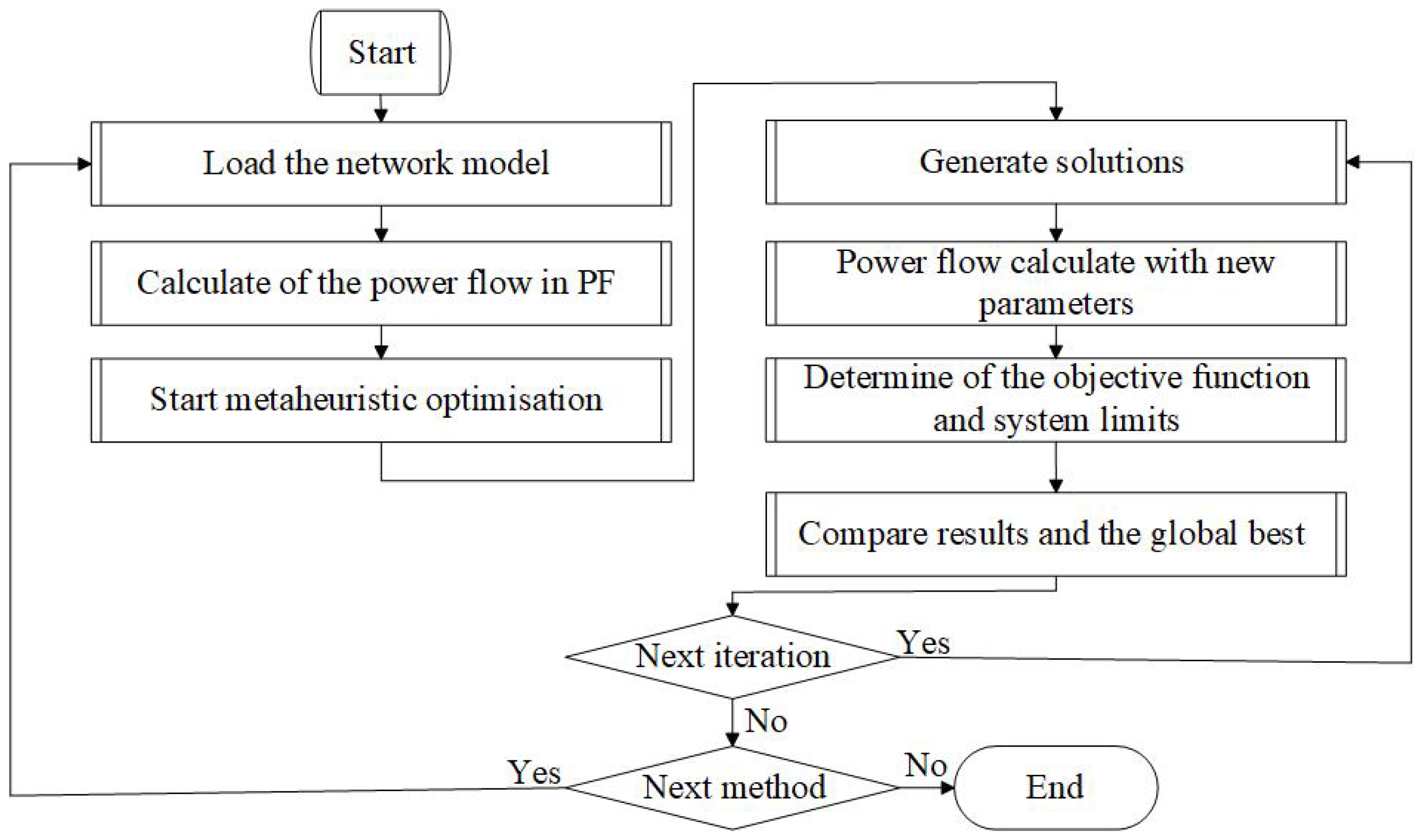
The research problem under consideration concerns determining the optimal operating conditions of the MV network from the point of view of the considered objective functions. The values of the decision variable vectors obtained as a result of optimisation indicate the state in which the objective function composed of one or more indicators has reached the minimum value. 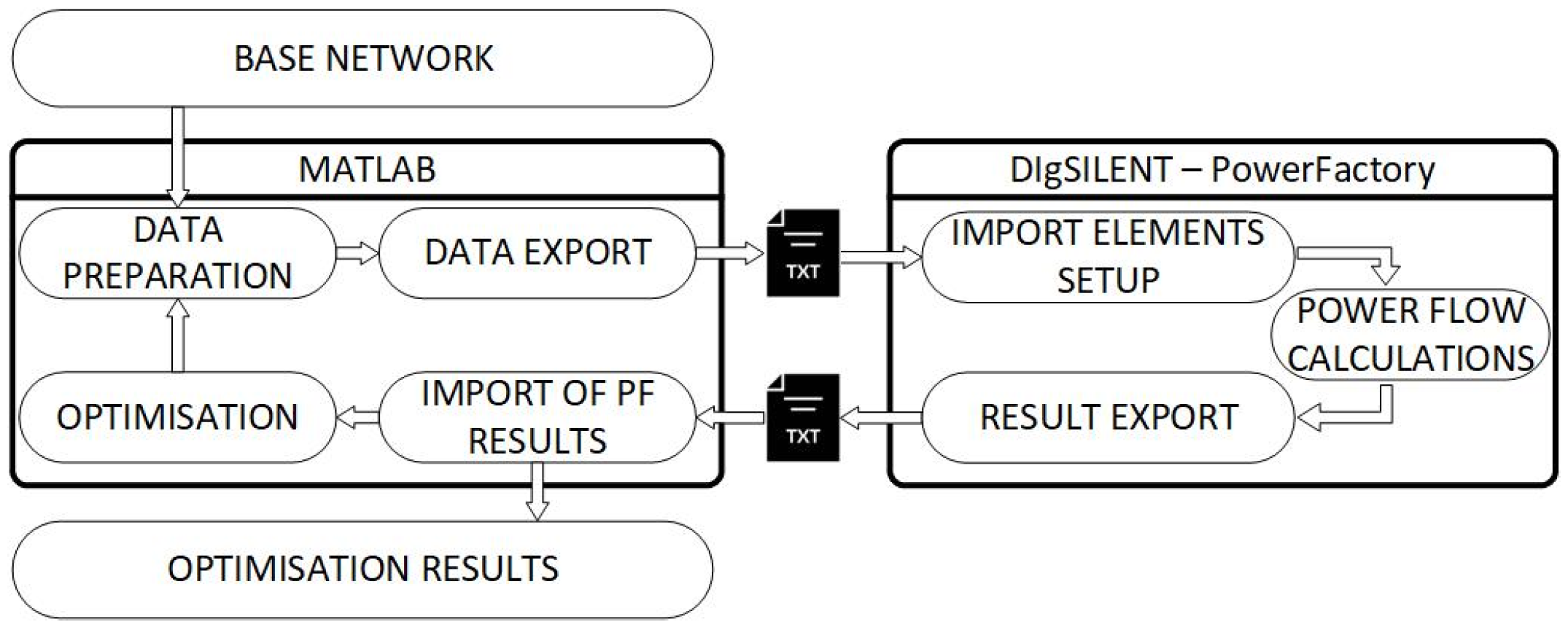The general algorithm of the proposed calculation methodology is presented in Figure 1. The main program script was written in MATLAB, and the power flow calculations were performed in PowerFactory (PF). Both programs, during the calculation process in subsequent iterations, exchanged data (according to Figure 2). By combining two advanced tools (MATLAB and PowerFactory), we developed a co-simulation workflow for the considered optimisation tasks.

Figure 1 summarises the overall workflow of the proposed MATLAB–PowerFactory co-simulation. In Stage 1, the optimisation is performed sequentially using F_obj1–F_obj4, each reflecting a different operator priority. Stage 2 then performs a final refinement of operating set-points for the best feasible configuration obtained after Stage 1.

The optimisation process is repeated in a loop until the stopping criterion corresponding to the execution of a given number of iterations is met. All metaheuristic algorithms were executed under the same computational budget. Each run used 1000 iterations, and the population size was set equal to the number of decision variables. Moreover, all methods were constrained to the same number of PowerFactory power-flow evaluations, ensuring an equal number of objective-function calls across algorithms.

The optimisation considers the following control variables:

• The OLTC tap position of the HV/MV transformer, selected discretely in the range from −8 to +8. The tap is adjusted to keep the MV-side voltage as close as possible to the target value of 1.05 p.u.;
• Active and reactive power set-points of PV inverters. The PV active power is optimised, while the reactive power follows a power-factor-based control with tanφ in range −0.4 to 0.4;
• Two energy storage units (ESs) are optimised simultaneously: in each candidate solution, the locations of both ES units are selected from all load buses, and their active/reactive power set-points are optimised;
• Interventional power consumption increase (IPC), implemented as a DSM service, is modelled as an additional controllable load bounded only by its admissible power range.

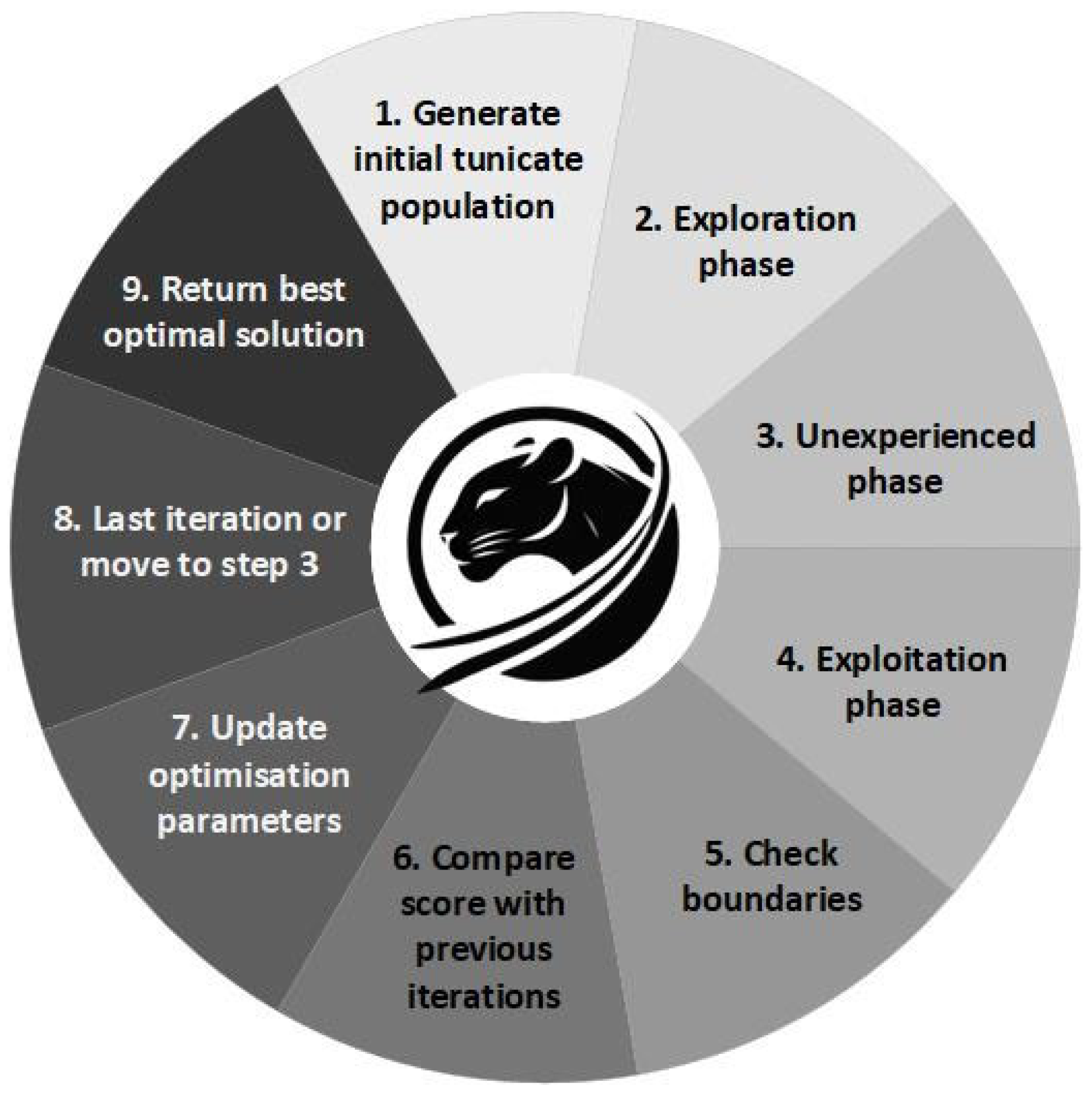
Metaheuristic optimisation methods, often inspired by animal behaviour, are an effective tool in solving complex optimisation problems in power systems. They are based on modelling natural adaptation mechanisms and resource search strategies used by various animal species, such as insect swarms, bird flocks or fish schools. These algorithms use the ability of the population to explore and exploit the solution space in a dynamic and adaptive manner, allowing them to search for high-quality (near-optimal) solutions without exhaustive exploration of the full search space. Due to their flexibility and computational efficiency, they are widely used in solving various optimisation tasks in power engineering, including problems related to voltage regulation, minimising power losses and optimal deployment of renewable sources and energy storage. An example optimisation run based on the PO method [24] is presented in Figure 3.

The study used classical and well-known metaheuristic methods such as Particle Swarm Optimisation (PSO) [25], Cuckoo Search (CUC) [26], Grey Wolf Optimiser (GWO) [27], Moth–Flame Optimisation (MFO) [28], Whale Optimisation Algorithm (WOA) [29], Fox Optimisation Algorithm (FOX) [30] and Wild Horse Optimisation (WHO) [31]. They also included new methods that have only recently started to be used: Puma Optimiser (PO) [24], Elk Herd Optimiser (EHO) [32], Greylag Goose Optimisation (GGO) [33], Walrus Optimiser (WO) [34], Secretary Bird Optimisation Algorithm (SBOA) [35] and Arctic Puffin Optimisation (APO) [36]. Each of these algorithms draws inspiration from unique adaptation strategies of animals to their natural environment. In addition to metaheuristic methods inspired by animal behaviour, algorithms based on classical mathematical methods, such as Gradient-Based Optimiser (GBO) [37] and Newton–Raphson-Based Optimiser (NRO) [38], have also been used in power system optimisation research. The inspiration and year of invention of each method are summarised in

Table 1. Comparison of information on the metaheuristic methods used.

Method	Year	Inspiration
PSO [25]	1995	Group of animals
MFO [28]	2015	Moth
WOA [29]	2016	Whales
FOX [30]	2023	Fox
GGO [33]	2024	Greylag goose
WO [34]	2024	Walrus
PO [24]	2024	Puma
GBO [37]	2020	Gradient method
NRO [38]	2024	Newton–Raphson method
GWO [27]	2014	Grey wolf
APO [36]	2024	Arctic puffins
CUC [26]	2009	Cuckoos
WHO [31]	2022	Wild horses
SBOA [35]	2024	Secretary bird
EHO [32]	2024	Elk herd

.

In the optimisation studies, the key element was the minimisation of appropriately selected original objective functions, which consider important parameters related to the operation of the medium-voltage power grid. In the optimisation process, weighting factors were used, which allow for the unification of the levels of the size of various function components and their impact on the final optimisation result. For each objective function, the weights w_n were selected to bring the individual components to a comparable numerical scale. This normalisation was necessary due to large differences in orders of magnitude between terms (e.g., voltage-quality indices [39], losses, and cost terms), which otherwise would prevent meaningful comparison and aggregation. Depending on the objective definition, three or four components are used; in each case, the corresponding weights sum to 1.

$$F_{\mathrm{obj}\_1}\left(x\right)=w_1\cdot d{P}_{l\mathrm{oss}}+w_2\cdot U_{\mathrm{dev}}+w_3\cdot E_{\mathrm{opt}}$$

(1)

dP_loss—relative power losses; U_dev—coefficient of the standard deviation of the voltage in nodes; E_opt—coefficient of the costs of installing storage facilities.

$$d{P}_{\mathrm{loss}}={\displaystyle \frac{\Delta P}{P_{\mathrm{ld}}}}$$

(2)

ΔP—total power losses in the network; P_ld—total power drawn from the network.

$$U_{\mathrm{dev}}=\sqrt{{\displaystyle \frac{1}{N}}\cdot {{\displaystyle \sum _{i=1}^N\left(\frac{U_{\mathrm{i}}-U_0}{U_0}\right)}}^2}$$

(3)

N—number of nodes in the network; U_i—voltage value in the node; U₀—target voltage value in the node (1.05 U_n)

$$E_{\mathrm{opt}}={\displaystyle \frac{C_i}{C_{\max }}}\cdot {\displaystyle \sum \frac{E_c}{E_{\max }}}$$

(4)

C_i—cost of the energy storage per MWh of capacity; C_max—cost of the energy storage for the maximum installed capacity; E_c—total energy of the storage; E_max—total maximum energy of the storage,

A constant unit cost per MWh of storage energy capacity was assumed. The required energy capacity was linked to the rated power by assuming a fixed discharge duration of 4 h. This assumption reflects typical real-world BESS installations and operational needs in MV networks.

$$E_{\mathrm{c}}={\displaystyle \sum P_{\mathrm{ES}}}\cdot T$$

(5)

P_ES—power of energy storage

$$E_{\max }=P_{\mathrm{ES}\_\max }\cdot T$$

(6)

P_{ES_max}—total maximum power of storage facilities; T—required operating time of energy storage facilities [h]

$$C_{\max }=C_i\cdot E_{\max }$$

(7)

$$F_{\mathrm{obj}\_2}\left(x\right)=w_1\cdot d{P}_{\mathrm{loss}}+w_2\cdot U_{\mathrm{dev}}+w_3\cdot E_{\mathrm{opt}}+w_4\cdot P_{\mathrm{PV}\_\mathrm{cap}}$$

(8)

P_{PV_cap}—relative network capacity factor.

$$P_{\mathrm{PV}\_\mathrm{cap}}=1-\left({\displaystyle \sum P_{\mathrm{PV}}}/{\displaystyle \sum P_{\mathrm{PV}\_\max }}\right)$$

(9)

P_PV—installed capacity of PV installations; P_{PV_max}—total maximum power of PV installations.

$$F_{\mathrm{obj}\_3}\left(x\right)=P_{\mathrm{PV}\_\mathrm{cap}}$$

(10)

Selecting the appropriate objective function in the optimisation process allows for adjusting the network development strategy to the priorities of the power system operator. The first function is used in cases where the main goal is to improve the voltage profile and minimise active power losses and the costs of purchasing energy storage. The second objective function, in addition to the components that are in the first objective function, contains a component that allows for maximising the share of RESs, which is particularly important in the context of energy transformation. The third function allows for determining the maximum network capacity for RESs, which is the basis for future investment decisions regarding the modernisation of the power infrastructure [22].

$$F_{\mathrm{obj}\_4}\left(x\right)=w_1\cdot d{P}_{\mathrm{loss}}+w_2\cdot U_{\mathrm{dev}}$$

(11)

As noted earlier, in the calculations for objective functions F_obj1, F_obj2, and F_obj4, the weight values were selected so that the individual components of the objective function would take on similar values. In line with the expectations of network operators, the individual objectives were assumed to be equal. The article emphasises the possibility of reflecting the results in practice.

In Stage 1, the optimisation is carried out using a sequence of objective functions. First, the search is directed towards improving the operating performance of the network by prioritising voltage quality, losses, and storage-related cost (F_obj1). Next, the same criteria are considered while additionally promoting higher PV utilisation (F_obj2). Subsequently, the procedure focuses on maximising the feasible PV hosting level (maximum admissible PV penetration) under the adopted operating state and constraints (F_obj3). Finally, the best feasible solution is used as the base configuration. In Stage 2, this configuration is kept fixed, and a final refinement (re-optimisation) is performed only for the remaining continuous control variables (e.g., inverter reactive power set-points, OLTC tap position, and/or IPC/DSM level within bounds) to further reduce constraint violations and improve the objective value without changing the selected planning decisions.

During the optimisation, candidate solutions that violate operational limits are penalised. The penalty is applied when the loading of any MV line or the HV/MV transformer exceeds 100% of its rated power. Additionally, the penalty is applied when the voltage magnitude at any bus is outside the admissible range of 0.9–1.1 p.u. The penalty increases with the magnitude of the violation, which discourages infeasible operating points and drives the search towards solutions satisfying grid-code constraints. If the power-flow calculation does not converge for a candidate solution, the solution is treated as infeasible and assigned a large penalty value so that it cannot be selected as optimal.

$$F_{\mathrm{obj}}^{\mathrm{penalized}}(x)=F_{\mathrm{obj}}(x)+F_{\mathrm{P}}(x)$$

(12)

$F_{\mathrm{obj}}(x)$—original objective function; $F_{\mathrm{obj}}^{\mathrm{penalized}}(x)$—new objective function with added penalty; $F_{\mathrm{P}}(x)$—penalty function.

Equality constraints [23]

$$P_{Gi}-P_{Di}-{\displaystyle \left|U_i\right|\sum _{j=1}^{NB}\left|U_j\right|}\left[G_{ij}\cdot \cos {\alpha }_{ij}+B_{ij}\cdot \sin {\alpha }_{ij}\right]=0$$

(13)

$$Q_{Gi}-Q_{Di}-\left|U_i\right|{\displaystyle \sum _{j=1}^{NB}\left|U_j\right|}\left[G_{ij}\cdot \cos {\alpha }_{ij}-B_{ij}\cdot \sin {\alpha }_{ij}\right]=0$$

(14)

P_Gi, Q_Gi—power generated in nodes; P_Di, Q_Di—power received in nodes; G_ij, B_ij—conductance and susceptance; NB—number of nodes; α_ij—denotes the voltage angle difference between buses i and j.

Inequality constraints

$$T_i^{\min }\le T_i\le T_i^{\max }$$

(15)

T_i—transformer tap position; T_i^min, T_i^max —lower and upper limits of transformer tap position

$$U_i^{\min }\le U_i\le U_i^{\max }$$

(16)

U_i—node voltage; U_i^min, U_i^max—permissible voltage limits

$$I_j\le I_j^{\max }$$

(17)

I_j—line current; I_J^max—permissible current value

$$P_{Si}^{\min }\le P_{Si}\le P_{Si}^{\max }$$

(18)

$$U_{Si}^{\min }\le U_{Si}\le U_{Si}^{\max }$$

(19)

P_Si, U_Si—active power and source voltage; P_Si^min, P_Si^max, U_Si^min, U_Si^max—lower and upper limits of source operating parameters

$$-0.4\cdot P_{\mathrm{PV},k}\le Q_{\mathrm{PV},k}\le 0.4\cdot P_{\mathrm{PV},k}$$

(20)

$$-P_{\mathrm{ESmax}}\le P_{\mathrm{ES},k}\le P_{\mathrm{ESmax}},P_{\mathrm{ESmax}}=5 \mathrm{MW}$$

(21)

$$0\le P_{\mathrm{LD}15}\le 2 \mathrm{MW}$$

(22)

$$0\le P_{\mathrm{LD}60}\le 1 \mathrm{MW}$$

(23)

P_PV,k—active power of the PV source in node k; P_ESmax—maximum storage power rating considered; P_LD15, P_LD60—maximum IPC power

The reactive power capability is defined as a function of the instantaneous active power output. Without such coupling, the inverter could operate as a pure reactive power compensator at nearly zero active power, which is not representative of typical PV inverter operation and would distort the hosting-capacity assessment. To improve readability, the following sections present the optimisation results progressively, starting from storage placement under basic operating conditions, followed by the inclusion of IPC, RES expansion, hosting-capacity maximisation, and final operational tuning.

4. Test Network Description

In the study, optimisation analyses were performed using a modified version of the IEEE 69 test network [40] (Figure 4), adapted to the conditions of the Polish medium-voltage power grid. The standard IEEE 69 test network is commonly used in studies on the management of MV distribution networks, integration of renewable energy sources (RESs) and strategies for their operation optimisation. This model reflects the actual structures of distribution networks, allowing the analysis of the impact of different control strategies and infrastructure expansion on its stable operation. The introduced changes concern voltage levels, line lengths and cross-sections, the selected HV/MV transformer equipped with an OLTC, as well as the distribution of loads and RESs. PV plants are located at buses 9, 15, 27, 35, 46, 50, 52, and 60, with a total installed capacity of 12.5 MW, while IPC loads are placed at buses 15 and 60. The adopted operating state (load and PV generation levels) is the base scenario used in all objective-function evaluations.

The adapted IEEE 69 network is a representation of the operating conditions of the actual medium-voltage network, enabling analyses of the impact of various energy management strategies and optimisation methods on its correct operation. Thanks to the use of this model, it was possible to verify the effectiveness of metaheuristic methods in the process of optimising network parameters, locating energy storage facilities and maximising the integration of renewable sources while maintaining safe operating conditions. Candidate ES locations include all load buses (excluding the slack bus); exactly two ES units are placed in each run.

5. Calculation Results and Discussion

To comprehensively assess the impact of the applied optimisation methods on the operation of the power grid, a series of calculations were carried out for four different objective functions. Each of them considered different optimisation priorities, which allowed for a multi-aspect analysis of the efficiency of the network operation after connecting new elements. The results of the research conducted provide information on the efficiency of the applied optimisation strategies, the impact of individual factors on the optimal operation and efficiency of the network, and the possibilities for further integration of renewable energy sources. The following paragraphs present detailed analyses of the results obtained for each of the described objective functions.

5.1. Selection of Location and Power of Energy Storage Facilities

In this section, calculations were performed to determine the location and capacity of two energy storage facilities connected to the medium-voltage line. Such storage facilities are currently planned to be connected by network operators. These storage facilities do not belong to consumers but to the network operator, who wants to increase the flexibility of the medium-voltage network and eliminate the main problems resulting from the operation of a large number of RESs.

Table 2. Results for F_obj1 without IPC.

Method	Time	Fobj	ES1	ES2	PES1	PES2
	h	-	Bus nr.	Bus nr.	MW	MW
PSO	01:16:50	0.44014491	27	46	3.31	0.21
MFO	01:12:36	0.44013857	27	46	3.33	0.20
WOA	01:19:52	0.44477943	27	46	3.70	0.35
FOX	01:16:18	0.45925217	16	8	4.45	0
GGO	01:21:21	0.44554871	25	43	3.75	0.25
WO	01:21:40	0.44016604	27	46	3.31	0.21
PO	01:20:18	0.44012079	27	46	3.34	0.20
GBO	01:22:39	0.45064204	27	15	1.91	2.68
NRO	01:23:23	0.44118711	27	45	3.37	0.30
GWO	01:21:07	0.44020236	27	46	3.30	0.21
APO	04:15:11	0.44050419	27	45	3.37	0.22
CUC	02:19:25	0.44016340	27	46	3.31	0.21
WHO	02:28:34	0.44012303	27	46	3.32	0.20
SBOA	02:22:30	0.44015781	27	46	3.30	0.21
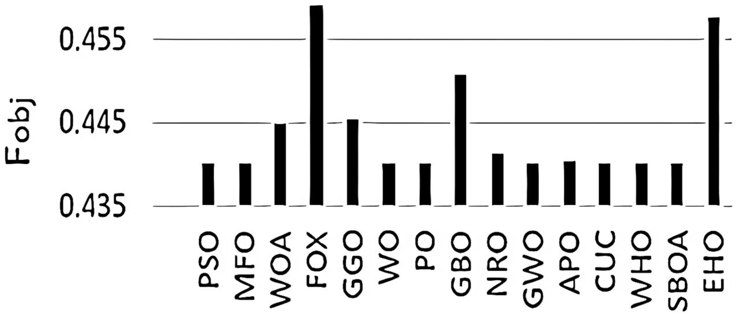
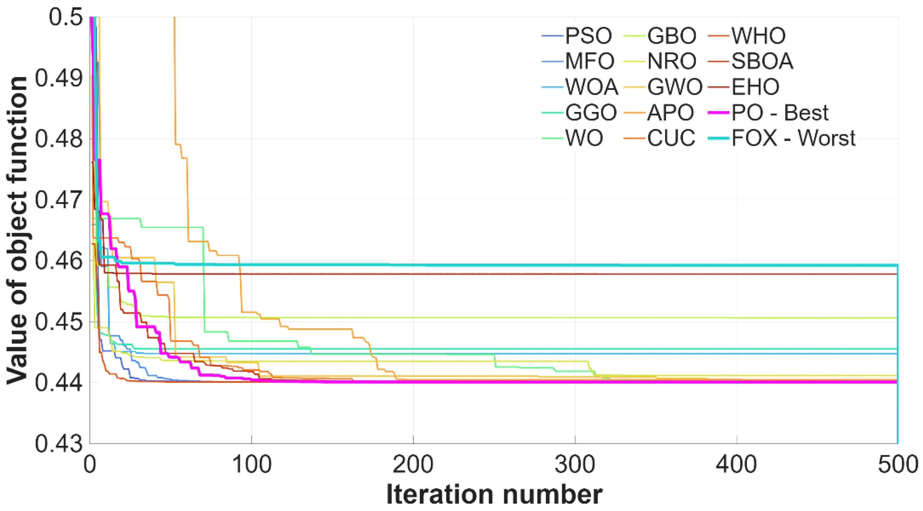
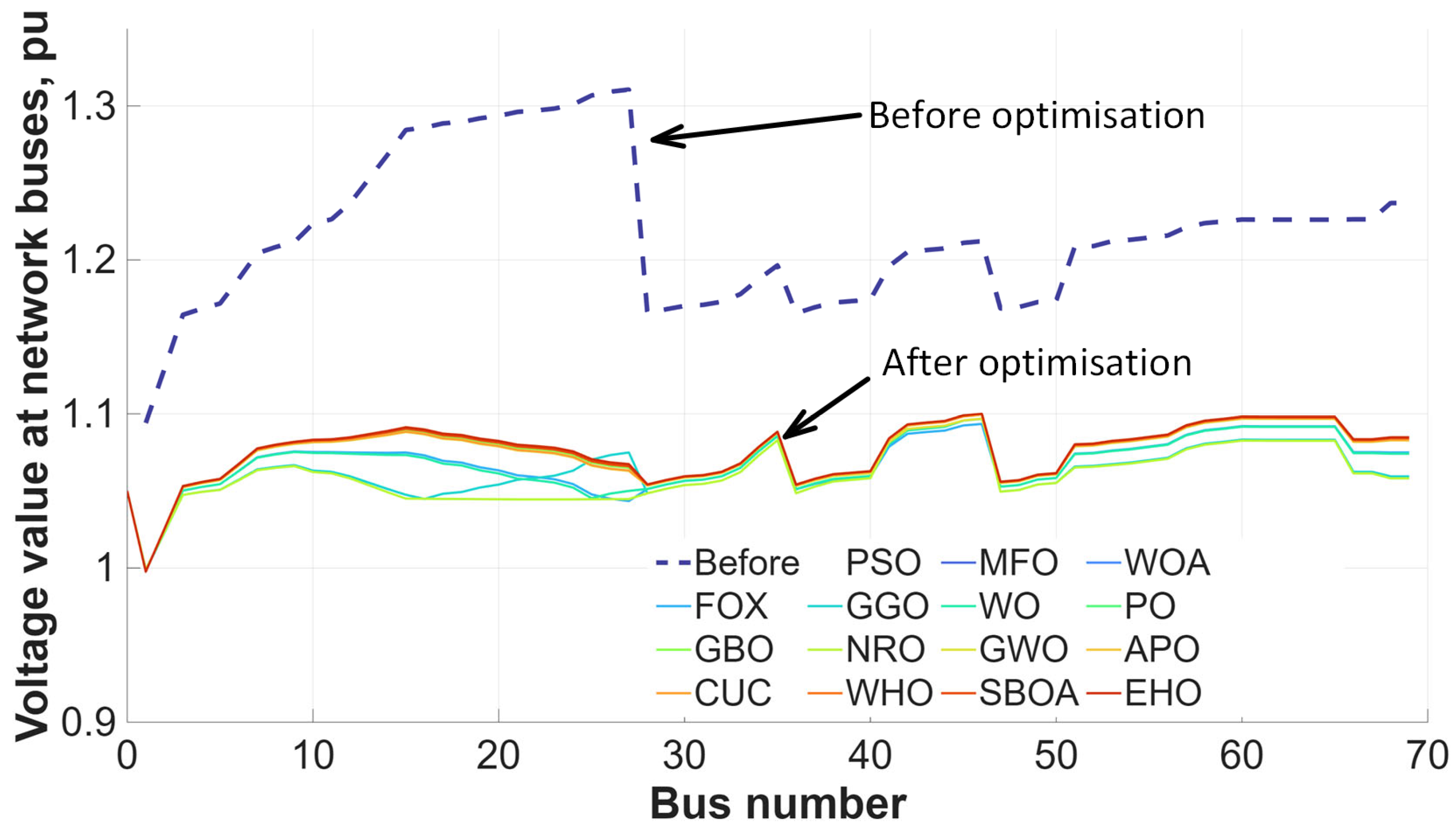
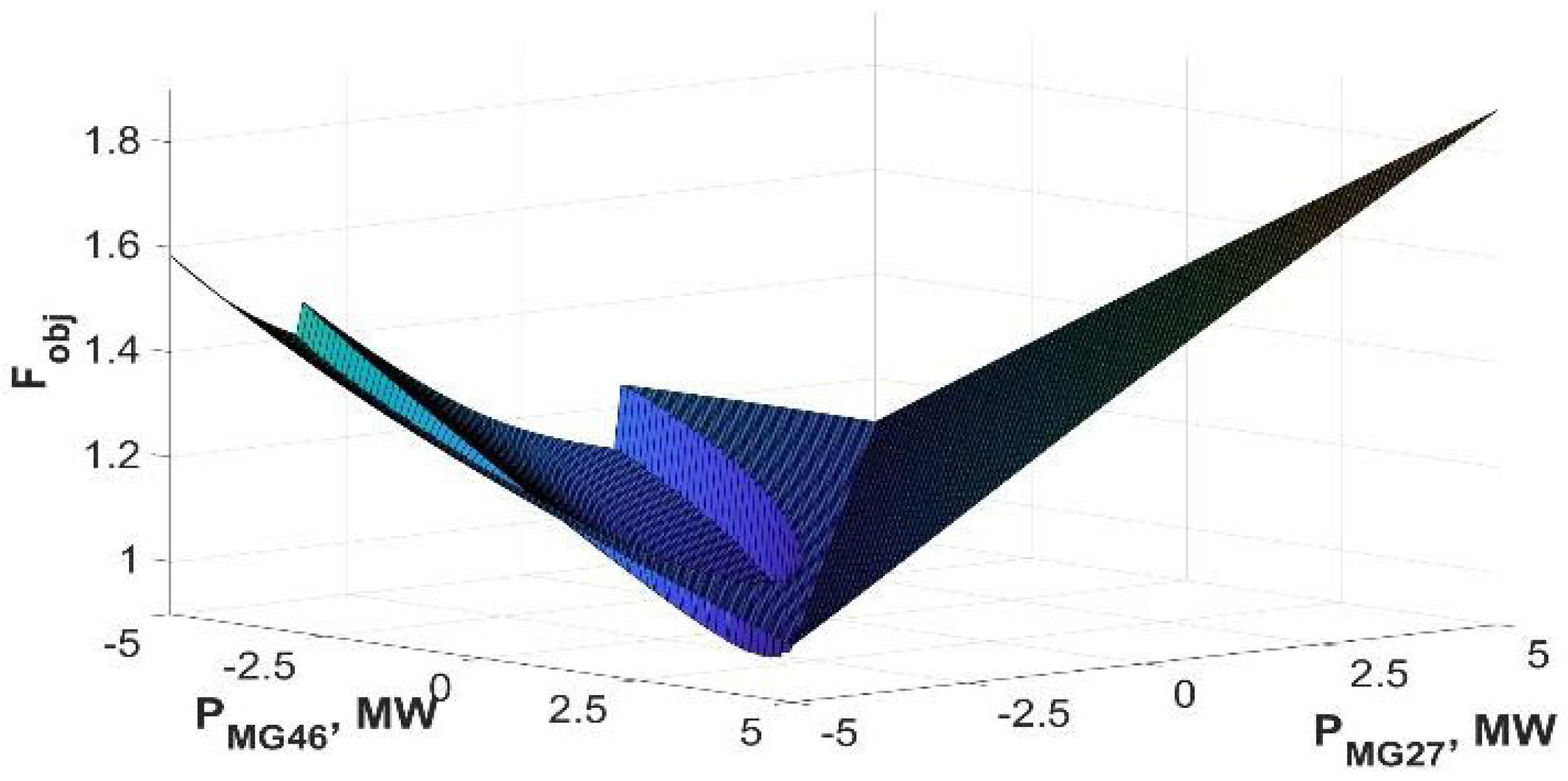
EHO	01:12:12	0.45781471	22	12	3.89	0.56

reports the best optimisation outcomes for F_obj1 in the case without IPC, including the selected ES locations and their power set-points. The performance of the considered metaheuristics is compared in Figure 5, while Figure 6 shows how quickly each method converges towards its final solution. Figure 7 shows voltage values in the network nodes. To better understand why population-based methods are suitable here, Figure 8 presents the response surface of F_obj1, which reveals a nonlinear objective landscape with a distinct near-optimal region.

Among the analysed optimisation methods, the best results, presented collectively in Table 2, were obtained for algorithms that achieved the objective-function values (F_obj1) in the range of about 0.44012–0.44017, i.e., the PSO, MFO, WO, PO, GWO, as well as WHO and SBOA methods. The lowest value of the objective function (F_obj1), described by the relation number (1), was achieved by the PO method (0.440120791), followed closely by WHO (0.440123037) and MFO (0.440138573). This means that these three methods provide the best optimisation quality in terms of minimising the objective function. In terms of time efficiency, most of the algorithms completed the calculations in the range of 1 h 12 min to 1 h 23 min, which is advantageous from the point of view of practical applications. However, some methods required much longer time (from about 2 to 4 h), which may be a limitation in dynamic operating environments. In terms of execution time, the fastest method was EHO (01:12:12), followed by MFO (01:12:36) and PSO (01:16:50), which suggests their high computational efficiency. In turn, the longest computational time was taken by the APO method (04:15:11).

Considering the trade-off between solution quality and runtime, MFO achieves a low objective value with short computation time, making it one of the most efficient methods tested. The PO method (0.440120791, 01:20:18) achieved the best objective function but at the cost of a slightly longer computational time.

5.2. Selection of the Location and Power of Two Energy Storage Facilities with the Possibility of an Emergency Increase in Power Consumption by Two Industrial Plants

The analyses performed in this section are aimed at determining the location and capacity of two energy storage facilities in the MV network. Unlike in Section 5.1, two additional loads (connected at nodes 15 and 60) operating in the DSM (Demand Side Management) service have been taken into account.

Table 3. Results for F_obj1 with IPC.

Method	Time	Fobj	ES1	ES2	PES1	PES2	PLD15	PLD60
	h	-	Bus nr.	Bus nr.	MW	MW	MW	MW
PSO	01:13:50	0.1465	21	36	1.67	0	2	1.0
MFO	01:15:36	0.1139	26	69	1.03	0	2	1
WOA	01:17:52	0.1294	27	50	1.19	0	2	0.5
FOX	01:19:18	0.1235	27	17	1.16	0	2	1
GGO	01:20:21	0.1920	20	65	2.28	0.61	1.1	0.6
WO	01:22:40	0.1202	27	19	1.08	0	2	1
PO	01:23:18	0.1139	27	6	1.03	0	2	1
GBO	01:23:39	0.1139	27	2	1.03	0	2	1
NRO	01:25:23	0.1141	26	2	1.03	0	2	1
GWO	01:24:07	0.1140	26	19	1.03	0	2	1
APO	04:03:11	0.1139	26	23	1.03	0	2	1.0
CUC	03:38:37	0.1140	27	12	1.03	0	2	1.0
WHO	02:46:40	0.1470	22	4	1.66	0	2	1
SBOA	02:36:13	0.1468	22	1	1.65	0	2	1
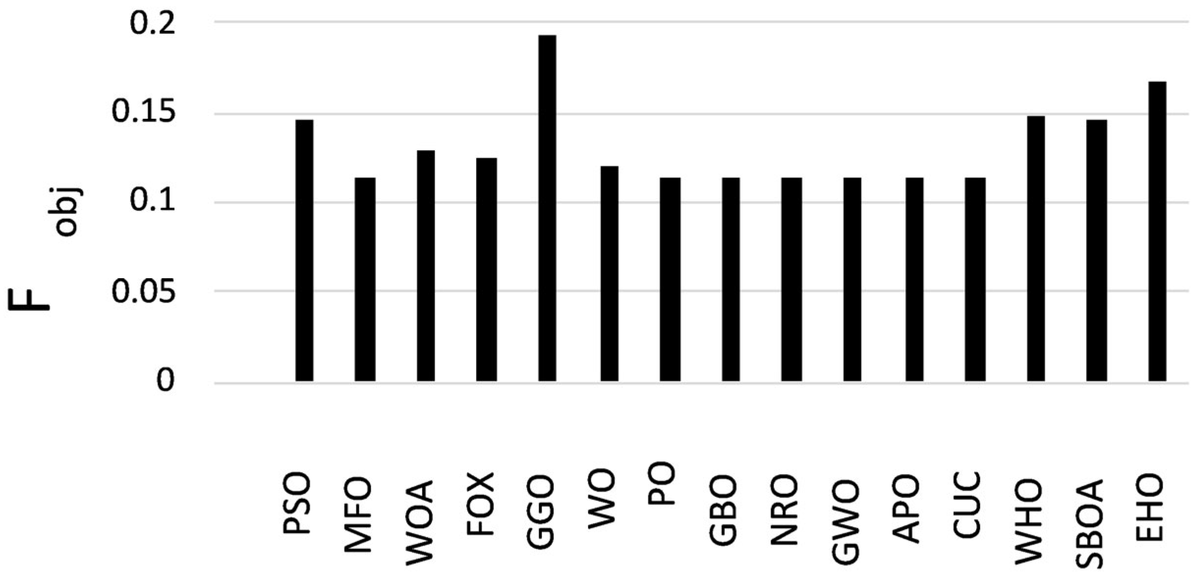
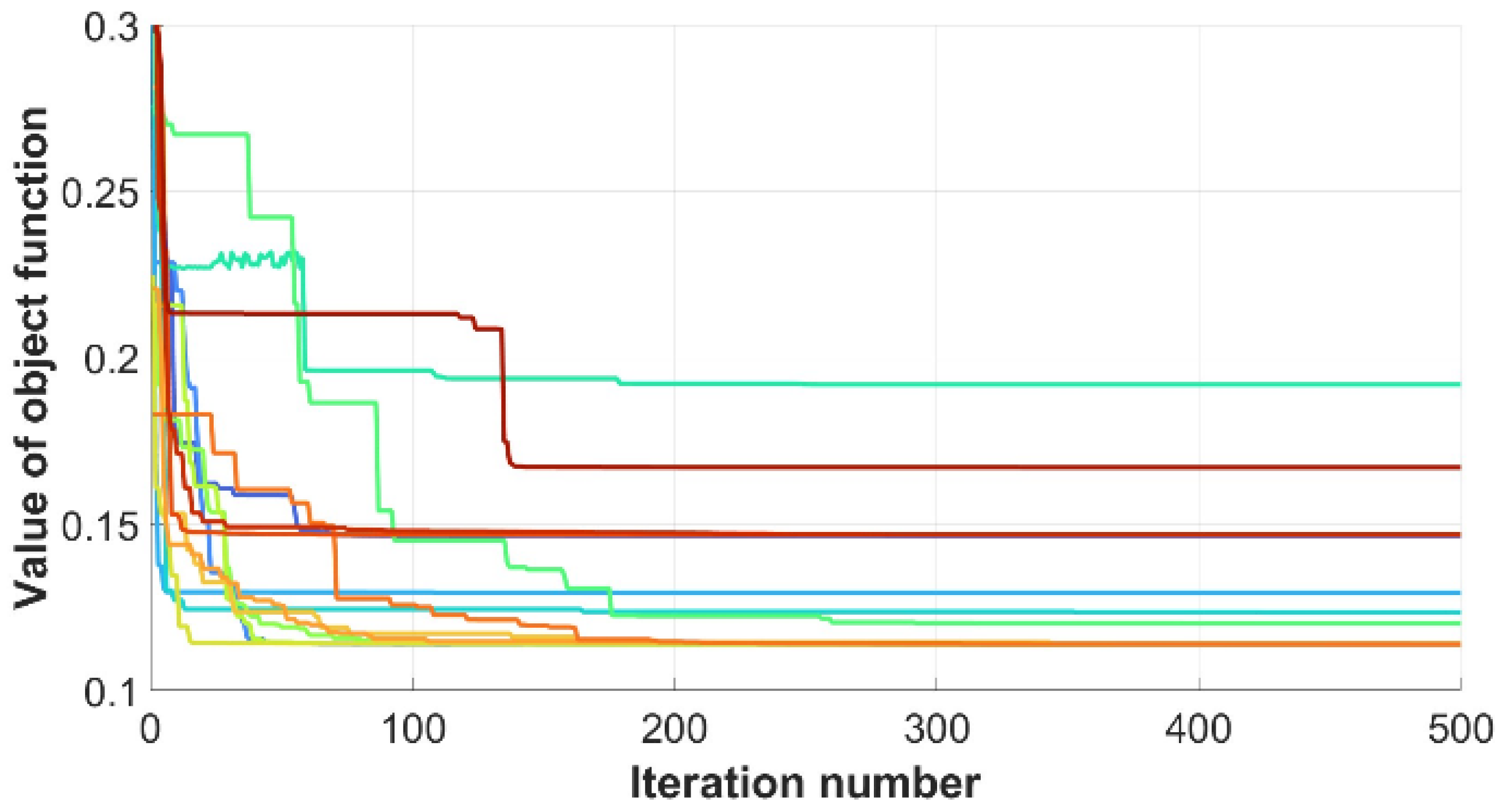
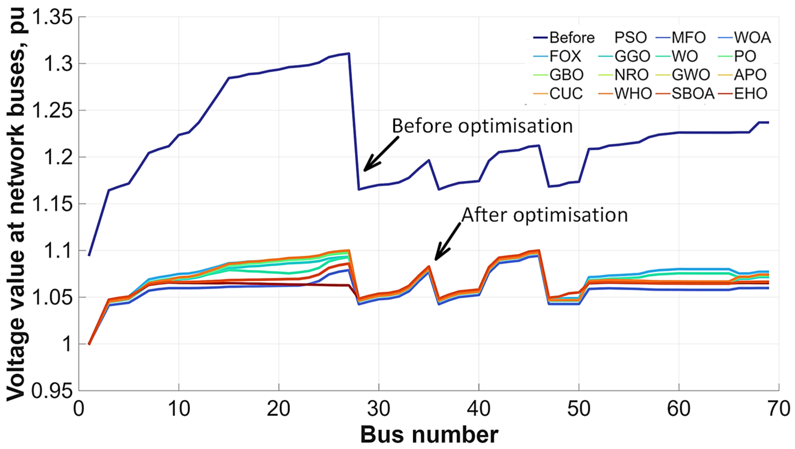
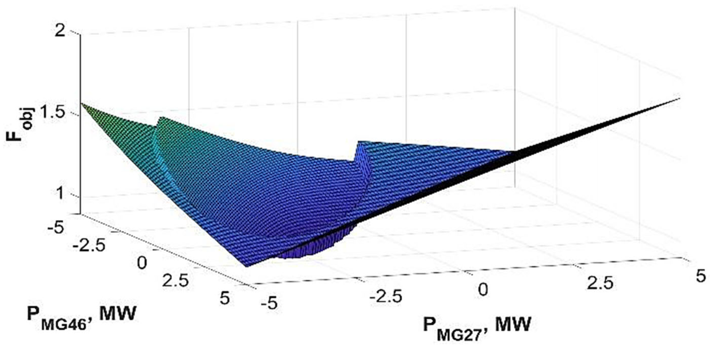
EHO	01:18:19	0.1671	27	66	2.04	0	1.8	1.0

summarises the best solutions obtained for F_obj1 when IPC is available, including the selected ES locations/powers and the IPC levels at buses 15 and 60. The accompanying figures provide complementary insight: Figure 9 compares the final objective values across the tested algorithms, whereas Figure 10 illustrates their convergence behaviour over iterations. The operational impact of the best solutions is reflected in the voltage profiles in Figure 11. Finally, Figure 12 visualises the objective landscape under IPC, highlighting the nonlinearity of F_obj1 and the region of near-optimal solutions.

The lowest values of the objective function, presented collectively in Table 3, were obtained by the MFO (0.1138), PO (0.1138), GBO (0.1138) and APO (0.1138) methods. However, the differences between them are so small that in practice they can be considered similar in terms of solution quality. The PSO, WOA, FOX, WHO, SBOA, EHO and GGO methods obtained higher objective-function values than those listed above, which indicates slightly worse optimisation efficiency in this scenario. In terms of computational time (excluding extremely long runs), the MFO (01:15:36), WO (01:22:40), PO (01:23:18), GBO (01:23:39) and GWO (01:24:07) methods are in a similar range of about 1 h 15–25 min, which is relatively short for a complex optimisation task. Some algorithms, such as APO (04:03:11) or CUC (03:38:37), despite good objective-function values, require significantly longer computational time, which may be a limitation in practical applications (e.g., when frequent updates of settings are required).

The simulation results for the objective function (1), including the selection of the location and power of installed energy storage facilities with the possibility of an interventional increase in power consumption by two industrial plants, showed a significant improvement in all the analysed indicators. Both the voltage coefficient, the power loss coefficient and the storage installation cost coefficient achieved more favourable values compared to the variant without interventional power consumption control. Thanks to the increase in the power of the receivers, it was possible to significantly reduce the required power of the energy storage facilities. Their total power dropped from 3.5 MW to only 1 MW. This indicates more efficient use of the existing infrastructure and improved local balancing, thereby reducing the required ES capacity and potentially lowering investment costs while maintaining acceptable operating conditions.

Based on the calculation results obtained, it was concluded that the best metaheuristic method (among the 15 algorithms used) is the PO method. Therefore, this method was used in further calculations.

5.3. Optimal Selection of Renewable Energy Sources and Energy Storage Facilities

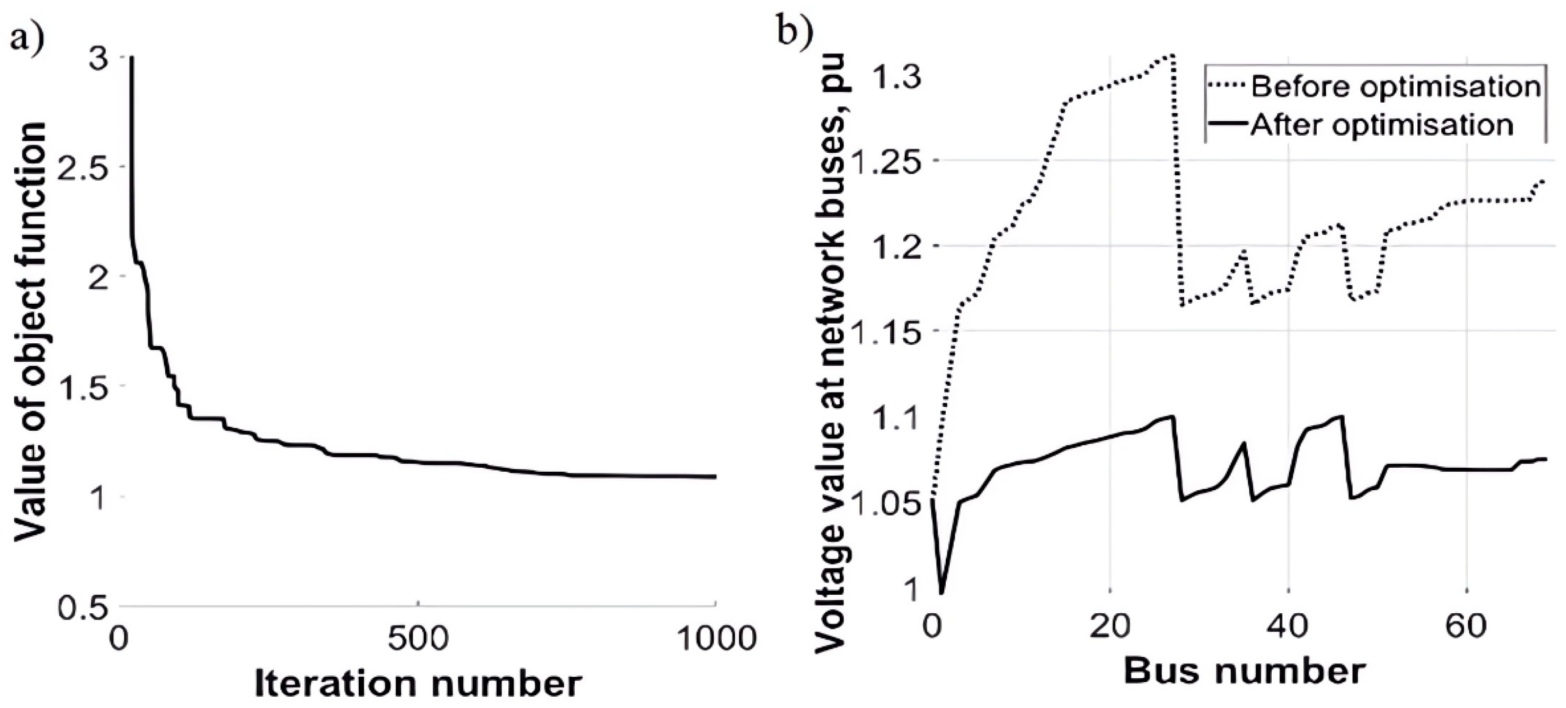
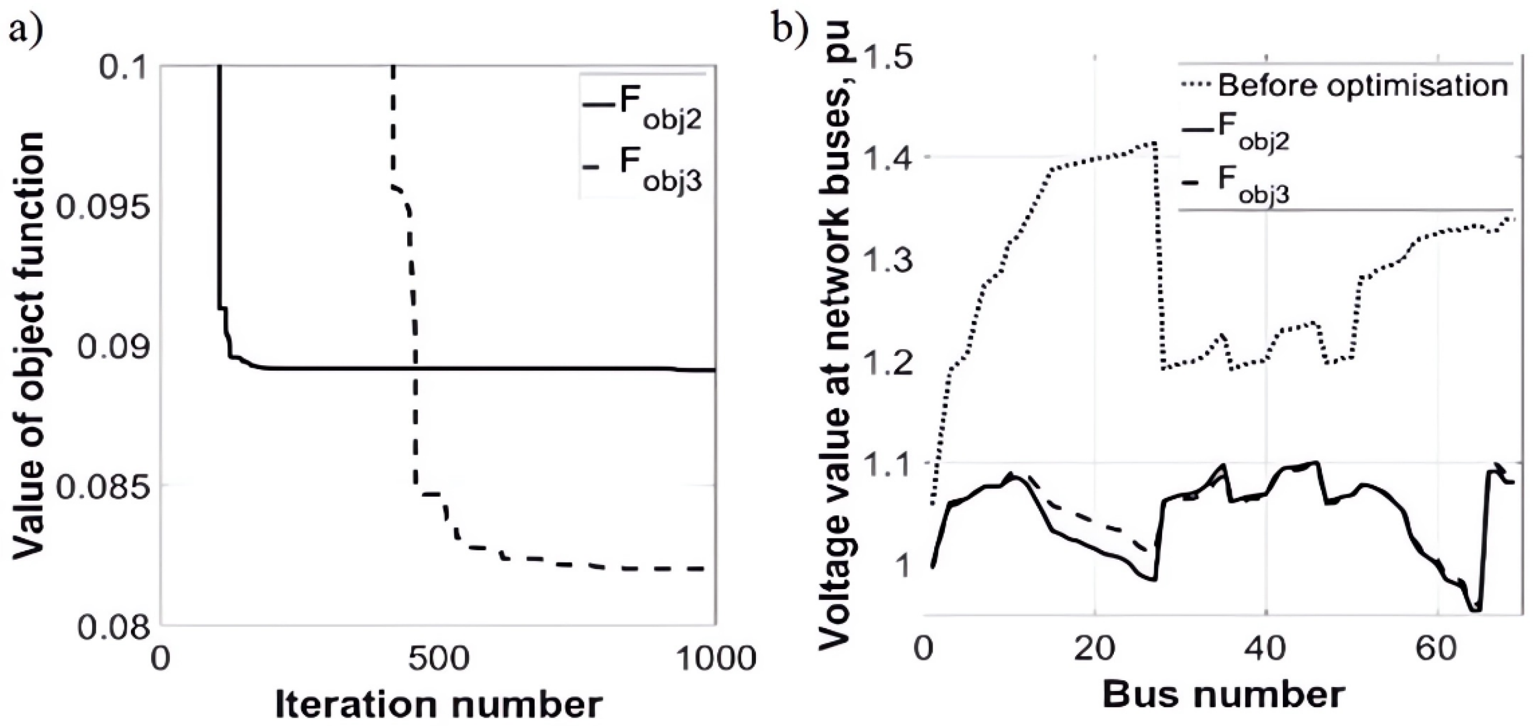
This subsection determines the maximum hosting capacity based on the second objective function (F_obj2). For this purpose, the possibility of connecting new PV sources in other network nodes was assumed. The results for F_obj2 are illustrated from two perspectives. Figure 13 shows the optimisation trajectory together with the resulting voltage profiles, which allows assessing how increased PV utilisation influences network operating limits. 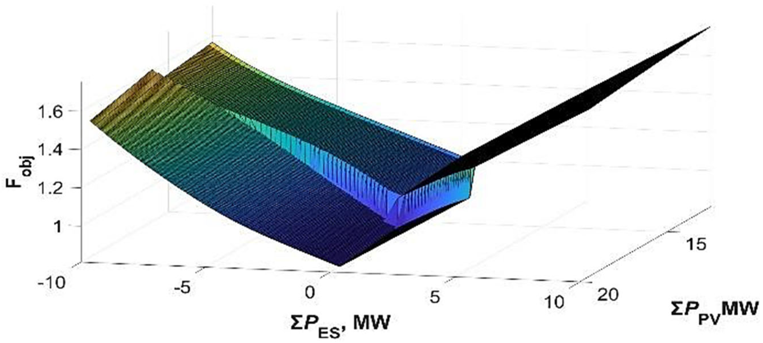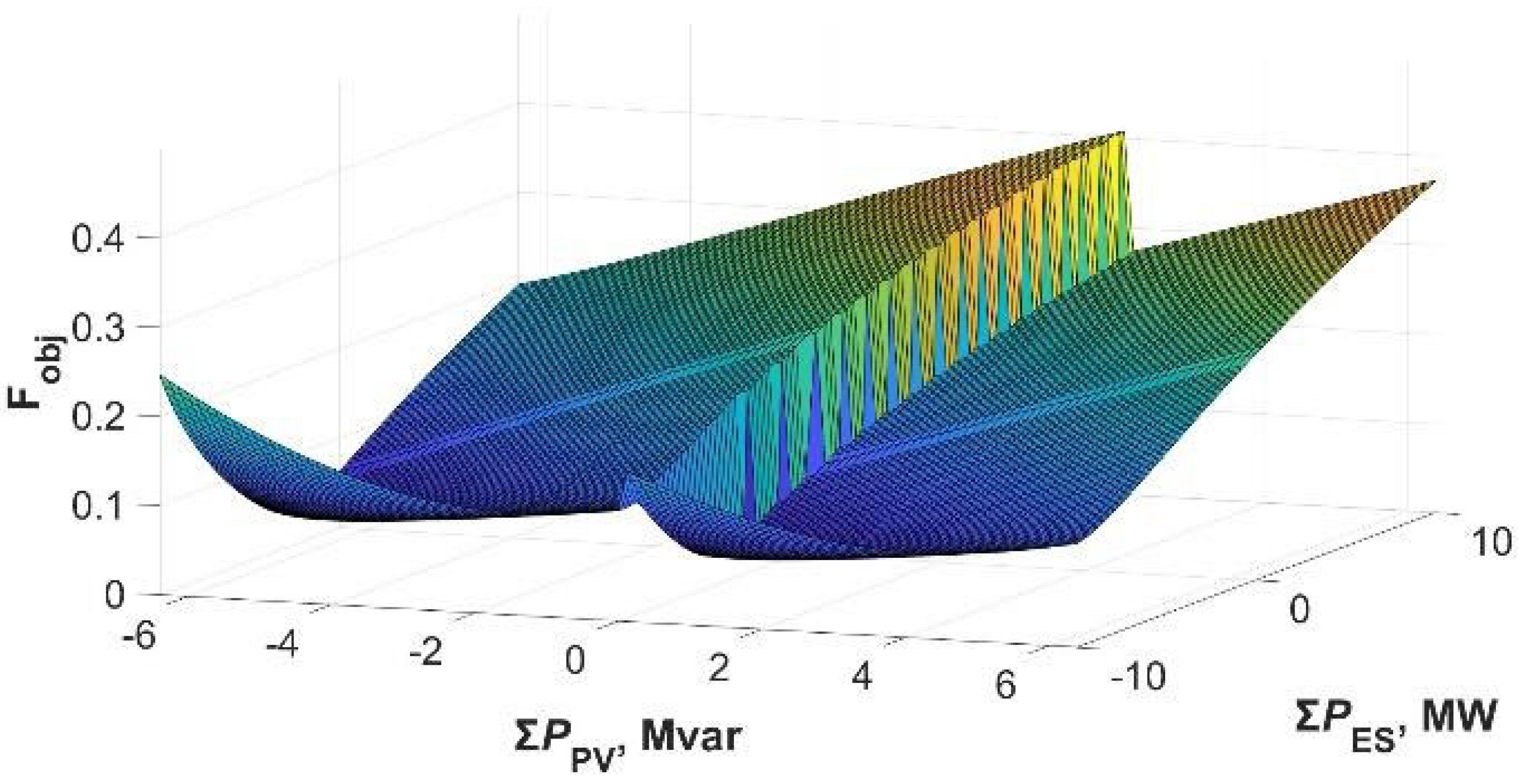In turn, Figure 14 provides a response-surface view of F_obj2 versus the aggregated PV and ES decision variables, highlighting the trade-off between higher RES penetration and the flexibility required from storage.

In the second objective function (8), the optimisation of the layout and active and reactive power of additional photovoltaic sources was also considered. The capacity of the power grid became an important factor, assessed in terms of the maximum possible connection capacity of renewable energy sources without compromising the stability of the system. The optimisation allowed the active power of the installed photovoltaic sources to be increased from 12.5 MW to 15.9 MW, which was possible thanks to the addition of a new PV installation with a capacity of 3.4 MW in node no. 1. The results indicate an improvement in the efficiency of the use of the network infrastructure, enabling greater penetration of RESs while maintaining the permissible operating parameters of the medium-voltage network.

5.4. Maximum Utilisation of the Power Hosting Capacity

The analyses carried out in this subsection were aimed at determining the maximum hosting capacity based on the third objective function (F_obj3). For this purpose, the possibility of connecting new PV sources in all network nodes was assumed. For the hosting-capacity objective F_obj3, Figure 15 presents the convergence of the optimisation and the corresponding voltage profiles for the best solution, providing a direct view of feasibility under increased PV installation. Complementarily, Figure 16 visualises the objective surface as a function of the aggregated PV and ES capacities, which helps to interpret the feasible region enabling maximal PV hosting within the adopted constraints.

For the third objective function, aimed at maximising PV hosting capacity, a total installed PV capacity of 26.4 MW was obtained. The optimisation distributed PV generation across the network buses, with the largest single PV unit reaching 2.1 MW. The average power of the 16 newly selected PV sources was 0.87 MW. These results indicate increased ability of the network to accommodate additional RESs while keeping voltages and loadings within admissible limits in the considered case study.

5.5. Optimisation of Network Operation with Selected Elements

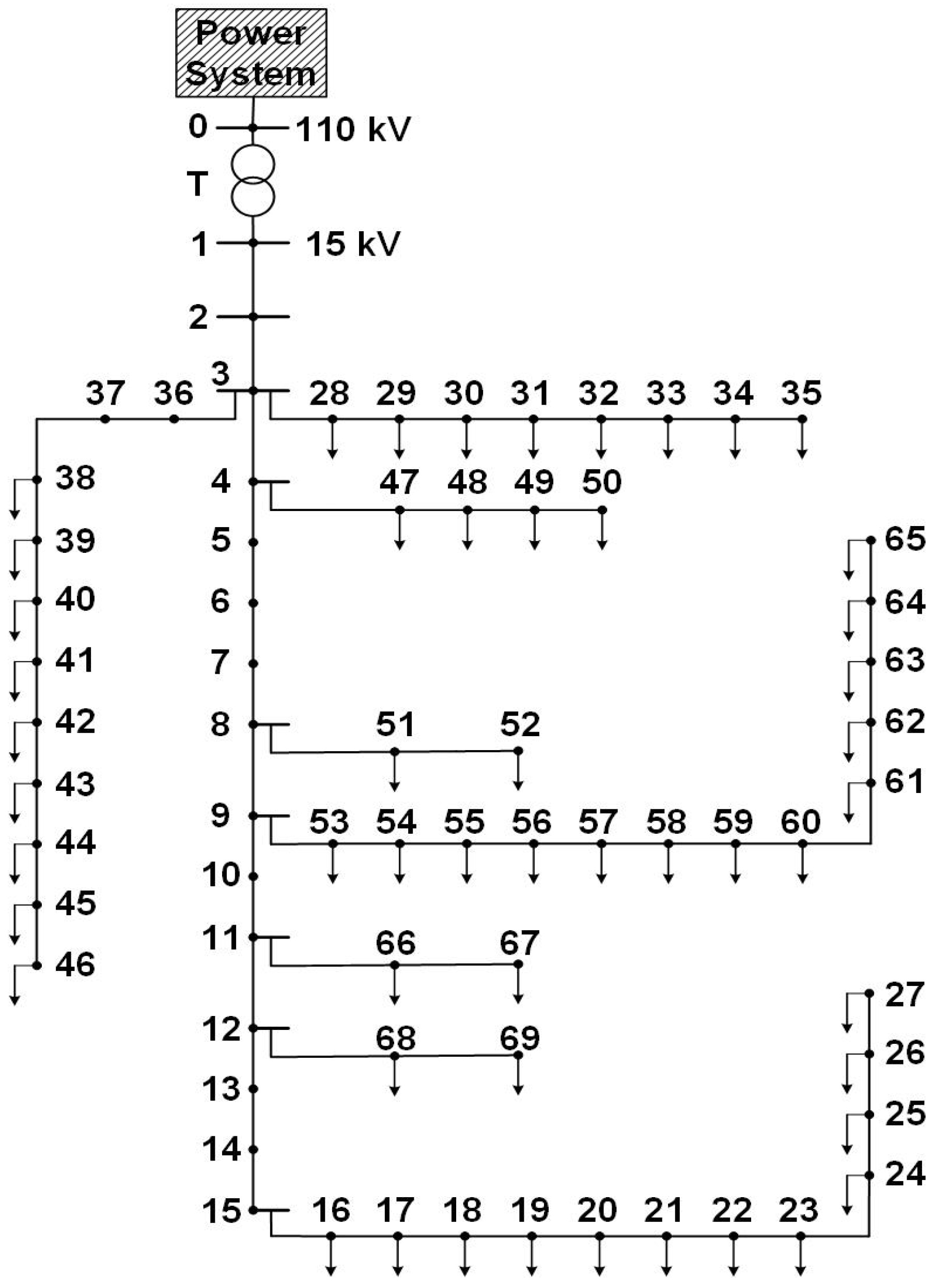
The optimisation calculations in this subsection concern the fourth objective function (F_obj4), which has two components. The first element concerns power losses, and the second is a voltage indicator. The form of this function is intended to reflect the actual operational requirements of network operators. The analyses were aimed at minimising the objective function. The results of the calculations obtained in the previous subsections were used for this purpose. It was assumed that energy storage facilities would be connected at nodes 27 and 46 and new sources at nodes 1, 9, 15, 27, 35, 46, 52 and 60. Two loads connected at nodes 15 and 60 as part of the DSM service were also taken into account.

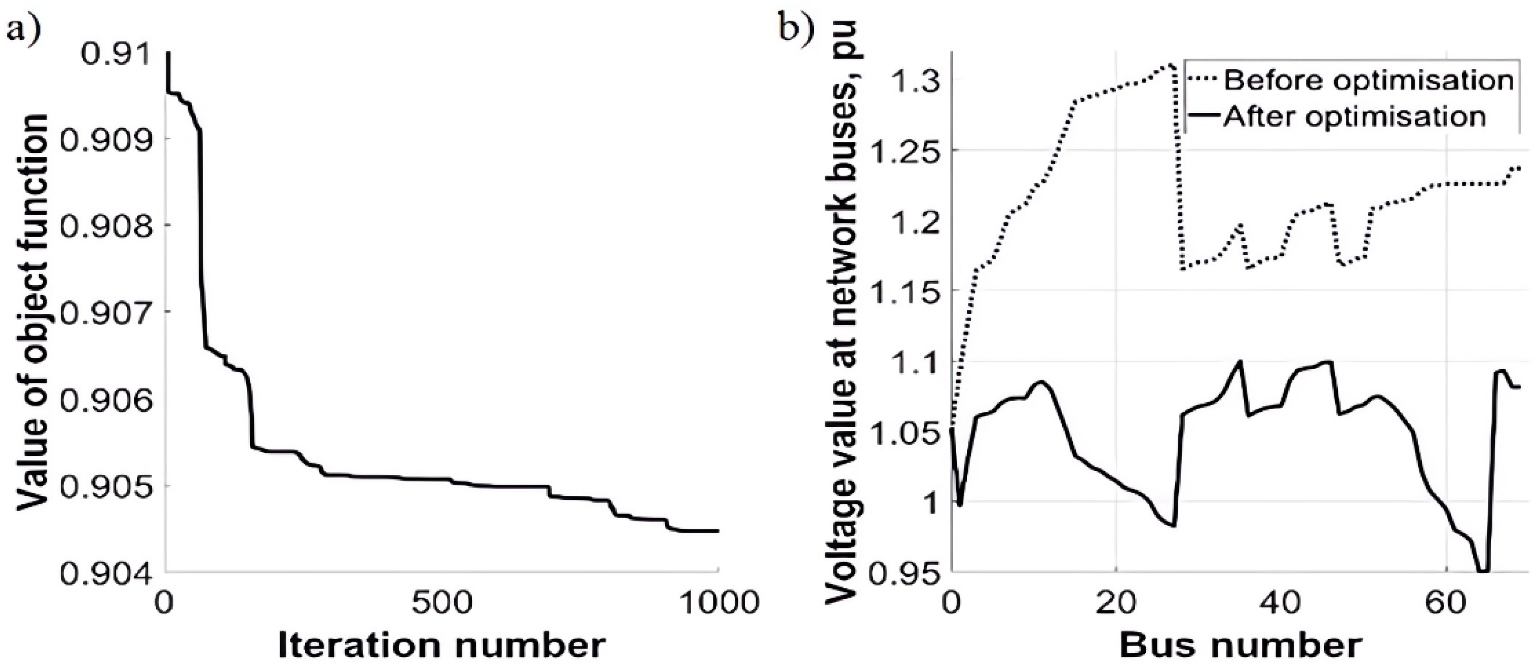
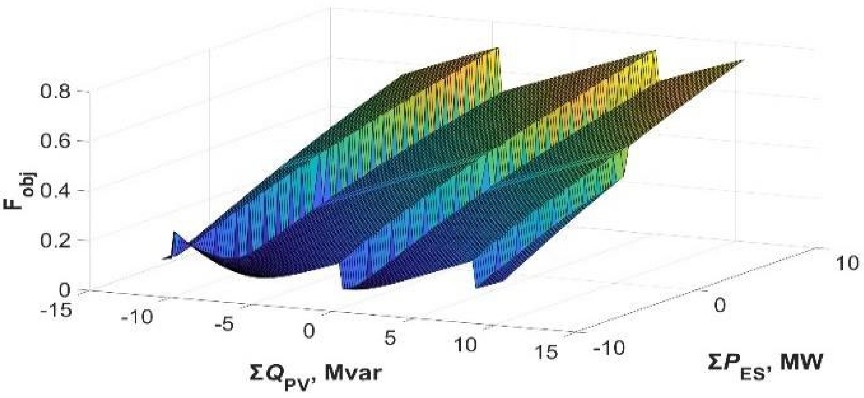
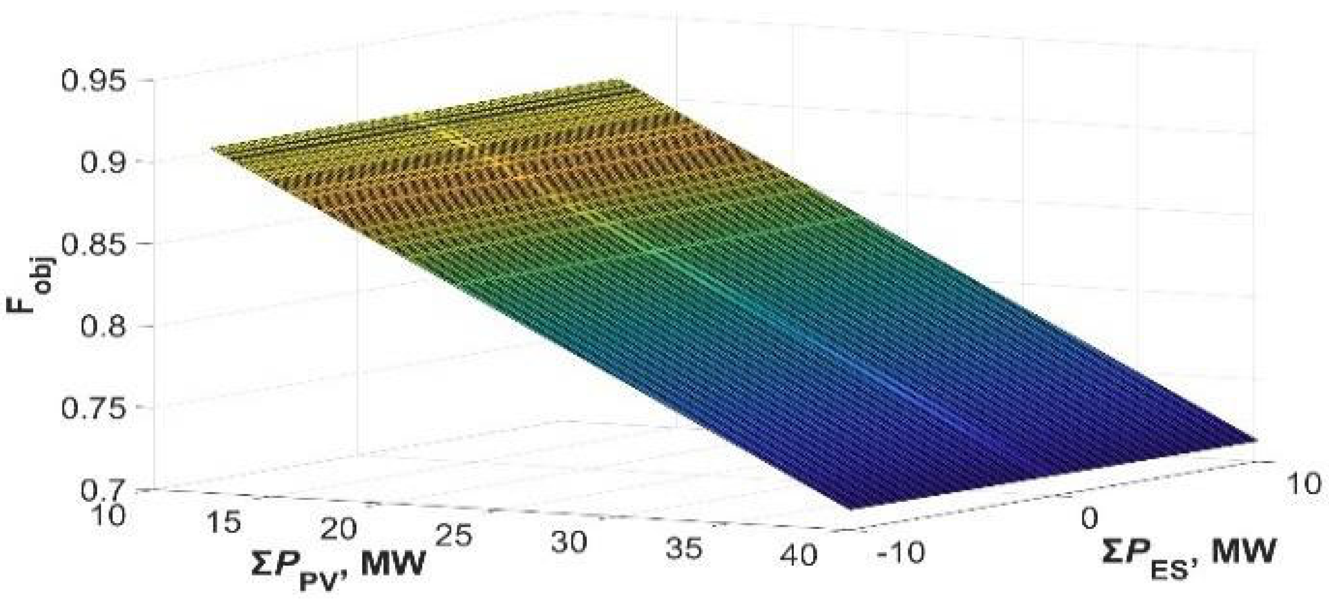
Stage 2 is illustrated in Figure 17, which shows the optimisation progress of F_obj4 and the resulting voltage profile after the final refinement. The objective landscapes in Figure 18 and Figure 19 further explain the sensitivity of F_obj4 to the tuned operating set-points for configurations inherited from Stage 1 (derived from F_obj2 and F_obj3, respectively). This presentation clarifies how operational tuning improves indices without changing the previously selected PV/ES placement.

The last objective function (11) was used to analyse the possibilities of further improving the network operation parameters by regulating the power of energy storage devices, controlling the power of interventional loads and adjusting the reactive power of photovoltaic sources. The goal was to achieve the best possible values of the voltage index and the power loss index with the previously optimised structure of PV source and storage locations. The results show that, although the obtained parameters were similar to the previous optimisation steps, it was possible to achieve an improvement in the voltage index and the level of power losses. These results indicate that the proposed final tuning stage can further improve voltage and loss indices for a fixed configuration obtained in Stage 1. In practical applications, such refinement may be used as an additional adjustment step when updated set-points are required without changing previously selected PV/ES placements.

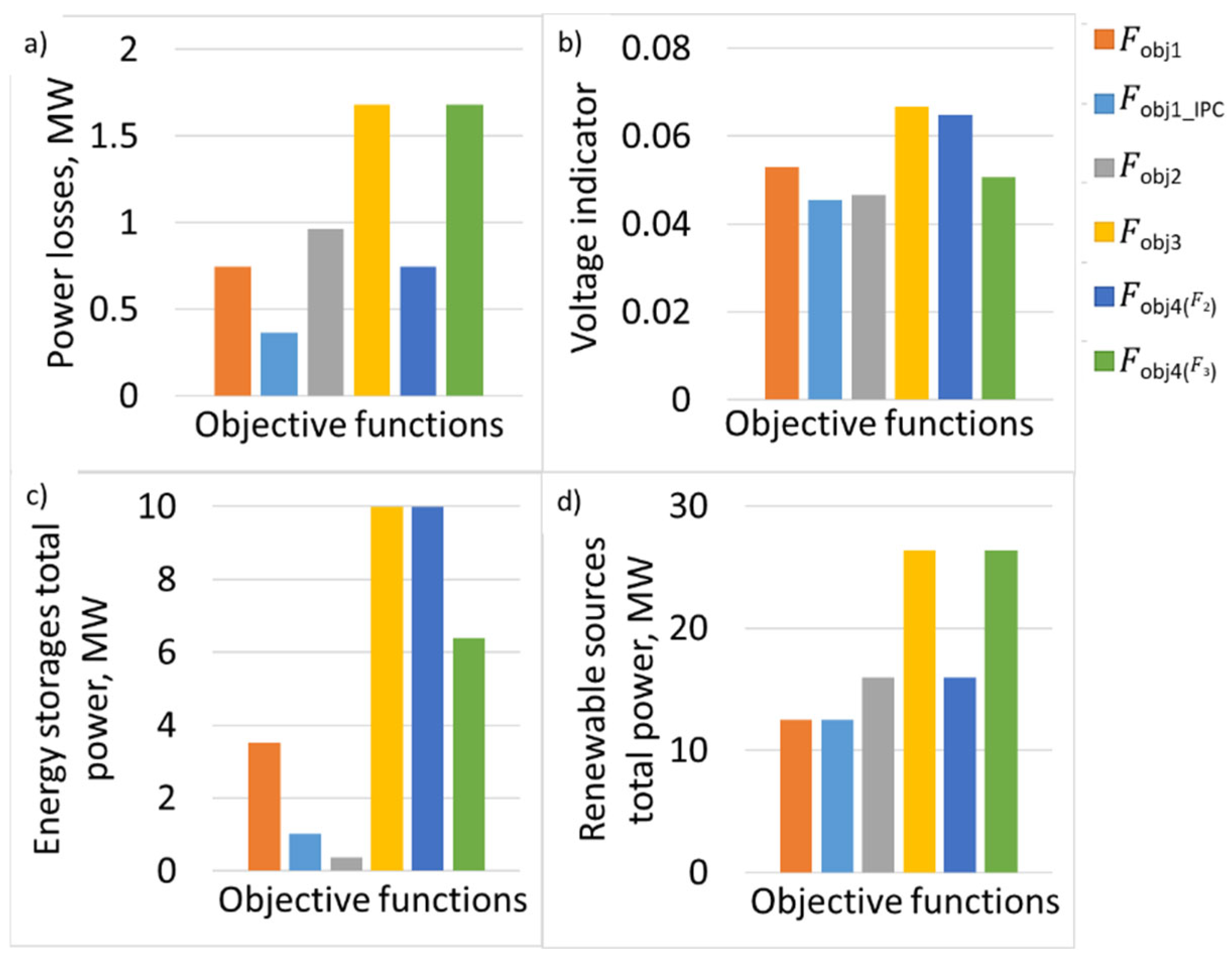
Figure 20 provides a compact comparison of the outcomes obtained in successive optimisation stages: F_obj1 (with and without IPC), F_obj2, F_obj3, and the final refinement F_obj4 applied to configurations derived from F_obj2 and F_obj3. The subplots summarise how the key indicators—relative losses dP_loss, voltage deviation U_dev, total storage power ∑P_ES, and total PV power ∑P_PV—evolve as the operator priorities shift between stages. This comparison helps to interpret the practical trade-offs and supports selecting the most suitable objective formulation for a given operational goal.

6. Conclusions

In the considered case study, introducing IPC for two industrial plants improved the main operating indices, reducing losses and mitigating voltage issues while lowering the required total ES power from 3.5 MW to 1 MW under the adopted operating scenario. Optimisation of storage location and regulation of the reactive power of inverters enabled increasing the power of connected photovoltaic sources from 12.5 MW to 15.9 MW while maintaining network stability. In the next step, by maximising the use of network capacity, it was possible to almost double the power of installed PV sources to 26.4 MW, with the largest single source having a power of 2.1 MW and an average power of 0.87 MW per installation. Additional optimisation of network operation parameters, consisting of adjusting storage dispatch and controllable loads and controlling the reactive power of PV, led to a further, although small, improvement in voltage and power losses.

The simulations indicate that metaheuristic optimisation is a suitable approach for the considered MV case study. Among the tested methods, MFO, PO and GBO achieved the best (or comparable) objective values with relatively short computation times under the same computational budget. An important aspect was also the appropriate configuration of the objective-function weights, allowing for precise adjustment of optimisation priorities. The introduction of IPC reduces the required ES power in the considered scenarios, which may translate into lower investment needs and improved operational flexibility depending on the implementation and market conditions. The results of the analyses indicate that intelligent load control, optimisation of the distribution of RESs and reactive power regulation enable significant improvements in medium-voltage network operation while increasing its ability to integrate RESs.

The novelty of this work lies in proposing four original objective-function formulations reflecting different operator priorities and evaluating them within a unified MATLAB–PowerFactory co-simulation framework. In addition, a comparative study of 15 optimisation algorithms is provided under a consistent computational budget, which offers a practical reference for selecting suitable metaheuristics for similar MV optimisation tasks.

In future research, the authors plan to use methods based on artificial intelligence, using the results obtained in the optimisation processes as input data. Integration of AI algorithms with existing solutions would significantly shorten parameter selection time and increase the efficiency of the entire optimisation process, which may contribute to an even better adaptation of the power grid to dynamic operating conditions [41].