High-Resolution Spatiotemporal Carbon Emission Estimation in Northeast China Based on XGBoost and Multi-Source Data

Abstract

Accurately characterizing spatiotemporal patterns of carbon emissions and their driving mechanisms is essential for advancing regional low-carbon transitions. Focusing on northeast China, a representative old industrial base, this study develops a spatialized carbon emission estimation framework using an XGBoost model that integrates nighttime light data, land-use information, population, and economic indicators. A 1 km resolution carbon emission dataset spanning 2000 to 2021 is generated, and the SHAP method reveals nonlinear responses and stage-dependent evolutions of key driving factors. The results demonstrate three key findings. Carbon emissions in northeast China increased from 636 Mt in 2000 to 1131 Mt in 2021, exhibiting three distinct phases: rapid expansion (2000–2010, +36%), peak stabilization (2010–2015, +13%), and localized contraction (2015–2021, +3%). Liaoning Province contributed 46% of total emissions in 2021, while Jilin showed the fastest growth rate at 92%. County-level Moran’s I values (0.292–0.349) remain substantially lower than city-level values (0.642–0.700), revealing scale-dependent spatial clustering. High–high clusters concentrated persistently in southern Liaoning, encompassing eight cities by 2010, whereas low–low clusters dominated northern Heilongjiang. Population and GDP exhibited saturating marginal effects after 2015, with SHAP values plateauing beyond thresholds of approximately 450,000 persons and 420 billion CNY respectively, indicating gradual decoupling between economic growth and emissions. Industrial mining land influence declined by 68% from 2005 to 2020, while urban land-use ratio maintained stable contributions. This high-resolution spatiotemporal dataset provides empirical evidence for designing threshold-based emission reduction policies, identifying regional transfer risks, and implementing county-level differentiated strategies in old industrial bases undergoing low-carbon transition. The XGBoost–SHAP framework demonstrates transferability to other heavy industrial regions facing similar structural transformation challenges.

1. Introduction

With the continued expansion of global economic activities, deepening industrialization, and rapid growth of energy consumption, anthropogenic activities have become the dominant driver of sharp increases in atmospheric carbon dioxide concentrations [1,2]. In 2021, China’s energy-related carbon emissions (CE) reached 10.52 billion tons, accounting for 31.1% of the global total [3] and ranking first worldwide [4]. Addressing climate change has thus become a global consensus. Recent advances in emission reduction encompass optimization of energy systems, carbon capture deployment, and integrated assessment modeling, providing complementary perspectives for understanding mitigation pathways. Under the Paris Agreement, parties are required to regularly update their Nationally Determined Contributions (NDCs) to progressively strengthen mitigation commitments. In this context, China has announced its dual carbon goals: peaking carbon emissions before 2030 and achieving carbon neutrality by 2060. These targets signal a fundamental shift in China’s development paradigm from high-carbon dependence toward low-carbon transformation [5,6,7].

Advancing a systematic low-carbon transition under the “carbon peaking–carbon neutrality” framework places higher demands on the spatiotemporal precision of CE accounting and the policy relevance of regional analyses [8,9,10,11,12]. Compared with aggregate national or provincial inventories, the core challenge of regional carbon governance lies in identifying spatial heterogeneity, clustering structures, and stage-dependent dynamics of CE at finer spatial and temporal scales, and further uncovering the nonlinear responses and interaction mechanisms among driving factors. Such analyses are essential for building a robust and verifiable evidence base to support differentiated mitigation policies.

Northeast China, as a typical old industrial base and energy-intensive region, has long served as a key hub for heavy industries such as steel, energy, chemicals, and equipment manufacturing [13]. Owing to the coal-dominated energy structure, prolonged heating periods, and strong industrial path dependence, this region exhibits persistently high emission intensities and pronounced lock-in effects. Existing studies have also highlighted the increasing constraints associated with emission peaking and the mounting pressure for structural transformation in northeast China [14]. Therefore, constructing high-resolution, long-term spatialized carbon emission datasets and systematically analyzing their driving mechanisms constitute a critical foundation for identifying key constraints and policy leverage points in the regional low-carbon transition. However, most existing emission estimates rely on statistical or inventory-based data, which, while effective for capturing macro-level trends, are often limited by coarse spatial resolution, missing spatial information, and delayed updates, thereby constraining their applicability for refined governance and targeted policy design [15].

In recent years, nighttime light data have been widely employed in spatializing CE due to their ability to proxy human activity intensity, demonstrating considerable potential across multiple spatial scales [16,17]. Nevertheless, as an integrated proxy indicator, NTL alone cannot adequately reveal the underlying socioeconomic mechanisms driving CE. The structural bias known as “similar brightness but different emissions” further limits its explanatory power [18]. Moreover, the relationships between driving factors and CE are often characterized by nonlinear features, including thresholds, saturation effects, and higher-order interactions, which are difficult to capture using simple linear assumptions or traditional parametric models. To improve estimation accuracy and enhance mechanism interpretation, recent studies have increasingly incorporated multi-source data such as land-use, population, and economic indicators [19,20,21]. However, many of these efforts still rely on linear or weakly nonlinear frameworks, providing limited insight into the nonlinear contributions, stage-dependent evolution, and synergistic or antagonistic interactions among driving factors.

For predictive tasks involving complex spatial parameters, gradient boosting decision tree models, particularly XGBoost, offer strong capabilities in handling nonlinear relationships and feature interactions. Compared with neural networks, which are often criticized as black boxes, or random forest models, XGBoost exhibits distinct advantages in balancing predictive performance and model robustness under such conditions [22,23]. When combined with the SHAP interpretability framework, model outputs can be decomposed into feature-level contributions, enabling mechanism-oriented interpretation while maintaining high predictive accuracy [24,25]. Nevertheless, from the perspectives of study region and data products, existing research on carbon emissions has predominantly focused on international [26], national, provincial, and city scales [27,28]. Long-term, high-resolution carbon emission datasets for typical heavy industrial regions such as northeast China remain relatively scarce. Furthermore, few studies have achieved a closed-loop analytical framework that simultaneously integrates high-precision estimation, multi-scale spatial pattern characterization, and nonlinear mechanism interpretation. This gap constrains the accurate identification of key transformation bottlenecks and the formulation of differentiated mitigation strategies at the regional scale.

Existing gridded products such as ODIAC and EDGAR provide global coverage but face limitations in capturing subnational heterogeneity. ODIAC achieves 1 km resolution through point source databases and nighttime lights but exhibits limited temporal granularity and delayed updates. EDGAR offers sectoral decomposition at 0.1° resolution, yet this coarse-grained approach obscures county-level dynamics. Both employ top-down disaggregation that may not reflect local socioeconomic structures in rapidly transforming regions. The present study advances beyond these products by integrating population, land cover, and economic indicators into a machine learning framework, enabling bottom-up capture of emission drivers while maintaining high resolution. SHAP interpretability further allows mechanism-oriented analysis of nonlinear interactions, a capability not provided by conventional inventory products.

Against this background, this study develops a spatialized carbon emission estimation framework based on XGBoost, integrating multi-source spatial information including nighttime light (NTL), China Land Cover Dataset (CLCD), population (POP), and Gross Domestic Product (GDP). Using CE data as the training target, we generate a long-term (2000–2021), 1 km × 1 km resolution gridded carbon emission dataset for northeast China. The SHAP method is further employed to identify nonlinear responses, threshold effects, and interaction patterns among driving factors, while spatial clustering structures and scale effects of CE are examined at both city and county levels.

The main contributions of this study are threefold:

(1)

A CE spatialization framework integrating predictive accuracy and mechanistic interpretability is proposed, enabling high-resolution long-term estimation through multi-source data integration.

(2)

The spatial agglomeration patterns, path-dependent characteristics, and phased evolutionary trajectories of CE in northeast China are systematically characterized across municipal and county scales.

(3)

The nonlinear marginal effects and stage-specific mechanistic transitions of key driving factors are quantitatively identified, providing mechanistic evidence and spatial targeting for differentiated mitigation strategies in heavy industrial regions.

The paper proceeds as follows. Section 2 describes the study area and data sources. Section 3 presents methods including nighttime light preprocessing, XGBoost modeling, SHAP interpretation, and spatial analysis. Section 4 reports spatiotemporal evolution, clustering structures, and driving mechanisms. Section 5 discusses model performance, methodological limitations, and comparisons with existing products. Section 6 summarizes conclusions and policy implications.

2. Study Area and Data

2.1. Study Area

As China’s major heavy industrial base and one of its most energy-intensive regions, the three provinces of northeast China, which include Liaoning Province, Jilin Province, and Heilongjiang Province, are located in the northeastern part of the country, covering a total area of approximately 787,300 km². The region borders Russia to the north and east, adjoins North Korea to the southeast, connects to the Inner Mongolia Autonomous Region to the west, and faces the Bohai Sea and the Yellow Sea to the south, conferring a strategically significant geographic position [29,30]. Administratively, the region comprises 36 prefecture-level cities and 282 county-level units.

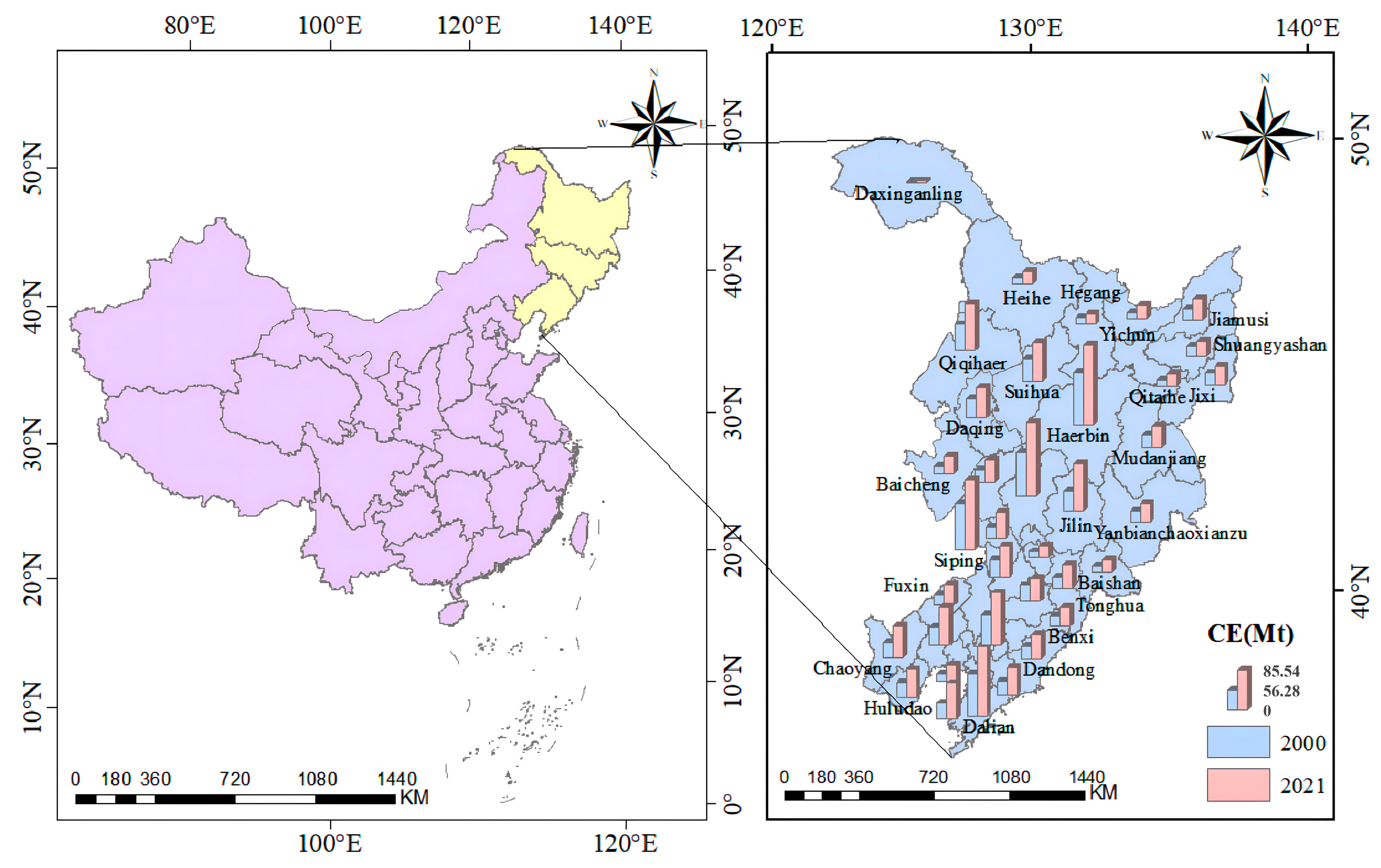
As shown in

Table 1. Socioeconomic and energy characteristics of northeast China provinces (2021).

Province	Area (km2)	Population (Million)	GDP (Billion CNY)	Secondary Sector (%)	Coal Share (%)	Heating Months	Dominant Industries
Liaoning	145,900	42.59	2789	39.1	58.7	5	Steel, petrochemicals, equipment
Jilin	187,400	24.07	1324	35.6	62.3	5.5	Automobiles, chemicals, food
Heilongjiang	454,000	31.85	1503	28.3	65.8	6	Petroleum, machinery, agriculture

, the three northeastern provinces are endowed with abundant mineral resources, particularly coal, iron ore, and petroleum, which have long underpinned a heavy industrial system dominated by steel production, machinery manufacturing, and chemical industries. The secondary sector accounts for 28–39% of regional GDP, substantially exceeding the national average. Energy consumption remains highly coal-dependent, with fossil fuels constituting 59–66% of total energy use. In addition, the region is subject to a cold continental climate, with winter heating periods lasting approximately five to six months, which further intensifies energy demand and consumption levels [31]. This combination of high resource input and high energy consumption has rendered northeast China one of the regions with the highest carbon emission intensity and the most severe challenges for emission reduction and low-carbon transition in China. Figure 1 illustrates the spatial distribution of city-level carbon emissions across the three northeastern provinces.

2.2. Data Sources

This study integrates multiple sources of spatial data to support the spatialized estimation of CE and the analysis of their driving mechanisms, including nighttime light observations, land-use information, population and economic data, as well as administrative boundary datasets.

NTL data consist of both the DMSP-OLS stable light products and the monthly composite NPP-VIIRS datasets [32,33], which together provide long-term continuity and enhanced radiometric sensitivity for characterizing human activity intensity. Land-use information is derived from the annual China Land Cover Dataset (CLCD) [34], offering consistent and temporally continuous land-cover classifications. Population data are obtained from the LandScan global population grid at a spatial resolution of 1 km [35]. Gridded GDP data are sourced from the Resource and Environmental Science and Data Center, which provides spatially explicit economic indicators suitable for regional-scale analysis [36]. Administrative boundary data are used to define spatial analysis units and to support multi-scale statistical and spatial autocorrelation analyses at the city and county levels. Carbon emission inventory data are obtained from the China Emission Accounts and Datasets (CEADs), specifically the city-level carbon emission inventory, which serves as the target variable for model training and validation [37], The data sources are summarized in

Table 2. Description of datasets used in this study.

Dataset	Spatial Resolution	Temporal Coverage	Data Format	Update Frequency	Data Volume	Access
DMSP-OLS Nighttime Light	~1 km	2000–2013 (annual)	GeoTIFF	Archived (discontinued)	14 files	https://ngdc.noaa.gov/eog/dmsp (accessed on 15 November 2024)
NPP-VIIRS Nighttime Light	500 m	2012–2021 (monthly composite)	HDF5	Monthly	120 files	https://eogdata.mines.edu/products/vnl (accessed on 15 November 2024)
CLCD Land Cover	30 m	2000–2021 (annual)	GeoTIFF	Annual	22 files (8 classes)	https://doi.org/10.5281/zenodo.5816591 (accessed on 15 November 2024)
LandScan Population	1 km	2000–2021 (annual)	GeoTIFF	Annual	22 files	https://landscan.ornl.gov (accessed on 15 November 2024)
Gridded GDP	1 km	2000–2020 (annual)	GeoTIFF	Annual	21 files	https://www.resdc.cn (accessed on 15 November 2024)
CEADs Emission Inventory	City-level (administrative)	2000–2021 (annual)	Excel/CSV	Annual	1 file (36 cities × 22 years)	https://www.ceads.net.cn (accessed on 15 November 2024)
Administrative Boundaries	Vector (county/city/province)	2021	Shapefile	Static	3 layers	National Geomatics Center of China

.

3. Research Methods

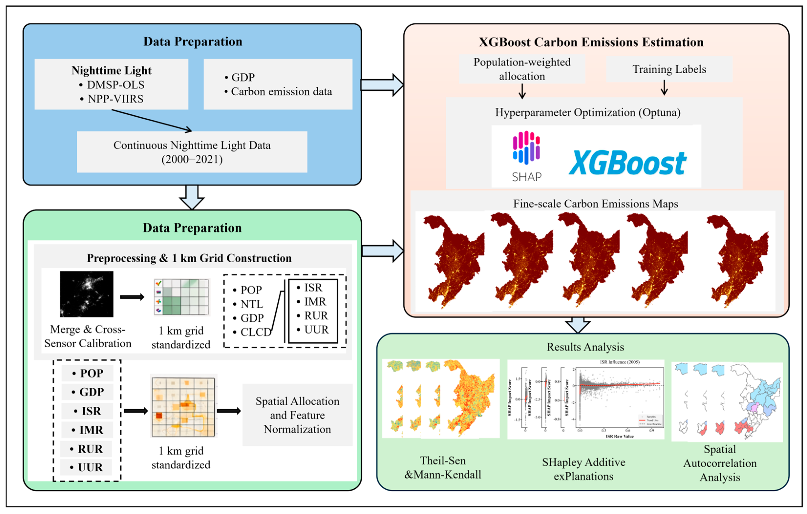
The methodology of this study is divided into three main parts. First, DMSP-OLS and NPP-VIIRS data are preprocessed and calibrated to construct a consistent time series covering the period from 2000 to 2021. Second, an XGBoost model is developed using POP, NTL, GDP, and land-use variables to estimate gridded carbon emissions at a spatial resolution of 1 km. Third, the spatiotemporal evolution and clustering characteristics of carbon emissions are analyzed at the grid, city, and county scales using trend analysis and spatial autocorrelation tests. In addition, the SHAP method is applied to identify the influences of key driving factors on carbon emissions across different development stages. The research technical framework is illustrated in Figure 2.

3.1. Preprocessing of Nighttime Light Data

DMSP-OLS data suffers from radiometric saturation (digital number range of 0–63) and limited interannual comparability. To address these limitations, this study employs the invariant region method to perform saturation correction and radiometric calibration. The DMSP-OLS satellites F14 (2002) and F16 (2005) are selected as reference years to establish the calibration relationships. When multiple products are available for the same year, they are fused to generate a representative annual stable light image [38,39]. To further mitigate the influence of light overflow, contemporaneously preprocessed NPP-VIIRS data are employed as a spatial mask to remove anomalous spillover pixels [40].

Monthly NPP-VIIRS data are prone to seasonal low-light omissions in high-latitude regions [40,41]. To construct a stable annual light series, only months with relatively stable illumination conditions (from September to March of the following year) are retained. Mean compositing is then applied to generate annual NTL images [42], and background noise is removed using masks derived from official annual VIIRS products.

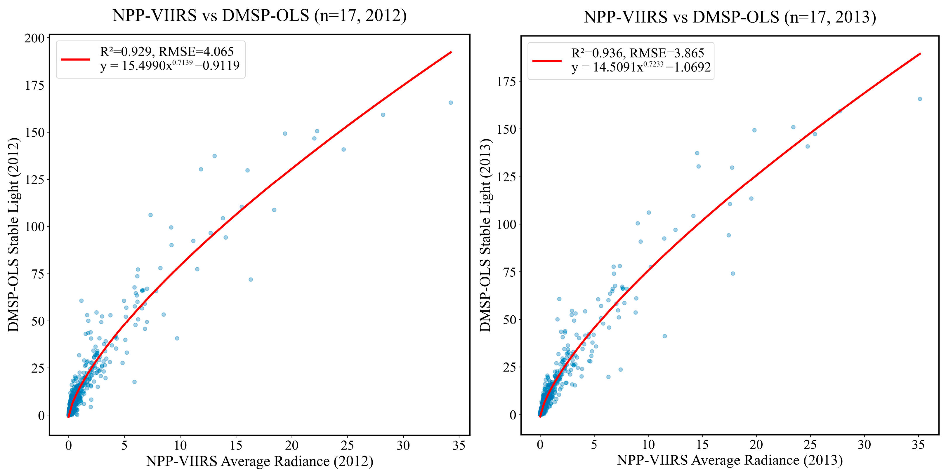
To achieve cross-sensor consistency between DMSP-OLS and NPP-VIIRS, a radiometric normalization model is established based on their overlapping years (2012 and 2013). First, the original 1 km pixels are spatially aggregated using an n × n moving window mean to generate resampled datasets at multiple aggregation scales. Subsequently, regression analyses are performed between contemporaneous NPP-VIIRS and DMSP-OLS data at each aggregation level, testing various functional forms, including linear, quadratic, exponential, and power-law models. The power-law calibration was selected after comparing linear, quadratic, exponential, and power-law functional forms. The power-law model achieved R² of 0.938 and 0.943 for 2012 and 2013 respectively, outperforming alternatives in capturing the nonlinear radiometric relationship between sensors. Resampling window sizes from n = 10 to n = 21 were tested. Performance improved steeply until n = 17 then plateaued, with marginal gains offset by computational cost and potential oversmoothing. The n = 17 configuration provided optimal balance between smoothing effectiveness and spatial detail preservation. The fitting results for 2013 are slightly superior to those for 2012. The final cross-sensor calibration model is presented in Equation (1), based on which a continuous NTL time series from 2000 to 2021 is constructed (Figure 3).

$$D{N}_{like}=14.5091\times D{N}_{NPP}^{0.7233}-1.0692$$

(1)

where DN_like denotes the brightness value of the DMSP-OLS like data after radiometric correction, and DN_NPP represents the brightness value derived from the NPP-VIIRS data.

3.2. Construction of the Carbon Emission Estimation Model

The spatialized estimation of CE consists of three main components: (1) construction of spatial grid units and feature extraction, (2) preparation of training labels, and (3) training and evaluation of the XGBoost model.

3.2.1. Spatial Grid Construction and Feature Extraction

A standardized 1 km × 1 km vector fishnet covering the three provinces of northeast China was constructed as the basic spatial analysis unit. To ensure spatial consistency in statistical analyses across multi-source raster datasets, a centroid-based allocation rule was applied for zonal statistics: a raster pixel was assigned to a target grid cell only when the geometric center of the original pixel fell within that grid. This approach minimizes boundary-induced biases and ensures comparability among datasets with different spatial characteristics.

Based on the grid units, seven feature variables were extracted or calculated, including NTL, POP, GDP, as well as four land-use structure indicators derived from the CLCD: impervious surfaces ratio (ISR), urban land-use ratio (UUR), rural land-use ratio (RUR), and industrial mining ratio (IMR). Together, these variables characterize variations in human activity intensity, economic scale, and land-use structure across space, providing a comprehensive feature set for carbon emission estimation and mechanism analysis. Variance inflation factors were calculated to assess predictor collinearity. VIF values ranged from 1.28 for RUR to 4.38 for GDP, all below the threshold of 10, indicating acceptable levels. The correlation matrix revealed moderate associations between GDP and NTL (r = 0.67) and between POP and GDP (r = 0.58), while land-use variables exhibited weaker intercorrelations (r < 0.45). XGBoost’s tree-based architecture naturally handles correlated predictors through recursive partitioning, and SHAP values remain interpretable given the moderate VIF range.

3.2.2. Preparation of Training Samples

To generate the labeled data required for model training, a spatial downscaling approach was employed. City-level carbon emission inventories provided by the China Emission Accounts and Datasets were combined with population data to redistribute emissions to the grid scale. Specifically, it was assumed that, within a given city, carbon emission intensity is positively correlated with population density. Accordingly, total city-level carbon emissions were allocated to 1 km grid cells using population-based weighting. The calculation procedure is expressed in Equation (2):

$$C{E}_{\mathit{grid}}=C{E}_{\mathit{city}}\times {\displaystyle \frac{{\mathit{POP}}_{\mathit{grid}}}{{\sum }_{i\in \mathit{city}}PO{P}_{\mathit{city}}}}$$

(2)

where CE_grid denotes the carbon emission of the target grid cell, CE_city represents the annual total carbon emissions of the city to which the grid cell belongs, POP_grid is the population within the grid cell, and POP_city denotes the total population of the corresponding city. This population-weighted allocation involves using POP both for spatial disaggregation and as a model predictor, which requires justification. Population density represents a causal driver of energy consumption across scales rather than merely a statistical artifact. The model incorporates independent covariates, including nighttime light, GDP, and land-use structure, which constrain emission patterns through different pathways, reducing reliance on population alone. The integration of multiple independent covariates (nighttime light, GDP, land-use structure) that constrain predictions through different pathways mitigates potential circularity effects. Limited external validation against available county-level inventories showed acceptable agreement, though systematic collection of finer-scale validation data remains a priority.

3.2.3. XGBoost Model Construction and Training

The Extreme Gradient Boosting (XGBoost) model is an efficient and flexible ensemble machine learning algorithm that iteratively constructs a series of weak learners (decision trees) [43]. XGBoost was selected based on demonstrated advantages in handling complex spatial data [43]. Compared to random forest, XGBoost incorporates second-order gradient information and explicit regularization, yielding superior accuracy in preliminary tests with R² improvements of 0.06–0.09. Relative to deep neural networks, XGBoost offers greater interpretability through its tree structure while requiring less hyperparameter tuning than support vector machines. The boosting framework naturally captures feature interactions and threshold effects that linear models cannot represent. At each iteration, subsequent trees are optimized based on the prediction errors of the previous ensemble, thereby progressively reducing bias and improving overall predictive accuracy. The objective function of XGBoost is formulated under the principle of structural risk minimization, simultaneously accounting for empirical loss and model complexity during each boosting step. This design enables the resulting model to achieve strong generalization performance while retaining a high degree of interpretability [44,45].

The model prediction is expressed as the additive output of all individual trees, and the final estimated value can be represented as shown in Equation (3).

$${\widehat{y}}_i^{\left(t\right)}={\sum }_{k=1}^t{f}_k\left(x_i\right)$$

(3)

where denotes the predicted value of sample i after the t-th iteration, and f_k(x_i) represents the base learner (weak model) constructed in the k-th boosting round.

The objective function at the t-th iteration is defined as:

$$\mathit{obj}\left(\theta \right)={\sum }_i^{n}L(y_i,{\widehat{y}}_i)+{\sum }_{k=1}^K\mathrm{\Omega }(f_k)$$

(4)

$$\Omega (f_k)=\gamma T+{\displaystyle \frac{1}{2}}\lambda {\sum }_{j=1}^T{\omega }_j^2$$

(5)

where denotes the loss function, and Ω(fk) represents the regularization term. Here, T is the number of leaf nodes in the tree, ω_j denotes the score assigned to the j-th leaf node, and γ and β are hyperparameters that control model complexity. The optimized hyperparameter settings of the model are summarized in

Table 3. Optimized hyperparameters obtained using the Optuna framework.

Category	Parameter	Value	Description
Data partitioning	Train/Test split	80%/20%	Training subset used for model fitting; testing subset reserved for independent evaluation
Model complexity	n_estimators	100	Number of base learners (decision trees), corresponding to the number of boosting iterations
Tree structure	Max_depth	5	Maximum depth of individual trees, controlling model complexity and mitigating overfitting
Split regularization	gamma	0.1	Minimum loss reduction required to make a further partition, enforcing conservative tree splitting
Reproducibility	Random state	42	Fixed random seed to ensure reproducible data partitioning and model training

.

Model performance was assessed using both random holdout and spatial cross-validation. The standard approach employed 80/20 train-test split with random city sampling. However, given strong spatial autocorrelation (Global Moran’s I exceeding 0.64), random splitting may yield optimistic estimates due to spatial proximity between training and testing samples. Spatial cross-validation was therefore implemented by partitioning the study region into five contiguous blocks: southern Liaoning, northern Liaoning, Jilin Province, western Heilongjiang, and eastern Heilongjiang. In each fold, one block served as the test set while remaining blocks formed the training set, ensuring geographic separation. This leave-region-out approach provides more conservative assessment of model transferability. Prediction uncertainty was quantified through bootstrap resampling with 100 iterations. In each iteration, cities were randomly sampled with replacement and the model was retrained. The 2.5th and 97.5th percentiles of bootstrap distributions provided 95% confidence intervals for performance metrics and SHAP values, accounting for sampling variability and model instability.

3.3. Quantifying Feature Contributions and Dependence Relationships of XGBoost Outputs Using SHAP

To elucidate the interpretability of model outputs, this study employs the SHapley Additive exPlanations (SHAP) approach to perform post hoc interpretation of the XGBoost model [46]. SHAP is grounded in Shapley values from cooperative game theory and decomposes the prediction of an individual sample into the additive contributions of each feature, satisfying the properties of consistency and additivity [47].

For a trained XGBoost model, the predicted output for sample i can be expressed as the sum of the baseline prediction and the SHAP contributions of individual features:

$${\widehat{y}}_i={\mathsf{\varphi }}_0+{\sum }_{j=1}^M{\mathsf{\varphi }}_{i,j}$$

(6)

where ${\varphi }_0$ denotes the expected model output over all training samples, representing the global baseline value. The term ${\varphi }_{I,\mathrm{j}}$ represents the SHAP contribution of feature j to the prediction of sample i A positive value of ${\varphi }_{I,\mathrm{j}}$ indicates that the feature increases the predicted value, whereas a negative value indicates a suppressing effect.

3.4. Theil–Sen Slope Estimation

The Theil–Sen slope estimator is a nonparametric statistical method widely used for trend detection in time series. In this study, the Theil–Sen approach was employed to calculate the slopes between all pairwise observations in the CE time series. The median of these pairwise slopes was then adopted as a robust indicator of the overall trend in CE dynamics, effectively reducing the influence of outliers and non-normal data distributions. The computational procedure is described as follows:

$$\beta =\mathit{Median}\left({\displaystyle \frac{C{E}_j-C{E}_i}{j-i}}\right),j>i$$

(7)

where CE_j and CE_j denote the carbon emissions in years j and i, respectively, and β represents the median of all pairwise slopes. When β > 0, carbon emissions exhibit an increasing trend, whereas β < 0 indicates a decreasing trend in carbon emissions [48].

3.5. Mann–Kendall Trend Test

The Mann–Kendall (MK) test is a nonparametric statistical method that is commonly used as a complement to the Theil–Sen slope estimator to assess the statistical significance of monotonic trends in time series data [49]. Owing to its minimal distributional assumptions, the MK test is well-suited for analyzing environmental and socioeconomic time series characterized by non-normality, missing values, or outliers.

In this study, the Mann–Kendall test is applied to evaluate the significance of temporal trends in CE. The test statistic is computed as follows:

$$S={\sum }_{i=1}^{n-1}{\sum }_{j=i+1}^n\mathit{sign}(C{E}_j-C{E}_i)$$

(8)

$$\mathit{sign}(C{E}_j-C{E}_i)=\left\{\begin{array}{ll}1& C{E}_j-C{E}_i>0\\ 0& C{E}_j-C{E}_i=0\\ -1& C{E}_j-C{E}_i<0\end{array}\right.$$

(9)

The variance can be calculated using the following method:

$$\mathit{var}(s)={\displaystyle \frac{n(n-1)(2n+5)}{18}}$$

(10)

$$Z=\left\{\begin{array}{ll} {\displaystyle \frac{S-1}{\sqrt{\mathit{var}(S)}}}& S>0\\ 0& S=0\\ {\displaystyle \frac{S+1}{ \sqrt{\mathit{var}(S)}}}& S<0\end{array}\right.$$

(11)

where S denotes the test statistic, n is the length of the time series, sign(•) represents the sign function, and Z is the standardized test statistic. At the significance level α = 0.05, if |Z| > Z_1−α/2, the null hypothesis of no trend is rejected, indicating the presence of a statistically significant trend in the series. The direction of the trend is determined by the sign of S: S > 0 indicates an increasing trend, whereas S < 0 indicates a decreasing trend.

3.6. Spatial Autocorrelation Analysis

To reveal the spatial dependence and heterogeneity of CE in northeast China, spatial autocorrelation analysis is employed in this study. First, the Global Moran’s I statistic is used to evaluate whether CE exhibits significant spatial clustering or dispersion across the entire study region. The corresponding calculation is expressed as follows:

$$I={\displaystyle \frac{n{\sum }_{i=1}^n{\sum }_{j=1}^n{W}_{\mathit{ij}}(X_i-\overline{X})(X_j-\overline{X})}{{\sum }_{i=1}^n{\sum }_{j=1}^n{W}_{\mathit{ij}}{\sum }_{i=1}^n(X_i-\overline{X}{)}^2}}$$

(12)

where n denotes the total number of spatial units, X_i and X_j represent the carbon emissions of spatial units i and j, respectively, and $\overline{X}$ is the mean value of carbon emissions across all units. The term W_ij denotes the spatial weight matrix describing the neighborhood relationship between units i and j. The value of Moran’s I ranges from −1 to 1, with values closer to 1 indicating stronger positive spatial autocorrelation, whereas values closer to −1 indicate stronger negative spatial autocorrelation.

Local spatial autocorrelation, measured using Anselin’s Local Moran’s I, is examined through Local Indicators of Spatial Association (LISA) to assess the degree of clustering between a focal spatial unit and its neighboring units. The statistic is computed as follows:

$$I_i={\displaystyle \frac{n(X_i-\overline{X}){\sum }_{j=1}^n{W}_{\mathit{ij}}(X_j-\overline{X})}{{\sum }_{i=1}^n(X_i-\overline{X}{)}^2}}$$

(13)

Based on the Local Moran’s I values and their corresponding significance levels, each spatial unit can be classified into five categories: High–High (HH), Low–Low (LL), High–Low (HL), Low–High (LH), and statistically non-significant areas. This classification facilitates the precise identification of carbon emission hotspots, cold spots, and spatial heterogeneity patterns.

4. Results

4.1. Spatiotemporal Dynamics of Carbon Emissions in Northeast China

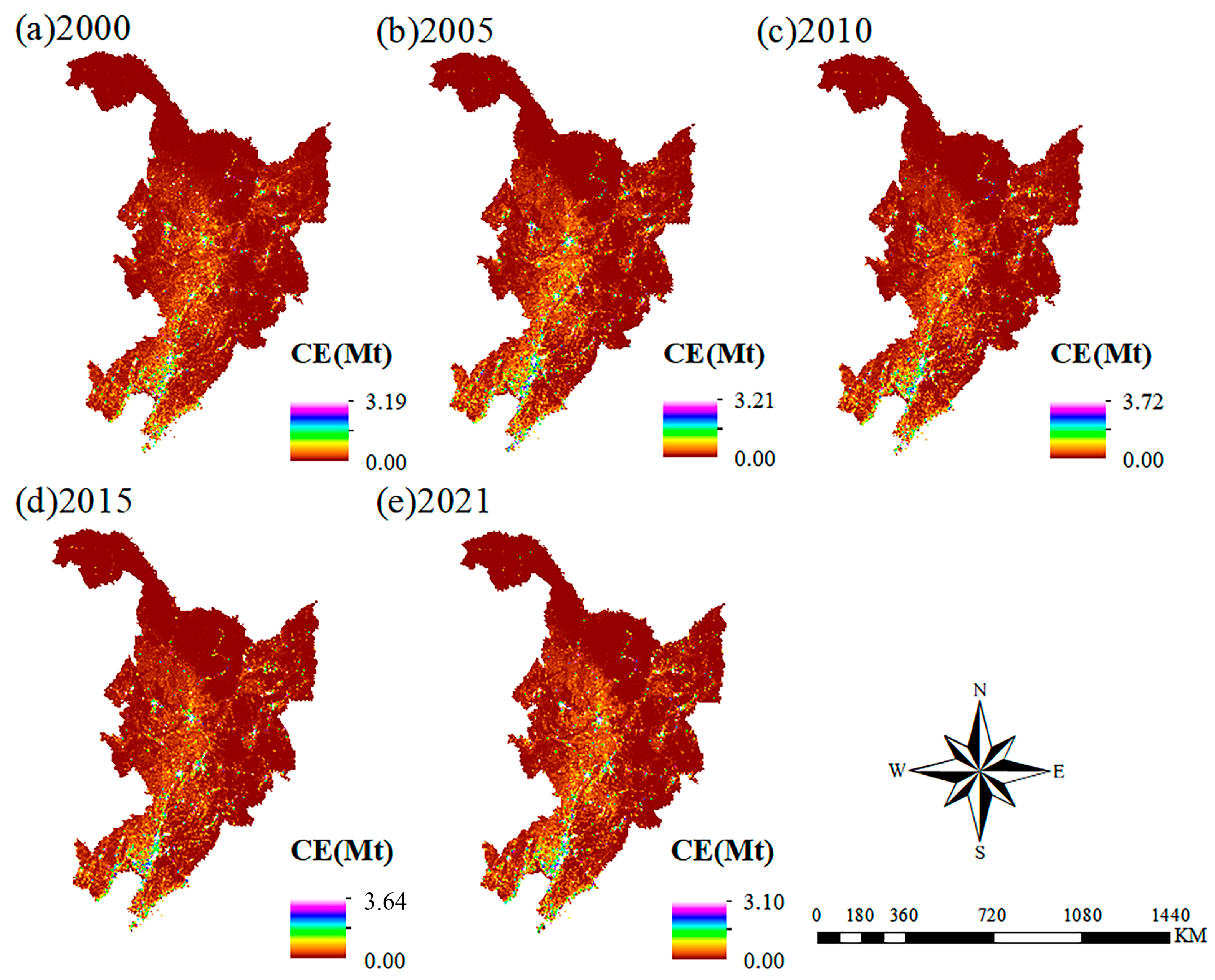
Figure 4 illustrates the spatial evolution of CE at the 1 km × 1 km grid scale in northeast China from 2000 to 2021. Overall, the region exhibits a pronounced spatial differentiation pattern characterized by “higher emissions in the south and lower emissions in the north,” accompanied by distinct point–axis agglomeration features.

From a spatial distribution perspective, high-intensity emission areas (2.5 Mt/grid) have remained persistently concentrated in the central and southern urban belt of Liaoning Province, with the Shenyang–Anshan–Dalian axis being particularly prominent. In 2021, the maximum grid-level CE in this corridor reached 3.10 Mt/grid, showing only a slight decline compared with 2000 (3.19 Mt/grid) while still maintaining a high emission level. Northern and eastern Heilongjiang Province generally exhibit relatively low emission intensities; however, a secondary high-value axis formed by Harbin–Qiqihar–Daqing is clearly identifiable. In Jilin Province, the spatial pattern is characterized by a monocentric structure centered on the Changchun–Jilin urban core, displaying a radiation-like expansion toward surrounding areas.

In terms of temporal evolution, the period from 2000 to 2010 represents a phase of rapid carbon emission expansion. A comparison between Figure 4a,c shows that the spatial extent of emitting grids expanded markedly along the peripheries of major urban agglomerations. In southern Liaoning, high-emission areas evolved from scattered point distributions in 2000 into contiguous patches by 2010. Moreover, high-value zones in central Liaoning (Shenyang–Fushun–Benxi) and southern Liaoning (Yingkou–Dalian) gradually merged, forming a continuous high-emission belt. After 2015 (Figure 4d,e), regional CE entered a phase of fluctuating adjustment, with the spatial pattern exhibiting a dual characteristic of “peripheral contraction and internal intensification.”

At the provincial scale, notable differences are observed in total CE. Heilongjiang’s total CE increased from 209.87 Mt to 344.01 Mt, exhibiting relatively steady growth over the study period. Jilin recorded the lowest absolute emissions among the three provinces, but its total CE rose from 139.14 Mt to 267.33 Mt, corresponding to a growth rate of nearly 92%, the fastest among the three provinces. Liaoning, as the traditional heavy industrial core of northeast China, experienced an increase in CE from 287.20 Mt to 519.72 Mt, ranking first in both absolute growth and total emission scale. Normalized intensity metrics reveal divergent trajectories. Liaoning’s per capita emissions increased from 6.53 to 12.20 tCO₂/person, consistently exceeding the national average. Emission intensity per GDP decreased from 0.45 to 0.19 tCO₂/billion CNY, indicating decoupling yet remaining above the national level. Jilin exhibited the steepest intensity reduction from 0.48 to 0.20 tCO₂/billion CNY, partially offsetting high absolute growth. Heilongjiang maintained moderate per capita emissions (5.52 to 10.80 tCO₂/person) with intensity decreasing from 0.66 to 0.23 tCO₂/billion CNY, reflecting persistent reliance on extractive industries.

4.1.1. Growth Characteristics of Carbon Emissions at the City and County Levels

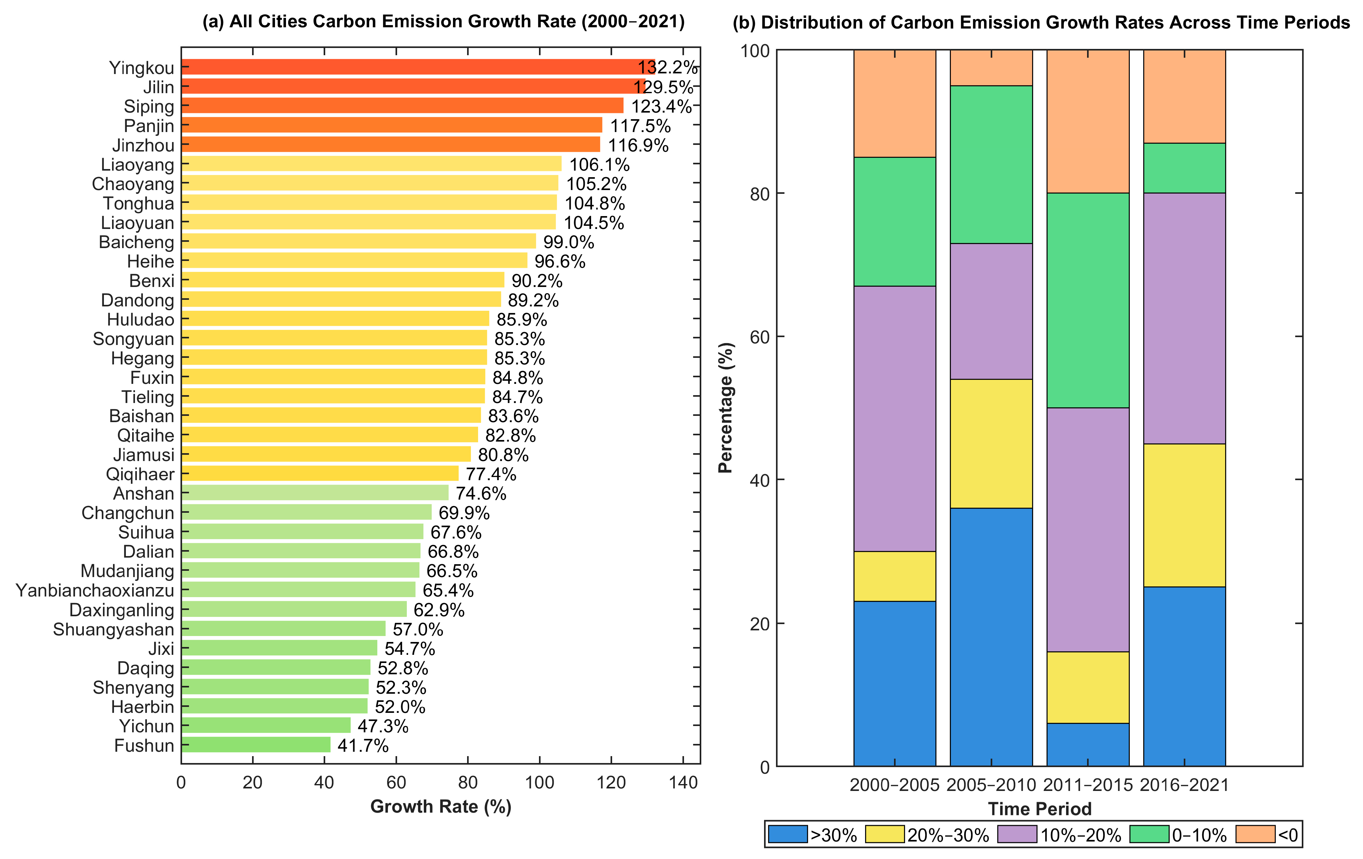
Figure 5a illustrates changes in city-level carbon emission growth rates from 2001 to 2021. Overall, CE exhibit a predominantly positive growth trend, with particularly pronounced increases observed in several resource-based and old industrial cities. Cities such as Yingkou, Jilin, Siping, Panjin, Jinzhou, Liaoyang, Chaoyang, Tonghua, and Liaoyuan all recorded growth rates exceeding 100%, with most of these high-growth cities concentrated in southern Liaoning Province.

The stage-wise analysis shown in Figure 5b further reveals distinct temporal dynamics. During the periods 2000–2005 and 2005–2010, the proportion of cities falling within the high-growth interval (20%) reached 30% and 54%, respectively, indicating a phase of rapid and widespread emission expansion. In contrast, during 2011–2015, the share of cities in the high-growth category declined sharply, while the proportion of cities with growth rates below 10% increased to approximately 50%, reflecting a pronounced deceleration in emission growth. In the most recent period, 2016–2021, carbon emission growth became increasingly differentiated: cities with moderate growth rates dominated, alongside a noticeable rise in the proportion of cities experiencing negative growth.

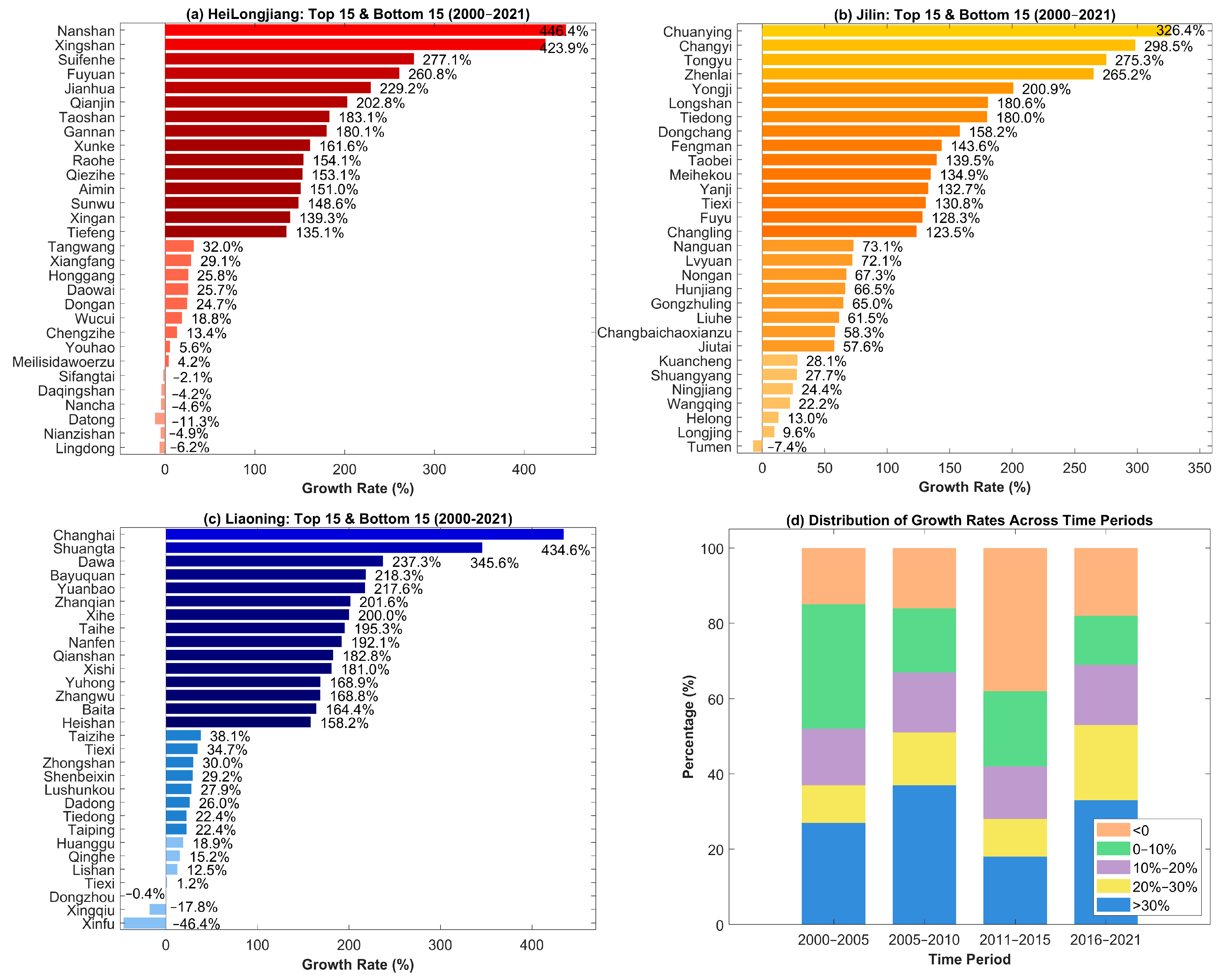
Given that the number of county-level units reaches 282, only the 15 counties with the highest and lowest CE growth rates in each province are presented to highlight extreme contrasts. As shown in Figure 6a, county-level CE growth in Heilongjiang Province exhibits a highly dispersed and strongly polarized “dual-tail” structure. On the one hand, a small number of counties form a pronounced high-growth tail, including Nanshan (446%), Xingshan (424%), Suifenhe (277%), and Fuyuan (261%). On the other hand, several counties experienced substantial emission contraction, such as Lingdong (−47%), Nianzishan (−25%), and Datong (−11%).

In contrast, Jilin Province displays generally higher county-level CE growth rates (Figure 6b), with emissions remaining predominantly positive and negative growth being rare. Growth magnitudes are mainly concentrated in the medium-to-high range. Counties such as Chuanying (326%), Changyi (299%), Tongyu (275%), and Zhenlai (265%) exhibit leap-type growth, whereas Tumen (−7%) and Longjing (9.6%) represent the few counties with stagnant or declining emissions.

Liaoning Province is characterized by a relatively high proportion of counties with rapid CE growth (Figure 6c), while only three counties fall into the negative growth category. Changhai (435%), Shuangta (346%), Dawa (237%), Bayuquan (218%), and Yuanbao (218%) show the fastest growth, whereas Xinfu (−46.7%) and Xinqiu (−17.8%) experienced notable declines.

The stage-wise distribution shown in Figure 6d further reveals the temporal evolution of county-level CE growth structures. During 2000–2005, the growth pattern was relatively dispersed across counties. Between 2005 and 2010, the share of high-growth counties increased markedly, indicating an accelerated phase of regional expansion. In 2011–2015, high-growth shares declined, accompanied by simultaneous increases in low-growth and negative-growth counties. During 2016–2021, the proportion of high-growth counties rebounded, and the growth structure was reorganized, suggesting that some counties entered a phase of recovery-oriented growth.

4.1.2. Growth Trend Characteristics at the Grid Scale

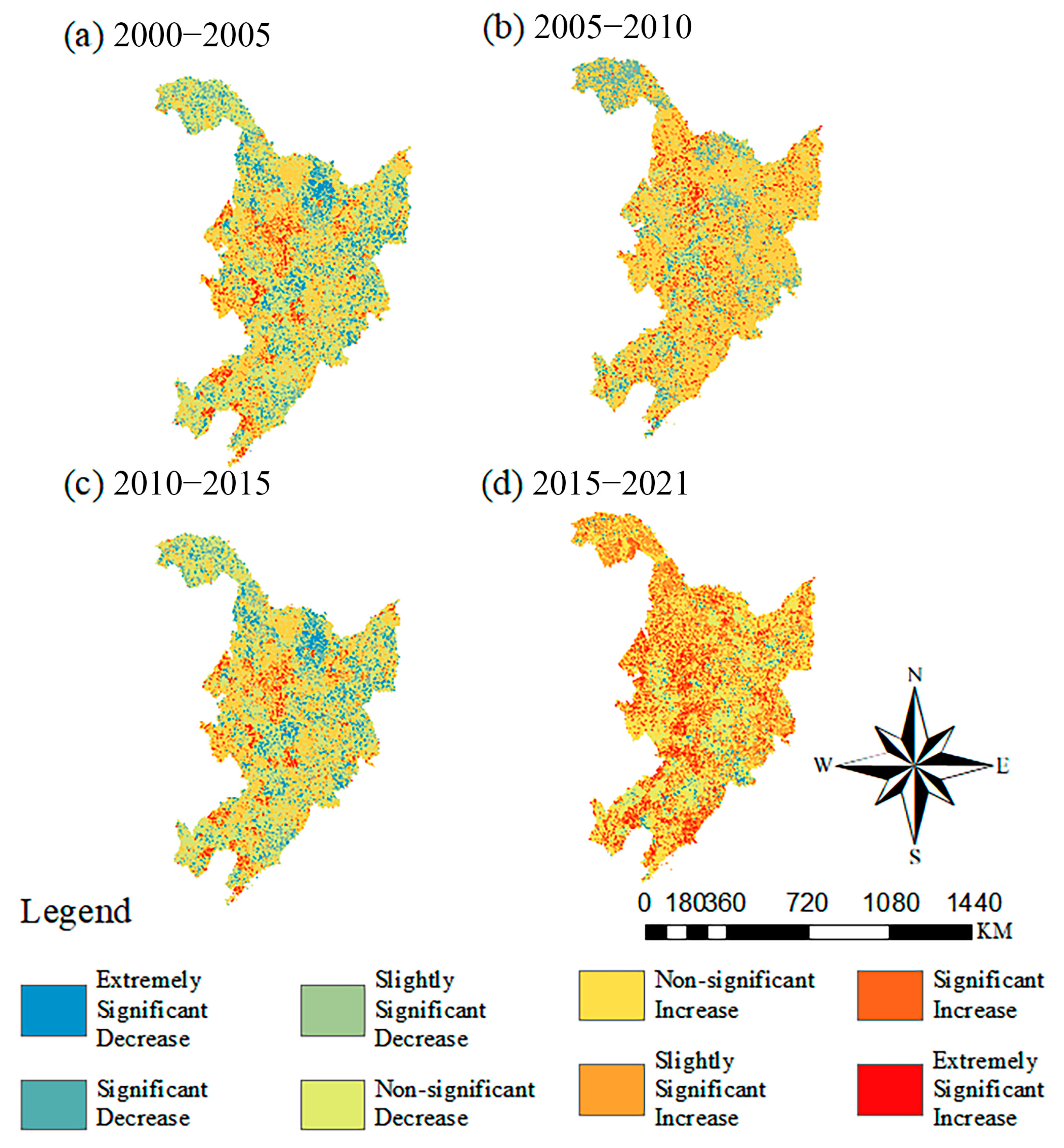
Figure 7 illustrates the grid-level trends of CE changes across northeast China during different sub-periods from 2000 to 2021. Overall, CE dynamics exhibit pronounced stage-dependent differences, alongside an evolutionary shift from spatially fragmented patterns toward more continuous configurations. During the 2000–2005 period (Figure 7a), the spatial pattern of CE trends is highly fragmented, with pixels exhibiting increasing and decreasing tendencies interwoven across the region, and no large-scale contiguous clusters yet formed. In the 2005–2010 period (Figure 7b), increasing trends clearly dominate spatially, with extensive areas showing slight to significant growth, while the spatial extent of decreasing trends contracts markedly and becomes confined to localized areas. During 2010–2015 (Figure 7c), increasing and decreasing trends coexist across the region, accompanied by a rising proportion of pixels exhibiting non-significant changes, leading to a renewed dispersal of the spatial pattern. In contrast, during the 2015–2021 period (Figure 7d), increasing trends overwhelmingly dominate and form large, contiguous spatial zones, indicating a phase characterized by strong spatial continuity in emission growth.

4.2. Spatial Clustering Patterns of Carbon Emissions

Table 4. Changes in Moran’s I from 2001 to 2021.

Year	City Level CE			County Level CE
	Moran_I	p_Value	z_Score	Moran_I	p_Value	z_Score
2000	0.642	0.000	6.063	0.329	0.000	8.645
2001	0.647	0.000	6.100	0.307	0.000	8.058
2002	0.637	0.000	6.012	0.313	0.000	8.228
2003	0.661	0.000	6.229	0.301	0.000	7.920
2004	0.659	0.000	6.218	0.296	0.000	7.783
2005	0.660	0.000	6.226	0.295	0.000	7.758
2006	0.651	0.000	6.139	0.321	0.000	8.425
2007	0.647	0.000	6.107	0.332	0.000	8.724
2008	0.695	0.000	6.540	0.349	0.000	9.167
2009	0.694	0.000	6.529	0.349	0.000	9.164
2010	0.687	0.000	6.471	0.339	0.000	8.909
2011	0.694	0.000	6.528	0.346	0.000	9.070
2012	0.687	0.000	6.465	0.303	0.000	7.971
2013	0.666	0.000	6.275	0.292	0.000	7.668
2014	0.674	0.000	6.352	0.301	0.000	7.916
2015	0.673	0.000	6.336	0.302	0.000	7.934
2016	0.678	0.000	6.385	0.304	0.000	8.001
2017	0.688	0.000	6.474	0.331	0.000	8.681
2018	0.695	0.000	6.536	0.326	0.000	8.574
2019	0.698	0.000	6.563	0.331	0.000	8.701
2020	0.697	0.000	6.561	0.326	0.000	8.556
2021	0.700	0.000	6.586	0.310	0.000	8.153

reports the global Moran’s I statistics at both the city and county levels over the study period. For all years, Moran’s I values are positive and pass the 0.1% significance test, indicating statistically significant positive spatial autocorrelation at the 95% confidence level. These results demonstrate a pronounced spatial clustering of CE, particularly at the city scale.

At the city level, Moran’s I increases from 0.642 in 2000 to 0.700 in 2021, suggesting a continuous strengthening of spatial dependence between high-emission and low-emission city clusters over time. In contrast, county-level Moran’s I values range between 0.292 and 0.349, reflecting substantially weaker clustering intensity than that observed at the city level. This indicates that CE distributions at finer spatial scales are more dispersed and exhibit stronger local heterogeneity.

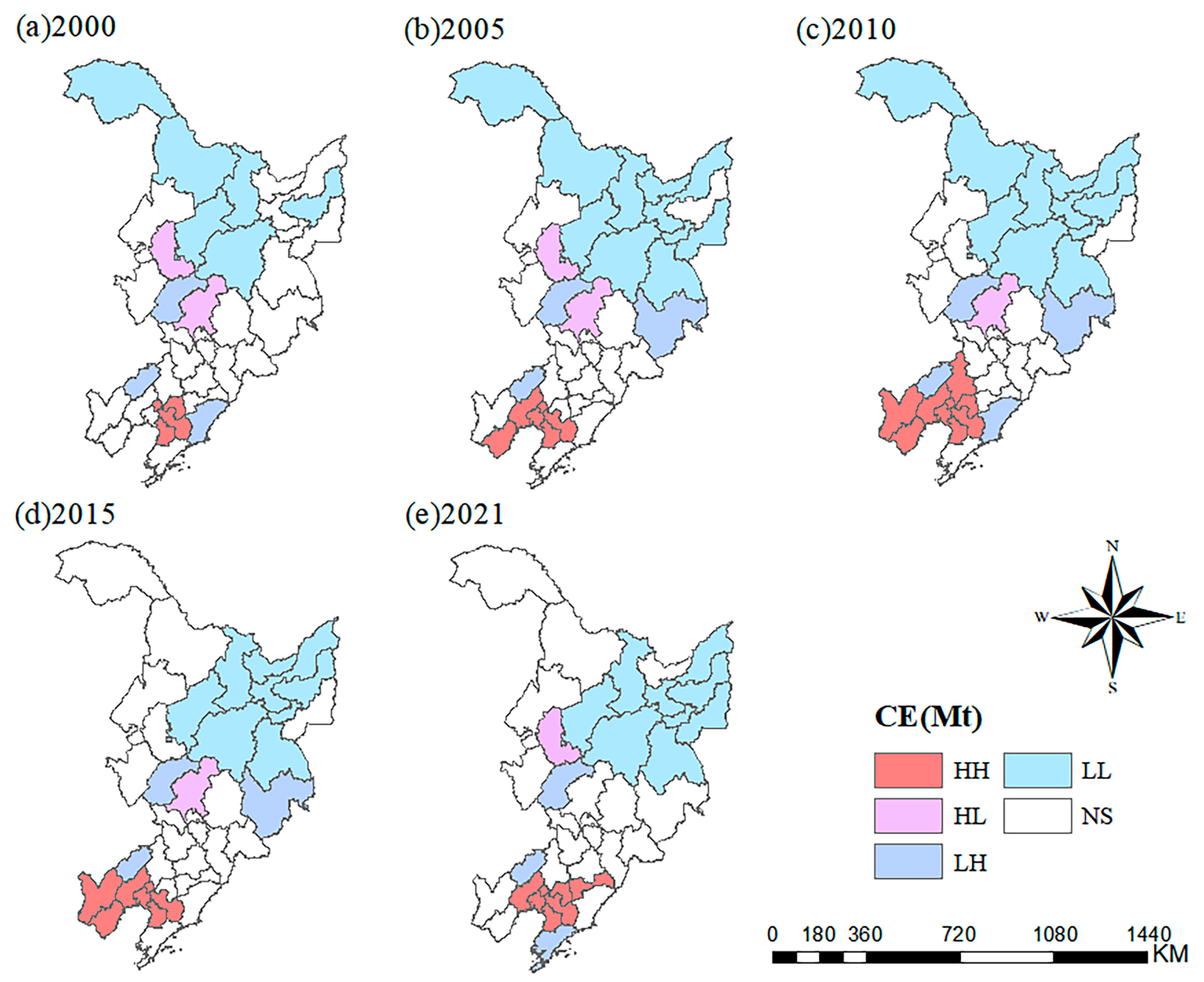
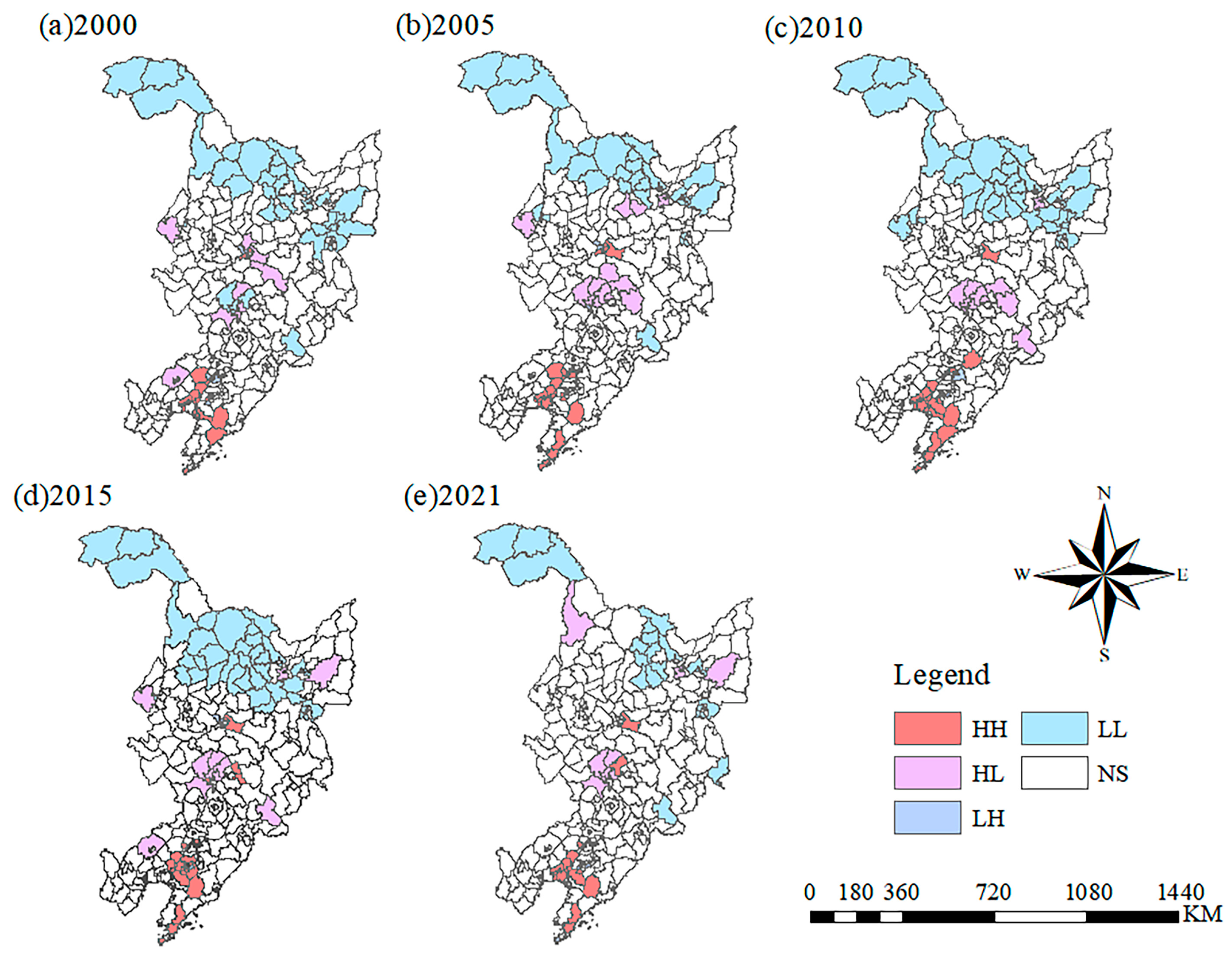
The city-level LISA clustering results (Figure 8) reveal pronounced spatial agglomeration patterns and strong path dependence in CE. Overall, HH clusters have remained persistently concentrated in southern Liaoning Province, centered on the Anshan–Yingkou–Dalian corridor, forming a sustained high-emission “hotspot” region. These cities consistently exhibit significant HH clustering across all five study years, indicating the formation of a stable spatial association network among high-emission cities. In contrast, LL clusters are mainly distributed in northern and eastern Heilongjiang Province, represented by cities such as Heihe, Yichun, Jiamusi, and Hegang, forming a low-emission belt with strong spatial continuity. The spatial connectivity of LL clusters reached its maximum around 2010 and subsequently showed a slight contraction.

During the period 2000–2010, high-value clustering in southern Liaoning expanded from a limited number of cities in 2000 into a contiguous and stable high-emission agglomeration belt. Over the same period, LL clusters extended southeastward from the northern border areas of Heilongjiang, gradually encompassing several resource-based and resource-depleted cities. After 2015, both HH and LL clusters experienced varying degrees of contraction, and the overall spatial configuration tended to stabilize. In comparison, heterogeneous clustering types (HL and LH) are relatively scattered at the city scale and are primarily located along the peripheries of high- and low-value clusters, exerting limited spatial influence.

The county-level LISA clustering results (Figure 9) further reveal scale-dependent differences and pronounced micro-level heterogeneity in the spatial pattern of CE. Compared with the city scale, county-level CE also exhibits clear HH and LL clustering characteristics; however, the spatial distribution is more fragmented, clustering intensity is relatively weaker, boundary structures are more complex, and the number of heterogeneous clusters (HL and LH) increases markedly.

HH clusters are mainly distributed along the peripheries of city-level hotspots and within contiguous industrial concentration areas, displaying a multicentric and cluster-based spatial configuration. The number of HH-clustered counties in southern Liaoning peaked around 2010, reaching approximately 18 counties. Typical HH counties include Tiexi District and Lishan District in Anshan, Dashiqiao in Yingkou, and Zhuanghe in Dalian. In contrast, LL clusters are widely distributed across northern and eastern Heilongjiang as well as eastern Jilin, forming spatially continuous low-emission zones. Although their overall continuity remains strong, internal heterogeneity within LL clusters is notably higher at the county scale than at the city scale.

Heterogeneous clustering types (HL and LH) also become substantially more prominent at the county level, primarily concentrated in urban–rural transition zones and areas undergoing industrial restructuring. These patterns highlight the increasing importance of local socioeconomic conditions and land-use transitions in shaping fine-scale carbon emission dynamics.

4.3. Interactions Among Driving Factors and Spatiotemporal Evolution Mechanisms

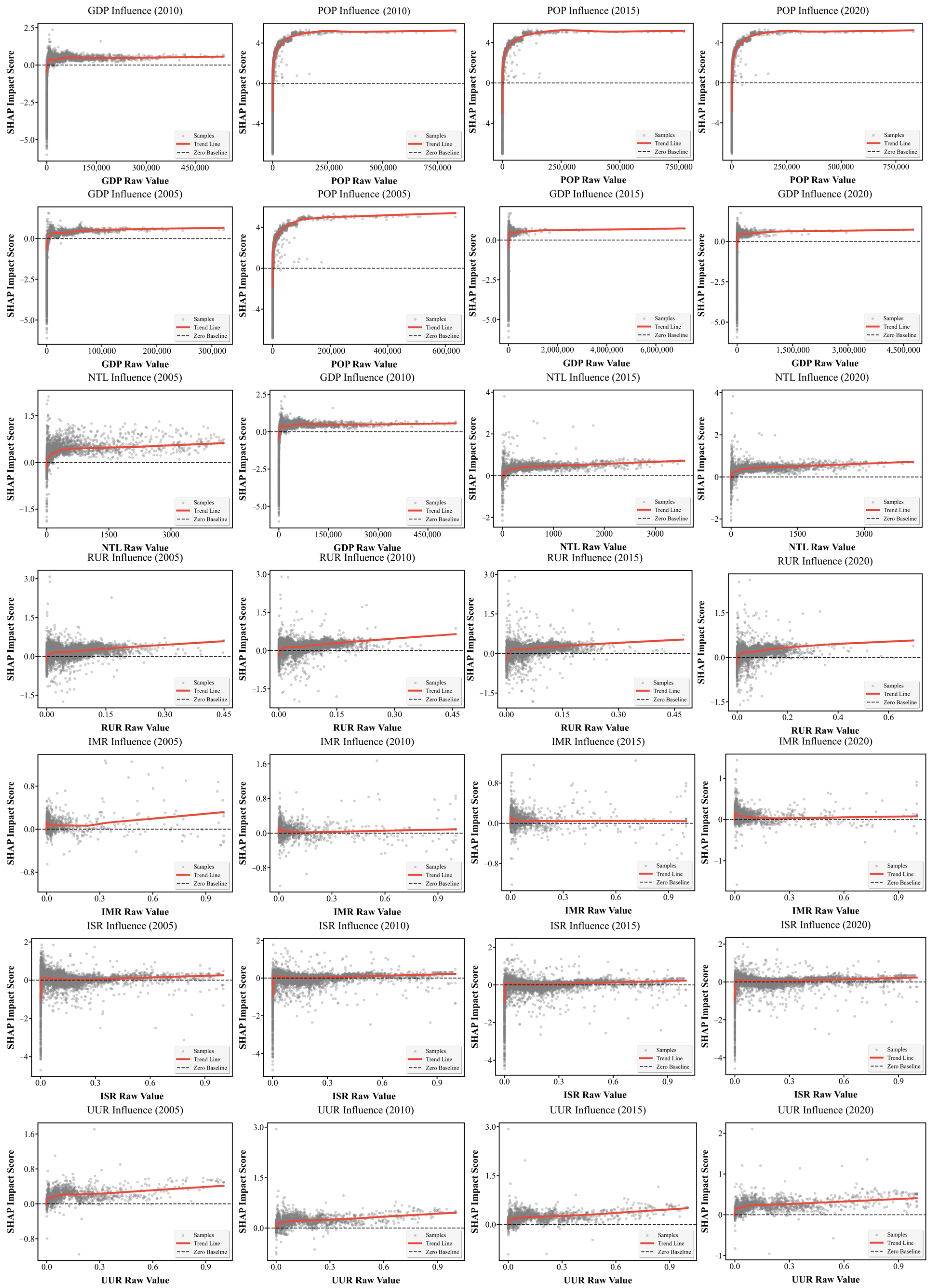
Based on SHAP dependence plots derived from the XGBoost models for 2005–2020 (Figure 10), this study reveals the spatiotemporal evolution and nonlinear response patterns of CE driving mechanisms in northeast China.

The influence of POP on CE exhibits a pronounced S-shaped nonlinear pattern over the study period, capturing a complete transition from strong driving effects to saturation. In 2005, SHAP values for POP increase rapidly within low- to medium-population ranges before approaching saturation. Over time, this saturation threshold shifts progressively toward lower population levels, indicating a gradual weakening of the marginal contribution of population growth to CE. Meanwhile, the range of negative SHAP values in low-population areas narrows year by year, suggesting that even in sparsely populated regions, baseline energy demand constitutes a non-negligible emission foundation.

The effect of GDP on CE undergoes a qualitative transition from strong linear association to weak positive persistence. During 2005–2010, GDP exerts a pronounced positive influence on CE within lower value ranges. After 2015, however, although GDP continues to expand in absolute terms, the SHAP dependence curve flattens rapidly beyond relatively low thresholds, and by 2020 approaches an almost fully saturated state. This pattern indicates the gradual emergence of decoupling between economic growth and CE.

The contribution of NTL to CE evolves from logarithmic growth in 2005 toward near saturation by 2020. During 2005–2010, NTL strongly promotes CE within low-intensity ranges. By 2020, this effect stabilizes beyond relatively low thresholds and remains strongly positive only in a limited number of high-intensity urban cores, suggesting that the marginal impact of urban activity intensity on CE is converging.

The proportions of ISR and IMR display generally weak associations with CE. Across all years, the ISR dependence curves remain close to the zero baseline, with increasing dispersion of SHAP values over time, indicating limited explanatory power when considered in isolation. The positive effect of IMR weakens continuously from 2005 to 2020 and nearly disappears by 2020, reflecting a substantial decline in the marginal contribution of industrial land expansion to emission growth.

The RUR and UUR maintain relatively stable positive effects on CE, though their modes of influence change over time. RUR exhibits a consistently moderate linear positive relationship across all years, implying a long-term cumulative effect of energy consumption associated with dispersed land-use patterns. In contrast, UUR shifts from rapid nonlinear growth during 2005–2010 to a more stable linear response during 2015–2020, indicating a stabilization of its impact on CE.

Synthesizing the SHAP dependence results for 2005–2020, three prominent characteristics of CE driving mechanisms in northeast China can be identified. First, the importance structure of driving factors undergoes a clear transformation: dominance by population and economic factors during 2005–2010 gives way to the joint influence of spatial structure and land-use configuration during 2015–2020, accompanied by marked saturation and weakening of the marginal effects of POP and GDP. Second, nonlinear characteristics deepen further by 2020, with nearly all driving factors exhibiting saturation or threshold effects, indicating well-defined bounds to their influence on CE. Third, the role of factor interactions becomes increasingly salient. The growing dispersion of SHAP values for variables such as ISR and IMR suggests that no single factor can adequately explain CE variation. Moreover, the widespread scatter observed across all SHAP dependence plots reflects the high degree of heterogeneity in resource endowments, industrial structures, and energy supply systems across northeast China.

5. Discussion

5.1. Model Performance Evaluation and Spatiotemporal Applicability

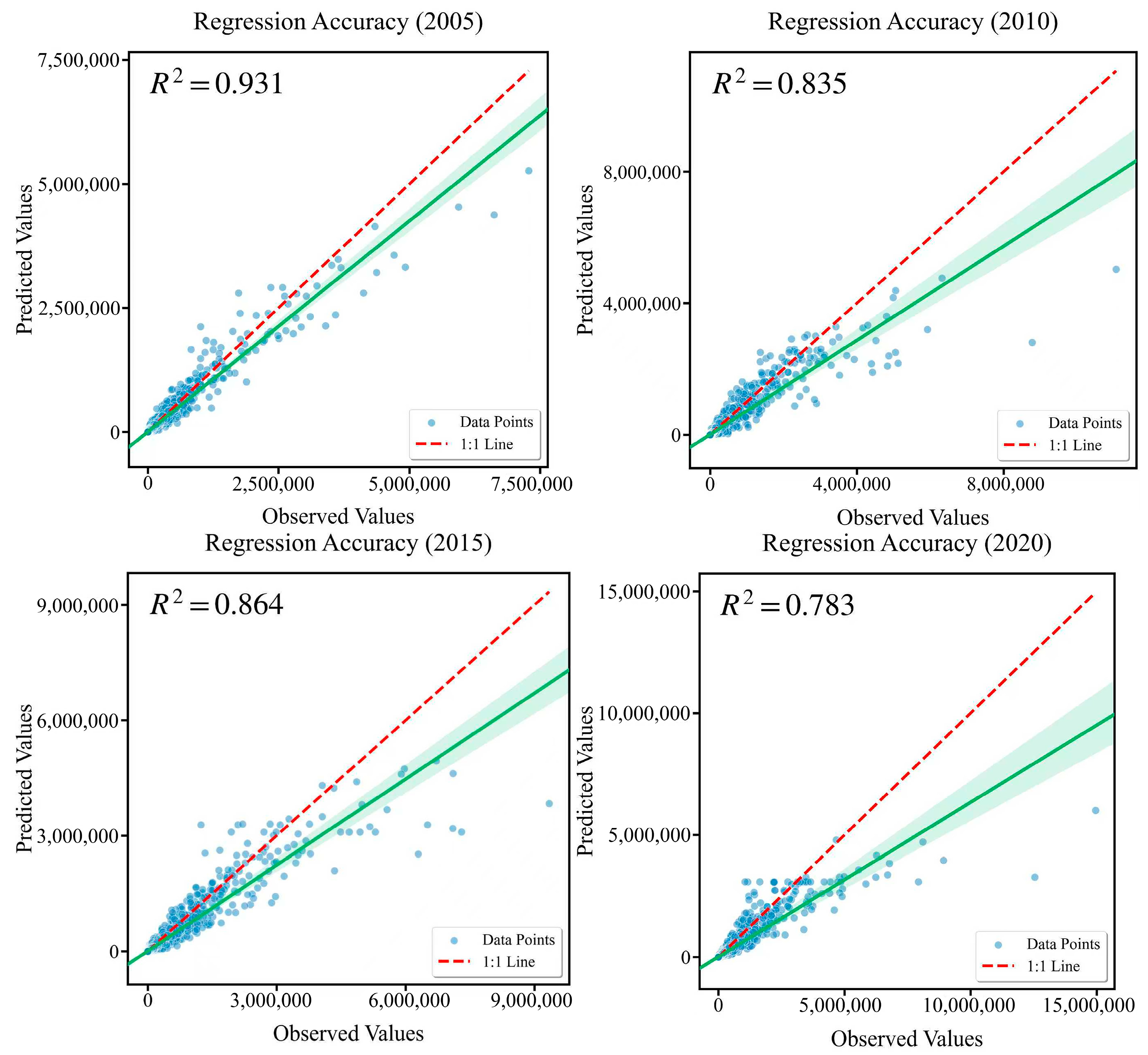
The XGBoost-based spatialization model for carbon emissions exhibits good predictive performance at the regional scale (Figure 11). Across the four benchmark years from 2005 to 2020, R² ranges from 0.783 (95% CI: 0.765–0.801) to 0.931 (95% CI: 0.913–0.947) under random split, while spatial cross-validation yields 0.731 (95% CI: 0.712–0.748) to 0.881 (95% CI: 0.865–0.895) (

Table 5. Performance comparison between random split and spatial cross-validation.

Year	Random R2 (95% CI)	Spatial CV R2 (95% CI)	Random MAE (Mt)	Spatial MAE (Mt)
2005	0.931 (0.913–0.947)	0.881 (0.865–0.895)	0.007	0.009
2010	0.876 (0.859–0.892)	0.828 (0.811–0.843)	0.012	0.015
2015	0.815 (0.798–0.831)	0.767 (0.749–0.783)	0.015	0.019
2020	0.783 (0.765–0.801)	0.731 (0.712–0.748)	0.016	0.020

). Mean absolute error remains stable between 0.007 Mt (95% CI: 0.006–0.008) and 0.016 Mt (95% CI: 0.014–0.018), while RMSE varies from 0.059 Mt (95% CI: 0.053–0.065) to 0.130 Mt (95% CI: 0.119–0.142). The moderate performance gap between random and spatial validation (ΔR² = 0.04–0.06) reflects prediction challenges in geographically distant regions but confirms adequate transferability.

The temporal variation in R² shows a pattern of decline, partial recovery, and subsequent decrease, reflecting the stage-dependent evolution of carbon emission driving mechanisms. In 2005, the relationships between carbon emissions and key drivers such as population and GDP were relatively stable and exhibited stronger linear characteristics, which facilitated effective model fitting. After 2010, with ongoing industrial restructuring, improvements in energy efficiency, and the implementation of energy conservation and emission reduction policies, the formation mechanisms of carbon emissions became increasingly nonlinear and spatially heterogeneous, and interactions among driving factors grew more complex. Following 2015, the acceleration of supply-side structural reforms led to policy-induced irregular fluctuations in carbon emissions in some cities, further increasing prediction difficulty. In addition, abnormal energy consumption patterns in 2020 caused by the COVID-19 pandemic, such as industrial shutdowns and surges in residential electricity use, fell outside the coverage of the training data and contributed to the observed decline in R².

The scatter distributions show that predicted and observed values are generally closely aligned with the 1:1 reference line, with the best fitting performance observed in the low- to medium-emission ranges. This indicates that the model effectively captures carbon emission levels for the majority of cities. However, a certain degree of systematic underestimation is evident in the high-emission tail. This bias mainly arises from the complex emission structures of heavy industrial cities, where process-related emissions and other special sources play an important role. High-emission cities are also more sensitive to industrial fluctuations, and annual average driving variables are often insufficient to capture short-term emission peaks. Despite the underestimation at high values, the overall error remains well controlled. In 2020, the RMSE was 0.130 Mt, accounting for 10.6 percent of the average city-level carbon emissions, while the MAE was 0.016 Mt, corresponding to 5.0 percent. Error analysis reveals differential patterns across emission ranges. Low-emission grids demonstrate higher relative accuracy compared to high-emission zones, where systematic underestimation occurs in the top decile. Spatially, prediction errors display weak autocorrelation, suggesting residuals are not systematically clustered and the model captures spatial heterogeneity adequately. These results suggest that the overall error is mainly driven by a limited number of extreme cases, whereas prediction accuracy for most grid cells remains high, confirming that the model performance satisfies the requirements for regional-scale carbon emission spatialization.

To contextualize results, estimates were compared with ODIAC and EDGAR inventories for overlapping years. For northeast China, this study estimates 977 Mt in 2015, falling between ODIAC’s 1002 Mt and EDGAR’s 938 Mt, with differences of +2.6% and −4.0%, respectively. Provincial-scale differences remain within ±8% for Liaoning and Heilongjiang, though Jilin shows larger discrepancy (−12% versus ODIAC), potentially attributable to differing sectoral coverage. Spatial correlation analysis reveals Pearson’s r of 0.76 with ODIAC and 0.68 with EDGAR at 10 km resolution, indicating broad agreement despite methodological differences. The XGBoost-based product captures finer emission gradients within urban areas, evidenced by higher within-city variance compared to ODIAC (coefficient of variation 0.82 versus 0.61 for Shenyang). This enhanced detail stems from integrating 1 km land-use and population data not fully leveraged in ODIAC’s point source approach, benefiting from distributed processing techniques for multi-source remote sensing data [50]. However, ODIAC demonstrates superior performance for isolated facilities where emission data provide more accurate estimates than distributed proxies. The proposed framework demonstrates practical applicability for emission management in old industrial bases. Local governments can use the high-resolution estimates to identify emission hotspots and allocate reduction targets at county level. The XGBoost–SHAP approach, requiring only publicly available data, enables rapid replication in other heavy industrial regions undergoing low-carbon transitions, supporting evidence-based policy design without extensive inventory infrastructure.

5.2. Driving Mechanisms of Spatiotemporal Carbon Emission Evolution and Regional Disparities

5.2.1. Underlying Mechanisms of Stage-Dependent Evolution

CE in northeast China exhibits pronounced stage-dependent dynamics during 2000–2021, closely associated with national policy orientations, industrial restructuring, and the trajectory of the energy transition. The rapid expansion phase from 2000 to 2010 corresponds closely to the implementation of the Revitalization Strategy for the Old Industrial Base of northeast China. During the Tenth and Eleventh Five-Year Plan periods, the central government promoted the development of heavy industries such as steel, petrochemicals, and equipment manufacturing through policy-based financial support and tax incentives. As the primary beneficiary of these policies, Liaoning Province accounted for approximately 55.8% of the total CE increase across the three provinces. During this phase, SHAP values for population and GDP increased rapidly, indicating that population agglomeration and economic expansion were the dominant drivers of emission growth.

The period from 2010 to 2015 marks a phase of peak stabilization, characterized by a pronounced deceleration in CE growth. The proportion of high-growth cities declined sharply from 54% to 28%, while the share of cities experiencing negative growth increased. Notably, this period represents the first inflection point in the marginal effect of GDP on CE, signaling the initial emergence of decoupling between economic growth and CE.

During the localized contraction phase from 2015 to 2021, CE dynamics exhibit a pattern of “slight aggregate growth with structural differentiation.” The high-emission core areas in southern Liaoning show peripheral contraction, while the saturation thresholds of POP and GDP shift further forward by 2020, indicating a continued decline in the marginal contributions of traditional drivers. However, the proportion of counties with high CE growth rebounds to approximately 35%, and a new emission growth belt emerges in eastern Heilongjiang. These trends suggest a potential risk of “regional transfer” of CE under the overall emission control framework.

5.2.2. Structural Origins of Interprovincial Differences

The divergent CE evolution pathways among the three provinces can be attributed to structural differences in resource endowments, industrial positioning, and policy responses. Liaoning Province consistently records the highest total CE, with HH clusters remaining highly stable throughout the study period. This stability reflects a strong “carbon lock-in” effect associated with energy-intensive industries such as steel and petrochemicals.

Heilongjiang Province exhibits relatively stable CE growth overall, but its county-level patterns display pronounced polarization. The observed “dual-tail” distribution highlights the vulnerability of resource-based cities to fluctuations in industrial activity and resource depletion. In contrast, although Jilin Province has the smallest total CE, it experiences the fastest growth rate. The highly concentrated distribution of county-level growth rates suggests that Jilin has formed a relatively homogeneous energy consumption pattern during its accelerated phase of industrialization and urbanization.

5.3. Methodological Limitations and Directions for Improvement

Systematic underestimation in the high-emission tail warrants attention. Heavy industrial cities such as Anshan, Benxi, and Panjin exhibit prediction errors exceeding 15% of observed values, attributed to complex process emissions from steel smelting, cement production, and petrochemical refining. These emissions display nonlinear relationships with socioeconomic proxies due to technology heterogeneity and capacity utilization fluctuations. Separate assessment for the top decile of emitting cities reveals notably lower performance compared to overall metrics, confirming challenges in capturing extreme emissions using distributed spatial predictors. Future improvements could incorporate facility-level inventories where available or integrate industrial production statistics as supplementary features.

Several limitations merit acknowledgment. Policy variables including renewable energy capacity and emission reduction mandate intensity were not explicitly modeled despite growing influence after 2015. This omission likely contributes to R² decline in 2020, as low-carbon transition effects are not captured by conventional socioeconomic predictors. In cities undergoing industrial restructuring, the model may systematically overestimate emissions. Interregional carbon transfer effects, such as enterprise relocation from Liaoning to neighboring provinces, were not quantified. Such spatial spillovers may create illusions of local reductions while leaving aggregate emissions unchanged. Reliance on city-level inventory data for training constrains validation against independent fine-scale observations, as comprehensive county-level accounts remain limited. Climatic factors influencing heating demand, such as heating degree days and temperature anomalies, were not incorporated despite potential relevance in this cold region. Static land-use classification may not fully capture rapid urbanization dynamics, particularly rural-to-industrial conversion in peri-urban areas.

6. Conclusions

This study develops an XGBoost–SHAP-based spatialized CE estimation framework that integrates nighttime light, land-use, population, and economic data. Using this framework, a long-term (2000–2021) gridded CE dataset at 1 km resolution is generated for northeast China. On this basis, the spatiotemporal evolution, spatial clustering characteristics, and nonlinear driving mechanisms of regional CE are systematically examined. The main conclusions are summarized as follows.

(1)

The spatiotemporal evolution of CE exhibits a clear three-stage pattern of “rapid expansion–peak stabilization–localized contraction.” During 2000–2010, total CE increased by approximately 36%, with high-emission grids expanding rapidly along the urban corridor of southern Liaoning. Between 2010 and 2015, the growth rate slowed to about 13%, and the overall spatial configuration became more stable. During 2015–2021, total CE increased only slightly, while peripheral contraction of the high-emission core in southern Liaoning coexisted with localized expansion in eastern Heilongjiang. Pronounced interprovincial differences are observed: Liaoning maintains the highest emission levels with strong path dependence; Heilongjiang exhibits relatively stable growth but marked county-level polarization; and Jilin records the fastest growth rate but comparatively weaker spatial clustering.

(2)

Spatial clustering of CE demonstrates significant scale effects and strong path dependence. HH clusters remain persistently concentrated in southern Liaoning and reached peak expansion in 2010, encompassing eight cities, while LL clusters are primarily located in northern Heilongjiang and shift southeastward after 2010. At the county scale, clustering intensity is substantially weaker than at the city scale, reflecting steeper emission gradients and more frequent dynamic adjustments at finer spatial resolutions.

(3)

The driving mechanisms of CE exhibit pronounced nonlinear responses and stage-dependent transitions. The marginal effects of POP and GDP weaken continuously over time, providing evidence for the initial decoupling between economic growth and CE. The influence of NTL evolves from logarithmic UUR maintains a stable positive effect, whereas the marginal contribution of IMR declines persistently. ISR shows a weak overall association with CE but exhibits highly dispersed responses, indicating significant factor interactions. Overall, the dominant driving mode shifts from “population–economy dominance” during 2005–2010 to “joint effects of spatial structure and land-use configuration” during 2015–2020.

(4)

Model performance confirms the effectiveness of the proposed approach. The XGBoost model shows satisfactory fitting across all study years, with R2 values exceeding 0.783. Higher accuracy is achieved in low- and medium-emission ranges, while some systematic underestimation remains in the high-emission tail. A slight decline in fitting performance over time reflects increasing complexity in carbon emission driving mechanisms. The SHAP framework successfully identifies threshold effects and interactions among key drivers, supporting the model interpretation.

Future research should pursue three directions. Developing multi-regional input-output models would enable explicit accounting of embodied carbon transfers across boundaries, revealing whether emission reductions reflect genuine decoupling or spatial displacement. Integrating policy text mining could quantify emission reduction policy intensity as time-varying covariates, capturing regulatory interventions beyond socioeconomic drivers. Incorporating climatic data including heating degree days from ERA5 reanalysis would improve prediction in cold regions where space heating constitutes substantial emissions. Extending the framework to other old industrial bases would test transferability and illuminate generalizable patterns during low-carbon transitions.

References

1. Huisingh, D.; Zhang, Z.; Moore, J.C.; Qiao, Q.; Li, Q. Recent advances in carbon emissions reduction: Policies, technologies, monitoring, assessment and modeling. J. Clean. Prod. 2015, 103, 1–12. [Google Scholar] [CrossRef] [Scilit]
2. Huang, C.; Zhang, X.; Liu, K. Effects of human capital structural evolution on carbon emissions intensity in China: A dual perspective of spatial heterogeneity and nonlinear linkages. Renew. Sustain. Energy Rev. 2021, 135, 110258. [Google Scholar] [CrossRef] [Scilit]
3. Liu, Z.; Deng, Z.; He, G.; Wang, H.; Zhang, X.; Lin, J.; Qi, Y.; Liang, X. Challenges and opportunities for carbon neutrality in China. Nat. Rev. Earth Environ. 2022, 3, 141–155. [Google Scholar] [CrossRef] [Scilit]
4. Huang, C.; Fu, S.C.; Chan, K.C.; Wu, C.; Chao, C.Y. Evaluating China’s 2030 carbon peak goal: Post-COVID-19 systematic review. Renew. Sustain. Energy Rev. 2025, 209, 115128. [Google Scholar] [CrossRef] [Scilit]
5. Xu, Z. Towards carbon neutrality in China: A systematic identification of China’s sustainable land-use pathways across multiple scales. Sustain. Prod. Consum. 2024, 44, 167–178. [Google Scholar] [CrossRef] [Scilit]
6. Chen, W.; Han, M.; Bi, J.; Meng, Y. China can peak its energy-related CO2 emissions before 2030: Evidence from driving factors. J. Clean. Prod. 2023, 429, 139584. [Google Scholar] [CrossRef] [Scilit]
7. Zhang, X.; Zhong, J.; Zhang, X.; Zhang, D.; Miao, C.; Wang, D.; Guo, L. China can achieve carbon neutrality in line with the Paris Agreement’s 2 C target: Navigating global emissions scenarios, warming levels, and extreme event projections. Engineering 2024, 44, 207–214. [Google Scholar] [CrossRef] [Scilit]
8. Zheng, Z.; Shuang, Q. Scenario analysis under climate extreme of carbon peaking and neutrality in China: A hybrid interpretable machine learning model prediction. J. Clean. Prod. 2025, 495, 145086. [Google Scholar] [CrossRef] [Scilit]
9. Huang, Q.; Su, Z.; Yu, J. How low-carbon transition affects entrepreneurship: Evidence from China’s low-carbon city pilot policy. J. Environ. Manag. 2025, 381, 125247. [Google Scholar] [CrossRef] [Scilit]
10. Zhang, Y.; Gao, Q.; Shen, Y.; Wang, M.; Zhou, D. Do policies make a difference? Revealing the impact of diverse low-carbon policies on China’s journey to carbon neutrality. Energy Econ. 2025, 144, 108358. [Google Scholar] [CrossRef] [Scilit]
11. Zhang, B.; Yin, J. Exploring the impact of spatial structure on carbon emissions in Chinese urban agglomerations: Insights into polycentric and compact development patterns. Urban Clim. 2025, 62, 102557. [Google Scholar] [CrossRef] [Scilit]
12. Zhang, J.; Lu, H.; Peng, W.; Zhang, L. Analyzing carbon emissions and influencing factors in Chengdu-Chongqing urban agglomeration counties. J. Environ. Sci. 2025, 151, 640–651. [Google Scholar] [CrossRef] [Scilit] [PubMed]
13. Liu, X.; Duan, Z.; Shan, Y.; Duan, H.; Wang, S.; Song, J.; Wang, X.e. Low-carbon developments in Northeast China: Evidence from cities. Appl. Energy 2019, 236, 1019–1033. [Google Scholar] [CrossRef] [Scilit]
14. Fang, K.; Tang, Y.; Zhang, Q.; Song, J.; Wen, Q.; Sun, H.; Ji, C.; Xu, A. Will China peak its energy-related carbon emissions by 2030? Lessons from 30 Chinese provinces. Appl. Energy 2019, 255, 113852. [Google Scholar] [CrossRef] [Scilit]
15. Angevine, W.M.; Peischl, J.; Crawford, A.; Loughner, C.P.; Pollack, I.B.; Thompson, C.R. Errors in top-down estimates of emissions using a known source. Atmos. Chem. Phys. 2020, 20, 11855–11868. [Google Scholar] [CrossRef] [Scilit]
16. Elvidge, C.D.; Baugh, K.E.; Kihn, E.A.; Kroehl, H.W.; Davis, E.R. Mapping city lights with nighttime data from the DMSP Operational Linescan System. Photogramm. Eng. Remote Sens. 1997, 63, 727–734. [Google Scholar]
17. Zheng, Y.; Fan, M.; Cai, Y.; Fu, M.; Yang, K.; Wei, C. Spatio-temporal pattern evolution of carbon emissions at the city-county-town scale in Fujian Province based on DMSP/OLS and NPP/VIIRS nighttime light data. J. Clean. Prod. 2024, 442, 140958. [Google Scholar] [CrossRef] [Scilit]
18. Xu, P.; Zhou, G.; Zhao, Q.; Lu, Y.; Chen, J. Spatial-temporal dynamics and influencing factors of city level carbon emission of mainland China. Ecol. Indic. 2024, 167, 112672. [Google Scholar] [CrossRef] [Scilit]
19. Tang, Z.; Wang, Y.; Fu, M.; Xue, J. The role of land use landscape patterns in the carbon emission reduction: Empirical evidence from China. Ecol. Indic. 2023, 156, 111176. [Google Scholar] [CrossRef] [Scilit]
20. Yang, L.; Wang, C.; Liu, Y.; Wang, T.; Tian, Z.; Ding, L.; Liu, Z.; Feng, T.; Niu, Q.; Mao, X. The change pattern and spatiotemporal transition of land use carbon emissions in China’s Three-North Shelterbelt Program Region. Ecol. Eng. 2025, 219, 107680. [Google Scholar] [CrossRef] [Scilit]
21. Yang, Y.; Yang, M.; Zhao, B.; Lu, Z.; Sun, X.; Zhang, Z. Spatially explicit carbon emissions from land use change: Dynamics and scenario simulation in the Beijing-Tianjin-Hebei urban agglomeration. Land Use Policy 2025, 150, 107473. [Google Scholar] [CrossRef] [Scilit]
22. Imani, M.; Beikmohammadi, A.; Arabnia, H.R. Comprehensive analysis of random forest and XGBoost performance with SMOTE, ADASYN, and GNUS under varying imbalance levels. Technologies 2025, 13, 88. [Google Scholar] [CrossRef] [Scilit]
23. Xu, C.; Xiong, W.; Zhang, S.; Shi, H.; Wu, S.; Bao, S.; Xiao, T. Research on the nonlinear relationship between carbon emissions from residential land and the built environment: A case study of Susong County, Anhui Province using the XGBoost-SHAP model. Land 2025, 14, 440. [Google Scholar] [CrossRef] [Scilit]
24. Zhao, L.; He, Z. Using machine learning to analyze the factors influencing city-level transportation carbon emissions. Energy 2025, 333, 137355. [Google Scholar] [CrossRef] [Scilit]
25. Zhang, L.; Lu, G.; Yan, X.; Xia, P.; Chen, Z.; Wu, D. A differential evolution optimized hybrid XGBoost for accurate carbon emission prediction. Environ. Model. Softw. 2025, 193, 106627. [Google Scholar] [CrossRef] [Scilit]
26. Zhong, L.; Lin, Y.; Yang, M.; He, Y.; Liu, X.; Yu, P.; Xie, Z. Spatiotemporal pattern of embodied carbon emissions from in-use steel stock in countries along the Belt and Road. Resour. Conserv. Recycl. 2025, 214, 108038. [Google Scholar] [CrossRef] [Scilit]
27. Song, J.; He, X.; Zhang, F.; Wang, W.; Chan, N.W.; Shi, J.; Tan, M.L. Spatio-temporal variations of energy carbon emissions in Xinjiang based on DMSP-OLS and NPP-VIIRS nighttime light remote sensing data. PLoS ONE 2024, 19, e0312388. [Google Scholar] [CrossRef] [Scilit]
28. Zhang, X.; Wu, J.; Peng, J.; Cao, Q. The uncertainty of nighttime light data in estimating carbon dioxide emissions in China: A comparison between DMSP-OLS and NPP-VIIRS. Remote Sens. 2017, 9, 797. [Google Scholar] [CrossRef] [Scilit]
29. Wei, C.; Li, J.; Xu, W.; Sha, Y.; Qu, Y. Temporal and spatial dynamics of carbon emissions in animal husbandry and their influencing factors: A case study of three provinces in Northeast China. J. Clean. Prod. 2025, 508, 145418. [Google Scholar] [CrossRef] [Scilit]
30. Tang, J.; Xie, Y.; Cheng, H.; Liu, G. Impact of farmland landscape characteristics on gully erosion in the black soil region of Northeast China. Catena 2025, 249, 108623. [Google Scholar] [CrossRef] [Scilit]
31. Wu, Q.; Zhu, Y.; Huang, K.; Liu, J. Study on adjustment of heating scenario factors of rural houses in northeast of China considering air quality and indoor temperature. Energy Build. 2025, 344, 116003. [Google Scholar] [CrossRef] [Scilit]
32. Guo, W.; Zhao, Y.; Kyba, C.C.; Zhao, X.; Cui, X.; Liu, J.; Gao, X.; Chao, M.; Wei, X.; Liu, H. Using a deep learning method to establish 500 m resolution non-saturation nighttime light time series from 1992 to 2022. Int. J. Appl. Earth Obs. Geoinf. 2025, 143, 104771. [Google Scholar] [CrossRef] [Scilit]
33. Gibson, J.; Alimi, O.; Boe-Gibson, G. Lost in Translation? A Critical Review of Economics Research Using Nighttime Lights Data. Remote Sens. 2025, 17, 1130. [Google Scholar] [CrossRef] [Scilit]
34. Chen, F.; Li, Y.; Liu, Y. Spatial-temporal evolution and coupling coordination of land use functions across China by fusing multiple-source heterogeneous data. Land Use Policy 2025, 155, 107590. [Google Scholar] [CrossRef] [Scilit]
35. Lebakula, V.; Sims, K.; Reith, A.; Rose, A.; McKee, J.; Coleman, P.; Kaufman, J.; Urban, M.; Jochem, C.; Whitlock, C. LandScan Global 30 arcsecond annual global gridded population datasets from 2000 to 2022. Sci. Data 2025, 12, 495. [Google Scholar] [CrossRef] [Scilit] [PubMed]
36. Liu, S.; Liu, W.; Zhou, Y.; Wang, S.; Wang, F.; Wang, Z. Mapping Gridded GDP Distribution of China Based on Remote Sensing Data and Machine Learning Methods. Remote Sens. 2025, 17, 1709. [Google Scholar] [CrossRef] [Scilit]
37. Zheng, L.; Li, S.; Hu, X.; Zheng, F.; Cai, K.; Li, N.; Chen, Y. Spatiotemporal comparative analysis of three carbon emission inventories in mainland China. Atmos. Pollut. Res. 2025, 16, 102417. [Google Scholar] [CrossRef] [Scilit]
38. Zhang, L.; Zhou, J.; Xi, W.; Wang, J. Spatio-temporal pattern evolution of energy consumption carbon emissions at the city and county levels based on the population-kNDVI correction of nighttime light from 2000 to 2020. Sustain. Cities Soc. 2025, 130, 106655. [Google Scholar] [CrossRef] [Scilit]
39. Wu, R.; Wang, R.; Nian, Z.; Gu, J. Spatio-temporal variation and decoupling effects of energy carbon footprint based on nighttime light data: Evidence from counties in northeast China. Atmos. Pollut. Res. 2025, 16, 102366. [Google Scholar] [CrossRef] [Scilit]
40. Zhong, L.; Liu, X.; Ao, J. Spatiotemporal dynamics evaluation of pixel-level gross domestic product, electric power consumption, and carbon emissions in countries along the belt and road. Energy 2022, 239, 121841. [Google Scholar] [CrossRef] [Scilit]
41. Chen, M.; Cai, H. Interpolation methods comparison of VIIRS/DNB nighttime light monthly composites: A case study of Beijing. Prog. Geogr 2019, 38, 126–138. [Google Scholar]
42. Zhong, L.; Lin, Y.; Yang, P.; Liu, X.; He, Y.; Xie, Z.; Yu, P. Quantifying the inequality of urban electric power consumption and its evolutionary drivers in countries along the belt and road: Insights from satellite perspective. Energy 2024, 312, 133425. [Google Scholar] [CrossRef] [Scilit]
43. Chen, T.; Guestrin, C. XGBoost: A Scalable Tree Boosting System. In Proceedings of the 22nd ACM SIGKDD International Conference on Knowledge Discovery and Data Mining, San Francisco, CA, USA, 13–17 August 2016; pp. 785–794. [Google Scholar]
44. Ding, N.; Ruan, X.; Wang, H.; Liu, Y. Automobile insurance fraud detection based on PSO-XGBoost model and interpretable machine learning method. Insur. Math. Econ. 2025, 120, 51–60. [Google Scholar] [CrossRef] [Scilit]
45. Wu, Y.; Cai, D.; Gu, S.; Jiang, N.; Li, S. Compressive strength prediction of sleeve grouting materials in prefabricated structures using hybrid optimized XGBoost models. Constr. Build. Mater. 2025, 476, 141319. [Google Scholar] [CrossRef] [Scilit]
46. Lundberg, S.M.; Lee, S.-I. A unified approach to interpreting model predictions. Adv. Neural Inf. Process. Syst. 2017, 30, 4765–4774. [Google Scholar]
47. Xu, L.; Wen, S.; Huang, H.; Tang, Y.; Wang, Y.; Pan, C. Corrosion failure prediction in natural gas pipelines using an interpretable XGBoost model: Insights and applications. Energy 2025, 325, 136157. [Google Scholar] [CrossRef] [Scilit]
48. Arra, A.A.; Keskin, M.Z.; Şişman, E. Trend analysis of hydro-meteorological variables using Mann-Kendall and Sen’s Slope with Standardization (SSS): Case study of the Kızılırmak catchment, Türkiye. Phys. Chem. Earth Parts A/B/C 2025, 141, 104115. [Google Scholar] [CrossRef] [Scilit]
49. Gholami, M.; Akbari, M.; Mahmoudabadi, E.; Kazemzadeh, M.; Noughani, M.A. Analyzing the impacts of natural and anthropogenic drivers on the spatio-temporal changes of net primary production in northeastern Iran. Anthropocene 2025, 52, 100502. [Google Scholar] [CrossRef] [Scilit]
50. Boudriki Semlali, B.-E.; Freitag, F. SAT-hadoop-processor: A distributed remote sensing big data processing software for earth observation applications. Appl. Sci. 2021, 11, 10610. [Google Scholar] [CrossRef] [Scilit]
Figure 1. Spatial distribution of carbon emissions in the study area from 2000 to 2021. The yellow region in the left panel represents northeast China, and the purple regions represent other provinces.
Applsci 16 02272 g001
Figure 2. Overall framework for spatialized carbon emission estimation and spatiotemporal analysis in northeast China. Arrows indicate the workflow sequence; blue boxes represent nighttime light data preparation, green boxes represent data preprocessing and results analysis, and brown boxes represent the XGBoost modeling process. Dashed boxes indicate feature extraction and standardization steps.
Applsci 16 02272 g002
Figure 3. Model parameters of the resampling calibration with n = 17 for 2012 and 2013. Blue dots represent resampled pixel pairs, and red lines represent the fitted power-law regression curves.
Applsci 16 02272 g003
Figure 4. Spatial distribution of carbon emissions in the three provinces of northeast China from 2000 to 2021. (a) 2000; (b) 2005; (c) 2010; (d) 2015; (e) 2021.
Applsci 16 02272 g004
Figure 5. Changes in city-level carbon emission growth rates: (a) annual growth rates for 36 cities during 2001–2021; (b) percentage distribution of city-level carbon emission growth intensity across different periods.
Applsci 16 02272 g005
Figure 6. Changes in county-level carbon emission growth rates: (a) the 15 counties with the highest and lowest growth rates in Heilongjiang Province during 2001–2021; (b) the 15 counties with the highest and lowest growth rates in Jilin Province during 2001–2021; (c) the 15 counties with the highest and lowest growth rates in Liaoning Province during 2001–2021; (d) percentage distribution of county-level carbon emission growth intensity across different periods. In subfigures (ac), darker colors indicate higher growth rates, while lighter colors represent lower growth rates (including negative growth).
Applsci 16 02272 g006
Figure 7. Spatial patterns of carbon emission change trends at the grid scale. (a) 2000–2005; (b) 2005–2010; (c) 2010–2015; (d) 2015–2021.
Applsci 16 02272 g007
Figure 8. Local spatial autocorrelation of carbon emissions at the municipal scale. (a) 2000; (b) 2005; (c) 2010; (d) 2015; (e) 2021. HH indicates High-High clusters, LL indicates Low-Low clusters, HL indicates High-Low outliers, LH indicates Low-High outliers, and NS indicates non-significant areas.
Applsci 16 02272 g008
Figure 9. Local spatial autocorrelation of carbon emissions at the county scale. (a) 2000; (b) 2005; (c) 2010; (d) 2015; (e) 2021. HH indicates High-High clusters, LL indicates Low-Low clusters, HL indicates High-Low outliers, LH indicates Low-High outliers, and NS indicates non-significant areas.
Applsci 16 02272 g009
Figure 10. SHAP dependence plots of carbon emission driving factors for the years 2005, 2010, 2015, and 2020. From top to bottom, each year presents the SHAP dependence plots for population, Gross Domestic Product, Total nighttime light, rural land-use ratio, impervious surface ratio, industrial–mining land-use ratio, and urban land-use ratio.
Applsci 16 02272 g010
Figure 11. Accuracy assessment of carbon emission estimates. Blue dots represent observed versus predicted values, red dashed lines indicate the 1:1 reference line, and green shaded areas represent the confidence interval of the regression.
Applsci 16 02272 g011