A High-Speed 4-Tensor Computational Framework for the Solar Energy Prediction of Curved HAPS Photovoltaic Modules

Featured Application

This framework was applied to the operational planning and real-time energy management of High-Altitude Platform Stations (HAPSs). It enabled the precise prediction of power generation for curved photovoltaic modules under dynamic attitude changes, thereby preventing energy depletion and airframe loss during critical flight phases.

Abstract

In the long-duration stratospheric operation of High-Altitude Platform Stations (HAPSs), strict management of the limited solar energy balance is a decisive factor determining mission success. However, existing planar approximation models ignore self-shading and incidence angle losses associated with curved surfaces. In this study, we propose a novel framework that catalogs the airframe geometry as a 4-tensor, achieving both physical rigor and computational speed. This method is a thousand times faster than ray tracing methods, and successfully reproduces the minute output fluctuations observed in actual flight data. Notably, in the winter solstice analysis, when the energy balance is most severe, the planar model overestimates power generation by approximately 25% during level flight and by approximately 12% even during turning maneuvers. Quantifying this discrepancy in environments with minimal energy margins is essential for mitigating the risk of airframe loss and formulating feasible operational plans.

1. Introduction

High-Altitude Platform Stations (HAPSs) are unmanned aircraft systems that operate in the stratosphere at approximately 20 km. They provide communication and observation services for periods ranging from months to years [1]. Combining low-latency, high-resolution communication and observation capabilities—thanks to their proximity to the ground—with the flexible operability of aircraft, HAPSs are gaining global attention. They are considered critical infrastructure for bridging the digital divide through next-generation Non-Terrestrial Networks (NTNs) [2,3], enabling emergency communications during disasters [4], and facilitating wide-area Earth observation [5].

However, their power source must rely solely on photovoltaic (PV) power generation and batteries. Although the stratosphere receives more solar irradiance than the ground, air density is exceptionally low. This requires substantial propulsion power to maintain lift [6,7,8,9]. The energy balance is especially challenging during the winter solstice and at high-latitude regions. Therefore, maximizing power generation within a limited wing surface area and strictly managing the energy balance are essential for mission success [10,11]. Accurate prediction of power generation during flight is indispensable for the design and operational planning of HAPS [12].

Conventional analysis methods used for ground-based PV systems cannot adequately address the challenges in predicting HAPS power generation. First, the main wings of HAPSs have a saddle-shaped, curved geometry optimized for aerodynamic performance [13]. Since each cell on the wing has a different normal vector, incidence angle characteristics become highly complex. Second, the lightweight airframe undergoes continuous attitude changes caused by meteorological disturbances and turning maneuvers [14,15].

The most significant barrier in prior research has been the trade-off between physical rigor and computational cost [16]. Conventional scalar calculation models approximate the airframe as a flat plate. These models are computationally efficient but fail to capture geometric nonlinearities, such as self-shading and incidence-angle losses, that are specific to curved surfaces. This often leads to a dangerous overestimation of power generation [17,18]. When vector operations, like ray tracing [19], are used to accurately reproduce these phenomena, millions of calculations are required per time step. This substantially increases computational cost.

For example, the high-precision analysis of a single day of flight simulation could take weeks. This makes it virtually impossible to perform year-long analyses or multivariate optimization. These issues also affect testing and cell design details [20,21].

To address these challenges, we propose a new computational framework that balances speed and geometric accuracy [22]. This method integrates a stratospheric environmental model with differential geometry-based curved PV analysis. It is extended to account for dynamic three-dimensional attitude changes and flexible wing deformation specific to HAPSs. At its core, the method implements an algorithm that pre-catalogs the complex geometric relationship between the airframe shape and the solar position as a 4-tensor. During simulation, this allows for simple tensor referencing and interpolation, greatly reducing computational effort, achieving a speedup of thousands of times compared to traditional ray-tracing methods.

Another key advantage is the ability to capture rapid output fluctuations, or spikes, caused by minute changes in attitude. These were previously averaged out due to high computational costs. This high-fidelity approach enables the detection and quantification of energy losses during attitude maneuvers, such as turns, which planar approximation models often overlook.

The organization of this paper is as follows. Section 2 details the stratospheric radiation environment model and the mathematical formulation of the 4-tensor method. Section 3 validates the model using real flight data, demonstrating its ability to accurately reproduce spike-like power fluctuations caused by small attitude changes. We also quantify the risk of energy overestimation by conventional flat-plate models during HAPS turning and level flight, illustrating the impact on operations. Section 4 discusses the versatility of this method, applicable not only to fixed-wing aircraft but also to all stratospheric platforms, including airships. Section 5 presents the conclusions.

2. Materials and Methods

In this study, we constructed a computational framework to predict the energy balance of Stratospheric Platforms (HAPSs) with high precision and speed. The model integrates the stratospheric environment model developed by the authors in a previous study [23] with the differential geometric analysis method for curved PV proposed by Araki et al. [22]. It further extends this approach to accommodate the dynamic three-dimensional attitude changes specific to fixed-wing unmanned aircraft. This chapter details the impact of aircraft attitude on HAPS operations, the stratospheric-specific solar irradiance calculation model, and the high-speed power generation calculation algorithm. The algorithm uses a curved-surface representation and 4 tensors, and it constitutes the core of this research.

2.1. Impact of Aircraft Attitude on HAPS Operation

The primary objective of the simulator constructed in this study is to reproduce, in detail, not only the aircraft’s position information (latitude, longitude, and altitude), but also the dynamic behavior whereby the aircraft’s attitude during flight affects power generation. HTA-type HAPSs, which have low wing loading, are susceptible to disturbances caused by weather conditions and flight controls. Their attitude constantly fluctuates during actual operation [24]. In particular, for aircraft with solar arrays curved along the airfoil, the impact of these attitude changes is significant [25,26]. Unlike planar surfaces, each cell on a curved surface has a distinct normal vector. Therefore, even a slight tilt of the aircraft causes a significant change in the distribution of solar incidence angles across cells. This implies a nonlinear impact on power generation efficiency, such as a rapid decrease in incident light intensity at specific locations or the occurrence of shadows [25,26].

2.2. Solar Irradiance Calculation

HAPSs must supply all necessary power solely through photovoltaic generation during long-term continuous flight. For this reason, quantitative and highly accurate prediction of solar irradiance and power generation plays a decisive role in optimizing HAPS system design and operational planning. The stratosphere, at an altitude of approximately 20 km, has radiation characteristics that differ significantly from the terrestrial environment. Because the effects of atmospheric absorption and scattering are minimal, the solar spectrum is close to the extraterrestrial solar irradiance (AM0) rather than the terrestrial standard AM1.5G [27]. Additionally, because clouds and the ground surface extend below the aircraft, the reflected component (albedo) from these sources, together with direct solar radiation from above, makes a non-negligible contribution to power generation. This section describes the mathematical model for calculating the incident energy on each cell, based on the aircraft’s position and attitude, accounting for the stratospheric radiation environment.

2.2.1. Calculation of Solar Position

The primary factor determining the incident energy on the solar array is the geometric position of the sun relative to the aircraft. Because HAPS operates over a wide area for an extended period, it is essential to accurately specify the solar position on a given date, time, and location. Astronomical algorithms are used to calculate the solar position. First, based on the day number from 1 January, the orbital angle $\mathsf{\Gamma }$ (rad) indicating the position on the Earth’s revolution orbit is defined by the following equation:

$$\mathsf{\Gamma }={\displaystyle \frac{2·\pi }{365}}\ast Day number$$

(1)

From an astronomical point of view, 365 days in Equation (1) is 365 days, 5 h, and 49 min. However, changing Equation (1) in this way will interfere with the consistency of the calendar (for example, the starting point of 2026 will be 11:48 instead of 0:00), and not only will there be discrepancies with the date and time displayed in the actual logging data, but it may also cause serious errors in flight management, such as the south–central time being midnight. In this paper, rather than focusing on the rigor of Earth’s orbital cycle, we considered the benefits of operational management, such as integration with flight simulators, and systematized a year into 365 days. Since the deviation of the solar position coordinates associated with this approximation is small, it has little impact on the calculation results. In addition, this approximation requires correcting the calendar method for leap years. The algorithm we developed ensures consistency in our calculations by treating 29 February in leap years as 28 February.

Considering the Earth’s elliptical orbit and the axial tilt (approximately 23.44 degrees), the solar declination $\mathsf{\delta }$ and the equation of time $\theta$ are calculated using Spencer’s series approximation. This accurately reproduces seasonal variation in solar altitude and the deviation of solar noon [27].

$$\begin{gathered} \delta =0.006918-0.399912·\cos \left(\mathsf{\Gamma }\right)+0.070257·\sin \left(\mathsf{\Gamma }\right)-0.006758·\cos \left(2·\mathsf{\Gamma }\right) \\ \begin{array}{c}+0.000907·\sin \left(2·\mathsf{\Gamma }\right)-0.002697·\cos \left(3·\mathsf{\Gamma }\right)+0.00148·\sin \left(3·\mathsf{\Gamma }\right)\end{array} \end{gathered}$$

(2)

$$\begin{gathered} \theta =0.000075+0.001868\cdot \cos \left(\Gamma \right)-0.032077\cdot \sin \left(\Gamma \right)-0.014615\cdot \cos \left(2\cdot \Gamma \right) \\ -0.04089\cdot \sin \left(2\cdot \Gamma \right) \end{gathered}$$

(3)

Furthermore, the variation in extra-terrestrial solar irradiance due to the fluctuation in the Earth-Sun distance is corrected using the following correction factor $D$ [27]:

$$\begin{gathered} D=1.00011+0.034221\cdot \cos \left(\Gamma \right)+0.00128\cdot \sin \left(\Gamma \right)+0.000719\cdot \cos \left(2\cdot \Gamma \right) \\ +0.000077\cdot \sin \left(2\cdot \Gamma \right) \end{gathered}$$

(4)

Finally, the sine of the solar altitude angle $sh$ is determined from the local latitude $L_a$, declination $\delta$, and hour angle $\omega$ [27].

$$sh=\mathrm{c}\mathrm{o}\mathrm{s}\left(La\right)\cdot \cos \left(\omega \right)\cdot \cos \left(\delta \right)+\mathrm{s}\mathrm{i}\mathrm{n}\left(La\right)\cdot \sin \left(\delta \right)$$

(5)

2.2.2. Altitude Correction of Stratospheric Environmental Parameter

The stratospheric environment (at an altitude of approximately 20 km) has physical conditions that differ markedly from those at the ground. As shown in the authors’ previous study [18] and the study by Song et al. [20], changes in atmospheric pressure, temperature, and air density associated with altitude changes directly affect the calculation of Air Mass (AM) and the conversion efficiency of solar cells; thus, ground models cannot be applied by ignoring these factors. For altitude correction, the geopotential height was calculated. Geopotential height (H_GP) is referenced to Earth’s mean sea level. Here, $Er0$ is the Earth’s radius and $H$ is the HAPS altitude with the unit of km [28].

Note that some successive Equations use a vectorization operator. The arrow placed above the formula corresponds to this. The vectorization operator affects all operators in the expression. The vectorization operator performs iterative computations without using range variables. That is, apply an operator or function to each element of a vector or matrix. In other words, the multiplication operator of a vector variable means that it is not an outer or inner product, but rather a multiplication for each corresponding element. In other words, the array and scalar operations are performed by applying the scalar to each element of the array. Because application of an operator or function is to each element of a vector or matrix, array and scalar operations are performed by applying scalars to each element of the array.

Also note that we extended Bird’s ground-based solar model into the stratosphere, making careful modifications as needed. We selected Bird’s model [29] for its transparency, which is essential for scientifically validating any modifications or scope expansions. Although newer models claim to correct errors in Bird’s model, their source code and equations have not been publicly disclosed in our research context, making their application beyond surface or high-altitude ranges questionable. Many of these newer models are based on Bird’s framework, indicating its fundamental soundness. Our focus remains on scientific rigor and transparency. Equations (6)–(10) are used for extending Bird’s solar model [29], denoted as Equation (6):

$$H_{\mathrm{G}\mathrm{P}}= \underset{\left({\displaystyle \frac{Er0·H}{Er0+H}}\right)}{\to }$$

(6)

The temperature was corrected based on the ICAO standard atmosphere model, and the temperature at stratospheric altitude is $T=-56.5$ °C [28]. Next, the atmospheric pressure was corrected to the geopotential height. Atmospheric pressure (P_atm) changes with altitude, and the pressure correction at stratospheric altitudes (11–20 km) is expressed as [29], denoted as Equation (7):

$$P_{atm} = \mathrm{22,632.064} \cdot \mathrm{e}\mathrm{x}\mathrm{p}\left(-0.1577 \cdot \left(H- 11\right)\right)$$

(7)

Relative density, ${\rho }_r$, was calculated using Boyle’s law from the above pressure and temperature corrections [29] with the temperature unit of °C denoted as Equation (8):

$${\rho }_r= \underset{\left({\displaystyle \frac{0.0034837·P_{atm}}{\left(T+273.15\right)·1.204}}\right)}{\to }$$

(8)

The thickness of the atmospheric layer ($t_{atm}$), which depends on relative density and altitude, was calculated as follows [30] denoted as Equation (9):

$$t_{atm}=\underset{ H\cdot \left(1+{\displaystyle \frac{0.5·{\rho }_r}{1-{\rho }_r}}\right)}{\to }$$

(9)

At the relevant altitude, Air Mass ($AM$) was calculated considering altitude correction, temperature correction, and atmospheric pressure correction [31], denoted as Equation (10):

$$AM=\underset{\sqrt{{\left({\displaystyle \frac{Er0+GPHeight}{yatm}}\right)}^2·{sh}^2+{\displaystyle \frac{2·Er0}{{yatm}^2}}·\left(yatm-GPHeight\right)-{\left({\displaystyle \frac{GPHeight}{yatm}}\right)}^2+1-{\displaystyle \frac{Er0+GPHeight}{yatm}}·sh}}{\to }$$

(10)

In Equation (10), the variable yatm that is used for the description of the atmospheric description is an abbreviation of “atmospheric transmittance” calculated by Equation (10). The variable sh is a vector as calculated in Equation (5).

2.2.3. Calculation of Stratospheric Solar Irradiance

The direct solar spectral irradiance $I_{b\lambda }$ at wavelength $\lambda$ is obtained by multiplying the extra-terrestrial irradiance $H_{0\lambda }$ (AM0) by the transmittance of each attenuation factor. In this study, we adopted Bird and Riordan’s Simple Spectral Model [29] and formulated it as follows:

$$I_{b\mathsf{\lambda }}=H_{0\mathsf{\lambda }}\cdot D\cdot {\mathsf{\tau }}_R\left(\mathsf{\lambda }\right)\cdot {\mathsf{\tau }}_a\left(\mathsf{\lambda }\right)\cdot {\mathsf{\tau }}_o\left(\mathsf{\lambda }\right)\cdot {\mathsf{\tau }}_g\left(\mathsf{\lambda }\right)\cdot {\mathsf{\tau }}_w\left(\mathsf{\lambda }\right)$$

(11)

Here, $D$ is the Earth-Sun distance correction factor. Each transmittance is defined as follows:

• Rayleigh Scattering ${\tau }_R$: Scattering by air molecules.

  $${\mathsf{\tau }}_R\left(\mathsf{\lambda }\right)=\exp \left[-{\displaystyle \frac{AM}{{\mathsf{\lambda }}^4\left(115.6406-1.335/{\mathsf{\lambda }}^2\right)}}\right]$$

  (12)
• Aerosol Scattering ${\tau }_a$: Defined using Angstrom coefficients $-\beta {\lambda }^{-\alpha }$.

  $${\mathsf{\tau }}_a\left(\mathsf{\lambda }\right)=\exp \left[-\mathsf{\beta }{\mathsf{\lambda }}^{-\mathsf{\alpha }}\cdot AM\right]$$

  (13)
• Ozone Absorption ${\tau }_o$: Depends on total ozone amount.
• Mixed Gas Absorption ${\tau }_g$: Absorption by CO₂ and O₂.
• Water Vapor Absorption ${\tau }_w$: While a major attenuation factor on the ground, the stratosphere (altitude 20 km) is extremely dry. In this model, attenuation due to water vapor is considered negligible, assuming ${\tau }_w\left(\lambda \right)\approx 1.0$.

Global horizontal irradiance is the sum of the direct component, the scattered component (Rayleigh and Aerosol scattering), and the reflected component from the ground surface.

• Scattered Irradiance Spectrum $I_{d\mathsf{\lambda }}$:

  $$I_{d\mathsf{\lambda }}=I_{r\mathsf{\lambda }}\left(\mathrm{Rayleigh}\right)+I_{a\mathsf{\lambda }}(\mathrm{Aerosol})$$

  (14)

Calculated based on the Bird model using forward scattering ratios [31].

• Ground Reflected Spectrum $I_{g\mathsf{\lambda }}$:

Since HAPS is located at high altitude, the influence of reflected light (albedo) from the ground surface (or cloud tops) cannot be ignored. Assuming a ground albedo $r_g$, the reflected spectrum is obtained considering multiple reflections:

$$I_{g\mathsf{\lambda }}={\displaystyle \frac{\left(I_{b\mathsf{\lambda }}\mathrm{s}\mathrm{i}\mathrm{n}\mathrm{h}+I_{d\mathsf{\lambda }}\right)\cdot r_g\left(\mathsf{\lambda }\right)\cdot {\mathsf{\tau }}_{atm}^{\prime }}{1-r_g\left(\mathsf{\lambda }\right)\cdot r_{sky}}}$$

(15)

Here, $r_{sky}$ is the sky albedo, and ${\mathsf{\tau }}_{atm}^{\prime }$ is the atmospheric transmittance for reflected light. In this simulation, $r_g$ was dynamically changed depending on the presence of clouds (e.g., 0.2 for clear sky, 0.8 for cloudy).

The final Global Horizontal Irradiance (GHI: $I_{GHI}$) is calculated as the sum of the direct component (DNI $I_{DNI}$) and the scattered component SI: $I_{SI}$. Here, the scattered component (SI: $I_{SI}$) includes the contribution from multiple reflections between the ground surface and the atmosphere, in addition to the scattered light from the sky (Rayleigh and aerosol). The trapezoidal rule was applied for the integration [32]. The integration range varies by the numerical tables of wavelength $\mathsf{\lambda }$.

$$I_{DNI}=\int I_{b\mathsf{\lambda }}\hspace{0.17em}d\mathsf{\lambda },$$

(16)

$$I_{SI}=\int I_{d\mathsf{\lambda }}+I_{g\mathsf{\lambda }}\hspace{0.17em}d\mathsf{\lambda }$$

(17)

The following equation obtains the final total irradiance:

$$I_{GHI}=\int \left(I_{b\mathsf{\lambda }}\mathrm{s}\mathrm{i}\mathrm{n}\mathrm{h}+I_{d\mathsf{\lambda }}\right)\hspace{0.17em}d$$

(18)

While we acknowledge the availability of several newer, more advanced solar models, our decision not to use stems from concerns about transparency. We extended the ground-based solar model into the stratosphere, carefully expanding and modifying its scope as necessary. Without full transparency, it becomes scientifically infeasible to validate a model’s modifications or scope expansions. Although the new solar models claim to rectify errors in the Bird model, the source code and equations underlying these corrections have not been publicly disclosed within our research context. Consequently, we deemed it unreasonable to extend their application beyond surface or high-altitude ranges. Furthermore, many of these new models are derived from the Bird model [29], indicating that its fundamental framework remains sound. Our approach prioritizes scientific rigor and transparency to ensure the validity of our results.

2.3. Curved Surface Representation

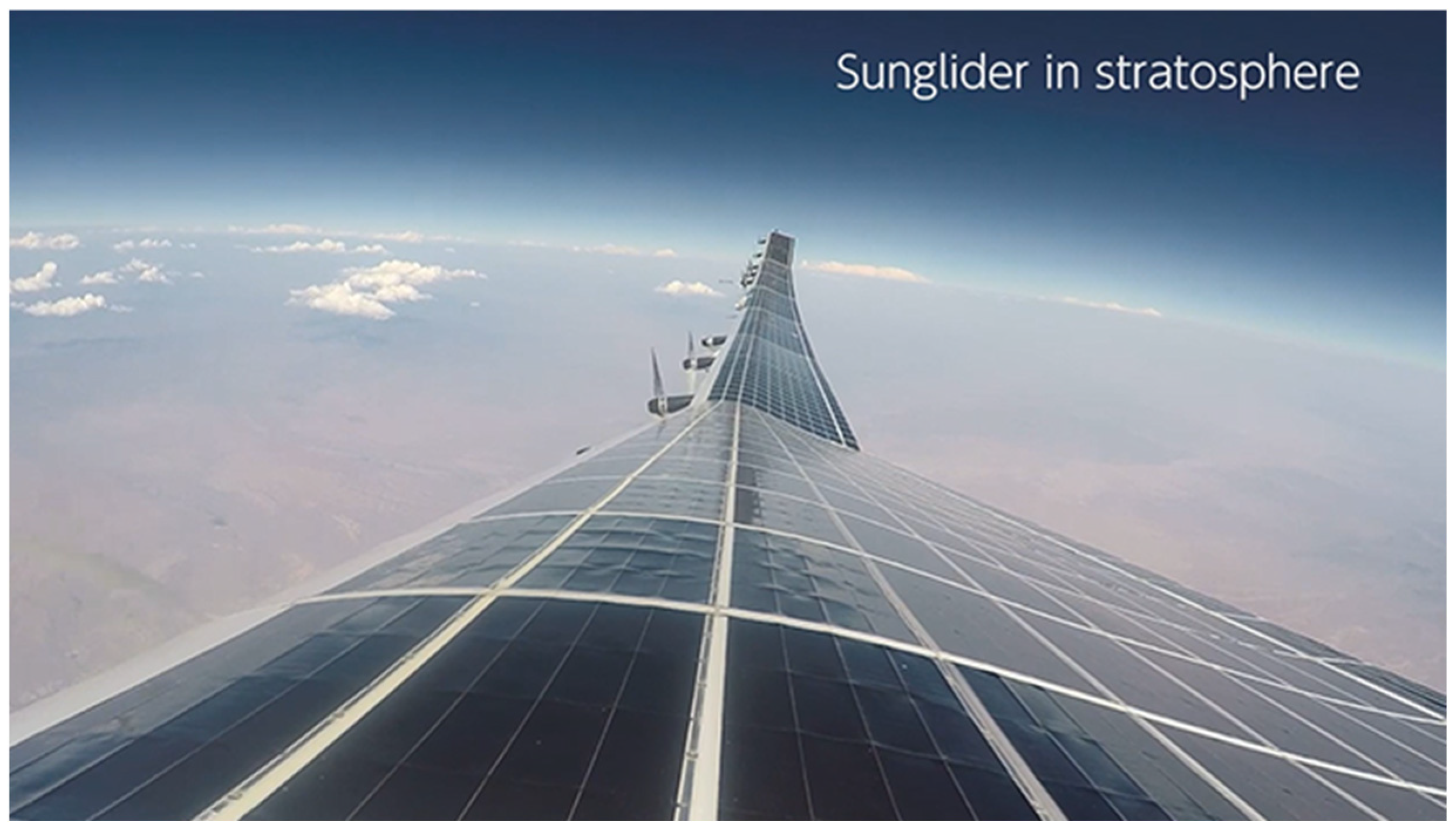
The photovoltaic modules mounted on the upper surface of the HAPS wing are arranged to conform to the curved shape, prioritizing aerodynamic performance (see Figure 1) [33]. Due to this constraint, each solar cell on the module surface has a different normal vector. The cosine loss caused by increased incidence angles and self-shading from the airframe structure varies dynamically with position and time. Consequently, the solar irradiance on the array surface is highly non-uniform [26]. This results in a significant discrepancy between the global horizontal irradiance incident on the aircraft’s projected area and the effective irradiance actually received by the PV system [34].

Especially in stratospheric operations, aircraft altitude, solar position vector, and three-axis flight attitude (roll, pitch, and yaw) interact. Calculations that account for self-shading by airframe components such as main wings, tail wings, and fuselage are therefore required. In this study, we use a curved-surface representation based on differential geometry, as established in our previous report [22]. The core description of this method is as follows.

Generally, studies on vehicle-integrated PVs report that non-uniform radiation intensity on curved PV modules causes current mismatch between cells, known as mismatch loss [35]. Unlike terrestrial environments, where diffuse light predominates, the stratosphere receives direct solar radiation and has a high albedo. In this setting, the contrast from self-shading on curved surfaces is exceptionally high, and the impact of mismatch becomes more severe and complex. This mismatch loss is a critical factor in the energy balance of HAPS operating with a limited light-receiving area.

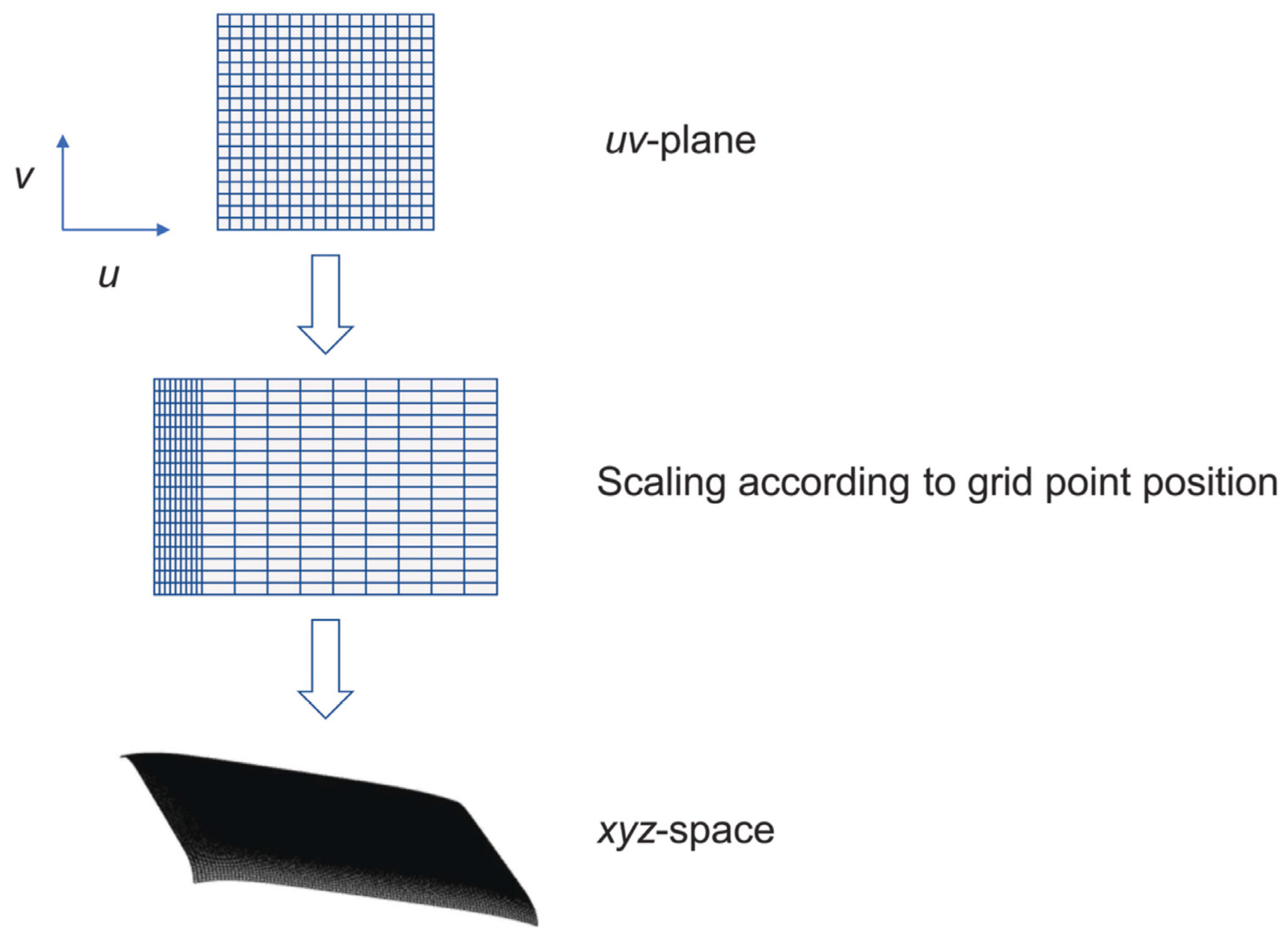
The mathematical expression for the curved surface is defined by a nested matrix, where each element is a vector of position in Cartesian coordinates. To numerically analyze complex light-receiving behavior, this study defines the airframe surface as a mapping from parameter space (uv-plane) to real space (X, Y, Z). The equation serves as a mathematical model that converts grid point information on the u v-plane, held as a two-dimensional array, into a three-dimensional airframe shape. A schematic expression is illustrated in Figure 2. The address of each element is shown in the uv-plane. To obtain optical properties, such as cosine loss and self-shading loss, we compute the first derivative in each direction as a function of (u, v), corresponding to the position of the element. The map file, which allocates the positions of the solar cells on the wings, and differentiates the surface element if it is a simple self-shading surface or not, maintains the same address in the uv-plane [36].

Analyzing this requires surface elements, normal vectors, and first derivatives with respect to each parameter on each curved surface. To describe the complex wing geometry in three-dimensional space, the parametric form representation shown in the following equation is suitable [22].

$$S\left(u,v\right)=\left[\begin{array}{c}x\left(u,v\right)\\ y\left(u,v\right)\\ z\left(u,v\right)\end{array}\right]$$

(19)

In regions such as the leading edge and wingtips of HAPS, the curvature becomes locally steep. As a result, there is a possibility that the change in normal vectors cannot be sufficiently captured with an equally spaced grid. Therefore, this model uses a variable-mesh structure. It arranges grid points non-uniformly on the uv-plane based on the physical curvature distribution.

Geometric physical quantities, such as normal vectors and area elements, are calculated at each grid point. These calculations use the central difference method with adjacent points on the parameter space [22].

$$S_{u,i,j}=\left[\begin{array}{c}{S}_{0,i,j}-S_{0,i+2,j}\\ S_{1,i,j}-S_{1,i+2,j}\\ S_{2,i,j}-S_{2,i+2,j}\end{array}\right]$$

(20)

$$S_{v,i,j}=\left[\begin{array}{c}{S}_{0,i,j}-S_{0,i,j+2}\\ S_{1,i,j}-S_{1,i,j+2}\\ S_{2,i,j}-S_{2,i,j+2}\end{array}\right]$$

(21)

Here, the obtained $S_{u,i,j}$ and $S_{v,i,j}$j are $3\times 1$ column vectors, stored as elements in a matrix having rows and columns corresponding to the total number of grid points. These represent the partial derivative vectors in the $u$ direction and $v$ direction in the parameter space ($u$v-plane). Also, $S$ indicates the specific coordinate values of the airframe surface in $XYZ$ space. That is, for the indices (row number $j$, column number $i$) corresponding to each grid point on the $uv$-plane, the coordinate values of $x,y,z$ are held as matrix elements. The first, second, and third elements of each column vector correspond to the $x,y,z$ coordinates, respectively.

To evaluate the total power generation efficiency of HAPSs, it is necessary to accurately determine the effective surface area of the PV modules deployed on the airframe. This is obtained by integrating minute planar elements (surface elements) over the entire curved surface. The area of the surface element $s_{i,j}$ and the local normal vector $n_{i,j}$ at that point are calculated using the following Equations (22) and (23) [22].

$$s_{i,j}=\left|S_{u,i,j}\times S_{v,i,j}\right|$$

(22)

$$n_{i,j}={\displaystyle \frac{S_{u,i,j}\times S_{v,i,j}}{s_{i,j}}}$$

(23)

Here, $s$ and $s$ denote matrices whose entries are the area and normal vector at each point on the entire airframe surface. Since $S_u$ and $S_v$ are vector quantities, the operator × means the cross product (vector product). Here, $S_u$ and $S_v$ are nested matrices whose elements are vectors calculated using the central difference method for the sides of the pixels in the $u$ direction and $u$ direction based on the 3D mesh of the airframe. The vector obtained by the cross product of these is perpendicular to the tangent plane formed by the original two vectors, and this defines the normal vector of the surface element. Finally, the orientation at each point on the curved surface is defined by normalizing the normal vector n to unit length.

In the calculation of cosine loss, the inner product of the normal vector of each surface element and the incident ray vector is integrated using Equations (22) and (23). For general aircraft shapes with no extreme concavities (i.e., complex multiple-surface regions with multiple peaks), such as HAPS wing surfaces and fuselages, it is possible to determine geometric self-shading from the sign of the normal vector and its inner product with the ray vector. Surface elements where the result of the inner product becomes zero or less are considered such that the component itself becomes a shadow, and the ray does not reach it. Specifically, these geometric relationships are defined as logical values by the following equations.

After the airframe shape and the normal vector of each surface element are defined, it is necessary to compute the ray vector of each component and evaluate the incidence-angle characteristics. In this model, many ray vectors in three-dimensional space are generated based on the spherical coordinate system. These are converted into the x, y, and z components of the orthogonal coordinate system for efficient vector operations, and then processed according to Equation (24) [22].

$$n{n}_k=\left[\begin{array}{c}sin\alpha \cdot sin\zeta \\ cos\alpha \cdot sin\zeta \\ cos\zeta \end{array}\right]$$

(24)

$$S{C}_{i,j}^k=n_{i,j}\cdot n{n}_k$$

(25)

$$S{S}_{i,j}^k=\left(n_{i,j}\cdot n{n}_k>0\right)$$

(26)

Here, $n{n}_k$ is a $3\times 1$ vector indicating the direction of the incident ray to the PV module, having a zenith angle $\zeta$ and an azimuth angle $\alpha$ Based on the Monte Carlo ray-tracing method, $\zeta$ is generated as a random number uniformly distributed in the range of $0°~90°$, and $\alpha$ in the range of $0°~360°$ The index $k$ identifies the random number set generated in the simulation, and $k=\mathrm{1,000,000}$ rays are used to ensure sufficient statistical convergence and reproducibility.

$SC$ and $SS$ are matrices storing the local cosine value and the logical value indicating the presence of self-shading, respectively. A value of 1 (TRUE) is stored for points without self-shading (lit points), and 0 (FALSE) for points in shadow.

2.4. 4-Tensor

The attitude of the HAPS is described by three Euler angles: roll ($\varphi$), pitch ($\theta$), and yaw ($\psi$). To transform the solar vector $S\_global$, defined in the ground coordinate system (Global Frame), into the vector $S\_local$ in the airframe fixed coordinate system (Body Frame), a coordinate transformation matrix $R$ is used. In this study, we adopted the standard $ZYX$ rotation order (Yaw to Pitch to Roll) used in aerodynamics. The coordinate transformation matrix $R$ is defined using the rotation matrices $R_z$, $R_y$, $R_x$ around each axis as follows [31]:

$$R\left(\varphi ,\theta ,\psi \right)={\left(R_z\left(\psi \right)R_y\left(\theta \right)R_x\left(\varphi \right)\right)}^T=R_x{\left(\varphi \right)}^T{R}_y{\left(\theta \right)}^T{R}_z{\left(\psi \right)}^T$$

(27)

$$\begin{gathered} R_x\left(\varphi \right)=\left[\begin{array}{ccc}1& 0& 0\\ 0& cos\varphi & sin\varphi \\ 0& -sin\varphi & cos\varphi \end{array}\right], R_y\left(\theta \right)=\left[\begin{array}{ccc}cos\theta & 0& -sin\theta \\ 0& 1& 0\\ sin\theta & 0& cos\theta \end{array}\right], \\ {R}_z\left(\psi \right)=\left[\begin{array}{ccc}cos\psi & sin\psi & 0\\ -sin\psi & cos\psi & 0\\ 0& 0& 1\end{array}\right] \end{gathered}$$

(28)

Using this rotation matrix, the solar vector $S\_local\left(t\right)$ in the airframe coordinate system at an arbitrary time $t$ is calculated by the following equation [31]:

$$S\_local\left(t\right) = R\left(\varphi \left(t\right),\theta \left(t\right),\psi \left(t\right)\right)·S\_global\left(t\right)$$

(29)

By calculating the dot product of this $S\_local$ and the normal vector $n_{i,j}$ of each mesh on the airframe surface, the incidence angle and the reference index for the 4-tensor are determined. This vector-operation-based approach allows for robust simulation of 360-degree attitude changes while avoiding gimbal lock.

Furthermore, to account for the aeroelastic deformation of high-aspect-ratio wings, this model defines the local deformation angle (deflection) at a position $u,v$ on the airframe as $\varphi \left(u,v,t\right)$. This is derived via spline interpolation of measurements from roll sensors distributed along the wing span. The local solar vector $S_{elastic}$ considering this deformation, is calculated by dynamically adding the deformation angle $\delta \varphi$ to the attitude angle $\varphi \left(t\right)$ of the entire airframe as follows:

$$S_{elastic}\left(u,v,t\right)=R\left(\varphi \left(t\right)+\delta \varphi \left(u,v,t\right),\theta \left(t\right),\psi \left(t\right)\right)\cdot S_{g}lobal\left(t\right)$$

(30)

When the main wing of a HAPS has a saddle-shaped curved surface or complex multiple curvatures, the “Hidden Surface” problem arises in geometric calculations: the solar vector “penetrates” the airframe structure and a hit is detected on the back surface, which should be physically in shadow. To resolve this, we implemented the following Interior Point Detection algorithm for each surface element (quadrilateral mesh). Let the vertex position vectors of the surface element be $P_1,P_2,P_3,P_4$ (counter-clockwise), and let $q$ be the point on the ray vector or its extension to be tested. Also, let $r$ be the unit normal vector of the surface element whether point $q$ lies inside the surface element is determined by computing the cross product of each edge vector with the vector from the vertex to point q, and checking whether the result has the same direction (positive correlation) as the normal vector. That is, if all four conditional expressions below are satisfied, the point is determined to be an Interior Point [36]:

$$\left[\left(p_{i+1}- p_i\right)\times \left(q - p_i\right)\right]\cdot r > 0$$

(31)

Note that $P_5=P_1$. This geometric determination enables the accurate identification of the boundaries of dynamic shadows in complex airframe shapes. Also, note that Equation (31) should be applied to every combination of the index i and the indices of a pair of surface elements. For example, if the surface of HAPS or HAPS wings is covered by 1000 × 1000 elements, the total number of trials for Equation (31) will be 4 × (1000 × 1000)² = 4 × 10¹², including the calculation of the inner product of three-dimensional vectors and the cross product of vectors. At the same time, these vector operations on a large matrix require significant computational time to search for elements within the matrix. Also, these calculations should, in principle, be performed for each ray and each surface element, so the total computation time will be huge. This study extends the concept of the 4-tensor proposed in previous research [17] to accommodate dynamic three-axis attitude changes and HAPS-specific flexible wing deformation. It implements it within a high-speed computational framework. This is to process a structure with four degrees of freedom, obtained by combining two degrees of freedom for angular change with two for positional change, without increasing computational load during execution.

The light-receiving characteristics on a curved wing correspond to two indices (extent of parameter space) describing the surface. They are formulated as a 4-tensor $MM$ having a nested structure as shown in Equations (32) and (33) [22,36,37]. Since a 4-tensor is a four-dimensional structure, and it is not suitable for graphical explanation in principle, we believe the best explanation is made by the form of the nested matrix described in Equation (32). Each element of each nested matrix in the 4-tensor described in Equation (33) is a dimensionless real number with the range of 0 ≤ x ≤ 1, namely [0,1]. It is not a simple cosine loss ratio; it also accounts for the hidden-surface loss ratio [37,38].

$$MM=\left[\begin{array}{ccccc}{M}_{\mathrm{0,0}}& \dots & M_{0,l}& \dots & M_{0,N-1}\\ ⋮& \ddots & ⋮& \ddots & ⋮\\ M_{k,0}& \dots & M_{k,l}& \dots & M_{k,N-1}\\ ⋮& \ddots & ⋮& \ddots & ⋮\\ M_{N-\mathrm{1,0}}& \dots & M_{N-1,l}& \dots & M_{N-1,N-1}\end{array}\right]$$

(32)

$$M_{k,l}=\left[\begin{array}{ccccc}{m}_{\mathrm{0,0}}& \dots & m_{0,j}& \dots & m_{0,N-1}\\ ⋮& \ddots & ⋮& \ddots & ⋮\\ m_{i,0}& \dots & m_{i,j}& \dots & m_{i,N-1}\\ ⋮& \ddots & ⋮& \ddots & ⋮\\ m_{N-\mathrm{1,0}}& \dots & m_{N-1,j}& \dots & m_{N-1,N-1}\end{array}\right]$$

(33)

Here, $M_{k,l}$ is a matrix storing the two-dimensional angular response of the surface element at position $(k,l)$, and $m_{i,j}$ is its scalar element. Generally, the number of elements in a 4-dimensional tensor becomes enormous (e.g., if each matrix is $100\times 100$, the total number of elements is ${10}^8$). Therefore, it is highly inefficient to recalculate whenever the solar position or airframe attitude changes. Thus, in this study, we adopted an algorithm that pre-calculates (catalogs) a reference tensor. During simulation execution, the performance of each surface element is computed using a tensor reference, applying 3D rotation matrices for pitch, roll, and yaw, and then integrated at the module level. Although the ray distribution matrix for each surface element varies in a complex manner with position on the curved surface, this cataloging method minimizes computational cost. For the actual angular deviation, an immediate calculation method using two-dimensional spline interpolation, such as Bicubic Interpolation, was adopted. The motion of the airframe and the sun can be regarded as a rotational transformation of this 4-tensor, thereby achieving both physical rigor and substantial computational speedup in dynamic power-generation simulations in the stratosphere.

Using 4-tensors rather than repeating vector calculations each time appears to reduce total computation time. Although the HAPS flight attitude is dynamic, it affects the ray distributions on the aircraft body’s surface elements. This effect on the 4-tensor can be easily reproduced by rotational coordinate conversion using Equations (28) and (29), without repeating the time-consuming calculation or the accompanying search for matrix elements.

2.5. Power Generation Calculation

By integrating the 4-tensor derived in the previous sections with stratospheric meteorological parameters, the total power generated by the HAPS is calculated. In this study, a high-precision energy balance evaluation accounting for partial shading and temperature non-uniformity is achieved by integrating solar irradiance calculations for each mesh and detailed power-generation characteristics for each solar cell. The power generation $PfP\left(k,t\right)$ at an arbitrary time step $t$ and surface element $k$ (mesh address $jpv$) is calculated according to the following process.

First, the incident irradiance intensity $I\left(k,t\right)$ at the panel element is calculated by the geometric calculation using the 4-tensor. The base power generation $P_{base}$ corresponding to the incident irradiance intensity is expressed by the following equation:

$$P_{base}\left(k,t\right)= I\left(k,t\right)\cdot {\displaystyle \frac{P_{src}}{I_{AM}}}·N_{size}(k)$$

(34)

Here, $P_{src}$ represents the rated output of a standard single cell in the AM0 environment, $I_{AM}$ represents the extra-terrestrial solar irradiance intensity (solar constant), and $N_{size}\left(k\right)$ represents the total series-parallel number of cells included in the array.

Next, to correct for the fluctuation in conversion efficiency associated with the extremely low-temperature environment of the stratosphere and pressure changes, a temperature correction factor $F_{temp}$ and a voltage correction factor $F_{volt}$ are introduced.

Temperature correction factor $F_{temp}$:

$$F_{temp}(k,t)= 1 - \alpha \cdot \left(T_{amb}(t)- T_{ref} + k_{therm} \cdot {\displaystyle \frac{I\left(k,t\right)}{I_0}}\right)$$

(35)

Here, $\alpha$ is the temperature coefficient, $T_{amb}$ is the ambient temperature, $T_{ref}$ is the reference temperature, $I_0$ is the standard solar irradiance (non-zero positive value), and $k_{therm}$ is the thermal coefficient indicating the cell temperature rise according to the irradiance intensity. These parameters were set based on the thermal characteristics of lightweight photovoltaic modules suitable for stratospheric platforms.

Voltage correction factor $F_{volt}$:

$$F_{volt}(k,t)={\displaystyle \frac{V_{ref} + V_{th} \cdot ln\left(\frac{I\left(k,t\right)}{I_0}\right)}{V_{ref}}}$$

(36)

This equation simulates the logarithmic decrease in the open-circuit voltage ($V_{oc}$) under low illumination, based on a physical model (the one-diode model).

Here, $V_{ref}$ is the open-circuit voltage at reference irradiance, and $V_{th}$ is a physical constant corresponding to the thermal voltage. This accurately reproduces the drop in efficiency in low-light environments, where only stratospheric albedo is available.

Finally, the power generation $PfP$ at surface element $k$ is obtained by the following equation:

$$PfP\left(k,t\right)=\left\{\begin{array}{cc}\hfill P_{base}\left(k,t\right)·F_{temp}(k,t)·F_{volt}(k,t), & \left(I\right(k,t)>0\hfill \\ \hfill 0, & \left(I\right(k,t)\le 0\hfill \end{array}\right.$$

(37)

The total generated power $P_{total}\left(t\right)$ of the entire airframe is obtained by summing this over all panels $N_{mesh}$ pieces) [19,32].

$$P_{total}(t)=\sum _{k=1}^{N_{mesh}}PfP\left(k,t\right)$$

(38)

This formulation enables extremely high-precision power generation prediction that reflects the low-temperature, low-pressure environment characteristic of the stratosphere and the dynamic solar-irradiance distribution associated with changes in airframe attitude.

3. Results

In this section, we evaluate the performance of the high-speed computational framework based on the 4-tensor method developed in Section 2 and demonstrate its effectiveness. First, we demonstrate the method’s suitability for long-term simulations by comparing its computational speed with that of conventional methods. Next, we verify the model’s physical validity and accuracy by comparing it with measurement data obtained during stratospheric flight. Finally, using the established model, we analyze energy behavior across a wide range of roll attitudes, from level flight to maximum bank. This reveals the overestimation of energy inherent in conventional planar approximation models and discusses potential energy risks overlooked in operational planning.

3.1. Computational Speed

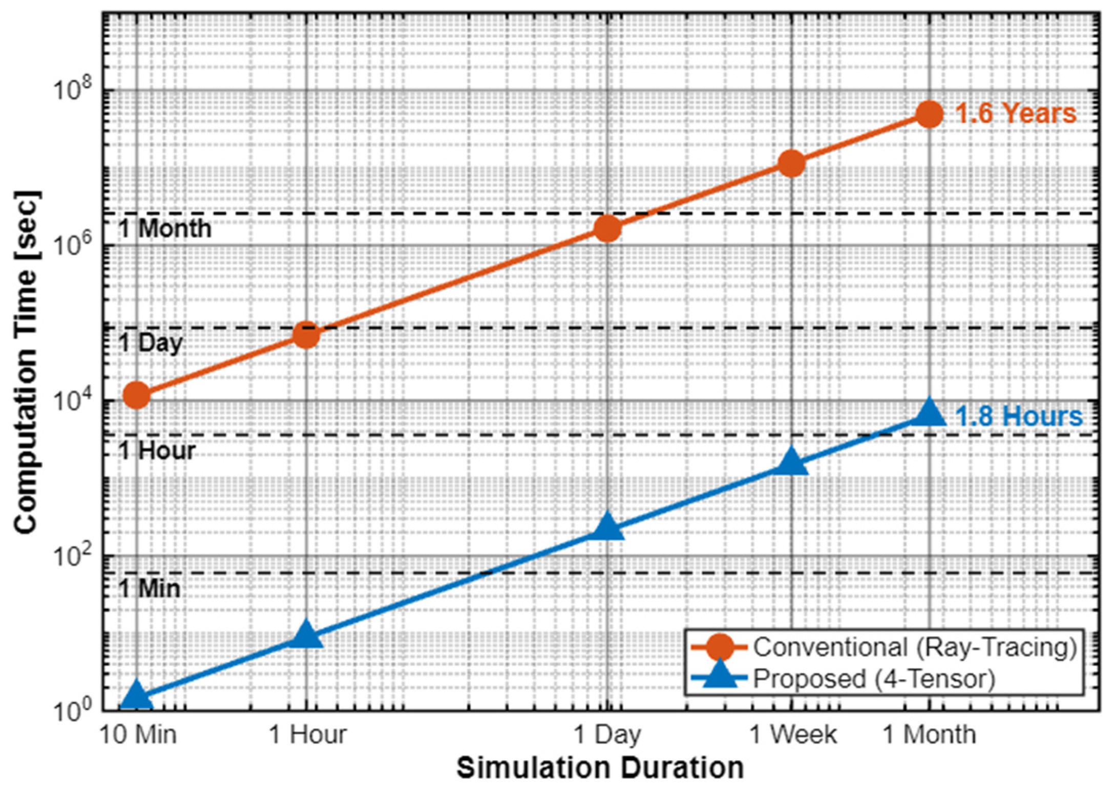
In HAPS energy management, power generation prediction simulations have been a bottleneck for formulating operational plans and optimizing airframe design. Figure 3 compares the computational cost of the 4-tensor method proposed in this study with conventional Monte Carlo ray tracing. The comparison was performed under the same computer environment. It assumes a one-month continuous HAPS flight and plots the transition in computation time relative to the simulation duration on a logarithmic scale.

Looking at the results of the conventional method (red line), computation time increases linearly with the simulation duration. However, the slope is extremely steep. In this traditional approach, whenever the solar position or airframe attitude changes, millions of ray tracing calculations on the airframe surface must be performed. Shadow intersections are determined each time. As a result, approximately 19.2 days (about 460 h) of computation time are required to simulate just one day of flight. This means the real-time simulation is about 20 times longer. Such costs make feedback for daily operational planning virtually impossible. They also hinder conducting numerous case studies, like Monte Carlo simulations under varying weather conditions and flight routes.

In contrast, the 4-tensor method introduced in this study (blue line) demonstrates a substantial performance improvement. In this method, complex geometric calculations that depend on the airframe shape (e.g., self-shading and incidence-angle characteristics) are cataloged in advance as a “4-tensor”. During simulation execution, calculations are reduced to simple matrix operations that reference values for airframe attitude and solar position from this catalog and perform necessary interpolation. As a result, a one-day calculation takes about 3.5 min, and even a one-month analysis can be completed in about 1.8 h. This is a speedup of thousands of times compared with the conventional method, indicating that annual energy balance prediction throughout the HAPS operation cycle and battery capacity optimization studies are now feasible within a practical timeframe.

3.2. Validation Using Flight Data

In this section, we first simulate the stratospheric solar radiation environment at a specific location (Miyazaki) to confirm its basic characteristics. Subsequently, we verify the model’s validity by comparing it with actual flight test data.

3.2.1. Solar Irradiance Simulation in a Stratospheric Environment

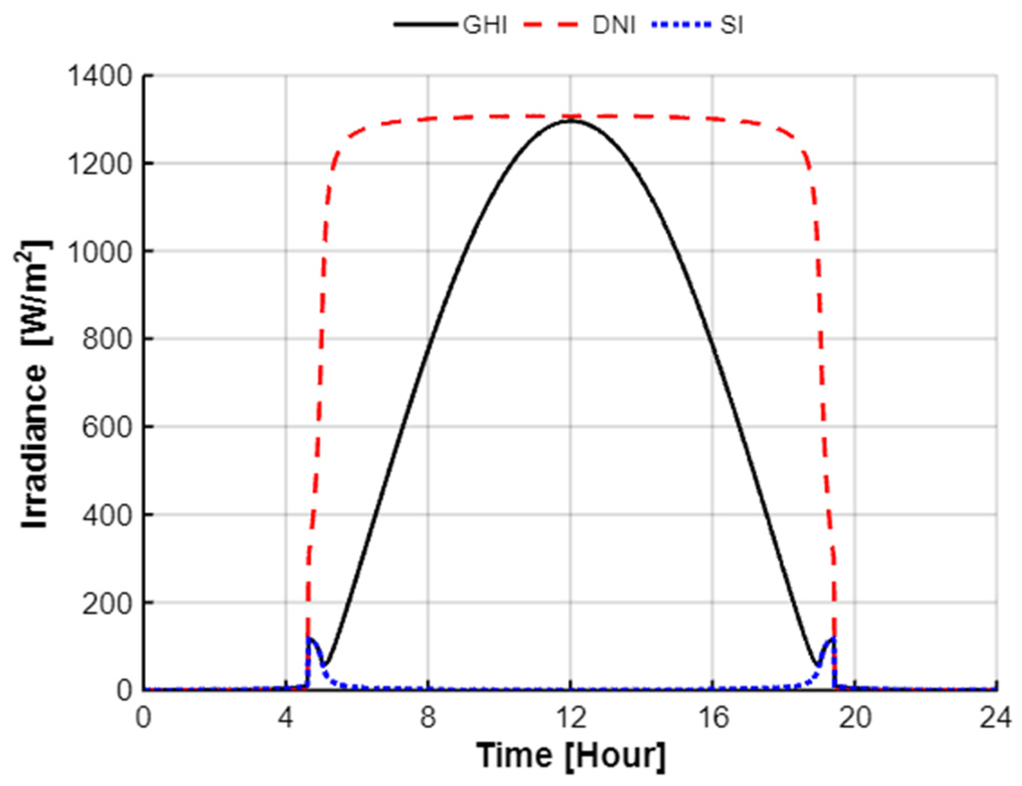
First, as a baseline for the operational environment assumed in this study, a solar irradiance simulation was conducted for the summer solstice (June 21) over Miyazaki Prefecture, Japan. Figure 4 shows the diurnal variation of the solar irradiance components calculated. The solid line (black) in the graph represents Global Horizontal Irradiance (GHI). The dashed line (red) represents Direct Normal Irradiance (DNI). The dotted line (blue) represents Scattered Irradiance (SI).

A notable result is the behavior of DNI. In the terrestrial environment, solar intensity decreases significantly in the morning and evening due to changes in air mass. However, at stratospheric altitudes, where air density is only a few percent of that at ground level, the attenuation effect is extremely limited. As a result, DNI maintains a high value of approximately 1360 W/m² consistently from immediately after sunrise to just before sunset, exhibiting a “rectangular wave-like” profile.

On the other hand, SI, the scattered component, remains at an extremely low value throughout the entire period. This confirms that the influence of scattering by atmospheric molecules and aerosols is limited. This simulation result quantitatively demonstrates that the stratosphere is a “direct-light dominant” environment. It implies that, although the benefits of diffuse ground-level light are not expected, a highly intense energy source (DNI) is available even at low solar altitudes in the morning and evening. Therefore, to effectively utilize this unique “rectangular wave-like” energy, a geometric approach that accounts for three-dimensional attitude control and airframe shape is indispensable. This is rather than the conventional mindset premised on horizontal installation.

3.2.2. Model Validation Using Actual Flight Data

We verified the physical validity and accuracy of the proposed model by comparing it with actual flight test data obtained in stratospheric airspace. For the simulation, time-series data on time, latitude, longitude, altitude, and the airframe’s three-axis attitude (roll, pitch, yaw) from the actual flight recorder were used as inputs.

In this verification, we focused on the output of a specific solar panel. We compared the measured and calculated values against the actual flight data. The target airframe in this study uses flexible photovoltaic modules that conform to the wing’s curved shape.

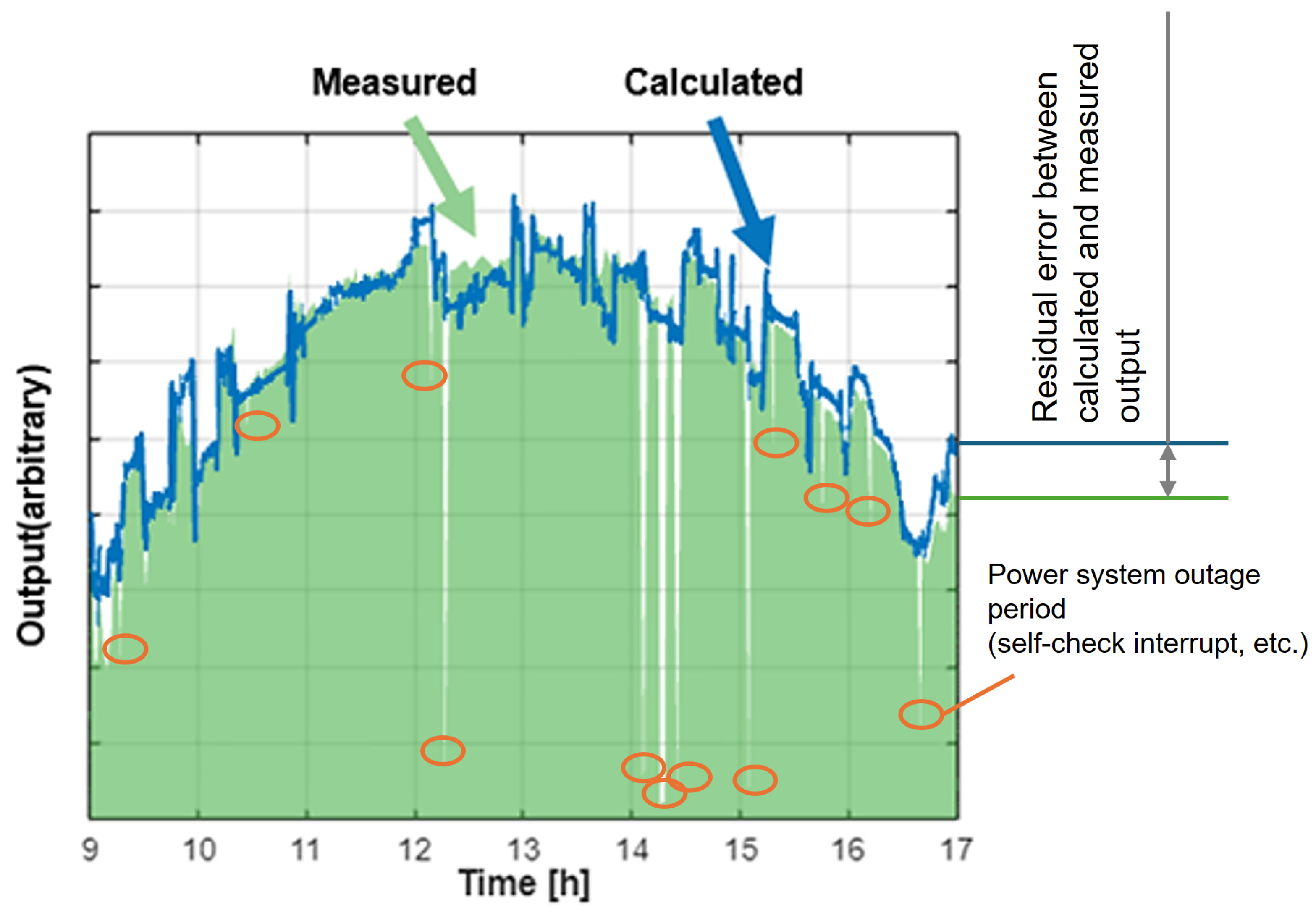
As shown in Figure 5, the proposed model’s results (blue line) consistently reproduce the minute fluctuations observed in the measured values (green area) with high precision. The characteristic output behavior observed in this graph can be explained by the complex interaction between stratospheric-specific environmental conditions and airframe dynamics, as reported in the previous study [18].

The stratospheric environment has extremely few clouds and aerosols, making it “direct-light dominant.” The mitigation effect of diffuse light observed on the ground does not apply here. Therefore, photovoltaic modules mounted on a curved surface exhibit a highly sensitive response to changes in airframe attitude. Particularly at low altitudes immediately after sunrise or sunset, even a slight change in roll angle causes a nonlinear change in the light distribution (shadow area) on the curved surface. This results in large output fluctuations.

In addition to these geometric fluctuations, aerodynamic damping decreases at an altitude of 20 km, where the atmosphere is thin. The airframe flies while experiencing minute attitude fluctuations of about 1° to 2°. The high-frequency spike-like fluctuations seen in the measured values are not sensor noise. Instead, they are the physical result of mechanical micro-vibrations being amplified under a sensitive light-receiving environment. The fact that this model captures even these minute behaviors indicates that the proposed method has high temporal resolution and physical fidelity.

3.3. Analysis of “Structural Overestimation” Due to Roll Attitude Variation

When HAPS performs station-keeping in the stratosphere, the airframe inevitably adopts a roll angle (bank angle) to counteract wind direction or to carry out loiter maneuvers. During this turning operation, the solar panels on the main wing may turn away from the sun or cast shadows due to their shape. This makes this phase critical for predicting the energy balance.

In this section, a simulation was performed for the winter solstice (22 December) as a representative winter scenario with low solar altitude. Specifically, a geometric arrangement was assumed in which sunlight is incident from directly to the side of the airframe, with a relative azimuth difference of 90 degrees. This condition was chosen because the difference between the planar and curved models is most pronounced under these circumstances.

The geometric models used in this verification are defined below. The conventional planar approximation model (Flat Model), used for comparison, is shown in Figure 6. The curved-surface model (Curved Model) of the proposed method is illustrated in Figure 7. The curved model in this study is constructed from airframe data for a practical HAPS assumed to operate in the stratosphere [33]. We performed calculations using the same tensor and matrix sizes and the same number of index-searching cycles, even for large matrices. As discussed in Section 2.4, we believe the computation time is mainly due to the large number of vector–product operations and the element searching algorithm in large matrices. Keeping the matrices geometrically simple and of the same size allows us to clearly compare and demonstrate the advantages of our developed computation framework.

By considering the large deflection caused by the flexible structure of the airframe, as well as the camber inherent to the airfoil, the “saddle-shaped geometry”—defined in the previous report—was faithfully reproduced as a parametric curved surface. This approach allows for an accurate capture of the effects of “self-shading” and local incidence angles. These effects vary intricately with surface position, whereas conventional planar approximations ignore them.

Reference [23] reported that in a direct-light-dominant stratospheric environment, the contrast between light and dark at the shadow boundary becomes pronounced. Power output fluctuates sharply with minor changes in the airframe’s attitude. Conventional flat-plate models and static analyses with coarse time resolution often average out and overlook these subtle behaviors. However, the strong agreement between this calculation result and observed physical phenomena confirms that the proposed method is highly accurate. It can immediately reflect minute changes in the energy balance. In the analysis, the roll angle was continuously varied from 0 degrees (level) to 90 degrees (vertical). The power generation characteristics during this process were verified.

In our research, we did not compare or compete in accuracy with other published research algorithms, including a ray tracing simulation. We believe that comparing several algorithms without sufficient validation with actual flight data are essential. In this regard, we do not believe we need to perform additional calculations beyond those used by existing algorithms that have also been examined in the history of VIPV research.

Absolute dimensional information for the aircraft body, solar cell sizes, and wing shape may be of interest to some readers. However, this information also constitutes non-public data pertaining to the design and manufacturing of the HAPS aircraft and cannot be disclosed. However, the calculations presented in this paper are performed using geometric data converted from the XYZ coordinate system to the uv (parametric) space. Additionally, solar radiation intensity and power generation are processed by area, establishing a proportional relationship that eliminates the need for absolute dimensions for model verification. Furthermore, the three-dimensional figures depicted are rendered without distorting the relative positional relationships, thereby preserving geometric similarity.

3.4. Energy Overestimation by Planar Approximation

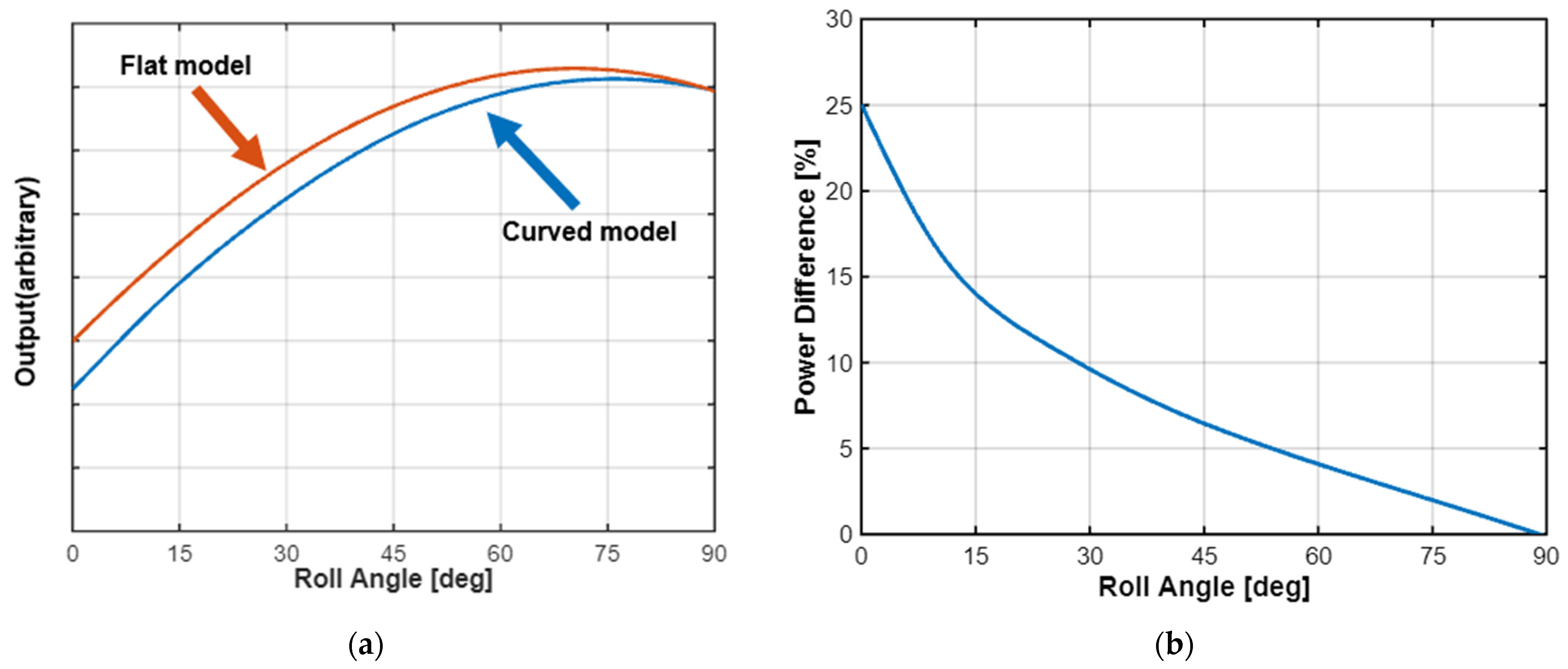
The graph in Figure 8 shows the transition in power generation efficiency as a function of roll angle under the above conditions. The red line represents the flat model, and the blue line represents the curved model. Overall, power generation increases with roll angle in both models. Specifically, the flat model shows a peak at approximately 70°, whereas the curved model shows a peak at approximately 75°. This difference in peak position of about 5° is attributed not only to the simple module installation angle but also to the continuous change in normal vectors along the curved surface. While the flat model has a uniform light-receiving surface along the chord line, the curved model has a curved surface. Therefore, even at an angle (75°) past the peak of the flat model, the curved model maintains a situation where a part of the curved surface directly faces the sun (peak). In other words, this result suggests that the curved model accurately captured the “local optimal light-receiving angle” which is averaged and overlooked by planar approximation, and as a result, the peak position shifted to the higher angle side.

A quantitative comparison of the two models’ predicted values showed that the curved model (blue line) consistently lies below the flat model (red line) across the entire region, and the degree of overestimation varies significantly with the operating mode. The largest difference was observed during level flight (roll angle 0°), e normal cruising state.

Under this condition, although the incidence angle is shallow, the flat model calculates that “the entire area of the wing receives light without being in shadow.” In contrast, in the curved model, due to the wing’s camber (curvature) and the deflection of the saddle shape, the opposite side of the sun is self-shaded over a wide area, creating a region where power generation is physically impossible.

The analysis revealed a discrepancy between the “calculated light-receiving area” and the “effective light-receiving area,” indicating that the flat model overestimates power generation by approximately 25% relative to the actual state (curved model) during level flight. Furthermore, this overestimation persists even when the bank angle is increased. According to the analysis, within the normal range up to a roll angle of 20°, which is frequently used for 20° normal turning and course correction, an estimation error of more than 12% still persists. This means that, in daily operations, the flat model continues to account for more than 10% of “non-existent energy,” a fatal error in the long term.

Additionally, even at a roll angle of 70°, where the bank angle is deepened toward the sun and power generation is maximized, this overestimation is not fully resolved. Even in this region where the incidence angle is optimized, an output decrease of about 3% still remains due to the influence of “self-shading,” where the bulge of the wing itself shields the rear cells and the incidence angle loss at the wing tips. At first glance, the difference appears slight, but in the winter solstice operation in the stratosphere, where the energy balance is close to the limit, a loss of a few percent can be decisive for nighttime survivability.

This study revealed that this “large discrepancy in level/normal range (10–25%)” and “hidden loss at optimal attitude (3%)” by the flat model lead to fatal Energy Overestimation in the operational planning of HAPSs. If an operational plan was based on a conventional flat model, a double calculation error would occur: the accumulated value of base power during the day would be largely insufficient, and, furthermore, the expected value would not be reached even during the evening sun-chasing, the final spurt. This lack of predictive accuracy directly leads to the failure to achieve a full battery charge for night flight and to the loss of the airframe (Loss of Control) due to power depletion before dawn. Therefore, it is concluded that the introduction of this method, which accurately estimates losses arising from wing thickness and curvature, is indispensable for ensuring a reliable operational plan with a safety margin.

4. Discussion

In this section, based on the numerical simulations and comparison results with actual flight data presented in Section 3, we discuss the validity of the proposed method. We also examine the power generation characteristics in the stratospheric environment and explore the engineering implications for practical operation.

4.1. Effectiveness of Introducing Curved Model in the Stratospheric Environment

In the analysis in Section 3.3, it became clear that the degree of overestimation by the planar approximation model varies dynamically with the airframe’s roll angle, which is the incidence angle with respect to the sun. The discrepancy is most pronounced during normal-level flight, with roll angles between 0° and 30°. During this state, the solar altitude is low, and the incidence angle to the wing becomes extremely shallow. Although the planar model calculates that the entire wing receives light even in this state, the actual curved wing behaves differently. Light at a shallow angle is blocked by the bulge on the near side, causing severe self-shading across a wide area. Furthermore, most of the curved surface does not face the sunlight directly, and the effective light-receiving area decreases significantly. This combination of increased self-shading and decreased light-receiving efficiency results in a substantial prediction error of up to 25% compared to the planar model. In contrast, when the airframe tilts significantly toward the sun to achieve the optimal attitude —where power generation is maximized—at a roll angle of approximately 75°, this error decreases dramatically to approximately 3%. In this specific angle, the majority of the curved wing (the peak part) faces the sun directly, in the normal direction. Unlike in level flight, even a curved surface can receive direct solar radiation when in this attitude. This minimizes the area that becomes self-shaded. As a result, the deviation in predictions appears to have converged as the system approaches the state of full surface light reception assumed by the planar model. The physical characteristic that “the shallower the incidence angle, the larger the error” indicates a risk influenced not only by airframe attitude but also by the time of day. During periods around sunrise and sunset, when solar altitude is extremely low, self-shading effects are maximized, as they are during level flight. This makes the overestimation by the planar model significant. In the daily energy balance, the evening—when energy output is at its last spurt, and the morning when charging begins—are critical phases. Accounting for “energy that does not actually exist” in these time zones risks misleading decisions about transitioning to night flight. From these observations, it is clear that the planar model fails to capture losses specific to curved surfaces at shallow incidence angles during level or low-bank attitudes, and at low altitudes during morning and evening. These conditions account for most operational time. The concentration of prediction errors within these normal and important ranges poses a serious risk for battery capacity planning. Therefore, correction using accurate curved-surface calculations is indispensable.

4.2. Contribution to Computational Efficiency and Operation Optimization

One of the major contributions of this study is that, by implementing the 4-tensor method, power generation calculations that strictly account for curved shapes were dramatically accelerated without compromising physical fidelity. Pilots and operators who remotely control from the ground must predict the airframe’s energy balance in real time. This prediction is necessary in response to rapidly changing weather conditions and sudden mission changes. With conventional methods, calculations could not keep up. As a result, they relied on rules of thumb or simple estimations. However, using this method, it is possible to simulate tens of thousands of flight patterns in real time on a high-performance ground-based computer. This allows immediate derivation of the optimal attitude and route to avoid self-shading. In other words, this study provides a powerful tool to evolve HAPS operations. It shifts from static, prior-planning-based approaches to dynamic energy management that can respond immediately to changing conditions.

4.3. Platform-Independent Versatility and Extension to LTA

The essential value of the 4-tensor method proposed in this study lies in its purely geometric nature. It is independent of specific airframe shapes or flight dynamics models. Many conventional simplified models are premised on the wing planform of fixed-wing aircraft. This makes it difficult to adapt them to other HAPS platforms with significantly different shapes [7,8,10]. However, because this method uses only the 3D mesh information of the airframe surface and its normal vector distribution as input variables, power generation can be calculated using the same algorithm regardless of the target. The target could be a fixed-wing aircraft (Heavier-Than-Air: HTA), or an airship or balloon (Lighter-Than-Air: LTA).

In other words, this method is not limited to a single airframe analysis tool. It can serve as a standard framework for energy evaluation across the entire next-generation Non-Terrestrial Network (NTN). In this network, a wide variety of forms—from HTA to LTA—coexist. Although a demonstration targeting the HTA type was conducted this time, this mathematical framework is applicable to the design optimization of all stratospheric platforms.

4.4. Computational Scaling and Surface Modeling Considerations

Since the majority of computation time is allocated to large-scale matrix search operations, it is reasonable to establish that the relationship between computational speed and problem size follows a proportional law. In other words, the calculation time increases linearly with the size of the matrix or tensor, while the trade-off between accuracy and computational effort remains consistent with the mesh dimensions.

This algorithm uses a four-dimensional tensor to account for hidden-surface considerations, addressing several prior limitations. Unlike earlier methods that relied solely on the inner product between normal vectors and light-ray vectors—such as those used to model convex surfaces—it can be applied to other exotic curved surfaces, such as saddle-shaped wings, without neglecting the shadow effects of stabilizer wings and propellers. This approach provides a more comprehensive solution.

The algorithm presumes that curved surfaces can be effectively represented through surface models. While it is true that converting triangular mesh data obtained from handheld 3D scanners into such models may introduce geometric inaccuracies, this issue is part of the broader scope of 3D geometric modeling. Nonetheless, it is crucial to acknowledge this potential source of error when applying the method.

4.5. Environmental Variability and Its Impact on Tensor-Driven Power Output Calculations

The 4-tensor itself is a geometric quantity uniquely determined by the surface’s geometric conditions, so it is not affected by albedo or atmospheric conditions. Therefore, it is not necessary to recalculate when the Albedo or atmospheric conditions change. In the actual calculation of solar radiation distribution, each element of the 4-tensor is multiplied by the intensity of the rays, so the resulting intensity is strongly influenced by albedo and atmospheric conditions.

For the 4-tensor, the effects of wing flapping under high-altitude conditions and strong stratospheric winds must be carefully considered. However, it is difficult and unrealistic to accurately predict the coordinates of the wing surfaces associated with these deformations. In fact, the effect is small compared to changes in the aircraft’s pitch, roll, and yaw angles. In this calculation, local fluctuations in pitch, roll, and yaw angles were corrected using a Bicubic Interpolation function for the measured flapping amount, so that these variations could be captured as much as possible. The calculation time associated with this is much shorter than the calculation time for tensor generation, so once cataloging tensors, fully benefit from them.

It is assumed that the dynamic effect on the power generation output of albedo and other plants will be affected by the rise and fall of the troposphere, especially in the troposphere. Since the flight in this study was in sunny weather, the calculated values were in good agreement with the flight data, as shown in Figure 4. However, in cloudy weather, the power output of curved solar cells in HAPSs is strongly affected by cloud reflection and ground surface reflections. Furthermore, in stratospheric flight, the error is thought to increase in regions where the absolute value of the pitch angle is large, as it is affected by reflected light from Earth’s surface (including cloud and sea surfaces). Also, in the HAPS design with solar panels on the wings’ backsides, the total power from the PV will be affected by albedo and other solar conditions.

5. Conclusions

In this study, to achieve persistent flight of HAPSs and avoid the risk of airframe loss from excessive energy estimates using conventional planar approximation models, we developed a high-speed power generation prediction framework. This framework accurately reproduces output spikes associated with airframe attitude variations. The main findings from the verification are described below.

First is the dramatic improvement in computational efficiency. We implemented a method that predefines and represents complex vector operations in curved PV analysis as a 4-tensor. This significantly reduces the computational load compared to conventional methods such as ray tracing. As a result, long-term energy balance analysis, which traditionally requires substantial time, could be conducted within a practical timeframe—approximately 1.8 h for a one-month operation simulation. This enables long-term energy management throughout the operation cycle.

Second is the reproducibility of output fluctuations associated with airframe oscillation. Compared with actual stratospheric flight data, the proposed model accurately captures the steep, spike-like fluctuations in power generation caused by minute changes in airframe attitude. This demonstrates that the model physically and accurately describes the changes in incidence angle received by each cell on the curved surface. This is especially relevant in the stratospheric environment, where direct solar radiation dominates.

Third, the analysis identified a risk of overestimating energy with the planar approximation model. The conventional planar model overestimates power generation by approximately 25% during level flight. This discrepancy persists at about 12% even during routine turns with a roll angle of 20° and is not fully resolved at the optimal angle. Such overestimation is a significant risk factor. It is directly linked to battery-charging failures during night flights and to the potential loss of the airframe—commonly referred to as Loss of Control—due to power depletion before dawn. This model is an essential tool for correcting structural prediction errors and establishing safe operational limits to prevent crashes.

In conclusion, the method developed in this study achieves both accuracy and speed in long-term energy prediction for HAPS operations. It is versatile across diverse stratospheric platforms, including fixed-wing aircraft and airships. This innovation is expected to serve as a core technology for autonomous flight control and predictive maintenance, supporting next-generation communication infrastructure.

References

1. Karapantazis, S.; Pavlidou, F.-N. Broadband communications via high-altitude platforms: A survey. IEEE Commun. Surv. Tutor. 2005, 7, 2–31. [Google Scholar] [CrossRef] [Scilit]
2. Kurt, G.K.; Khoshkholgh, M.G.; Alfattani, S.; Ibrahim, A.; Darwish, T.S.J.; Alam, M.S.; Yanikomeroglu, H.; Yongacoglu, A. A Vision and Framework for the High Altitude Platform Station (HAPS) Networks of the Future. IEEE Commun. Surv. Tutor. 2021, 23, 729–779. [Google Scholar] [CrossRef] [Scilit]
3. D’Oliveira, F.A.; De Melo, F.C.L.; Devezas, T.C. High-altitude platforms-Present situation and technology trends. J. Aerosp. Technol. Manag. 2016, 8, 249–262. [Google Scholar] [CrossRef] [Scilit]
4. Kanchanasut, K.; Tsuchimoto, Y.; Das, D.K.; Tunpan, A.; Wongsaardsakul, T.; Awal, M.A. DUMBONET: A multimedia communication system for collaborative emergency response operations in disaster-affected areas. Int. J. Emerg. Manag. 2007, 4, 670. [Google Scholar] [CrossRef] [Scilit]
5. 3GPP. Study on New Radio (NR) to Support Non-Terrestrial Networks (NTN); Technical Report TR 38.811 V15.4.0; 3rd Generation Partnership Project (3GPP): Sophia Antipolis, France, 2020; Available online: https://portal.3gpp.org/desktopmodules/Specifications/SpecificationDetails.aspx?specificationId=3234 (accessed on 16 February 2026).
6. Aglietti, G.S.; Markvart, T.; Redi, S.; Tatnall, A.R. Harnessing High-Altitude Solar Power. IEEE Trans. Energy Convers. 2009, 24, 442–451. [Google Scholar] [CrossRef] [Scilit]
7. Arum, S.C.; Grace, D.; Mitchell, P.D.; Zakaria, M.D.; Morozs, N. Energy Management of Solar-Powered Aircraft-Based High Altitude Platform for Wireless Communications. Electronics 2020, 9, 179. [Google Scholar] [CrossRef] [Scilit]
8. Gao, X.-Z.; Hou, Z.-X.; Guo, Z.; Liu, J.-X.; Chen, X.-Q. Energy Management Strategy for Solar-powered High-altitude Long-endurance Aircraft. Energy Convers. Manag. 2013, 70, 20–30. [Google Scholar] [CrossRef] [Scilit]
9. Dai, Q.; Xing, D.; Fang, X.; Zhao, Y. Conceptual Design of an Energy System for High Altitude Airships Considering Thermal Effect. Energies 2021, 14, 4204. [Google Scholar] [CrossRef] [Scilit]
10. Noth, A. Design of Solar Powered Airplanes for Continuous Flight. Ph.D. Thesis, ETH Zurich, Zurich, Switzerland, 2008. Available online: https://www.researchgate.net/publication/251502667_Design_of_Solar_Powered_Airplanes_for_Continuous_Flight (accessed on 16 February 2026).
11. Oettershagen, P.; Melzer, A.; Mantel, T.; Rudin, K.; Stastny, T.; Wawrzacz, B.; Hinzmann, T.; Leutenegger, S.; Alexis, K.; Siegwart, R. Design of small hand-launched solar-powered UAVs: From concept study to a multi-day world endurance record flight. J. Field Robot. 2017, 34, 1352–1377. [Google Scholar] [CrossRef] [Scilit]
12. Suh, H.; Lee, S. Energy-Efficient Trajectory Optimization for Solar-Powered UAVs using Gravity Potential Energy. Aerospace 2022, 9, 765. [Google Scholar] [CrossRef] [Scilit]
13. Aragón-Zavala, A.; Delgado-Penín, J.A.; Cuevas-Ruíz, J.L. High-Altitude Platforms for Wireless Communications; Wiley: Hoboken, NJ, USA, 2008. [Google Scholar] [CrossRef] [Scilit]
14. Patil, M.J.; Hodges, D.H.; Cesnik, C.E.S. Nonlinear aeroelastic analysis of high-aspect-ratio wings. J. Aircr. 2001, 38, 88–96. [Google Scholar] [CrossRef] [Scilit]
15. Wang, H.; Song, B.; Zuo, L. Effect of High-Altitude Airship’s Attitude on Performance of its Energy System. J. Aircr. 2007, 44, 2077–2080. [Google Scholar] [CrossRef] [Scilit]
16. Duffie, J.A.; Beckman, W.A. Solar Engineering of Thermal Processes, 4th ed.; Wiley: Hoboken, NJ, USA, 2013. [Google Scholar] [CrossRef] [Scilit]
17. Herrero, R.; Antón, I.; Martín, F.; Askins, S.; Macías, J.; José, L.J.S.; Vallerotto, G.; Núñez, R.; Domínguez, C. Indoor and Outdoor Evaluation of Curved Modules for VIPV. In Proceedings of the 2023 IEEE 50th Photovoltaic Specialists Conference (PVSC), San Juan, PR, USA, 11–16 June 2023; pp. 1–3. [Google Scholar] [CrossRef] [Scilit]
18. Tian, X.; Lu, Y.; Wang, J.; Lu, G.; Jiang, M.; Khan, S.A.; Ji, J.; Luo, C. Modeling and Analysis of Flexible Curved PV Cells under Uneven Irradiation considering Varied Parameters. Energy 2025, 328, 136655. [Google Scholar] [CrossRef] [Scilit]
19. Gloeckner, P.; Rodway, C. The Evolution of Reliability and Efficiency of Aerospace Bearing Systems. Engineering 2017, 9, 962–991. [Google Scholar] [CrossRef]
20. Song, K.; Li, Z.; Zhang, Y.; Wang, X.; Xu, G.; Zhang, X. Power Generation Calculation Model and Validation of Solar Array on Stratospheric Airships. Energies 2023, 16, 7106. [Google Scholar] [CrossRef] [Scilit]
21. Foley, J.D.; van Dam, A.; Feiner, S.K.; Hughes, J.F. Computer Graphics: Principles and Practice, 2nd ed.; Addison-Wesley: Reading, MA, USA, 1995. [Google Scholar]
22. Araki, K.; Ota, Y.; Nishioka, K. Vector-Based Advanced Computation for Photovoltaic Devices and Arrays: Numerical Reproduction of Unusual Behaviors of Curved Photovoltaic Devices. Appl. Sci. 2024, 14, 4855. [Google Scholar] [CrossRef] [Scilit]
23. Mukai, N.; Araki, K.; Nishioka, K.; Okada, K.; Ota, Y. Development of total energy simulator for high altitude platform station operation. Sol. Energy Mater. Sol. Cells 2026, 296, 114054. [Google Scholar] [CrossRef] [Scilit]
24. Hoshino, K.; Ohta, Y.; Sudo, S. A Study on Antenna Beamforming Method Considering Movement of Solar Plane in HAPS System. In Proceedings of the 2019 IEEE 90th Vehicular Technology Conference (VTC2019-Fall), Honolulu, HI, USA, 22–25 September 2019; pp. 1–5. [Google Scholar] [CrossRef] [Scilit]
25. Liu, Y.; Sun, K.; Xu, Z.; Lv, M. Energy efficiency assessment of photovoltaic array on the stratospheric airship under partial shading conditions. Appl. Energy 2022, 325, 119898. [Google Scholar] [CrossRef] [Scilit]
26. Smith, M.J.; Patil, M.J.; Hodges, D.H. CFD-based analysis of nonlinear aeroelastic behavior of high-aspect ratio wings. In Proceedings of the 19th AIAA Applied Aerodynamics Conference, Anaheim, CA, USA, 11–14 June 2001. AIAA 2001-1582. [Google Scholar] [CrossRef] [Scilit]
27. Iqbal, M. An Introduction to Solar Radiation; Academic Press: Toronto, ON, Canada, 1983. [Google Scholar]
28. ICAO. Manual of the ICAO Standard Atmosphere (Extended to 80 Kilometres (262 500 Feet)), 3rd ed.; Doc 7488-CD; International Civil Aviation Organization: Montreal, QC, Canada, 1993. [Google Scholar]
29. National Renewable Energy Laboratory (NREL). Solar Spectral Resource. Available online: https://www2.nrel.gov/grid/solar-resource/spectral (accessed on 15 January 2026).
30. Spencer, J.W. Fourier series representation of the position of the sun. Search 1971, 2, 172. [Google Scholar]
31. Kasten, F.; Young, A.T. Revised optical air mass tables and approximation formula. Appl. Opt. 1989, 28, 4735–4737. [Google Scholar] [CrossRef] [Scilit]
32. Press, W.H.; Teukolsky, S.A.; Vetterling, W.T.; Flannery, B.P. Numerical Recipes: The Art of Scientific Computing, 3rd ed.; Cambridge University Press: Cambridge, UK, 2007. [Google Scholar]
33. SoftBank Corp. Stratospheric Communications Platform HAPS. Available online: https://www.softbank.jp/corp/philosophy/technology/special/ntn-solution/haps/ (accessed on 15 January 2026).
34. Araki, K.; Ota, Y.; Nagaoka, A.; Nishioka, K. 3D Solar Irradiance Model for Non-Uniform Shading Environments Using Shading (Aperture) Matrix Enhanced by Local Coordinate System. Energies 2023, 16, 4414. [Google Scholar] [CrossRef] [Scilit]
35. Tayagaki, T.; Yoshita, M.; Sasaki, A.; Shimura, H. Comparative Study of Power Generation in Curved Photovoltaic Modules of Series- and Parallel-Connected Solar Cells. IEEE J. Photovolt. 2021, 11, 708–714. [Google Scholar] [CrossRef] [Scilit]
36. Araki, K.; Matsushita, S.; Ota, Y.; Iwasaki, S.; Hosokawa, Y.; Nishioka, K. Rating Vehicle-integrated Photovoltaics: Power and Energy Loss by Curved Surface. Sol. Energy Mater. Sol. Cells 2025, 292, 113814. [Google Scholar] [CrossRef] [Scilit]
37. Matsushita, S.; Araki, K.; Ota, Y.; Nishioka, K. Evaluation of Incident Light Characteristics for Vehicle-Integrated Photovoltaics Installed on Roofs and Hoods Across All Types of Vehicles: A Case Study of Commercial Passenger Vehicles. Appl. Sci. 2025, 15, 8702. [Google Scholar] [CrossRef] [Scilit]
38. SoftBank Corp. High-Precision Power Generation Simulation for Solar-Powered HAPS. Available online: https://www.softbank.jp/corp/technology/research/topics/089/ (accessed on 15 January 2026).
Figure 1. Wing of a HAPS shape [33].
Applsci 16 02183 g001
Figure 2. Parametric representation of the curved surface [36].
Applsci 16 02183 g002
Figure 3. Comparison of computation time between the conventional method (ray tracing) and the proposed method (4-tensor).
Applsci 16 02183 g003
Figure 4. Simulation results of solar irradiance components during the summer solstice in the stratosphere.
Applsci 16 02183 g004
Figure 5. Validation of the proposed model using actual flight data. The blue solid line represents the calculated power–output trend. The green painted region represents the measured power output. Details of the flight history (Date, Place, PV configuration, etc.) are protected by the HAPS manufacturer and flight operators.
Applsci 16 02183 g005
Figure 6. Conventional flat plate approximation model used as a comparison baseline.
Applsci 16 02183 g006
Figure 7. Parametric curved surface model of the proposed method based on actual HAPS geometry [38].
Applsci 16 02183 g007
Figure 8. (a) Comparison of power generation characteristics against roll attitude variation; (b) Quantitative analysis of Energy Overestimation by the planar approximation model.
Applsci 16 02183 g008
Disclaimer/Publisher’s Note: The statements, opinions and data contained in all publications are solely those of the individual author(s) and contributor(s) and not of MDPI and/or the editor(s). MDPI and/or the editor(s) disclaim responsibility for any injury to people or property resulting from any ideas, methods, instructions or products referred to in the content.