Boundary-Focused Large Language Model Adaptation for Style Change Detection in Multi-Authored Text

Abstract

The style change detection (SCD) task involves identifying the locations of writing style changes in multi-authored documents. This task can be applied to plagiarism detection, security, and commerce applications. Introducing decoder-based Large Language Models (LLMs) marks a pivotal shift in applications. The segment boundaries for SCD models can be represented by concatenating two consecutive segments as pairs. However, LLMs usually restrict their input lengths, where the long-length inputs may exceed the restricted length. This paper seeks to bridge this gap and exploit the power of LLMs by introducing boundary-focused LLM Adaptation for SCD (BF-LLMA-SCD). The proposed solution adapts decoder-based LLMs for SCD using QLoRA. BF-LLMA-SCD truncates long-length input by preserving texts near an examined boundary while removing those at the other sides. BF-LLMA-SCD was trained on three PAN datasets. Comparison results with the top-performing SOTA solutions show that BF-LLMA-SCD achieved the best performance results in terms of F₁ on PAN 2021 and PAN 2022/D1, while obtaining competitive results on PAN 2022/D3. BF-LLMA-SCD was also trained on an Arabic SCD dataset comprising three difficulty levels. It achieved an F₁ score above 0.99 on easy instances.

1. Introduction

Natural languages serve as the fundamental medium for human communication that enables the transmission of knowledge and the expression of human ideas. The writing language varies from person to person. Thus, each author has linguistic characteristics reflected in their writing, which is referred to as their unique writing style. With the increasing availability of textual data, there has been a growing demand to differentiate between the styles of authors who collaborate on a document. Analyzing linguistic characteristics helps differentiate author styles for addressing tasks related to computational linguistics and security applications to detect suspicious documents. The demand for forensic linguistic and law enforcement applications also motivates work on this task [1,2]. By identifying changes in writing style, the solutions contribute to suggesting potential cases of plagiarism, such as literary plagiarism in historical documents [3]. Another motivation is to evaluate the consistency of writing assistance tools [2]. By detecting style changes, the solutions can assess the coherence of suggested edits made by proofreaders. They can also help institutions adhere to a specific style in their documents. Also, commercial products for writing assistance can involve such solutions to enhance their quality.

A Large Language Model (LLM) is a model built on deep neural networks (DNNs). It is trained using enormous amounts of text data without tuning on specific task data. LLMs have demonstrated significant promise in tackling a range of Natural Language Processing (NLP) tasks, including text classification and natural language understanding [4]. LLMs are characterized by their huge number of learnable parameters, which enables them to learn complex linguistic patterns and semantic relationships. These models can adapt their parameters to better suit a particular task by retraining some or all of them without substantial architectural changes. LLMs are also considered pretrained models, where the initial training is performed on massive and diverse text data. This training helps acquire vast amounts of knowledge. Their capacity can then be generalized to address downstream tasks with less task-specific data than would be required for training from scratch. LLMs usually restrict their input lengths and truncate long inputs that exceed those lengths.

In this paper, we introduce Boundary-Focused LLM Adaptation for SCD (BF-LLMA-SCD) to detect changes in writing styles. To the best of our knowledge, it is the first solution that adapts LLMs with a focus on boundaries for truncating. BF-LLMA-SCD fine-tunes decoder-based LLMs based on Quantization Labeled optimizer Rate Adaptation (QLoRA) [5], which helps reduce resource and time consumption during LLM fine-tuning. Truncating long-length input sequences focuses on text located near boundaries, while removing texts at the other sides. This truncation strategy enables BF-LLMA-SCD to handle more relevant contexts for detecting style changes.

The remainder of this paper is organized as follows: the SCD task is reviewed in Section 2. A detailed overview of the SOTA solutions is presented in Section 3. The proposed solution is described in Section 4. Experimental evaluation and results are presented in Section 5. The findings and suggestions for further directions are summarized in Section 6 to conclude the study.

2. Background

Natural language is composed of words to coin meaningful sentences. It is spoken or written by humans, whereas textual data represents written language. The writing language varies from person to person, depending on the differences in how a language is used in writing. Each author has a unique writing style that is characterized by their language preferences and reflected in their writing. Researchers attempt to identify linguistic features that can be used to measure styles quantitatively to distinguish authors’ writing styles. Several factors can affect writing style. Stylistic features can be directly related to written texts, including lexical, syntactic, and application-specific features. Additionally, the nuances of style may vary according to physiological or psychological states, such as the author’s mood and environmental factors [6]. The writing style of the same author can also evolve over time [7,8]. This section presents the definition of the SCD task and briefly reviews the main characteristics of Arabic texts for this task.

2.1. Task Definition

The SCD task focuses on analyzing a multi-authored document that merges distinctive and inconsistent writing styles in a single document. The SCD task aims to find the locations of authors’ writing style changes in a multi-authored text. It decomposes a multi-authored document into its authorial components by identifying the positions of style changes [9]. The authorial component comprises one or more textual segments, such as a single paragraph or a series of consecutive paragraphs, written by the same author. Thus, in any multi-author document, the position of a change in the writing styles is determined between every authorial component. The distinction between author styles is made without requiring a comparison of previous documents. The SCD task then focuses on identifying style changes within a single document, regardless of whether the text is duplicated in other documents.

The SCD task is associated with a specific language. The PAN Evaluation Laboratory organizes scientific competitions to promote research on stylometry and digital text forensics (https://pan.webis.de, accessed on 14 February 2026). The annual organization of PAN competitions has become an essential event for providing SCD benchmark datasets and developing State-Of-The-Art (SOTA) solutions on English datasets.

Table 1. Example of the SCD task.

	Document 1	Document 2
Author 1	This paragraph was written by the first author.	This paragraph was written by the first author.	Author 1
	This paragraph has two sentences. They were written by the first author.	Two sentences are in this paragraph. The second author wrote both sentences.	Author 2
	This paragraph as well was written by the first author.	The second author wrote this paragraph too.
	This paragraph was also written by the first author.	This paragraph also was written by the first author.	Author 1
Para. level	[0, 0, 0]	[1, 0, 1]
Sent. level	[0, 0, 0, 0]	[1, 0, 0, 1]

shows examples of writing style changes and provides the expected output for the SCD task. Document 1 is a single-authored document, while Document 2 is a multi-authored document written by two authors, with two style changes appearing as lines. SCD’s outcome is a set of binary values related to boundary positions at a specific level. The outcomes in the table are located at the paragraph and sentence levels. A boundary with a value of 1 signifies a change between the segments around it in that they are written by different authors. A boundary with a value of 0 indicates that the same author wrote the segments and they share the same style. As a result, the length of the result is equal to the number of textual components minus 1. As can be seen in Table 1, a unique author wrote document 1, and no style changes were made within its boundaries. The output then is a list of zeros. Document 2 shows that Authors 1 and 2 switch after the first and third paragraphs. Thus, the output after examining Document 2 is a list of two ones that appear at the first and the third indexes, indicating that the changes occur at the first and the third boundaries. At the sentence level, four boundaries exist, and Authors 1 and 2 switch at the first and the fourth sentences. Therefore, the output at the sentence level is a list of two ones appearing at the first and the fourth indexes.

2.2. Arabic Language

Arabic is a Semitic language [10]. It differs from Indo-European languages in terms of alphabet, morphology, and syntax. From an alphabetical perspective, there are twenty-eight Arabic letters. They have contextual variants that can be presented in different shapes depending on their position in words. For example, the letter “ ع ” can be represented as “ عـ ” if the letter appears at the beginning of a word like “ علم ” ([Elm]: know), “ ـعـ ” if it appears in the middle like “ العلم ” ([AlElm]: the knowledge), “ ـع ” if it is at the end like “ قطع ” ([qTE]: cut), or “ ع ” if it appears independent of other letters like “ باع ” ([bAE]: sold). (In this paper, an Arabic word is represented with some or all three components according to context: “Arabic word” ([Buckwalter Arabic transliteration [11]]: English translation).) Moreover, Arabic does not support capitalization, which increases the difficulty of some information extraction and understanding tasks, including SCD.

From a morphology perspective, the Arabic templatic morphology interweaves patterns and affixes to roots [12]. For instance, the word “ الطلاب ” ([AlTlAb]: the students) was coined starting with the root “ طلب ” ([Tlb]: request). Then the pattern “ فعال ” ([fEAl]) is applied to produce “ طلاب ” ([TlAb]: students). Finally, the prefix “ ال ” ([Al]: the) precedes the pattern to get the final word “ الطلاب.” This structure differs from concatenative languages; for example, the English word “the students” is constructed by concatenating “the” and “s” with the word “student”. In some cases, a single Arabic word can represent an entire English sentence. For example, the Arabic word “ فأسقيناكموه ” ([f>sqynAkmwh]: then we give it to you to drink) can be translated into English using eight words.

From a syntactic perspective, several Arabic grammatical rules differ from those of English. Arabic is a relatively free word-order language [10]. The order of sentences can be verb–subject–object, subject–verb–object, or object–verb–subject. Unlike English, Arabic sentences consider syntactic constituency. A noun and its modifiers must correspond in gender, number, and definiteness. In the case of singular or dual, the quantifier and the noun must agree in gender. For example, “ طالبتان اثنتان ” ([TAlbtAn AvntAn]: two female students) is grammatically correct because the word “ اثنتان ” ([AvntAn]: two female) and the word “ طالبتان ” ([AvntAn]: two female students) are feminine. In the case of the plurative, the quantifier and the noun must not agree in gender. For example, the word “ ثلاث ” ([vlAv]: three) and the word “ طالبات ” ([TAlbAt]: female students) in the phrase “ ثلاث طالبات ” ([vlAv TAlbAt]: three female students) disagree in gender. It can also be noted that dual forms are supported in Arabic by concatenating dual pronouns, “ طالبتان ”, which are not present in English, where dual pronouns are typically separate words, “two students”. Moreover, Arabic sentences can be presented without explicitly using a verb as an equivalent to the English verb “to be”. Thus, the Arabic sentence “ أنا الطالب ” ([>nA AlTAlb]: I am a student) and “ أنا هو الطالب ” ([>nA hw AlTAlb]: I am a student) are equivalent and grammatically correct in Arabic.

These Arabic characteristics influence the way authors write their thoughts within linguistic structures. Arabic poetry, for instance, has a unique tradition with distinct meters that differ from those of English poetry. Arabic poetry is more symbolic, incorporates more complex metaphors, and follows more intricate rhyme patterns than English poetry [13].

Table 2. Arabic example of the SCD task.

	Document 1	Document 2
	.هذه الفقرة كتبت من المؤلف الأول	.هذه الفقرة كتبت من المؤلف الأول	Author 1
Author 1	هذه الفقرة تتكون من جملتين. وكتبت كلاهما . من المؤلف الأول	يمكن صياغة الفقرة الثانية من خلال جملتين .منفصلتين حيث قام المؤلف الثاني بكتابتهما	Author 2
	.هذه الفقرة كتبها المؤلف الأول	.هذه الفقرة كتبها المؤلف الأول	Author 1
Para. level	[0, 0]	[1, 1]
Sent. level	[0, 0, 0]	[1, 0, 1]

presents the Arabic example for the SCD task. The presented texts are shown in cursive script from right to left. Two authors wrote the sentences differently in terms of length and structure. The example exhibits style changes similar to those in the English example in Table 1.

3. Related Works

This section provides an overview of the methods incorporated in previous SCD works. According to the conducted review, three methods were adopted: statistical methods, classical machine learning methods, and deep neural network methods [14].

In statistical methods, models were developed by selecting stylistic features, followed by applying statistical estimations without training models [15,16,17]. Khan [15], Khan [16] defined a measure for each type of handcrafted feature, assuming the style has changed if the score is less than a threshold. Karas et al. [17] adopted a distribution test called the Wilcoxon Signed Rank Test [18] to predict style changes.

In classical machine learning (ML) methods, models are obtained based on either supervised or unsupervised learning. Most supervised-based solutions relied on the logistic regression and the random forest algorithms [19,20,21], whereas Support Vector Machine outperformed them in other proposed works, e.g., MAWSA 2018 [22]. Unsupervised learning-based solutions mostly utilized clustering documents based on the similarity of their writing styles using the K-means clustering algorithm [3,20,23,24,25] and the cosine similarity function that outperformed Jaccard and Dice functions [23].

Pretrained-based models are contextualized-based models, including BERT [26], RoBERTa [27], ALBERT [28], ELECTRA [29], DeBERTa [30], mT0-xl [31], ERNIE [32], STAR [33] and sentence-transformer models [34]. BERT-based models were common representation models from 2020 to 2022 [35,36,37,38,39,40,41]. In 2022, Jiang et al. [42] investigated ELECTRA as a type of generative adversarial network architecture to address the absence of the Masked Language Modeling (MLM) task during BERT fine-tuning. In 2023, each solution of DeBERTa-based [43,44,45], RoBERTa-based [46], and mT0-xl-based studies [47] was compared with another solution, which had a similar architecture but was based on BERT, in ablation experiments. The results of these experiments showed that BERT-based models underperformed the other solutions [44,45,46,47]. In 2024, most SCD solutions adopted RoBERTa alone or along with other pretrained models [48,49,50,51,52,53,54,55]. At the same time, STAR [33] and DeBERTa [56,57] were also adopted. For the first time, LLMs were studied for the SCD task in 2024. Lv et al. [58] have explored fine-tuning LLaMA [59] by adapting layers related to the self-attention mechanism. Liang et al. [60] developed a solution based on a teacher–student architecture. They utilized GPT-3 [61] as the teacher model and T5 [62] as the student model. Although transformer models can handle lengths longer than GloVe, they suffer from inconsistency between the training and fine-tuning phases.

In DNN methods, features represent whole documents instead of specific features. Documents were fed into a CNN model [63], a Siamese neural network of one or two BiLSTM layers [22,64]. Other works used pretrained models, such as ELECTRA [42] and BERT with a CNN layer [35,37], an MLM head [36], or feedforward neural networks [38,39]. ECNN-S-SCD [65] is our previous SCD solution, which introduces an Edge Convolutional Neural Network for the Arabic SCD task. It represents boundaries as standalone learnable parameters across layers based on graph neural networks.

4. Proposed Solution: BF-LLMA-SCD

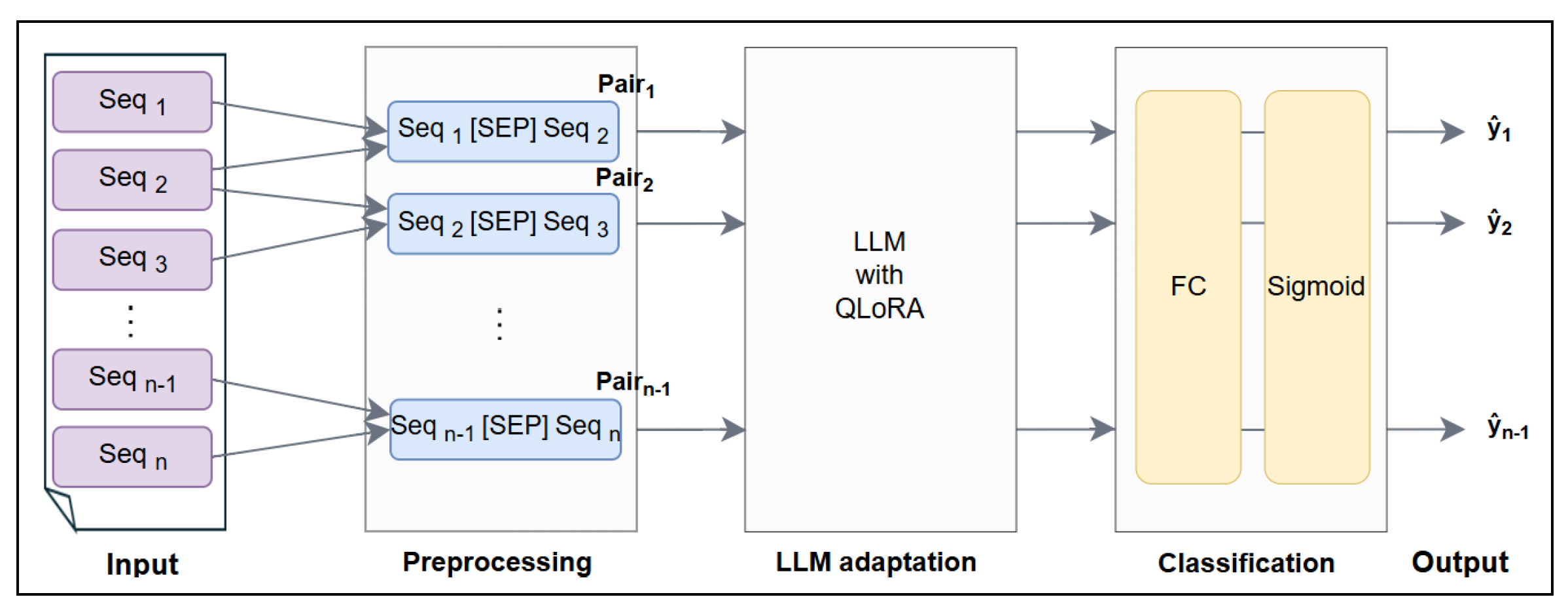
This section describes the development of BF-LLMA-SCD, comprising three main stages: preprocessing, LLM adaptation, and classification. As illustrated in Figure 1, BF-LLMA-SCD receives a document containing a set of input sequences, denoted by $Se{q}_1$ to $Se{q}_n$. These sequences are then passed to the preprocessing stage. Every two consecutive sequences form a pair, generating $n-1$ pairs. These pairs serve as the refined input to the next stage. The LLM Adaptation component is powered by fine-tuning decoder-based LLMs for SCD. This stage generates contextualized representations, which are passed to the classification stage. This stage consists of one Fully Connected (FC) layer followed by the Sigmoid activation function to produce the final predictions ${\widehat{y}}_1$ to ${\widehat{y}}_{n-1}$, which represent the state of the boundary’s style: changed or not changed. Each of these three stages is described in the following subsections.

Table 3. Symbol definitions.

Symbol	Definition
X	F-dimensional embedding matrix for n instances, $X\in R^{n\times F}$
F	A matrix dimension
$F_{in}$	Dimension of input embedding matrix
$F_{out}$	Dimension of output embedding matrix
$W_0$	Original learnable parameters
$W_{0-ft}$	Original learnable parameters after fine-tuning
A	LoRA adaptor matrix
B	LoRA adaptor matrix
r	Rank of lower-rank matrix
$\mathbb{R}$	The set of all real numbers
$\widehat{Y}$	All predicted labels
$\widehat{y}$	A predicted label, $\widehat{y}\in \widehat{Y}$
$Seq$	An input sequence
⊕	Summation operation

summarizes the key symbols used in this paper.

4.1. Preprocessing

One of the straightforward ways to represent a boundary is by concatenating two sequences as a single input separated by a separator token. The input sequences are converted into tokens before being processed. For BF-LLMA-SCD, the input length is 512 tokens, which represents a concatenation of two sequential sequences. Therefore, any input with a length less than 512 tokens will be padded using a special token. In larger cases, one of the truncation strategies can be applied. The only-first truncation strategy is the default one that truncates a token at a time from the first sequence to reach 256 tokens. However, if the length of the first sequence exceeds 512 tokens, only the first 512 tokens of this sequence will be processed, while the second sequence will be discarded. Thus, applying the only-first truncation strategy may lead to losing the boundary’s features and result in an incorrect representation. Therefore, another truncation strategy was applied for BF-LLMA-SCD, known as the boundary-focused strategy [45]. It focuses on boundaries between sequences to enrich the representation of style changes. In contrast to the only-first truncation, this strategy considers both sequences and balances tokens between them. It preserves tokens located nearest to the boundary in both sequences, while discarding the remaining tokens.

Algorithm 1 explains the application of the boundary-focused strategy. It considers a list of documents $Docs$ and the maximum available length used for an LLM $max$. The sequences are converted into tokens before measuring the lengths to perform an accurate truncation operation. The total length of the actual input sequences includes the special symbol $\left[SEP\right]$ in addition to the length of the two sequences. This separator $\left[SEP\right]$ is usually inserted between two sequences to indicate the boundary between them. For BF-LLMA-SCD, it helps the model to learn the separation between two writing styles. Focusing on boundaries during the truncation process occurs only if the total length of the two sequences is greater than the maximum length $max$. Thus, the length of each sequence will be within the average length or less. A pair then contains the two truncated sequences separated by $\left[SEP\right]$. Algorithm 1 returns a list of all pairs for every document in a dataset.

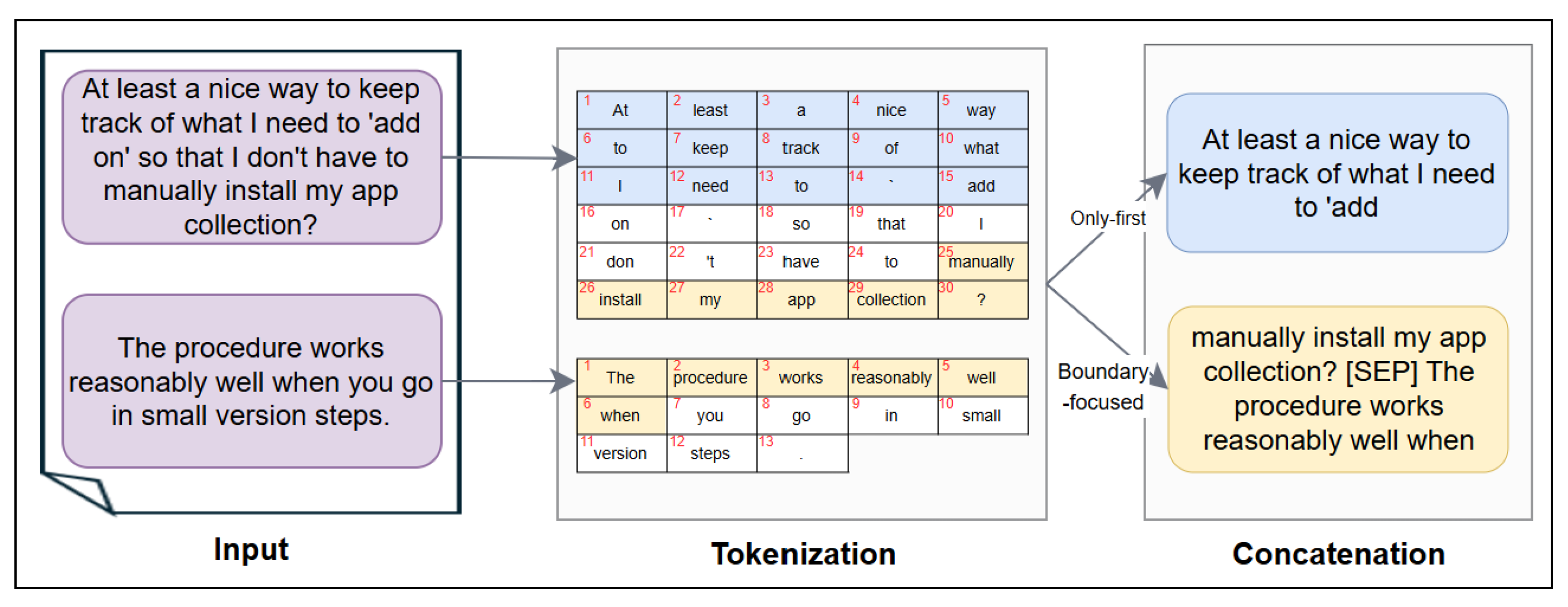
Figure 2 delineates an example of truncating input sequences. For simplification in this example, the maximum length is set to 15. Figure 2 shows two sentences (the sentences were extracted from “PAN 2022/D3 \train \problem-3.txt” [66]) with two truncation strategies: only-first and boundary-focused truncation. The tokenizer used in this example is for LLaMA 3. The only-first truncation results in a pair that contains only the first sequence because the input’s length exceeds 15, potentially overlooking crucial features of the boundary. The blue tokens in Figure 2 represent the tokens selected using the only-first strategy. Conversely, boundary-focused truncation integrates the last six tokens from the first sequence with the first six tokens of the subsequent sequence. This strategy ensures a more consistent representation of the boundary. The yellow tokens in Figure 2 represent the tokens selected by using the boundary-focused strategy.

Algorithm 1 Boundary-focused strategy for BF-LLMA-SCD

Input: $Docs$: A dataset,             $max$: A maximum input length for an LLM, Output: $Pairs$: A list of pairs of sequences for each document in a dataset 1: $Pairs\leftarrow \varnothing$ 2: for all  $doc\in Docs$  do 3:       $Seq\leftarrow$ segmenting_paragraphs ($doc$)                  //Text segmentation 4:       for $i\leftarrow 1$ to |$Seqs$|−1 do 5:            $to{k}_1,to{k}_2\leftarrow$ do_tokenizer($se{q}_i$, $se{q}_{i+1}$) 6:            if (|$to{k}_1$|+|$to{k}_2$| −3 ) > $max$ then 7:                 $avg\leftarrow$${\displaystyle \frac{max-3}{2}}$ 8:                 $to{k}_1\leftarrow to{k}_1[max(1,|to{k}_1|-avg)\dots |to{k}_1\left|\right]$ 9:                 $to{k}_2\leftarrow to{k}_2[1\dots min(|to{k}_2|,avg)]$ 10:                $se{q}_1,se{q}_2\leftarrow$ Undo_tokenizer($to{k}_1$,$to{k}_2$) 11:           end if 12:           $pair\leftarrow$$se{q}_1$+“$\left[SEP\right]$”+$se{q}_2$ 13:           $Pairs$.insert($pair$) 14:      end for 15: end for 16: Return  $Pairs$

4.2. Large Language Model Adaptation

LLaMA [59] was adopted as a pen-source decoder-based LLM. It offers the flexibility of fine-tuning for SCD on all available SCD instances. To mitigate the limitations of requiring intensive resources, the Labeled optimizer Rate Adaptation (LoRA) method is adopted. All original LLM weights $W_0\in$${\mathbb{R}}^{F_{out}\times F_{in}}$ are frozen. Instead, the LoRA adapter is updated, which consists of two weight matrices B and A, where B∈${\mathbb{R}}^{F_{out}\times r}$, A∈${\mathbb{R}}^{r\times F_{in}}$, and the rank r is lower than $F_{out}$ and $F_{in}$, as shown in Equation (1). The initialization values of B are zero, while A uses a random Gaussian initialization.

$$X^{\prime }=W_{0}X+▵WX=W_{0}X+BAX$$

(1)

After training LLMs with LoRA, the resulting A and B matrices are used to get the fine-tuned weight matrices $W_{0-ft}$. The matrix multiplication operation is first performed on A and B matrices for all relevant layers. The resulting matrices are then added to the original weights $W_0$. Thus, the original weight matrices $W_0$ in Equation (1) are replaced by the fine-tuned weight matrices $W_{0-ft}$ in the test phase. Equation (2) shows this final step in the fine-tuning process.

$$X^{\prime }=W_{0-ft}X=(W_0+B\left(AX\right))$$

(2)

To initialize the LoRA adapter, the rank r must be adjusted as a hyperparameter. It represents the number of linearly independent rows (or columns) in a matrix. Linearly independent rows (or columns) occur when they cannot be formed by a combination of other rows (or columns). It is worth noting that the rank is invariant when calculated using either rows or columns [67]. For a lower-rank matrix, the number of linearly independent rows is less than the total number of its rows. This lower-rank matrix is useful for data compression during fine-tuning. To set an optimal r value, Hu et al. [68] have found that small r values led to competitive results, and increasing r values do not obtain significant improvements [68]. Dettmers et al. [5] also showed that the value of r did not affect performance when LoRA was adopted in all LLM layers. Therefore, decreasing r will reduce the number of parameters that must be fine-tuned as well as the memory usage. For BF-LLMA-SCD, the results of preliminary experiments were similar using different r values. Thus, a small r was adopted, which is 8.

Targeted weight matrices in LoRA are hyperparameters. Transformer-based LLMs have four weight matrices in the self-attention module and two in the MLP module. The weight matrices $W_q$, $W_k$, and $W_v$ help transform input data into query, key, and value vectors, respectively, for computing attention scores. The fourth weight matrix $W_o$ plays a role in transforming the output of the attention mechanism into a final output representation. MLP weight matrices apply nonlinear transformations. Although the LoRA adapter can be attached to any weight matrices, the original empirical investigation of Hu et al. [68] for LoRA was conducted to fine-tune the weight matrices of the self-attention module and freeze the MLP modules. Hu et al. [68] found that fine-tuning both $W_q$ and $W_v$ achieved almost similar performance to fine-tuning all four weights. For BF-LLMA-SCD, two weight matrices were adopted: $W_Q$ and $W_V$.

Despite adopting LoRA, BF-LLMA-SCD struggled with training and testing in our computing environment. Thus, Quantization LoRA (QLoRA) was adopted reduce resources and time consumption during LLM fine-tuning. Dettmers et al. [5] introduced different QLoRA approaches, including 4-bit NormalFloat. The NormalFloat is a special data type for compressing a normal distribution of weights from a high-precision format into a smaller one. At the end of this process, the values are restored back to the higher precision. This compression seeks to handle memory efficiently and perform faster computations. Deciding the best value for compression is critical. Dettmers and Zettlemoyer [69] studied quantization for LLMs. They conducted more than 35,000 experiments with 16-bit inputs and different b-bit parameters, including 3, 4, 8, and 16 bits. They showed that adopting 4-bit precision achieved almost optimal accuracy. Therefore, 4-bit precision was adapted for BF-LLMA-SCD.

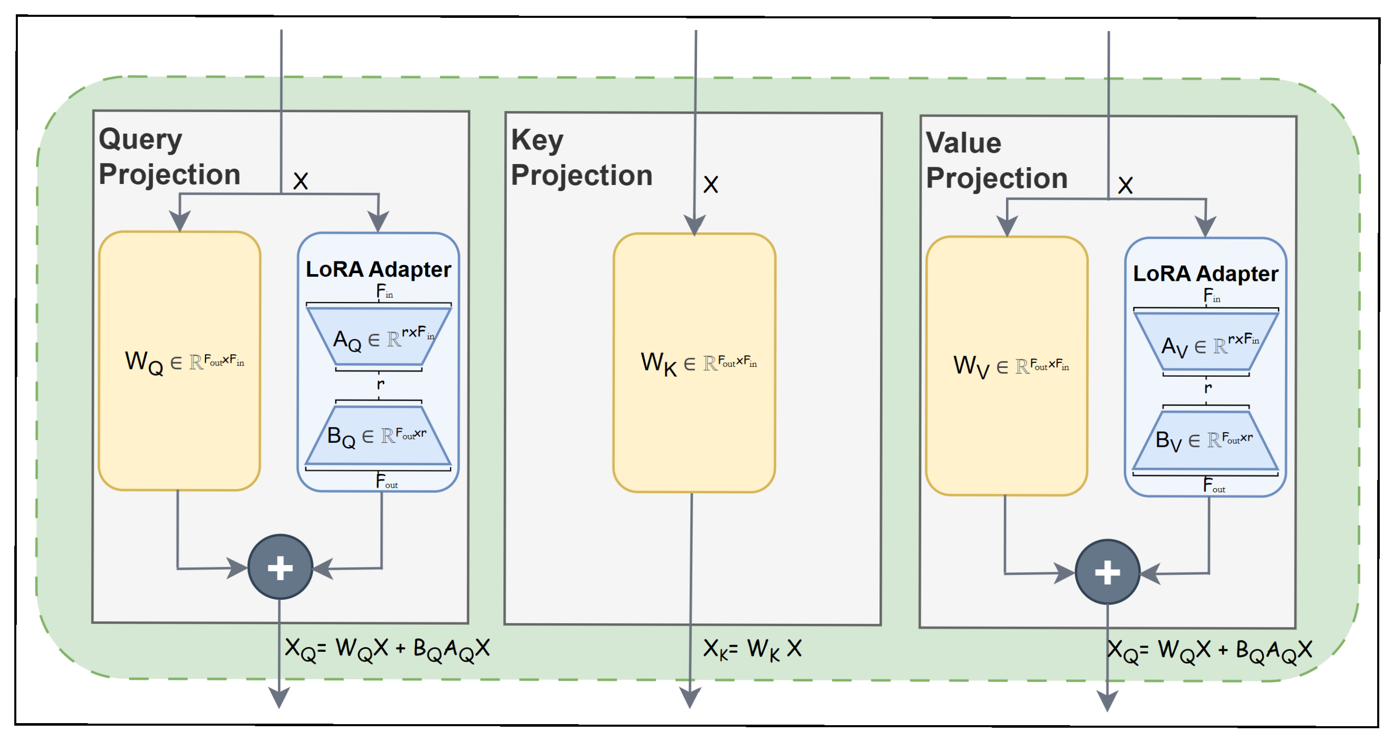
Figure 3 illustrates the self-attention components with LoRA in a single transformer-based LLM layer. It elaborates the architectural flow and focuses on how LoRA was integrated. The process begins with feeding the input embeddings X resulting from the previous layer. This feeding comes in parallel to three distinct linear projection pathways: query, key, and value. The query and value projections demonstrate the application of LoRA. In these two projections, the input embeddings X are passed into two parallel sub-paths. In the first sub-path, the original weights $W_0$∈${\mathbb{R}}^{F_{out}x{F}_{in}}$ are multiplied by X∈${\mathbb{R}}^{F_{in}x1}$, where $W_0$ remains frozen during weight updates. In the second sub-path, the input embeddings X are passed simultaneously through LoRA. It comprises two trainable matrices A and B. A∈${\mathbb{R}}^{r\times F_{in}}$ performs a down-projection, where r $<<$ $F_{in}$. A is represented as an isosceles trapezoid where the shorter parallel side corresponds to the LoRA rank r and the longer parallel side corresponds to the input dimension $F_{in}$. B∈${\mathbb{R}}^{F_{out}\times r}$ performs an up-projection. It is represented as an isosceles trapezoid as well, where the longer parallel side corresponds to the output dimension $F_{out}$. X is first multiplied by A to be in the r dimension, and the result is then multiplied by B to be in the $F_{out}$ dimension. During the forward pass, the output from $W_0$ and the LoRA adapter paths are then element-wise summed via the addition operation represented by ⊕. The resulting matrix is then used for the subsequent attention computation. During the backward pass, gradients are updated only for A and B, where the frozen $W_0$ are not updated.

4.3. Classification

Rich features extracted from a fine-tuned decoder-based LLM are fed into a classification layer. However, such LLMs are primarily designed for text generation, and were trained on the next token prediction task. Hence, such LLMs maintain a contextualized representation for every token, where the last hidden state is represented in a three-dimensional matrix. Therefore, pooling operations can be applied to this matrix to obtain a two-dimensional matrix for SCD.

Although a decoder-based LLM usually does not explicitly contain special tokens to aggregate representations of a sequence, such LLMs can be adopted for SCD by using a last-token method. Example LLMs with left-to-right attention are autoregressive models, which predict the next token in a sequence based on the previous tokens in the same sequence. Hence, the last token’s representations can accumulate the context of the entire sequence. For BF-LLMA-SCD, the last-token method takes the last non-padding token located in the last hidden state.

After that, the pooled representations extracted from the last LLM layers are fed into a classification layer. One FC layer was adopted as it was the most commonly used in SOTA solutions. The Sigmoid activation function was used. It is placed at the final layer before detecting changes using a threshold of 0.5 to round outputs to 0 and 1. It is noteworthy that LLMs provided on the Huggingface (https://huggingface.co, accessed on 14 February 2026) platform are also equipped with a linear classification layer head on top of LLMs for classification tasks. This head adopts the last-token method as the pooling operation. Subsequently, a single FC, as a linear layer, is adopted in this head. BF-LLMA-SCD adopts this available head (AutoModelForSequenceClassification at https://huggingface.co/transformers/v3.0.2/model_doc/auto.html, accessed on 14 February 2026).

4.4. Training and Testing

Algorithm 2 outlines the primary instructions used for fine-tuning BF-LLMA-SCD for SCD. It receives a dataset prepared for the training phase ($Doc{s}_{training}$), a decoder-based LLM, the maximum available input length for the LLM ($max$), a learning rate for the model optimization ($LR$), and the number of epochs ($Epochs$). After preparing the dataset as pairs, each one is fed into the LLM followed by the classification layer to generate predictions. The optimizer uses gradients to update the model’s parameters. These parameters are returned after the training is completed. A loss function states the loss of predicting $\widehat{Y}$. It obtains zero when the predicted change position $\widehat{y}$ is equal to that of the ground-truth. Otherwise, the loss obtains a positive number, where a higher value indicates a greater deviation between the predicted and true positions, and vice versa. The binary cross-entropy loss function defined in Equation (3) is commonly used in deep learning [71]. N is the total number of boundaries and $y_i$ is a ground-truth state for boundary i, while ${\widehat{y}}_i$ is a predicted state. The optimizer updates the learnable weights $\theta$ based on the computed loss, $Loss$.

$$Loss=-{\displaystyle \frac{1}{N}}\sum _{i=1}^N\left[y_{i}log\left({\widehat{y}}_i\right)+(1-y_i)log(1-{\widehat{y}}_i)\right]$$

(3)

The computational complexity of Algorithm 2 is related to pairs in a dataset ($Pairs$) and LLMs. The computational complexity of the latter is equal to the total number of learnable parameters [72]. They include the parameters in embedding layers, a forward pass, a backward pass, and an optimizer update. For the forward pass, input sequences flow through the entire LLM, including the self-attention, MLP, and LoRA. The complexity of the self-attention part related to the query, key, value, and output projection matrices is $O\left(\right|seq{|}^2\times F)$. MLP consists of two linear layers, where the first layer maps from the feature dimension F to an expanded intermediate dimension 4F, while the second layer performs the reverse. Thus, the total number of parameters of the weight matrix in MLP is $O\left(\right|seq|\times F^2)$. It is noted that the number of layers in a transformer-based LLM is typically few. In particular, it does not exceed 24 layers within the models used in this thesis. Such models limit the length of a sequence to a specific number, with a maximum of 512 used in this paper. Thus, these two values are constant. Therefore, the computational complexity is $O\left(F^2\right)$. Each LoRA adapter involves $B\left(Ax\right)$ with the size $2\times F\times r$, where $r<<$ F. The use of LoRA also significantly reduced the memory footprint. Thus, the overall time complexity of the forward pass is $O\left(F^2\right)$. The backward pass requires approximately twice as much computation as forward propagation because the gradients need to be propagated to both the weights and inputs. The optimizer updates two LoRA adapters for the query and value projections instead of all LLM parameters. The LoRA operations then consume $O(F\times r)$ per transformer layer. For Algorithm 2, the complexity focusing on dominant terms is $O\left(\right|Pairs|\times F^2)$.

Algorithm 2 Training of BF-LLMA-SCD

Input: $Doc{s}_{training}$: A training set,             $LLM$: A decoder-based LLM,             $max$: A maximum input length for the LLM,             $LR$: Learning rate,             $Epochs$: Number of epochs Output: $\theta$: Learnable weights for BF-LLMA-SCD-based model 1: $Optimizer\leftarrow$ Optimizing($\theta$, $LR$) 2: $model\leftarrow$ LLM_load($LLM$, $load\_in\_4bit$)      //Loading with 4-bit precision for QLoRA 3: $r\leftarrow$ 8                                                                                                    //The rank for LoRA 4: $target\_modules\leftarrow$ [$query$, $value$]                        //The targeted weight matrices for LoRA 5: $model\leftarrow$ LoRA ($model$, r, $target\_modules$) 6: $Pairs\leftarrow$Algorithm 1 ($Doc{s}_{training}$, $max$) 7: for $epoch\leftarrow 1$ to $Epochs$ do 8:       for all $pai{r}_{doc}\in Pairs$ do 9:              $h_{doc}\leftarrow$$model$($pai{r}_{doc}$) 10:            $h_{doc}\leftarrow$ FC($h_{doc}$) 11:            $h_{doc}\leftarrow$ Sigmoid($h_{doc}$) 12:            $Loss\leftarrow$ binary_cross_entropy ($h_{doc},do{c}_{lbl}$) 13:            $\theta \leftarrow$ Optimizing($Optimizer$,$\theta$, $Loss$)        //$model$ is updated with this resulting $\theta$ 14:      end for 15: end for 16: Return  $\theta$

Algorithm 3 shows the primary instructions used for evaluating the BF-LLMA-SCD-based model. It receives the learnable parameters to predict the changes in the writing style. The original weight metrics $W_o$ are merged with the modified weights within LoRA. The performance of the BF-LLMA-SCD-based model is reported after being measured using identified metrics. Algorithm 3 involves only a single forward pass to predict a single output. Consequently, the computational complexity of Algorithm 3 dominated by the forward pass is $O\left(\left|Pairs\right|\times F^2\right)$.

Algorithm 3 Testing of LLMF-SCD

Input: $Doc{s}_{Test}$: A test set,             $max$: The maximum input length for LLMs,             $\theta$: Learnable weights for the LLMF-SCD-based model Output: $Per$: Performance of the BF-LLMA-SCD-based model 1: $\widehat{\mathcal{Y}}\leftarrow \varnothing$                                                                                       //Predictions for all documents 2: $model\leftarrow$ LLM_load($\theta$, $load\_in\_4bit$)                  //Loading with 4-bit precision for QLoRA 3: $r\leftarrow$ 8                                                                                                          //The rank for LoRA 4: $target\_modules\leftarrow$ [$query$, $value$]                              //The targeted weight matrices for LoRA 5: $model\leftarrow$ LoRA ($model$, r, $target\_modules$) 6: $Pairs\leftarrow$Algorithm 1 ($Doc{s}_{Test}$, $max$)                //Transition-focused strategy for LLMF-SCD 7: for all  $pai{r}_{doc}\in Pairs$  do 8:        $h_{doc}\leftarrow$$model$($pai{r}_{doc}$,$do{c}_{lbl}$) 9:        $h_{doc}\leftarrow$ FC($h_{doc}$) 10:      $h_{doc}\leftarrow$ Sigmoid($h_{doc}$) 11:      for all $h\in h_{doc}$ do 12:             $\widehat{y}\leftarrow (h\ge 0.5)?1:0$ 13:             $\widehat{\mathcal{Y}}$.insert($\widehat{y}$) 14:      end for 15: end for 16: $Per\leftarrow$ do_metrics ($Doc{s}_{Tes{t}_{lbl}}$, $\widehat{\mathcal{Y}}$) 17: Return  $Per$

5. BF-LLMA-SCD Evaluation

This section discusses the experiments conducted to evaluate effectiveness of the proposed solutions on Arabic. It presents the setups for the experiments and those undertaken to optimize the performance of BF-LLMA-SCD by examining the validation of its components.

5.1. Experiment Settings

The same settings were used in all the experiments. They are identified from different aspects and described in this section, including the computing environment, the selected Arabic dataset, the models implemented for comparison with BF-LLMA-SCD, and the evaluation metrics used to evaluate the solution’s performance.

• Datasets: Three PAN datasets were selected to evaluate BF-LLMA-SCD [66,73].

  Table 4. Statistics of PAN datasets.

  Level	# Doc.	Avg. Doc. Leng.	Avg. Para. Leng.	Avg. Style Change
  PAN 2021 (Task 2)	16,000	6.8836 para.	44.2091 words	3.1556 changes (53.63%)
  PAN 2022 (Task 1)	2000	7.9315	34.7174	1 (14.43%)
  PAN 2022 (Task 3)	10,000	15.9652 para.	19.9412 words	8.1380 changes (54.38%)

  presents their statistics. In 2021 and 2022, PAN competitions have provided multiple tasks within the SCD track. This paper presents solutions that tackle detecting style changes, specifically PAN 2021 (Task 2), PAN 2022 (Task 1), and PAN 2022 (Task 3). The first two tasks address SCD at the paragraph level, while the last task addresses it at the sentence level.
• Decoder-based LLMs: BF-LLMA-SCD is based on LLaMA 3 (https://huggingface.co/meta-llama/Llama-3.2-1B, accessed on 14 February 2026), which stands out with more than one billion parameters across 16 layers and a hidden size of 2048. It contains a vocabulary of 128,256 words. LLaMA 3 was trained primarily on English texts and other languages, including German, French, Italian, Portuguese, Hindi, Spanish, and Thai.
• Baseline model: PAN organizers provided a random-based baseline model, which assigns authors randomly to paragraphs uniformly within a document.
• Other models for comparison: A basic ML model, namely a boundary-focused LLM using BERT for SCD (BF-LLM-B-SCD), was developed for comparison. BF-LLM-B-SCD classifies the input based on two FC layers with 128 neurons. Two activation functions were inserted: ReLU is located between FC layers and Sigmoid is placed at the final layer before detection, using a threshold of 0.5 to round outputs to 0 and 1. Moreover, the results of our previous work on ECNN-S-SCD [65] are also considered for comparison.
• Evaluation metrics: The F₁ score is the metric used in the PAN competitions [66,73], and also was employed to assess the performance of the proposed solution. It is based on a confusion matrix, as shown in Equations (4)–(6). The number 1 in its name refers to a balanced measure of precision and recall, providing equal weighting in the calculation rather than calculating a simple average. The macro-averaged metrics measure a macro-average of correct predictions without considering the proportion of each class, style change or no style change, in the dataset. The macro-averaged F₁ was adopted because it was used for evaluating SCD models submitted for PAN competitions from 2020 to 2024 [66,73,74,75,76]. The final value represents the model’s performance, ranging from 0 to 1, where a perfect prediction is represented by 1. The F₁ score (https://scikit-learn.org/1.5/modules/generated/sklearn.metrics.f1_score.html, accessed on 14 February 2026) helps provide a single average of the recall and the precision, summarizing the overall performance.

$$\mathrm{Precision}={\displaystyle \frac{TruePositives}{TruePositives+FalsePositives}}$$

(4)

$$\mathrm{Recall}={\displaystyle \frac{TruePositives}{TruePositives+FalseNegatives}}$$

(5)

$${\mathrm{F}}_1={\displaystyle \frac{2\times Precision\times Recall}{Precision+Recall}}$$

(6)

Reproducibility

All experiments were conducted on a computer equipped with the Microsoft Windows 11 Pro operating system, an Intel(R) i7 processor operating at up to 5.60 GHz, 64-bit architecture, an NVIDIA GeForce RTX 4090 24 GB OC GAMING graphics card, and 64 GB DDR5 5600 MHz memory. All models were implemented using Python 3.12.8 as a high-level programming language that provides large libraries for ML and LLMs. PyTorch 2.6.0+cu126 was used as an ML framework. All models were developed based on Transformers 4.48.3 and Huggingface’s Transformers libraries (https://huggingface.co/docs/transformers/en/index, accessed on 14 February 2026). Tokenizers are provided in the Huggingface Transformers library based on subwords.

Hyperparameter settings were primarily adopted from the previous SCD works to ensure reproducibility and save computational resources.

Table 5. Predefined hyperparameters.

Hyperparameter	Value
Seed	42
Batch	1
Optimizer	Adam (https://docs.pytorch.org/docs/stable/generated/torch.optim.Adam.html, accessed on 14 February 2026)
Learning rate	0.00002
Max seq. length	512
Truncation	Boundary-focused
Epoch	5
Input dimension of each layer	2048
LoRa-r	8
LoRA-target modules	q_proj, v_proj
LoRA-alpha	32
LoRA-dropout	0.1

summarizes the hyperparameter settings. The random seed of PYTHONHASHSEED and Torch was set to 42 [36,77]. This value remains constant across all experiments, aiming to obtain almost the same model for each experiment through multiple runs and facilitate comparisons of the performance across different factors. Each document is used as a single batch to update the weights, as the inference in the real scenario is applied to at least one document. Adam optimization [78] is a variant of stochastic gradient descent. Adam (https://docs.pytorch.org/docs/stable/generated/torch.optim.Adam.html, accessed on 14 February 2026) was used to update the weight parameters, minimizing the loss error rates, which were measured using the binary cross-entropy loss function (https://docs.pytorch.org/docs/stable/generated/torch.nn.functional.binary_cross_entropy.html, accessed on 14 February 2026) [36,58]. Regarding the learning rate, small values can lead to slower convergence with more stability by making more minor updates at each iteration. Large values may help to achieve fast convergence but risk overshooting the optimal value. Previous SCD works utilized a range of values, such as 0.001 [79] and 0.00002 [44,53,58,60,77]. We conducted several experiments with different values. Table 5 reports the best value, 0.00002.

BF-LLMA-SCD was trained through five epochs because fine-tuning LLMs requires a longer training time. This count also aligns with prior LLM research, where five epochs were used for predicting Arabic punctuation [80] and three epochs for English SCD in 2024 [58]. Most LLMs have a fixed maximum input length, which defines the number of tokens that can be processed in a single request. The maximum available length for BF-LLMA-SCD is 512 tokens [43,45,46,50,51,53,54,58] due to the concatenation of two consecutive sequences per input. These maximum lengths may be less than the length of a single actual input. Therefore, such inputs will be truncated to reach the maximum length. BF-LLMA-SCD utilized transition-focused truncation.

LoRA parameters were set based on the adoption of LLMs in 2024 [58]. The rank is eight, and the target modules are query and value matrices. LoRA-alpha was set to 32 to control the amount of change added to the original LLM weights by balancing the LLMs’ knowledge and the LoRA adaptation. A higher alpha value puts more emphasis on the fine-tuning weights, while a lower alpha value diminishes LoRA. LoRA-dropout was set to 0.1 to regularize and improve generalization.

5.2. Results and Discussion

The evaluation of BF-LLMA-SCD includes examining its main components through ablation experiments as well as comparing its results with those of SOTA solutions. These experiments are discussed below.

5.2.1. Ablation Experiments

This section presents a comparison of the model performances across truncation strategies. It highlights their impact on the performance. Two cases were considered: only-first-based LLM Adaptation for SCD (OB-LLMA-SCD) and BF-LLMA-SCD. A paired t-test was conducted using scipy.stats.ttest_rel (https://docs.scipy.org/doc/scipy/reference/generated/scipy.stats.ttest_rel.html, accessed on 14 February 2026) to statistically assess performance differences between the two models. The difference is statistically significant if the p-value is less than 0.05. In this research, each test set was shuffled and then partitioned into five disjoint parts. Each part served as a separate test set for the paired t-test.

Table 6. Results of the ablation experiments.

Model	PAN 2021	PAN 2022/D1	PAN 2022/D3
OB-LLMA-SCD	0.8079	0.8616	0.7063
BF-LLMA-SCD	${0.8293}_{+0.0214\left(S\Leftarrow \right)}$	${0.8797}_{+0.0181\left(S\Leftarrow \right)}$	${0.7078}_{+0.0015\left(S\Leftarrow \right)}$

summarizes the results using the F₁ score. The values “$\pm 0.X$” represent the difference between the two model scores. The symbol “S” denotes that there is a statistically significant difference. The symbol “⇐” indicates that the current model surpasses its predecessor. As shown in Table 6, the choice of truncation strategy impacts the performance. Switching to the boundary-focused strategy boosted the performance across all datasets. This enhancement suggests that focusing on boundaries provides more relevant context for SCD. It seeks to understand the nuanced relationships between the styles of two consecutive sequences. It can then capture more accurate features for better style change detection. BF-LLMA-SCD preserves the most critical information surrounding the boundary and refines its representations according to English SCD styles.

5.2.2. Performance Comparison

The performance comparison of BF-LLMA-SCD on PAN datasets against the other developed models and SOTA solutions is presented in this section, with one table presented for each year. In each table, rows show solutions along with their developing approaches, including representation and prediction methods. Columns show their performance in terms of F₁ score. The best result is shown in bold for each dataset. SOTA solutions are listed in each table in order of performance, from highest to lowest. If more than one dataset was released, the order depends on the F₁ scores of the first dataset that appeared in the table. It is noted that the absolute difference was calculated to analyze the performance by finding the difference between two F₁ score values of two models. Moreover,

Table A1. p-value of paired t-test on PAN datasets.

	PAN 2021		PAN 2022/D1		PAN 2022/D3
	ECNN-S-ESCD	LLMF-L-ESCD	ECNN-S-ESCD	LLMF-L-ESCD	ECNN-S-ESCD	LLMF-L-ESCD
LLMF-L-ESCD	3.79621 × 107	-	0.002633	-	1.82 × 106	-
LLM-B-ESCD	1.28973 × 108	2.92 × 109	5.54 × 106	1.13 × 105	1.24 × 105	4.19 × 107

and

Table A2. Paired t-test results on PAN datasets (“⇐” denotes a significant superiority of the model in the row, “⇑” signifies a significant superiority of the model in the column, and “~” denotes no significant difference).

Model	PAN 2021		PAN 2022/D1		PAN 2022/D3
	ECNN-S-ESCD	LLMF-L-ESCD	ECNN-S-ESCD	LLMF-L-ESCD	ECNN-S-ESCD	LLMF-L-ESCD
LLMF-L-ESCD	⇐	~	⇐	~	⇐	~
LLM-B-ESCD	⇑	⇑	⇑	⇑	⇑	⇑

present the results of the p-value and paired t-test on English datasets.

Table 7. SOTA results on the PAN 2021 dataset (highest scores in bold).

Solution	Approach	PAN 2021
BF-LLMA-SCD	LLaMA-FC	0.8293
ECNN-S-ESCD	STAR-EdgeConv	0.7373
BF-LLM-B-SCD	BERT-FC	0.7030
[38]	BERT-FC	0.7510
[81]	Handcrafted and BERT-Ensemble of multi-ML alg.	0.7070
[33]	STAR-FC	0.7043
[79]	Handcrafted and fastText-BiLSTM	0.6690
[19]	Handcrafted–Logistic regression	0.6570
[22]	GloVe-BiLSTM	0.6470
Baseline	Random	0.4700

presents the results for the PAN 2021 dataset. Among all SOTA solutions, the best F₁ score was achieved by BF-LLMA-SCD, followed by Zhang et al. [38]’s solution with an absolute difference of 7.83 points. Following that, ECNN-S-ESCD ranked third, with a performance difference of only 1.37 points from the second-place solution. Adapting LLaMA for SCD helps boost BF-LLMA-SCD’s performance. Representing its sequences by extracting the last token located at the last layer in LLaMA provides another advantage for BF-LLMA-SCD. It excels in generating representative boundary styles resulting from the deep architecture of LLaMA. It underscores its capacity to learn effective representations. Adapting attention components could enable BF-LLMA-SCD to attend to different word positions in paragraphs for SCD and weigh the importance of each word relative to others. Pretraining LLaMA on massive English datasets enables it to comprehend a broad range of contexts for SCD.

The remaining representation methods are based on embedding methods, except for one solution. Zhang et al. [38] developed the second-highest performing solution based on BERT to extract semantic relationships. Although BF-LLM-B-SCD is also based on BERT and FC, it obtained lower performance than Zhang et al. [38]’s solution by an absolute difference of 4.8 points. The adoption of BERT differs in these two models. A sequence in BF-LLM-B-SCD is represented by the [CLS] token located at the last layer of BERT. In contrast, Zhang et al. [38] represented a sequence by summing the embeddings of the last four layers of BERT. Zhang et al. [38] claimed that summing takes the length of a sequence into account to differentiate between long and short inputs in detecting changes in authors’ style.

Table 8. SOTA results on the PAN 2022 datasets (highest scores in bold).

Solution	Approach	PAN 2022/D1	PAN 2022/D3
BF-LLMA-SCD	LLaMA-FC	0.8797	0.7078
BF-LLM-B-SCD	BERT-FC	0.7578	0.6307
ECNN-S-ESCD	STAR-EdgeConv	0.7532	0.6215
[39]	BERT, RoBERTa, and ALBERT-FC	0.7540	0.7150
[35]	BERT-CNN	0.7470	0.6310
[42]	ELECTRA-FC	0.7340	0.6720
[36]	BERT-FC	0.7160	0.6580
[20]	Handcrafted–Random forests	0.7050	0.5630
[37]	BERT-BiLSTM and CNN	0.6690	0.6480
[82]	Handcrafted and Transformer-Statistic	0.5660	0.5560
[3]	Handcrafted–K-means	0.5270	0.4990
Baseline	Random	0.3222	0.4809

presents the results for the two PAN 2022 datasets. For PAN 2022/D1, the best F₁ score was achieved by BF-LLMA-SCD among all solutions, followed by Lin et al. [39]’s solution, with an absolute difference of 12.57 points. Subsequently, ECNN-S-ESCD was ranked fourth, separated from the third-place solution by a margin of an absolute difference of 0.08 points. Moreover, PAN 2022/D1 contains the lowest number of documents among other PAN datasets, with 300 documents in the test set. This dataset is an unbalanced dataset, as its documents were written by one or two authors. For PAN 2022/D3, Lin et al. [39]’s solution achieved the top performance, followed by BF-LLMA-SCD with only an absolute difference of 0.72 points, while all the remaining solutions obtained F₁ scores below 68%. The average length of paragraphs in the PAN 2022/D3 dataset is the shortest among the PAN datasets because PAN 2022/D3 contains one sentence per paragraph to address SCD at the sentence level. The longer paragraphs in PAN 2022/D1 could help all solutions provide rich semantic data and enhance their style change detection.

All solutions in Table 8, except two solutions [3,20], involved transformer-based models. In particular, Lin et al. [39] developed an ensemble of three transformer-based models: BERT, RoBERTa, and ALBERT. The three handcrafted-based solutions [3,20,82] obtained lower F₁ scores of around 0.5 on PAN 2022/D3. Adopting handcrafted features alone may not be enough to distinguish between writing styles. Although Rodríguez-Losada and Castro-Castro [82] adopted hybrid-based features, handcrafted features require more adjustment, deep linguistic knowledge, and external datasets.

Different algorithms were used for the classification. Comparing LLM-B-ESCD and Lao et al. [35]’s solution, both are based on BERT. Lao et al. [35] claimed that CNNs can reduce features and avoid overfitting. Although they classified representations using different algorithms, their performance was close to each other. The difference was only 0.03 points on PAN 2022/D1. For PAN 2022/D3, BF-LLM-B-SCD slightly outperformed Lao et al. [35]’s solution on PAN 2022/D1 by an absolute difference of 1.08 points.

The evaluation results show that BF-LLMA-SCD is precise in detecting style changes. It achieved the best performance results in terms of F₁ on PAN 2021 and PAN 2022/D1 among SOTA solutions, while obtaining competitive results on PAN 2022/D3. This is likely because LLaMA was pretrained on massive English corpora. LLaMA can capture a deeper and more nuanced understanding of stylistic patterns and grammatical structures.

5.3. Proposed Solution for Arabic SCD: BF-LLMA-ASCD

No other SOTA solutions for Arabic SCD exist, except ECNN-A-ASCD [65], which focuses on exploiting the characteristics of GNNs. The same architecture of BF-LLMA-SCD was trained on an Arabic dataset to obtain BF-LLMA-ASCD. It is considered the first solution to tackle the Arabic SCD task based on adapting LLMs to the best of our knowledge. BF-LLMA-ASCD fine-tunes LLaMA, achieving cross-lingual transfer and exploiting the availability of effective English LLMs to boost research in Arabic SCD. BF-LLMA-ASCD first extracts shared SCD features across natural languages, then adapts its parameters to Arabic data.

5.3.1. AraSCD Design

There is no available Arabic SCD dataset. Therefore, we designed AraSCD (https://github.com/abeersaad0/SCD/tree/main, accessed on 14 February 2026) as a large Arabic dataset for SCD. It holds 30,000 documents extracted from three publicly available Arabic linguistic resources: poetry, books, and newspapers. First, the Arabic Poetry Dataset (https://www.kaggle.com/datasets/fahd09/arabic-poetry-dataset-478-2017, accessed on 14 February 2026) contains a mix of poems ranging from the 6th to 21st century, covering styles including classical Arabic and dialects. The former comprises 57,894 poems collected from 26 eras. AraSCD covers two eras, named Abbasid and Modern, as the highest number of poems in this corpus were written during these eras. Second, the Classical Arabic Dictionary (https://catalog.ldc.upenn.edu/LDC2021L01, accessed on 14 February 2026) contains more than one million distinct words extracted from 1000 books. Arabic texts in this corpus date back to the 5th to 11th centuries. Each book is stored in txt format. In contrast to the other two linguistic resources, each long-length book is expected to contain many paragraphs. This book can then be considered a stand-alone file for its author through AraSCD design. Thus, AraSCD includes Medicine, Geography, and literature books. Third, the Saudi Newspapers Corpus (https://github.com/inparallel/SaudiNewsNet, accessed on 14 February 2026) was collected from 14 online newspapers along with the names of newspapers and authors. Newspapers contains 12,760 single-author articles, written by 3906 authors. They were published during the current century, specifically in 2015, with concise texts and a straightforward manner. This combination encompasses a wide range of writing styles, from straightforward journalistic prose to more intricate poetic expressions, across different eras, in order to mimic real-world Arabic text styles. It is noted that AraSCD is based on texts and associated metadata extracted only from publicly available linguistic resources. Text extraction and document generation were performed automatically using algorithms. The annotation process was also performed automatically, relying on the associated metadata, with no human intervention required.

AraSCD was designed with three subsets representing easy, medium, and hard instances, to allow for different types of experiments, from easily discernible style changes to highly subtle ones. These instances vary in the text’s nature, intended audience, and the eras in which the text was written. The division also follows the established evaluation framework used by the PAN datasets. This structure is essential for guiding the diagnostic process, allowing us to determine whether performance issues stem from model implementation or specific dataset design challenges. Also, the results of preliminary design experiments show the most appropriate resources according to resources, eras, topics, number of authors, and document lengths for representing the three levels of instances. First, the model trained on different books yielded higher performance compared to those trained on different poems. This superiority indicates that poetry presents a greater challenge for detecting style changes than books. Second, models trained on poems written during the Abbasid era obtained lower performance than those trained on poems from different eras. Thus, sharing a similar historical background can influence writing styles. The more homogeneous it is, the more difficult it is for models to detect style changes. Therefore, poems written during the Abbasid era are a more representative case for hard instances. Third, models were trained on a combination of poetry and books. Specifically, training on books covering different topics provides a higher model performance than those trained on books covering a single topic. Fourth, the instances are categorized into five groups according to the maximum number of authors. The first group includes documents written by one or two authors, whereas the dataset contains a total of two. The second, third, and fourth groups include documents written by up to three, four, and five authors, respectively. The fifth group comprises documents written by up to five authors, whereas the dataset as a whole features ten distinct authors. The results show that instances written by five authors present a more complex challenge and tend to be more consistent. Fifth, a comparison was performed between the two maximum paragraph lengths of 500 and 250 words. The latter demonstrates a decline in performance, indicating that fewer words may convey less information. Models then cannot learn enough discriminative features to represent styles effectively. Thus, the most appropriate combination to design AraSCD is as follows: hard instances written by five poets during a single era; medium instances authored by either three poets of the same age or two writers who wrote two books in a similar domain; and easy instances written by two poets from two different eras, two writers of two books covering two distinct topics, or one newspaper writer.

Table 9. AraSCD statistics.

Level	# Doc.	Avg. Doc. Leng.	Avg. Para. Leng.	Avg. Style Change
Easy	10,000	11.4221 para.	150.2 words	4.52 changes (43.33%)
Medium	10,000	14.4912 para.	125.0 words	5.66 changes (41.96%)
Hard	10,000	14.7409 para.	124.4 words	5.82 changes (42.32%)

provides an overview of the statistics. Each level has the same number of documents. AraSCD contains “.json” files representing ground-truth binary labels. These binary labels were generated automatically during the AraSCD design process. The labels were represented by a list of binary numbers corresponding to boundaries between paragraphs. The percentage of labels signifies the ratio of changes relative to all boundaries in the dataset.

Distinction characterizes the documents in AraSCD. This property indicates no duplicated documents; i.e., no two documents contain the same paragraphs, regardless of the paragraph order in which they appear. The Jaccard similarity coefficient was used to demonstrate this property, as shown in

Table A3. Distinction in AraSCD: Distribution of document pairs across Jaccard similarity scores.

Jaccard Score Ranges	Easy	Medium	Hard
0.0–0.1	49,942,250	49,962,737	49,973,859
0.1–0.2	43,668	28,479	18,434
0.2–0.3	6854	3471	2438
0.3–0.4	1533	265	234
0.4–0.5	514	44	33
0.5–0.6	181	4	2
0.6–0.7	0	0	0
0.7–0.8	0	0	0
0.8–0.9	0	0	0
0.9–1.0	0	0	0

. The scores of document pairs are close to 0. This result supports the claim that the documents in AraSCD are distinct, regardless of the order of paragraphs within the documents. This distinctiveness ensures training models on 30,000 different documents and explores a wide range of changes in the writing style.

Additionally, to effectively train a model to recognize stylistic changes, it is standard practice in machine learning to maintain a consistent set of authors across training, validation, and testing splits. This consistency ensures that the model learns to distinguish among a stable set of styles, reducing dispersion and enabling a more controlled evaluation of its ability to detect changes. Although the authors are shared across splits, their documents are distinct and strictly separated.

5.3.2. Performance Comparison

For comparison, two Arabic baseline models were developed. First, Baseline-Pr0 assigns the value 0 to all predicted labels, implying no style changes across all boundaries. Hence, it predicts that all documents are single-authored. Second, Baseline-Pr1, in contrast, assigns the value 1 to all predicted labels, suggesting that changes in writing styles occur across all test set boundaries. As a result, Baseline-Pr1 suggests that multiple authors wrote all documents. Moreover, three basic ML models with different BERT-based models were developed. They have a similar structure to the English basic ML model. These models are BF-LLM-C-ASCD which is based on CAMeLBERT (https://huggingface.co/CAMeL-Lab/bert-base-arabic-camelbert-msa, accessed on 14 February 2026), BF-LLM-M-ASCD which is based on mBERT (https://huggingface.co/google-bert/bert-base-multilingual-cased, accessed on 14 February 2026), and BF-LLM-A-ASCD which is based on AraBERT (https://huggingface.co/aubmindlab/bert-base-arabertv02, accessed on 14 February 2026). Moreover, our previous work [65], ECNN-A-ASCD, was also evaluated on the Arabic dataset.

Table 10. Performance comparison for Arabic SCD (highest scores in bold).

Solution	Approach	Easy	Medium	Hard
BF-LLMA-ASCD	LLaMA-FC	0.9929	0.8956	0.9066
BF-LLM-A-ASCD	AraBERT-FC	0.9653	0.8508	0.6761
BF-LLM-C-ASCD	CAMeLBERT-FC	0.9486	0.8358	0.5940
BF-LLM-M-ASCD	mBERT-FC	0.9383	0.7991	0.5540
ECNN-A-ASCD	AraBERT-EdgeConv	0.9945	0.9381	0.9120
Baseline-Pr0	Predicting 0	0.3632	0.3678	0.364
Baseline-Pr1	Predicting 1	0.3005	0.2948	0.2996

shows the performance comparison of LLMA-L-ASCD on AraSCD against the other developed models. A general trend of performance degradation is observed as the instance difficulty increases from easy to hard. The best results were obtained on easy instances. However, detecting the changes in author styles is more complicated for hard instances, as their results are the worst. Their authors were selected from the same period, and they wrote the same type of text: poems. This homogeneity reduces the ability to differentiate writing styles and increases the complexity of detecting the style changes. In contrast, easy instances were extracted from three linguistic resources representing different types of texts and written over a large number of centuries. Thus, the models trained on easy instances achieved the highest scores against medium and hard instances.

Comparing ECNN-A-ASCD and BF-LLMA-ASCD, their performance is the best among the developed models. They achieved very similar performance on easy instances, with scores above 0.99. Their results are not statistically different on easy instances. However, a difference in performance is observed in the remaining cases. ECNN-A-ASCD outperformed BF-LLMA-ASCD statistically on medium instances, where BF-LLMA-ASCD’s performance is slightly lower than it was on hard instances. BF-LLMA-ASCD is based on LLaMA, which is a more complex model that contains a vast number of parameters, specifically 1,236,674,560, compared to 2,516,641 parameters in ECNN-A-ASCD. Moreover, BF-LLM-A-ASCD emerges as the statistically highest performer over the BERT-based models. Its superior performance is attributed to its specific pretraining on the Arabic language with 136 million parameters. BF-LLM-A-ASCD was followed by BF-LLM-C-ASCD, particularly on medium and hard instances. LLM-C-ASCD was trained with a focus on Modern Standard Arabic. These capabilities suggest comparable efficacy on medium and hard instances. LLM-M-ASCD was next. It is based on mBERT with 179 million parameters. However, it was trained on 140 languages, including Arabic. This broadness allows for extensive applicability, but its performance was below that of more specialized Arabic-focused models.

Furthermore, the performance of the proposed solution seems to depend on the dataset’s language. For Arabic, ECNN-A-ASCD consistently outperformed BF-LLM-A-ASCD on both hard and easy instances, whereas they performed comparably on easy instances. The superior performance of ECNN-A-ASCD is a testament to its effectiveness in modeling the relationships between adjacent Arabic text segments to represent boundary styles. For English, BF-LLMA-SCD proved more competitive and generally superior to ECNN-S-ESCD. The performance of BF-LLMA-SCD is likely due to fine-tuning of Llama. It was pretrained on massive English corpora, up to 9 trillion tokens [83], to capture a more nuanced understanding of stylistic patterns. Additionally, each language influences how authors express their thoughts and structure their writing within specific linguistic frameworks. This influence can affect the adaptation of models trained on patterns from another language. Each language also has different stylistic nuances and characteristics. Detecting these features is also different. Moreover, some PAN datasets suffer from biases in their labels. These imbalanced datasets potentially affect the training and evaluation results. Both models, ECNN-A-ASCD and BF-LLMA-SCD, operate as black boxes. The decision-making process of such models is challenging to interpret. Exploring techniques for interpretability can enable understanding of predictions [84]. Applying these techniques may also facilitate model debugging and error analysis. While this research has focused on developing the proposed models for SCD, the model’s interpretability is not the primary focus of the current study. Further delving into interpretability is necessary.

Regarding the baseline models, the results indicate that all developed models have significantly surpassed the performance of the baseline models. It can be observed that these two baseline models yielded nearly identical results due to the equilibrium in the labeling classes within AraSCD, as shown in Table 9.

Data contamination is one of the growing concerns in the evaluation of LLMs, where the risk of memorization over generalization is significant. In this study, strict document-level separation among the three splits was ensured: training, validation, and test. During AraSCD design, a fixed set of authors was maintained to control analysis of stylistic variance. Thus, the model is never exposed to the test documents during the training phase, which reduces the impact of memorization.

5.3.3. Error Analysis

The error analysis focuses on the impact of variations in input length. The original input length factor was controlled during the AraSCD preprocessing phase to a maximum length of 500 words. These original documents represent AraSCD instances, on which the models were trained. Therefore, noisy documents in this analysis contain paragraphs of fewer than 500 words across three difficulty levels. In particular, four maximum paragraph lengths were set: 400, 300, 200, and 100 words.

Table 11. Example of original and noisy documents in the error analysis focusing on the variations in input length.

Type:	Original Document	Noisy Documents
Max words:	500	400	…	100
Part of the content:	Paragraph with 500-word length …	Paragraph with 400-word length …	…	Paragraph with 100-word length …
	…	…	…	…
	Another paragraph with 30-word length …	Another paragraph with 30-word length …	…	Another paragraph with 30-word length …

provides an example of noisy documents categorized by their lengths. Creating such documents involved truncating long paragraphs to the following maximum lengths: 400, 300, 200, and 100 words.

To perform this analysis, the following steps were followed:

1.

New short-length documents were generated by strictly limiting the maximum paragraph length to four reduced thresholds. These documents were treated as noise.

2.

These noisy documents were added to test sets, replacing the equivalent number of existing documents. Three noise levels were set at three distinct proportions relative to the total test size: 1%, 5%, and 10%, which represent 15, 75, and 150 noise documents, respectively.

3.

These noisy documents were included to test sets of the hard, medium, and easy levels.

The results of these sensitivity experiments are shown in

Table 12. Results of the sensitivity analysis of BF-LLMA-ASCD and ECNN-A-ASCD (lowest scores in bold).

Solution	Level	Word	1% (15 Docs)			5% (75 Docs)			10% (150 Docs)
			F1	Prec.	Recall	F1	Prec.	Recall	F1	Prec.	Recall
ECNN-A-ASCD	Easy	500	0.9945	0.9949	0.9941	0.9945	0.9949	0.9941	0.9945	0.9949	0.9941
		400	0.9945	0.9949	0.9941	0.9937	0.9942	0.9932	0.9934	0.9938	0.9930
		300	0.9945	0.9949	0.9941	0.9938	0.9942	0.9934	0.9931	0.9934	0.9927
		200	0.9947	0.9951	0.9943	0.9922	0.9925	0.9919	0.9914	0.9917	0.9911
		100	0.9933	0.9938	0.9928	0.9907	0.9912	0.9903	0.9879	0.9884	0.9874
	Medium	500	0.9381	0.9402	0.9363	0.9381	0.9402	0.9363	0.9381	0.9402	0.9363
		400	0.9376	0.9396	0.9359	0.9339	0.9358	0.9322	0.9294	0.9310	0.9279
		300	0.9370	0.9389	0.9353	0.9332	0.9351	0.9316	0.9276	0.9288	0.9264
		200	0.9357	0.9377	0.9339	0.9316	0.9333	0.9301	0.9253	0.9266	0.9242
		100	0.9368	0.9388	0.9350	0.9304	0.9331	0.9282	0.9230	0.9264	0.9203
	Hard	500	0.912	0.9147	0.9099	0.912	0.9147	0.9099	0.912	0.9147	0.9099
		400	0.9115	0.9142	0.9094	0.9068	0.9092	0.9049	0.8995	0.9022	0.8974
		300	0.9108	0.9136	0.9086	0.9046	0.9075	0.9025	0.8975	0.9006	0.8952
		200	0.9098	0.9127	0.9076	0.9022	0.9053	0.8999	0.8925	0.8954	0.8903
		100	0.9089	0.9118	0.9067	0.8982	0.9014	0.8959	0.8832	0.8872	0.8804
BF-LLMA-ASCD	Easy	500	0.9929	0.9928	0.993	0.9929	0.9928	0.993	0.9929	0.9928	0.993
		400	0.9964	0.9962	0.9966	0.9958	0.9956	0.9960	0.9943	0.9941	0.9945
		300	0.9965	0.9963	0.9966	0.9954	0.9952	0.9957	0.9927	0.9925	0.9930
		200	0.9962	0.9960	0.9963	0.9939	0.9936	0.9943	0.9922	0.9918	0.9925
		100	0.9953	0.9953	0.9954	0.9911	0.9912	0.9910	0.9868	0.9872	0.9864
	Medium	500	0.8956	0.9192	0.8856	0.8956	0.9192	0.8856	0.8956	0.9192	0.8856
		400	0.8957	0.9190	0.8857	0.8915	0.9155	0.8817	0.8899	0.9137	0.8800
		300	0.8952	0.9187	0.8853	0.8911	0.9142	0.8813	0.8898	0.9122	0.8803
		200	0.8941	0.9178	0.8843	0.8901	0.9134	0.8804	0.8851	0.9086	0.8755
		100	0.8952	0.9191	0.8851	0.8907	0.9164	0.8803	0.8837	0.9123	0.8729
	Hard	500	0.9066	0.9054	0.9079	0.9066	0.9054	0.9079	0.9066	0.9054	0.9079
		400	0.9059	0.9047	0.9073	0.9013	0.9004	0.9023	0.8963	0.8958	0.8969
		300	0.9051	0.9040	0.9064	0.8999	0.8989	0.9011	0.8954	0.8947	0.8962
		200	0.9041	0.9030	0.9054	0.8988	0.8979	0.8998	0.8921	0.8913	0.8929
		100	0.9042	0.9033	0.9052	0.8953	0.8955	0.8952	0.8857	0.8877	0.8841

. The performance is measured using F₁ score, precision, and recall. The results confirm the high robustness of both solutions under 1% and 5% noise proportions across all difficulty levels for both ECNN-A-ASCD and BF-LLMA-ASCD. In particular, the performance on easy and medium instances at 500, 400, 300, and 200 words remains virtually unchanged at $1\%$ noise. This stability indicates that the models are resilient to the introduction of a small amount of noise, which can be treated as ignorable outliers within the large test set.

However, the performance degrades when both increasing the noise proportion and decreasing the input length simultaneously for both ECNN-A-ASCD and BF-LLMA-ASCD. Adding 10% of noisy documents appears to be the threshold that influences the performance. The shortest documents with a 100-word maximum length are the most detrimental across the difficulty level. Paragraphs of 100 words likely contain fewer sufficient stylistic features for learning models. Since these models were trained to extract features from the 500-word paragraphs, forcing prediction based on 100 words tests the model’s ability to maintain performance when the feature set is significantly sparser. Furthermore, ECNN-A-ASCD and BF-LLMA-ASCD struggle to extract appropriate features on hard instances due to their high homogeneity. However, reducing the document length eliminates discriminatory features. Thus, the results in Table 12 show that the highest sensitivity to noise is on hard instances compared to easy and medium instances. Therefore, misclassifications are correlated with a large amount, exceeding 5%, of insufficient input context, of below approximately 200 words, on particularly hard instances.

6. Conclusions and Future Work

This work introduced the BF-LLMA-SCD solution for detecting writing style changes in multi-authored documents. BF-LLMA-SCD is based on adapting LLaMA, which applies LoRA during the fine-tuning process. Long input sequences for BF-LLMA-SCD are truncated, focusing on texts near the boundaries while removing the other sides of texts. The performance of BF-LLMA-SCD was evaluated on three PAN datasets and compared to the SOTA performance recorded in PAN competitions. The evaluation results show that BF-LLMA-SCD demonstrated significantly superior performance compared to the other developed models on PAN 2021 and PAN 2022/D1 by achieving 0.8293 and 0.8797, receptively. BF-LLMA-SCD obtained competitive results on PAN 2022/D3 by achieving 0.7078 with only a 0.72% difference from the top-performing solution. These results demonstrate the improvement in discriminating styles achieved by truncating long inputs using the boundary-focused strategy. Although this study targets the English language, the proposed architecture was trained on the Arabic dataset and obtained competitive results.

While the current study demonstrates the efficacy of LLaMA-based models in detecting stylistic boundaries, several open research points remain for future work. Since LoRA is crucial in the fine-tuning process, adjusting its hyperparameters for the SCD could detect more diverse writing styles. Decoder-based LLMs are a relatively new notion and have emerged recently as tools with promising capabilities for various NLP tasks. Exploring promoting-based models can enhance interpretability by providing explanations for style change, such as those in the authorship verification task [85,86]. The results of LLM-based models may involve hallucinations, where the output is incorrect or nonsensical. Detecting hallucinations could be challenging. Moreover, most LLMs remain black boxes, making them challenging for a human specialist to interpret. Future endeavors could focus on enhancing the interpretability of such models for the SCD task. Further enhancements may also be conducted by investigating attention mechanisms. A deep study of these mechanisms could improve detection by focusing on the relevant parts of the written texts. It can shed light on the decision-making process and explain how these models detect changes in writing style. In addition, we intend to investigate the impact of variable context lengths beyond the 512-token limit used in this work. A systematic sensitivity analysis across multiple maximum sequence lengths would clarify the model’s robustness and help identify the optimal token length for capturing stylistic changes in longer documents. Furthermore, future iterations will explore morphology-aware preprocessing and Arabic-oriented tokenization for Arabic SCD. Because an English-based LLaMA tokenizer was used, integrating an Arabic segmenter may preserve style boundaries more effectively.