Article

Influence of Sound Scattering on the Reverberation Time of a Shoebox Auditorium Using Room Acoustics Modelling

ISISE, ARISE, Department of Civil Engineering, University of Coimbra, Rua Luís Reis Santos, 3030-788 Coimbra, Portugal
*
Author to whom correspondence should be addressed.
Appl. Sci. 2026, 16(4), 1960; https://doi.org/10.3390/app16041960
Submission received: 12 January 2026 / Revised: 11 February 2026 / Accepted: 12 February 2026 / Published: 16 February 2026

Abstract

This paper focuses on examining the impact of introducing sound scattering in room acoustic modelling, using a ray tracing approach. A parametric study is conducted on a simplified shoebox auditorium, isolating distinct factors, such as the average absorption of the room, room geometry, volume of the space or the introduction of prismatic-shape diffusers. Diffusion is considered by assigning a scattering coefficient (s) to the surfaces, except in the analysis of a prismatic diffuser, which is modelled using a geometric approach. Changes in the reverberation time are analyzed alongside their corresponding just noticeable differences (JNDs). It was found that sound scattering can reduce reverberation time, especially in rooms with parallel walls, but only when sufficient and well-distributed sound absorption is present. Geometric modifications that remove parallelism reduce flutter echoes and can decrease reliance on scattering. Volume scaling of a room has negligible perceptual influence on sound scattering, whereas modifying room proportions offers a stronger influence on reverberation perception. Prismatic diffusers provide efficient geometric diffusion, achieving outcomes comparable to flat surfaces assigned with medium sound scattering coefficients.

1. Introduction

When a sound source excites an enclosed space, a portion of the acoustic energy is absorbed by the surrounding surfaces, while the remainder undergoes reflection, leading to a complex pattern of multiple reflections. A thorough understanding of the interaction between sound waves and room boundaries is fundamental to guarantee a proper sound field and for effective acoustic treatment design [1,2,3]. Several studies have addressed the importance of sound scattering from surfaces in the sound field of a room, employing different methodologies [3,4,5,6,7,8]. The evaluation of sound scattering provided by an acoustic diffuser can be performed by using the random-incidence scattering coefficient and/or by the directional diffusion coefficient [9,10,11]. The former refers to the ratio of non-specular reflected sound energy to the total reflected energy, while the latter is a measure that describes the quality of diffusing surfaces, and it refers to the polar distribution of the reflections that are scattered. Cox et al. [12] have shown that the random-incidence scattering coefficient is more appropriate for use in geometric room acoustics (GAs), since it better represents the assumptions of room acoustic models that fragment specular and diffuse components. Significantly better accuracy is achieved in all frequencies when modelling the sound field in concert halls that take into account the scattering coefficient, even though using different algorithms [13,14]. Other investigations have shown that adopting the scattering coefficient improves the reliability and accuracy of the GA models [14,15].
There are several modelling alternatives of diffusive surfaces in GA models that can affect the reliability and accuracy of sound distribution prediction [16]. The most common algorithm makes use of random incident coefficient and for each ray that reaches a surface, it is either reflected in the specular direction or in a random direction using a Lambertian distribution. A less common approach is assuming that the scattered energy forms a cone around specular reflection. Both approaches are quite similar and easy to adapt in the GA algorithm and mainly differ in the direction the rays that are reflected after hitting the surface. Diffuse field algorithms employ scattering differently by assuming that as a sound wave is reflected from a surface, part is reflected according to the plane wave assumption and partly converted into scattered energy and added to the diffuse field. These algorithms do not rely solely on ray tracing and may be less affected by random noise, being more reliable and faster. Of the three approaches, the first is the only one directly related to the random-incidence scattering coefficient of the ISO standard. Autio et al. [17] evaluated the accuracy of these different algorithms for sound surface scattering in ray tracing models by comparing simulated room acoustic parameters to in situ measurements. They found that the choice of the surface scattering algorithm employed has an impact on the simulation outcomes, both in terms of physical accuracy and in terms of usability. From the tested algorithms, the most commonly used algorithm was found to have the best properties for simulations. The model’s level of detail may also affect accuracy in GA modelling. Within this aim, the importance of surface topology has been investigated by Shtrepi et al. [18,19], who evaluated two different modelling approaches, namely, assuming flat surfaces with a surface scattering coefficient, and taking a detailed 3D model of prismatic structures placed in one lateral wall of a shoe concert hall. They found that the two modelling alternatives led to very similar objective acoustic parameters.
Several studies have investigated the impact of sound surface scattering on the acoustic quality of performance rooms by means of scaled models or in situ measurements [20,21,22,23]. According to the study by Lam [24], who used ray tracing predictions to analyze scaled models, the most affected acoustic parameter to changes in the scattering coefficient is the reverberation time (T30), especially at low frequencies and in larger auditoriums. In the analysis conducted by Wang et al. [25] using computer simulation, the sensitivity of the acoustic models, regarding the variations in the scattering coefficients, was quantified using the concept of JND (just noticeable difference), in relation to the initial decay time (EDT), the reverberation time (RT), the clarity (C80) and the initial lateral energy fraction (LF). The authors found that the parameters most affected by the variation in the scattering coefficient of the surfaces were the reverberation time and the early decay time, and no perceptual differences were encountered on the other parameters. Shtrepi et al. [26] investigated, both objectively and perceptually, the effects of different scattering coefficients applied to the walls and ceiling of a simulated rectangular concert hall, using three prediction models based on geometrical acoustics. The authors reported that the values of the analyzed acoustic parameters (T30, EDT, C80, and sound strength G) depend mainly on the source-to-receiver distance and on the scattering coefficient variation, rather than on the distance from the considered lateral wall. They also found a decreasing trend for T30 with increasing wall diffusion, an increase in EDT and a decrease in C80 for increasing scattering coefficient values for all three models, while no similar trend was observed for the parameter G. Mateus et al. [27] compared experiments with modelling using ray tracing of an empty rectangular room, where linings were placed in different surfaces, and found a tendency towards simulation values of the reverberation time being higher than the experimental results, especially when the sound absorption area increases, if assuming the usual sound scattering for flat surfaces in the model.
In the work by Zhu et al. [28], the impact of surface scattering on reverberation time in differently shaped spaces, was addressed through simulation. A rectangular space was employed as the reference space model and, on this basis, spatial shapes were adjusted. They concluded that T20 was affected by both the inherent morphology diffusivity and surface scattering coefficient. The analyses performed assume that the rooms employed surfaces with a uniform sound absorption coefficient of 0.5; therefore, the conclusions are limited to this absorbent scenario. In a recent work, Zhu et al. [29] performed simulations on six real theatres to analyze the variation patterns in the acoustic-quality parameters as functions of scattering coefficients assigned in the ceiling or in the side walls. The results for the reverberation time and early decay time showed minimal changes when the ceiling scattering coefficient increased; however, visible changes were found when employing scattering in the side walls. In most cases, the definition and sound strength did not display significant changes.
Despite important advances in understanding the influence of sound scattering on acoustic parameters, prior studies exhibit several limitations. Most works are restricted to narrow case studies, either (i) reporting results from specific real rooms with complex geometries and non-uniform, variable absorption, which confound the interpretation of scattering effects, or (ii) relying on over-simplified configurations in which only limited conditions are assumed (e.g., a single average absorption value for the entire room). As a result, findings are often context-dependent, not easily generalizable, and provide incomplete coverage of the coupled interactions among geometry, absorption distribution, and scattering across a broader design space.
Therefore, a key scientific challenge lies in isolating the specific contribution of sound scattering from other interdependent factors such as sound absorption, room geometry, and volume within a geometric acoustics framework. From a practical design perspective, there is also a lack of clear guidance on whether acoustic improvements should primarily be achieved through increased absorption, the introduction of diffusive treatments, or geometric modifications such as non-parallel surfaces.
In the present work, the authors revisit the topic, so as to evaluate the impact of the introduction of sound scattering by means of numerical modelling, using ray tracing and employing a vector mixing approach to evaluate the contribution of scattering. The main objective of this study is to systematically evaluate the role of sound scattering in geometrical room acoustic modelling under controlled and well-defined conditions. To achieve this, a theoretical shoebox-shaped auditorium is analyzed and a parametric approach is adopted to isolate and assess the influence of key variables, including the following: surface scattering coefficients; average sound absorption of the room; geometric modifications aimed at eliminating parallel surfaces; room volume and dimensional proportions; and the inclusion of a triangular prismatic diffuser modelled explicitly through geometry. By using this simplified geometry and controlled parameter variations, the study aims to clarify causal relationships that are often difficult to identify in more complex modelling scenarios.
Taking into consideration the above-mentioned previous studies, the authors have chosen to analyze changes in the sound field through the calculation of the reverberation time (T30) and determining the corresponding just noticeable difference (JND) changes.
Compared to the existing literature, this work provides a systematic assessment of scattering, absorption, geometry, and volume within a single modelling framework. It clarifies the conditions under which scattering coefficients are effective and perceptually significant, and identifies scenarios in which geometric solutions, such as non-parallel surfaces, offer a more robust and efficient alternative. Furthermore, the study distinguishes between the effects of uniform volume scaling and changes in room proportions, and explicitly compares modelled diffusers with equivalent surface-based scattering representations. By isolating these factors and relating them to practical design implications, this study aims to contribute to a clearer and more reliable use of sound scattering in both room acoustic simulation and architectural acoustics practice.
The paper is structured as follows: first, a Materials and Methods section (Section 2) is included, describing the analyzed reference shoebox auditorium and the simulation methodology; then, results are presented, organized in five different simulation scenarios (absorbent room, reflective room, effect of geometry changes, effect of volume changes, and effect of including geometric diffusers in the geometry of the room), together with a detailed discussion for each case; finally, the conclusions drawn from the present study are presented, together with an objective identification of the present study’s limitations.

2. Materials and Methods

2.1. Description of the Shoebox Auditorium

In order to develop this study, a shoebox shape was chosen. This geometry was chosen due to its geometric simplicity and because its parallel surfaces provide floating reflections in the sound field; the use of sound scattering may remove this effect while promoting changes in the RT parameter. In addition, one of the objectives of this work is the evaluation of the influence of sound scattering in the presence of non-parallel surfaces.
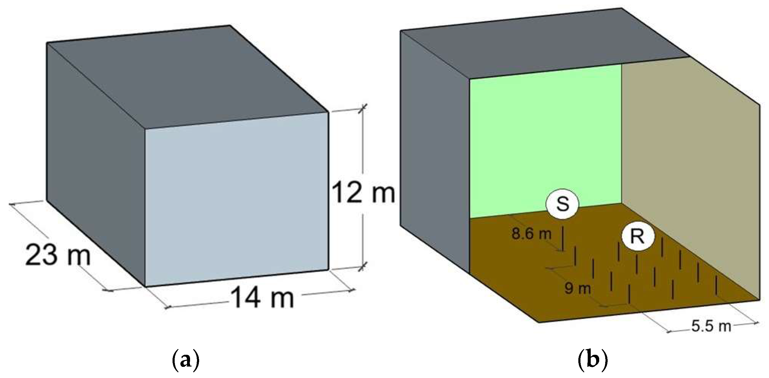
The model room is a theorical space with dimensions similar to a real auditorium without a balcony and with a removed audience slope. The base geometry of the reference auditorium used in the analyses has the following dimensions (see Figure 1), width of 14 m, length of 23 m and height of 12 m, leading to a parallelepiped volume of 3864 m3. The model includes a stage area with dimensions of 9 m by 14 m, and an audience area is also considered with dimensions of 14 m by 14 m. This performance environment is composed of six main surfaces and, in certain cases, the side walls will be divided in two halves to enable the introduction of sound absorption. For each case study, these surfaces will present specific values of sound absorption and dispersion, adapted to the conditions analyzed.
All configurations analyzed have in common the fact that they are based on the volume and stage/audience ratio of a generic auditorium. Sound scattering coefficients usually follow an S-shaped behaviour along the frequency range [30]; however, in the analysis performed in this work, this parameter is assumed to be constant in the frequency domain, and varies in amplitude, ranging from 0.1 to 0.99, for a better understanding of its impact on the reverberation time. As for the sound absorption coefficients, they were also kept constant along the frequency range and, in the following sections, the corresponding amplitudes are defined according to each scenario. An omnidirectional sound source was located at a front position in the stage, corresponding to a distance of 8.6 m from stage back wall and 7 m from the side walls. The acoustic responses were collected at 12 receivers, at 1.5 m high, placed along three lines positioned in the audience area. The room was considered in an unoccupied condition.
The parametric study is performed by isolating different factors, such as analyzing the following:
(i)
Scenarios with different average absorption;
(ii)
The effect of eliminating parallel surfaces;
(iii)
The influence of the volume of the space;
(iv)
The geometrical modelling of a triangular prismatic-shaped diffuser compared to surface modelling using a prescribed sound scattering coefficient.

2.2. Methodology

The simulations presented here were performed using acoustic ray tracing, a geometrical acoustics method that models sound propagation by tracking the paths of rays as they reflect and scatter within an enclosure. An in-house acoustic ray tracing code was used, implemented in MATLAB R2024b [31] (including the Statistics and Machine Learning Toolbox, specifically used for post-processing impulse responses) and executed on a PC running Windows 11, equipped with 64 GB of RAM and an Intel Core i7-14700 processor with a base clock frequency of 2.1 GHz. No GPU-based acceleration was used.
The implementation carried out in this work followed a similar procedure to that employed in previous works by the authors [32,33,34], which proved to be successful in the simulation of a conceptual auditorium and in the prediction of acoustic parameters in a historic environment. Different from the previous publications, in the context of the present paper, the methodology is used to assess a different problem, namely the effect of scattering coefficients and surface irregularity on reverberation time.
The modelling assumption in ray tracing is that the acoustic energy emitted from a sound source can be calculated using an infinite set of acoustic rays, which follow plane wave propagation laws. The energy provided by these rays, which travels in the enclosed space, is decreased by surface absorption or attenuation in the medium and carries no phase information, which is an inherent limitation of the method. The reflected acoustic energy is computed as a combination of a specular component and a scattered component, weighted by the scattering coefficient. In the case of the present analyses, the complete simulation procedure followed a well-defined sequence. First, the room geometry was described by means of several polygons, and the frequency-dependent surface properties (absorption and scattering coefficients) were specified for each polygon. A large number of rays was then emitted uniformly from an omnidirectional (point) source. Each ray was propagated through in straight lines, accounting for air absorption, and interacted with surfaces according to their properties. At every reflection, the energy and reflection direction were updated via surface absorption and the scattering coefficient, and the outgoing direction resulted from the weighted combination of the specular reflection vector and a Lambertian-distributed scattered component. When rays intersected the receiver, their arrival time and remaining energy were recorded for the construction of the room impulse response.
It is particularly relevant to mention that there are several possible implementations to account for the scattering effect at each surface. In the present work the authors adopt a vector mixing approach, for which, at each surface interaction, the outgoing direction is determined by stochastically mixing the specular direction with a scattered direction sampled from a cosine-weighted Lambert distribution [35]. This corresponds to assuming that the angular distribution of the scattered component is independent of the angle of incidence, and that Lambert’s law provides a reasonable approximation for the redistribution of scattered energy [36]. This method preserves the deterministic specular contribution while redistributing only the scattered fraction stochastically, which avoids the over-diffusion associated with fully Lambertian reorientation. Due to the stochastic nature of the algorithm, small run-to-run variations may occur [37,38]. To reduce the influence of this variance, five independent simulations were performed and the averaged results are presented, following common practice in stochastic acoustic ray-tracing, where repeated simulations rapidly reach diminishing variance due to the large number of rays per run.
It should be noted, however, that several authors [18,19] have shown that a vector mixing approach does not always capture the detailed directional characteristics of real diffusive surfaces, particularly for early reflections or source–receiver positions close to the scattering structure. While more advanced models or measured scattering data may increase accuracy in those situations, the aim of this work is not to analyze specific surface types. Therefore, adopting a vector mixing strategy together with averaging over multiple runs is considered adequate for assessing the global influence of sound scattering in the scenarios analyzed herein.
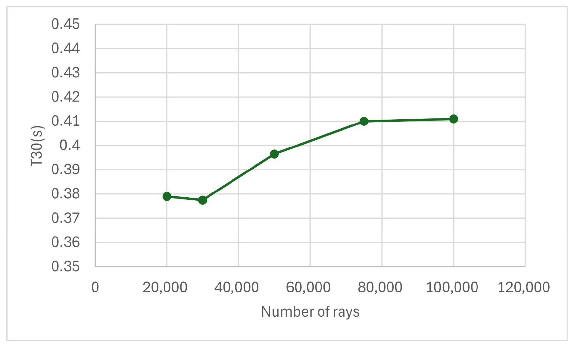
As mentioned, ray tracing modelling uses a large number of rays, emitted by an omnidirectional sound source, covering all incidence angles. The rays travel through the space, losing energy in each reflection according to the sound absorption coefficient of the surfaces [39]. The acoustic response is calculated by a random, finite subset of acoustic ray paths, used as an estimate of the full response. The level of accuracy of the model’s results depends on the number of rays used. If the number of rays is sufficiently large, the simulation results are consistent, whereas too few rays lead to results that may vary significantly between calculations. The number of rays needed depends on the modelled space, including the surface parameters [2]. The number of rays used in the simulations was defined to ensure result stability while maintaining computational efficiency. Based on the statistical error analysis proposed by Vorländer [36] and later by Pelzer et al. [40], relating ray count to absorption area and receiver size, achieving an estimated energy level error below 1 dB for the higher absorption areas considered in this study (606 m2 and 1072 m2) and the receiver radius of 0.1 m would require between 45,000 rays for smaller rooms and 80,000 rays for larger rooms. To verify these assumptions, the effect of ray number in the T30 estimation is illustrated in Figure 2 for the case of the larger room (23 × 14 × 12 m3), with an average sound absorption coefficient of 0.1. For this case, the presented result reveals that a stable result is registered if at least 75,000 rays are used, with an increase to 100,000 rays having an almost negligible effect. The calculation using the approach proposed by Pelzer et al. [40] estimates that 80,000 rays would provide accurate estimations, confirming the observations in the plot.
Following the discussion above, a conservative approach was implemented by using 50,000 rays for smaller volumes and up to 100,000 rays for larger volumes. For the calculation of the room’s impulse responses (IRs), a maximum length of 4.5 s (estimated for the most reverberant space) was considered. Using this computational methodology, it is possible to analyze the IR and calculate, at different locations in the room, several objective acoustic parameters.
Diffuse sound fields may influence some of these parameters; therefore, several investigations have addressed them to obtain a relevant characterization of the acoustic environment. The reverberation time has been the most important parameter when analyzing environments for different types of use, thus focus on this parameter is given in this paper.
The reverberation time (RT) value is determined here from a decrease of 30 dB in the decay curve of the sound pressure level in the room (also referred as T30). The responses were calculated at 12 receivers placed in the audience area, at 500 Hz and 1000 Hz frequency bands, and were then averaged according to the recommendations of the international standard ISO 3382-1 [41]. To assess the perceived differences in the RT and EDT parameters of the room, created by introducing sound scattering in the surfaces, the just noticeable difference (JND) parameter [41] is addressed. The JND values were calculated from the T30 change rate relative to a certain scattering coefficient value, taking the T30 value for the scattering coefficients equal to 0.10 as the reference value as follows:
τ = T 30 ( s = 0.10 ) T 30 ( s ) T 30 ( s = 0.10 ) × 100 %
From the change rate, the #JND (indicating the “number” of JNDs within the variation interval) is obtained by assuming the reference relative threshold of 5% as the significant level, as defined in the ISO 3382-1 [41], meaning that values within 1 #JND are assumed to be perceptually similar. Higher values of the number of #JNDs indicate that the solution will potentially significantly modify the perceived sound quality of the space.

3. Results and Discussion

3.1. Reverberant Scenario

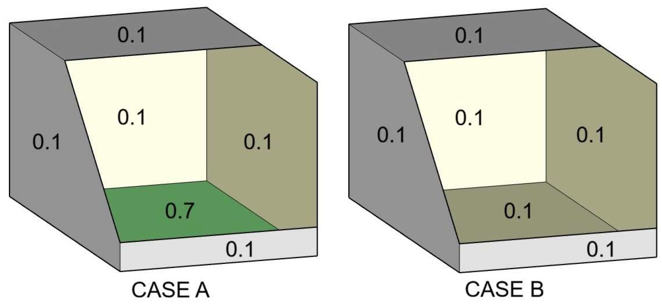
In the first analyzed setup, two situations are considered, as illustrated in Figure 3. Case A has a single sound-absorbent surface, with an absorption coefficient of 0.7, and is located on the floor, while case B has all reflective surfaces with an absorption coefficient corresponding to 0.1. Note that these configurations are theoretical and were defined to reach different reverberation conditions. For both cases, walls and ceilings are reflective, with the floor in case A presenting a sound absorption resembling that provided by upholstered seats with a carpet, while in case B wood seats and floor are being simulated.
The values of the sound absorption coefficient were kept constant at all frequencies, and the sound scattering coefficients (s) of all surfaces varied, with seven simulations performed for each case, increasing values of s from 0.1 to 0.99. Case A presents an average sound absorption coefficient (calculated performing the equivalent sound absorption area divided by the area of the surfaces of the space) of 0.23, while for case B this value is 0.1.

3.1.1. Analysis

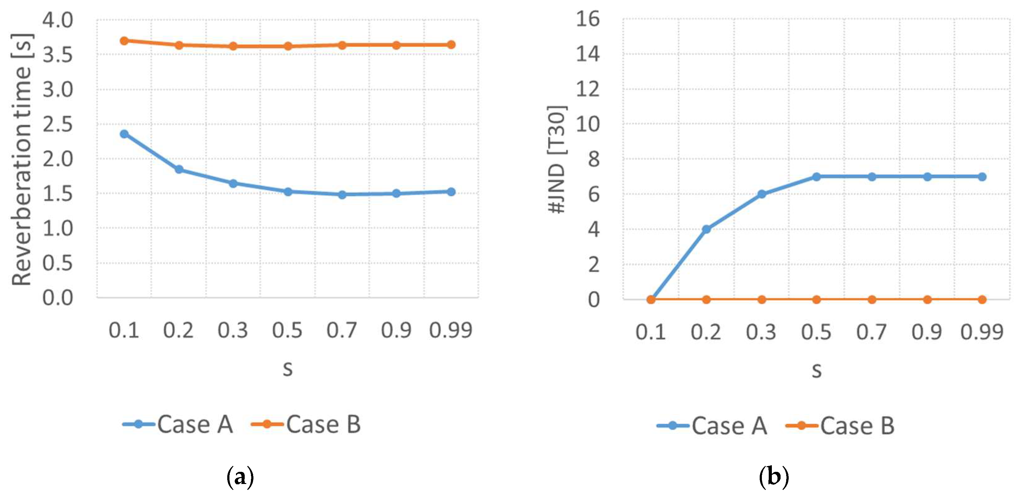
The reverberation times (T30) obtained in both cases are shown in Figure 4a.
In Case A, an increase in the scattering coefficient (s) results in a progressive reduction in the reverberation time, which stabilizes at lower values for s values larger or equal to 0.5. This behaviour is associated with the configuration of the room in Case A, which includes large vertical, reflective and parallel surfaces, combined with a single absorbent surface on the floor. In such an environment, sound energy is primarily reflected between the walls and the ceiling, with only a portion of the reflections reaching the floor. Under these conditions, the introduction of diffusion on the reflective surfaces redirects part of the reflected sound toward the absorbent floor, thereby enhancing energy dissipation and contributing to the observed reduction in T30. These findings are also in accordance with the conclusions provided in [25,26] (where the case studies approach the conditions of the present case) and highlight the critical role of sound scattering in the acoustic optimization of enclosed spaces with parallel reflective surfaces and limited absorption.
In Case B, where all surfaces are reflective and exhibit a uniform sound absorption coefficient of only 0.1, the reverberation time remains high, even as the scattering coefficient increases. This outcome is attributed to the absence of sufficiently absorbent surfaces, which limits the effectiveness of sound scattering in redistributing acoustic energy toward areas capable of dissipating it. Although higher scattering coefficients lead to an increase in the number of diffuse reflections, the sound field continues to be dominated by specular reflections, and the redirected energy ultimately remains within the reflective environment. These results indicate that, in enclosed spaces characterized by parallel reflective surfaces, the implementation of sound diffusers alone is insufficient to significantly modify the T30 parameter. Effective acoustic control in such contexts requires a combined use of scattering and absorption acoustic elements placed in the room.
Regarding the analysis of the #JND [T30], as displayed in Figure 4b, the result for Case A, where the floor is absorbent, shows that the impact of scattering on the reverberation time and the just noticeable difference is high. However, in Case B, where all surfaces are reflective, the change in sound scattering has no perceptible influence on reverberation time, with no #JND variation with the modification of the scattering coefficient.
It is also worth to mention that the standard deviation found for these cases was very low, with a maximum value of 0.05 s registered at s = 0.1 for Case A, and a decreasing tendency for increasing values of the scattering coefficient. These low standard variations mean that there is no significant variation regarding the source to receiver distance or on the distance from the receiver to the diffusive surfaces. In fact, this finding is also in accordance with [26].
To verify the variability of T30 at low scattering coefficients, the sound energy decay curves were obtained for Case A and Case B (the most reverberant environments) for several receivers. Analysis of these curves allowed us to verify that only one slope decay occurs (not displayed here for brevity of the manuscript).
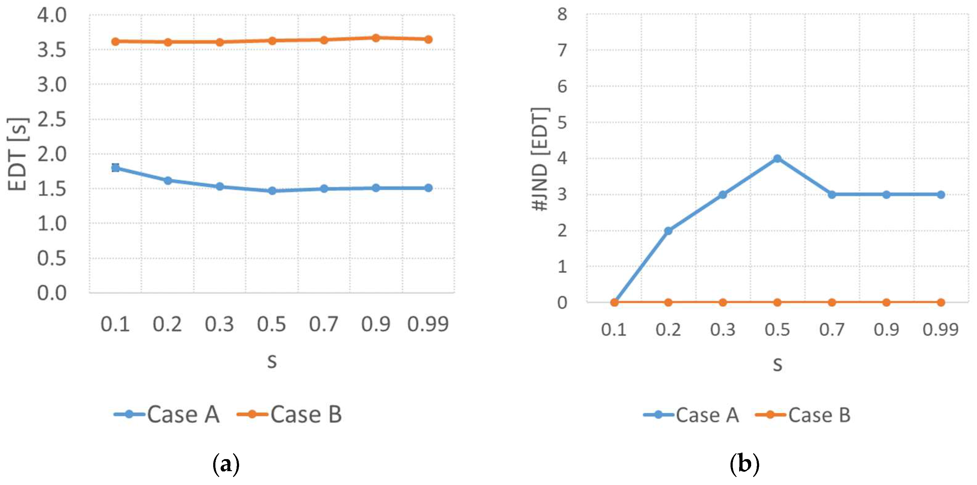
Although the main focus of the work is the T30 parameter, a brief analysis on the impact of scattering in the EDT parameter has been performed. This parameter has been computed as well as the corresponding #JND [EDT] values and results are displayed in Figure 5.
This figure shows that greater #JND values are found for Case A, but they are still quite lower compared to those found for T30. As for Case B, no influence on the contribution of scattering was found.

3.1.2. Summary of Results

To better clarify how scattering interacts in reverberant scenarios, a summary table is provided below (Table 1), highlighting the changes in reverberation time and #JNDs and dominant effects.

3.2. Absorbent Scenario

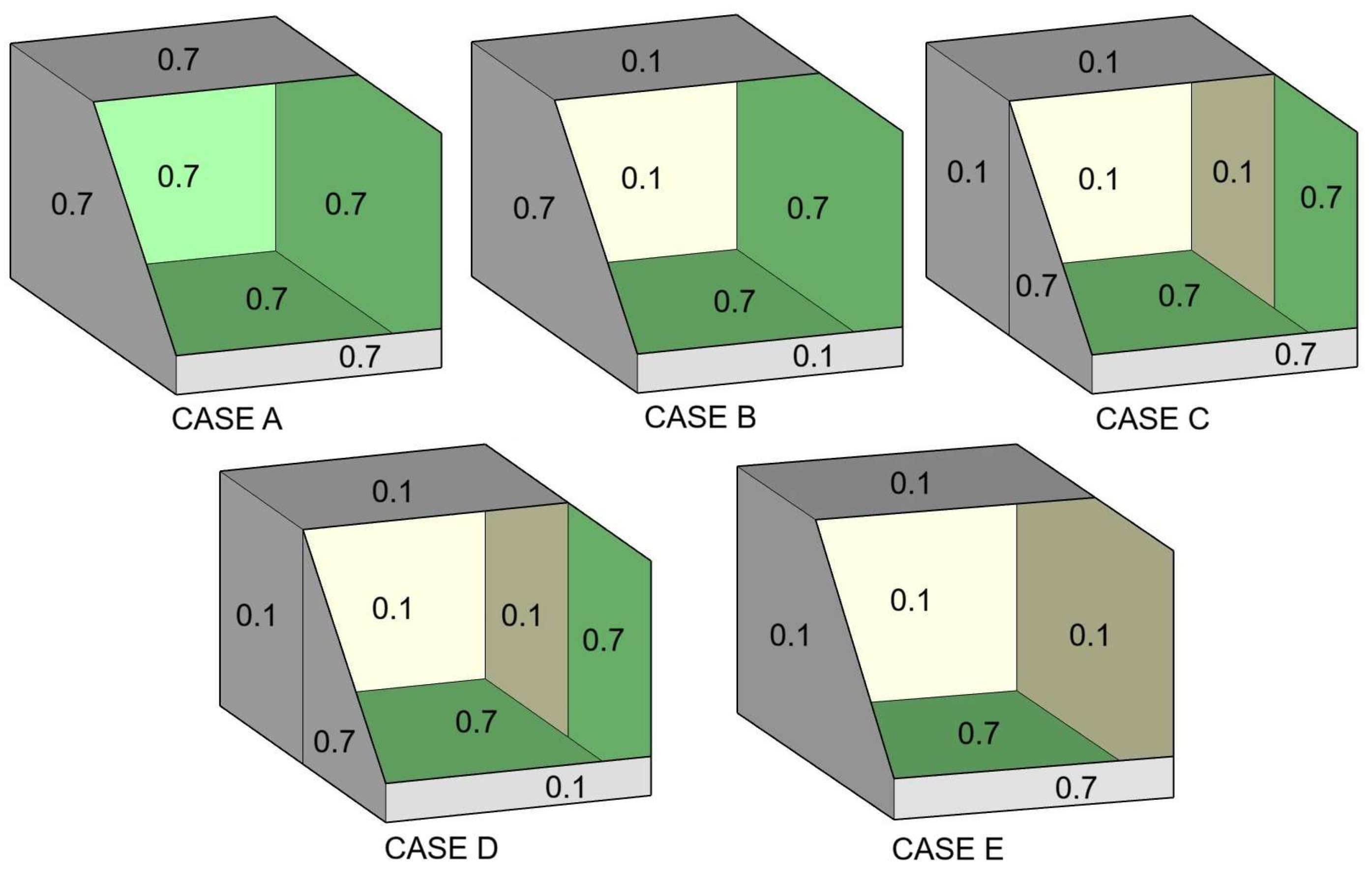
Different configurations were defined to analyze the scenario in which significant sound absorption exists in the room (see Figure 6), in order to evaluate the impact of the location of the sound-absorbent surfaces on the reverberation time (T30). Table 2 shows the average sound absorption coefficients of all the cases analyzed. Case A represents the most absorbent configuration, with a constant sound absorption coefficient of 0.7 on all surfaces. Case B, with an average sound absorption value of 0.44, considers the side walls and the floor as absorbent surfaces. Cases C and D have intermediate average sound absorption coefficients of 0.40 and 0.33, respectively, where the lateral walls were divided into sections with different sound absorption coefficients. Finally, Case E has the lowest average sound absorption of 0.29, where only the floor and the back wall are absorbent, while the other surfaces remain reflective. These changes among cases allow a comparative analysis of the influence of the location and distribution of the sound-absorbent surfaces on acoustic performance in a closed environment.

3.2.1. Analysis

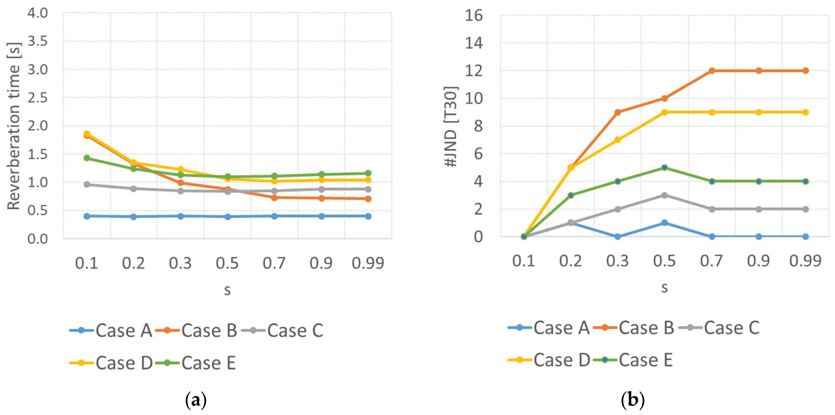
Figure 7a presents the reverberation time for the five analyzed cases as a function of the scattering coefficient. Notice that this coefficient was uniformly applied to all surfaces, increasing from 0.1 to 0.99.
Case A, in which all surfaces have a high sound absorption coefficient (0.7), exhibits the shortest reverberation time among all the cases and shows no significant variation with increasing surface scattering. This behaviour is attributed to the high average absorption, which leads to the immediate attenuation of early reflections. In spaces with high sound absorption, such as in this case, the influence of scattering becomes negligible, as the majority of reflected acoustic energy is rapidly absorbed before it can contribute meaningfully to the sound field.
In the remaining cases, the reverberation time (T30) progressively decreases as the scattering coefficient increases. This trend is due to the lower average sound absorption coefficients in these cases compared to Case A, allowing reflected energy to persist longer within the enclosed space and making the room more responsive to changes in surface scattering.
Comparing Cases B and C, which have similar average absorption coefficients, it is observed that Case B exhibits a more pronounced reduction in T30 with increasing scattering. In this configuration, both the front and back walls are reflective, leading to the formation of floating reflections that contribute to higher reverberation. As the scattering coefficient increases, these reflections are redirected toward absorbent surfaces, resulting in a noticeable decrease in T30. In contrast, Case C includes sound absorption on the back wall, which mitigates the formation of such reflections. As a result, the influence of scattering on the reverberation time is less significant in this case.
Case D, despite having less overall sound absorption, also shows a substantial reduction in T30 with increasing scattering. Similar to Case B, the front and back walls in Case D are reflective and parallel, generating floating reflections that are progressively redirected to absorbent surfaces as scattering increases, thereby reducing reverberation.
Case E, which exhibits the lowest average sound absorption among all configurations, still demonstrates a reduction in T30 as the scattering coefficient increases. This effect is attributed to the presence of reflective lateral walls in the receivers’ zone, which contribute to persistent reflections that are partially mitigated when scattering is introduced.
An analysis of the just noticeable difference (JND) values for these scenarios reveals that Case A presents the lowest #JND values, remaining nearly constant and consistently below or equal to one across all scattering coefficients. This result is not consistent with that provided by [28], who used a uniform absorption coefficient of 0.5 to model a rectangular room and verified that the change rate increased. In Cases C and E, the #JND reaches its peak at a scattering coefficient of 0.5 and then stabilizes at values above 0.7. This suggests that the initial introduction of scattering leads to perceptible changes in T30, but the perceptual impact diminishes with further increase in scattering. In contrast, Cases B and D, which include parallel reflective walls, exhibit the highest #JND values (particularly Case B), indicating that the addition of sound scattering produces pronounced and perceptible changes in reverberation time.
These results imply that, in environments where sound absorption is appropriately distributed (such as in Cases A, C and E), the perceptual impact of scattering on T30 is less significant.
The standard deviation was also evaluated for these cases and a maximum of 0.14 s was calculated, which corresponds to 7.5% from the average value and was registered at s = 0.1 for Case B with a decreasing tendency for increasing values of the scattering coefficient.
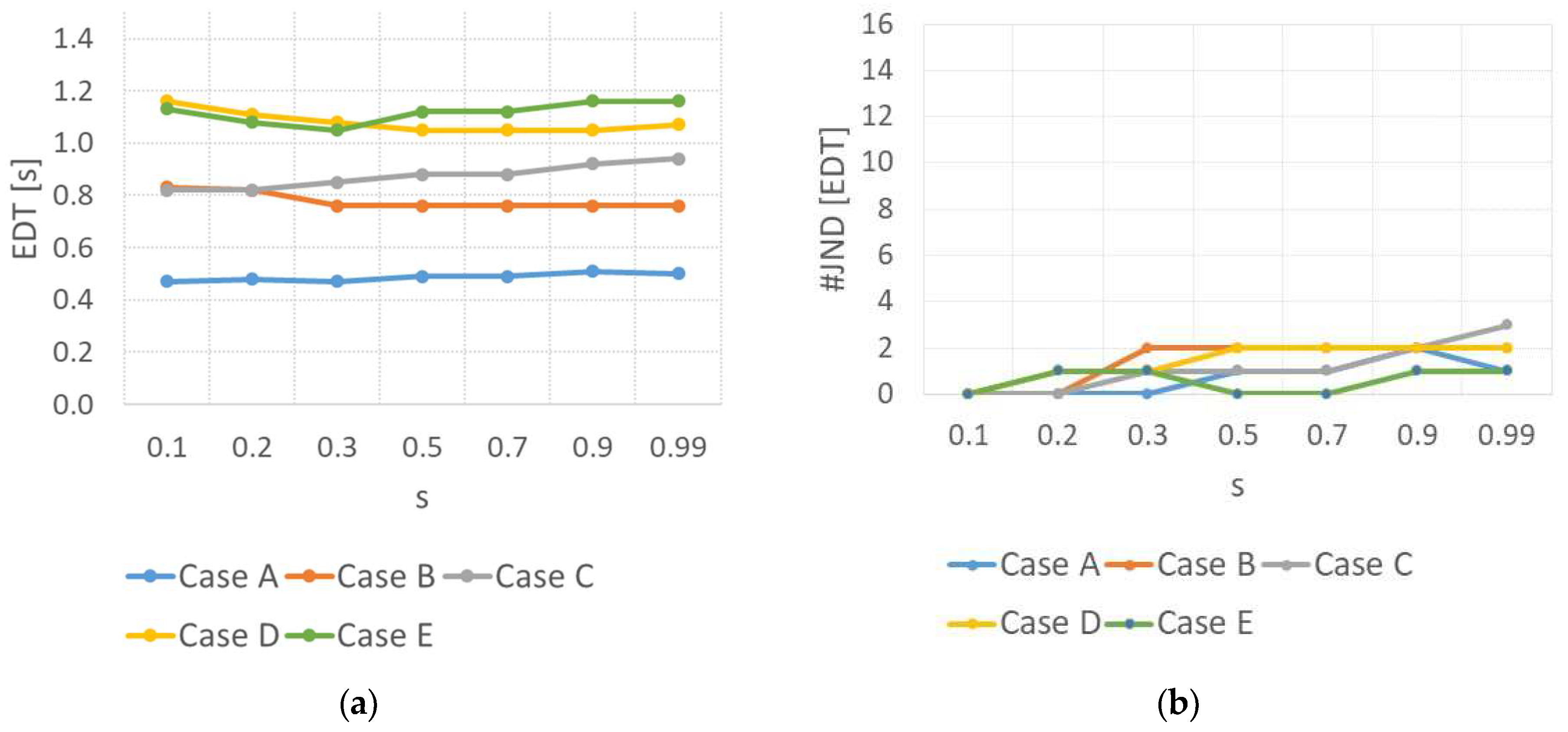
For the second scenario, a brief analysis on the impact of scattering in the EDT parameter was also carried out, and the results are displayed in Figure 8. The plots of this figure evidence smoother curves, almost flat, denoting a different trend from that observed for the reverberation time, the results being little affected by increasing values of scattering. This finding corroborates the conclusions of other works such as Wang [26], where the #JNDs reported for EDT were much smaller than those found for T30.

3.2.2. Summary of Results

In order to support a more systematic comparison among the analyzed absorbent configurations, a synthesis table is presented below (Table 3). This table summarizes the principal characteristics of each case, with particular emphasis on the spatial distribution of sound-absorbing surfaces, average scattering coefficients, effect of scattering on the T30 and #JND values and the main reasons for the observed trends as well as the main conclusions.

3.3. Scenario with Geometric Changes

This section analyses scenarios involving geometric modifications of the enclosed space, specifically by altering the parallelism of the side walls as well as the front and back walls. The objective is to investigate the acoustic impact of these geometric changes on the auditorium acoustics. In particular, the study aims to assess how variations in wall angles influence the behaviour of the reverberation time. In practical design, when employing geometries with non-parallel surfaces, it is important to understand that the contribution of scattering may be a strategy to be employed when the aim is to change the reverberation time. On the other hand, in regular geometries with parallel surfaces, the use of small geometric changes, such as angled surfaces, may have an impact on the reverberation time without requiring any additional cost-effective strategies.
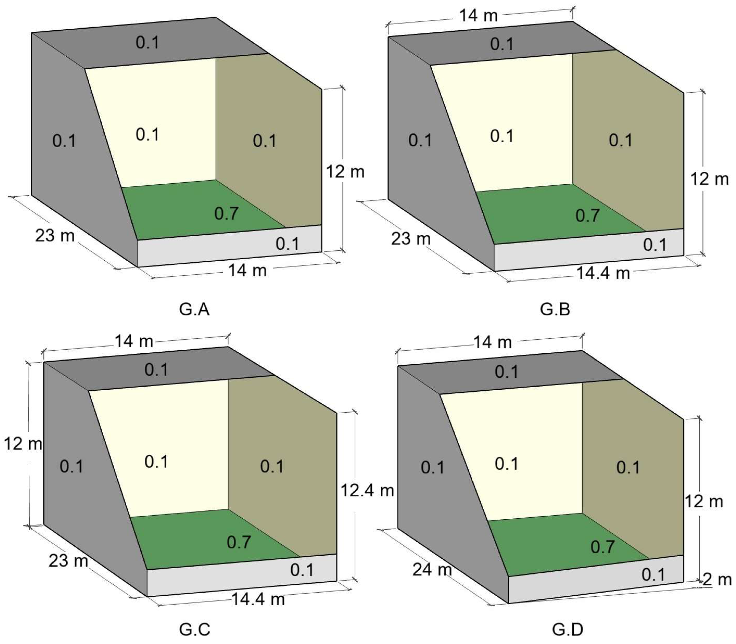
Four cases are studied (eight in total), considering both the reverberant (see Figure 9) and the absorbent scenarios. The values referring to the average sound absorption coefficients and volumes of each case are shown in Table 4 and Table 5.
This approach allows for a more complete assessment of the effects of geometric changes on both a reflective and absorbent space. The G.A Case keeps the dimensions and regular configuration previously analyzed. It is considered as the reference scenario. Case G.B contains a slight increase in the length of the back wall, generating a change in the parallelism of the lateral walls (1-degree angle). In the G.C Case, in addition to the side walls not being parallel, also there is an increase in the back wall height, thus generating a slope (1-degree angle) in the ceiling and modifying the path of the sound reflections. The G.D Case represents the space with a significant increase in the slope of the vertical back wall (8-degree angle, in projection to horizontal plane), resulting in a space with asymmetrical geometry.

3.3.1. Reverberant Setup

The reverberant setup is the first to be analyzed in relation to the changes in the geometry of the space. The G.A Case, with parallel walls, presents the typical acoustic behaviour of a reverberant space with reflective surfaces parallel to each other that generate floating echoes. In the other cases, G.B, G.C and G.D, the modifications in the parallelism of the side walls and in the slope of the ceiling introduce additional reflections, with different directions of propagation, in the closed environment.
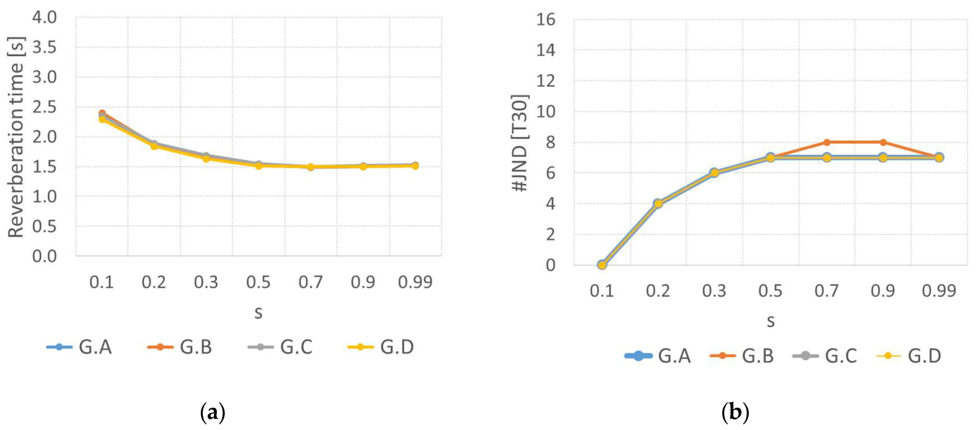
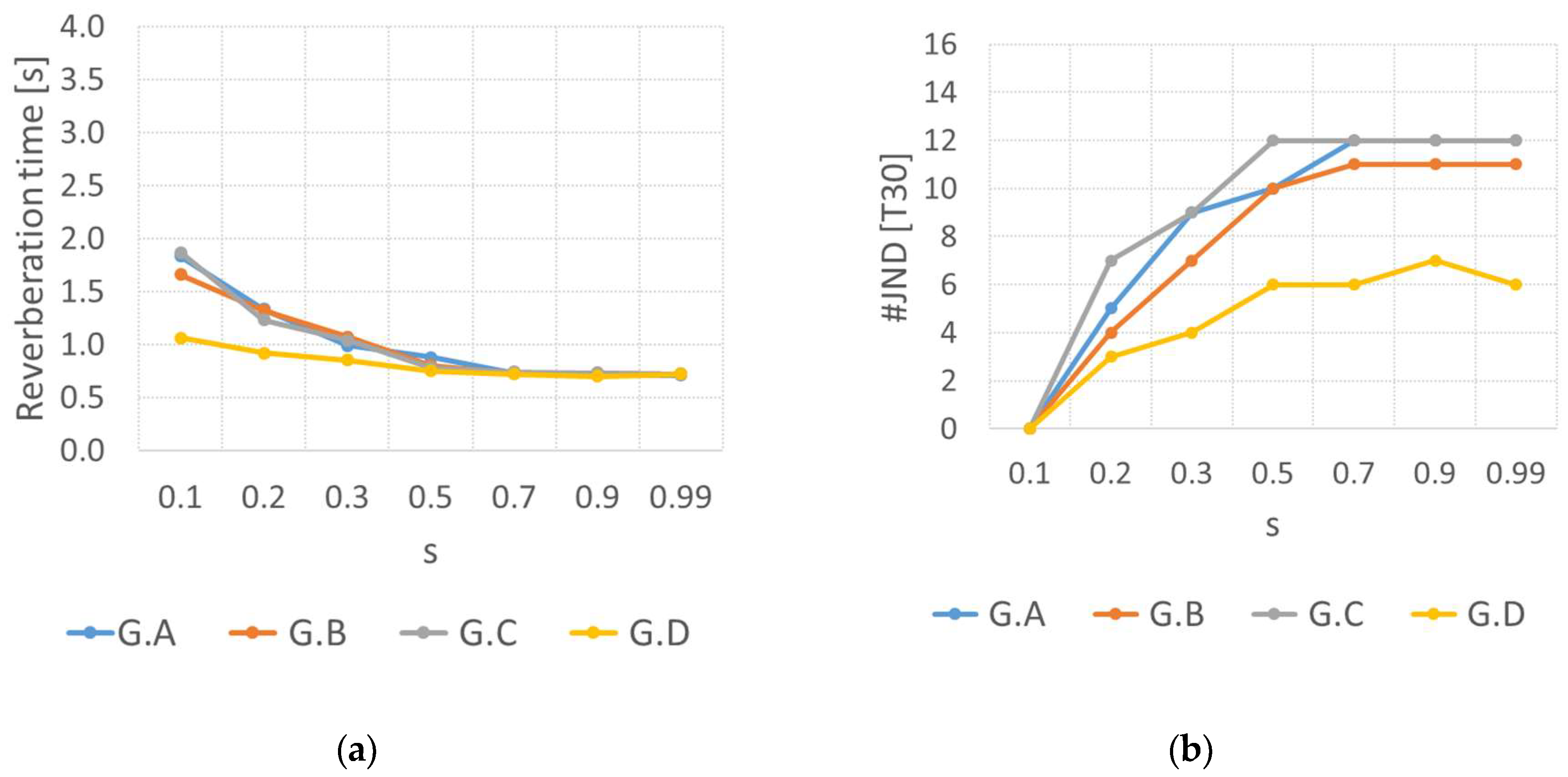
Figure 10 illustrates that all cases, G.A, G.B, G.C, and G.D, show a similar tendency for T30 to decrease as the dispersion coefficient increases. For the lowest value of the scattering coefficient, the highest value of the reverberation time is 2.4 s for all cases. It is also observed that T30 gradually decreases until it stabilizes around 1.5 s from s ≈ 0.5 onwards. However, even with the geometric changes introduced in all cases, there are almost no changes in the acoustic parameter of the room. This behaviour, observed in the reverberant setup, indicates that the absence of absorbent surfaces on the walls or ceiling limits the impact of these changes on the reduction in reverberation time. The gradual reduction in T30 to stabilization around s ≈ 0.5 reinforces that the scattering coefficient plays the main role in the redistribution of sound energy, while geometric changes alone are not enough to substantially modify the reverberation time. This result highlights that the interaction between geometric changes, sound scattering and sound absorption are fundamental for the effective acoustic control of a closed environment.
The analysis of the #JND as a function of the scattering coefficient (see Figure 10b) confirms that the introduction of sound dispersion generates noticeable changes in the environment; however, changes in configurations will not have an impact on the acoustic perception of the closed environment.

3.3.2. Absorbent Setup

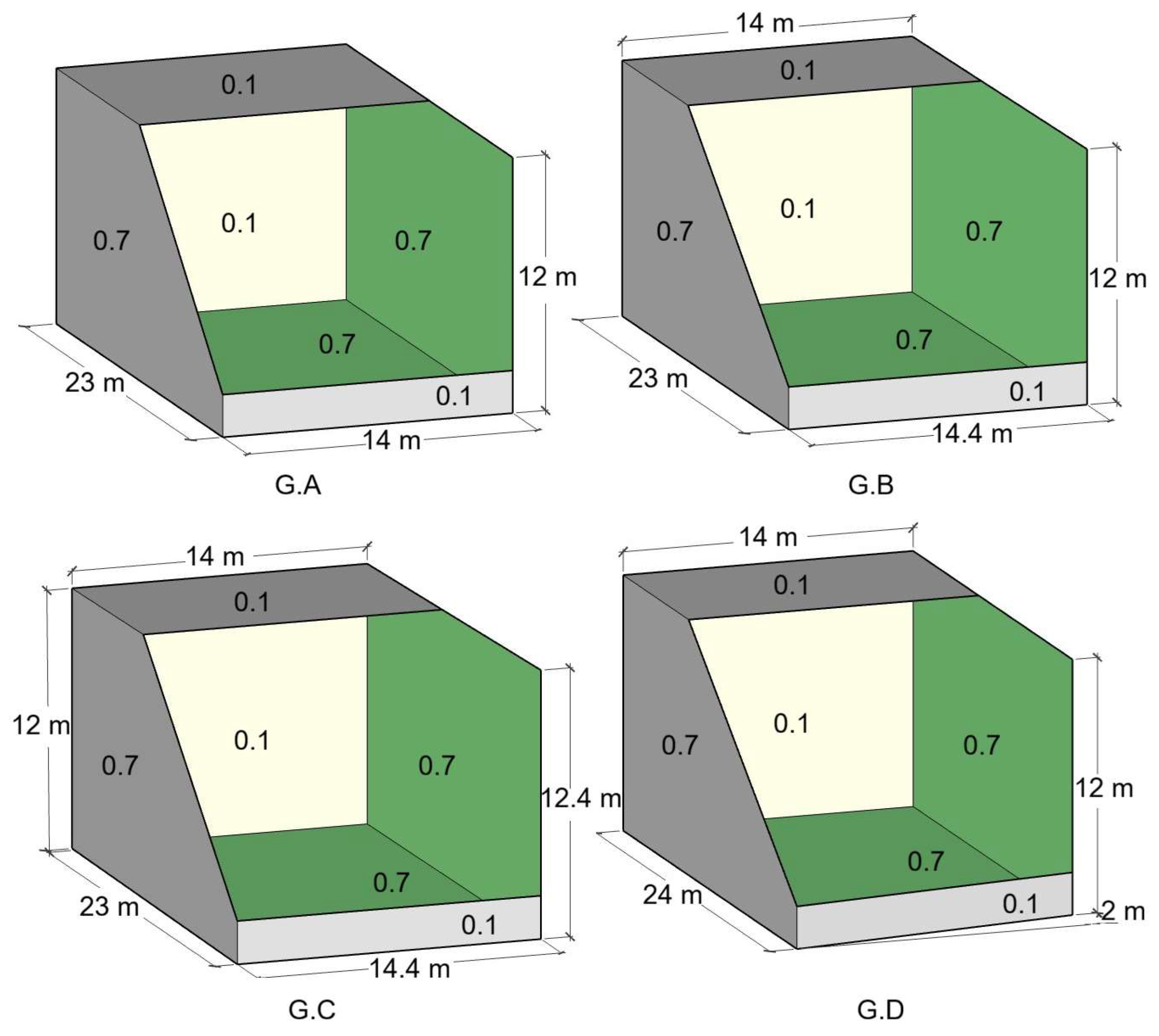
In this section, the same analysis will be carried out for Cases G.A, G.B, G.C and G.D, now considering the absorbent scenario (see Figure 11). An average sound absorption coefficient of 0.44 was selected from the analysis carried out for Case B in the previous section, as it was found to be the most sensitive case to the introduction of sound scattering. This approach will allow a detailed comparison of the effects of geometric changes in a closed environment where surfaces with sound absorption characteristics are prevailing.
Regarding the reverberation time, as seen in Figure 12a, in all cases there is a trend for T30 to decrease as the scattering coefficient (s) increases. Here, Case G.D stands out with the lowest reverberation time, especially at low s values, and provides a lower RT variation with the introduction of sound dispersion. When the parallelism between the front and back walls was removed, the geometric change increased the uniformity in the distribution of sound energy throughout the room, allowing the sound absorption of the surfaces to be more efficient, with the introduction of sound scattering being less effective on the change in the sound field of the closed environment. For the remaining cases (G.B and G.C), the same effect is not perceived, since the surfaces whose slope was changed are absorbent and therefore do not generate multiple reflections.
These results indicate that, in sound-absorbent scenarios, the strategy of introducing geometric changes that remove the parallelism of surfaces plays an important role in the uniformity of the sound field and reduces the need for high sound scattering surfaces to achieve effective reverberation control.
The #JND analysis shown in Figure 12b reveals a clear trend when there is an increase in the scattering coefficient s, thus showing that, even when geometric changes are performed, the introduction of sound dispersion influences sound perception in relation to reverberation time. It is also confirmed that, when parallel surfaces which generate multiple reflections are removed, the need for higher sound dispersion coefficients for the acoustic control of the environment can be reduced. The G.D configuration confirms this observation, presenting a curve with less variation of #JND with increasing sound scattering. These results are consistent with those proposed by Zhu in [28], who modelled a rectangular room with a uniform absorption coefficient of 0.5.

3.3.3. Summary of Results

To support a clearer comparison between the reverberant and absorbent setups, a summary table is presented below (Table 6), highlighting how geometric modifications, such as the presence or absence of parallel reflective surfaces, shape the evolution of the reverberation time and perceptual responses.

3.4. Scenario with Volumetric Changes

Analyzing scenarios related to parallelepiped rooms with volumetric changes makes it possible to investigate the interaction between the volume of the space and the sound scattering coefficients. When the volume of the space increases and the average sound absorption coefficient is kept constant, it is expected that T30 will increase; however, the impact of the sound scattering coefficient on this parameter is not clear.
For this investigation, only the absorbent scenario will be considered. Two different analyses were carried out: in the first, the volumetric change was performed by changing only one dimension of the room (proportional changes) and, in the second, a proportional change in all dimensions (volume scaling) of the room was carried out.

3.4.1. Scenario with Proportional Changes

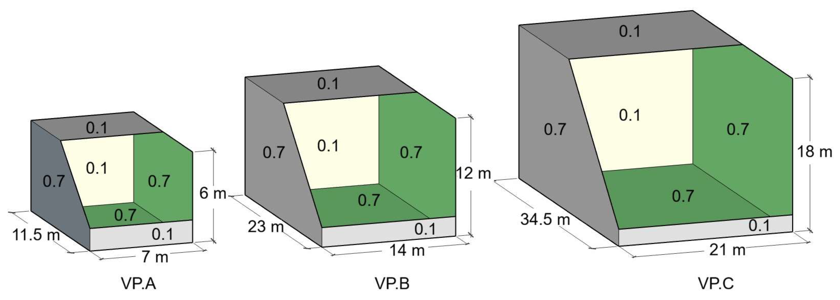
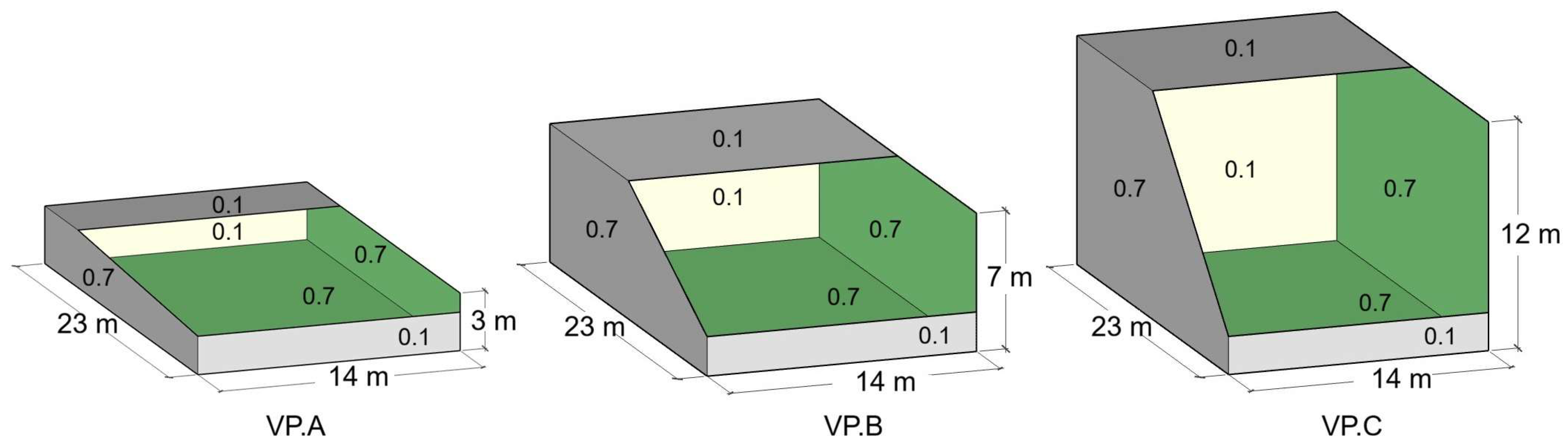
The first analyzed configurations are shown in Figure 13 and the corresponding values of the average sound absorption coefficients and volumes are presented in Table 7. Regarding the dimensional proportions, the VP.C Case, with a volume of 3864 m3, is the reference case (used previously). Case VP.A, with a volume of 966 m3, was obtained from Case VP.C, by only reducing the ceiling height to 3 m. This dimension was chosen because it has the shortest length among all scenarios. The VP.B geometry corresponds to a ceiling height of 7 m, providing a volume of 2252 m3. In these scenarios, the average sound absorption coefficients are very similar.
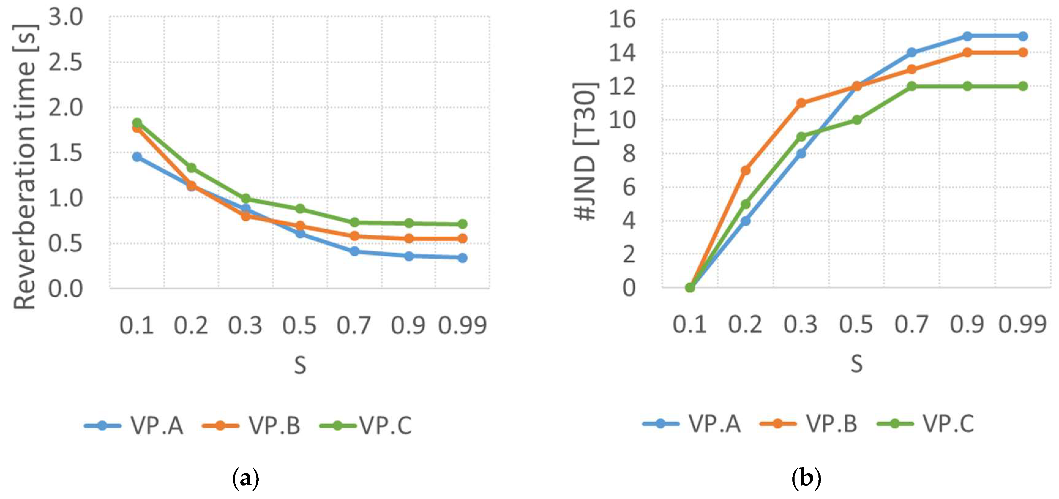
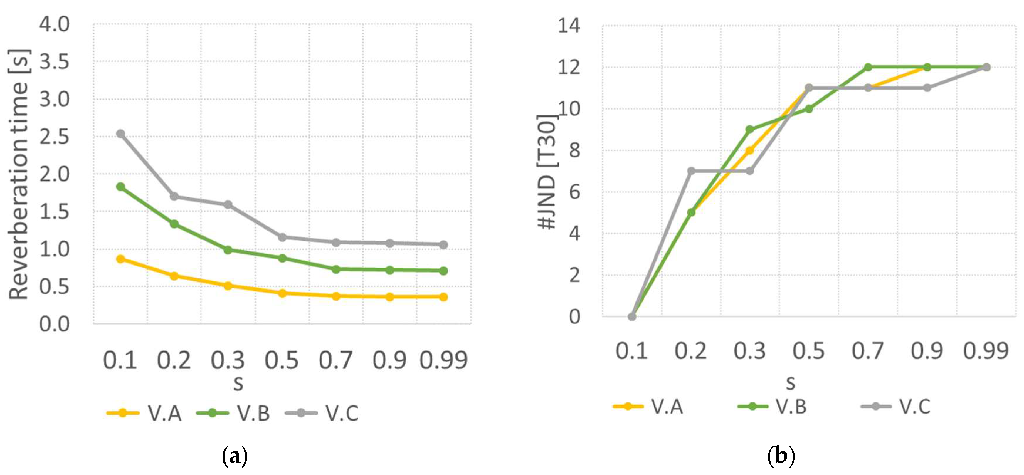
As shown in Figure 14a, the reverberation time shows a trend towards the reduction in this indicator as the sound scattering coefficient increases, and this trend is similar in all cases. As expected, Case VP.C has a higher reverberation time, followed by Case VP.B. However, Case VP.A, with the smallest volume, but also with lower sound absorption, provides a different trend.
When looking into Figure 14b, showing the #JND [T30], there is a marked increase in this parameter in the initial scattering coefficient values for the three cases. From s = 0.7, the values tend to stabilize, suggesting that further increases in dispersion cause less noticeable variations in T30. Among the three cases analyzed, Case VP.A presents higher values from s = 0.7 onwards, meaning that, when sound travels shorter distances, the effect of scattering is more pronounced. Therefore, even small changes in the sound scattering coefficient cause differences in reverberation time, which is reflected in higher #JND values. On the other hand, for Case VP. C, with the highest room height, the #JND values tend to be lower since sound travels longer trajectories between the surfaces, making the reflections more spaced out in time, with the scattering affecting less the perceptible changes in the T30.

3.4.2. Scenario with Volume Scaling

To analyze the effect of a volumetric change when all dimensions are varied proportionally, three cases were considered: Case V.B, with a volume of 3862 m3 (reference case); Case V.C, with a volume of 13,036 m3, obtained from Case V.B by increasing the dimensions 1.5 times; and Case V.A, considering half the dimensions of Case V.B, providing a volume of 482 m3. In all scenarios, the average sound absorption coefficients and their distribution along the surfaces remained constant (see Figure 15 and Table 8).
As illustrated in Figure 16a, the reverberation time also shows a trend towards the reduction in this indicator as the sound scattering coefficient increases, and this trend is similar in all cases. As expected, Case V.C has the highest reverberation time, followed by V.B; Case V.A displays the smallest T30 values due to the decrease in the volume of the room. According to the study by Shtrepi et al. [42], which analysis EDT, the effect of sound scattering becomes more evident as the volume of the room increases, since the sound energy travels longer trajectories before being absorbed; however, this behaviour is not perceived here. In fact, the #JND results (Figure 16b) increase in a similar way for all cases as the function of the scattering coefficient increases.

3.4.3. Summary of Results

To enable a clearer interpretation of the volume transformations explored in this study, the table below (Table 9) summarizes the main acoustic differences observed between proportional height changes (VP) and uniform volume scaling (V).

3.5. Scenario with Geometric Acoustic Diffuser

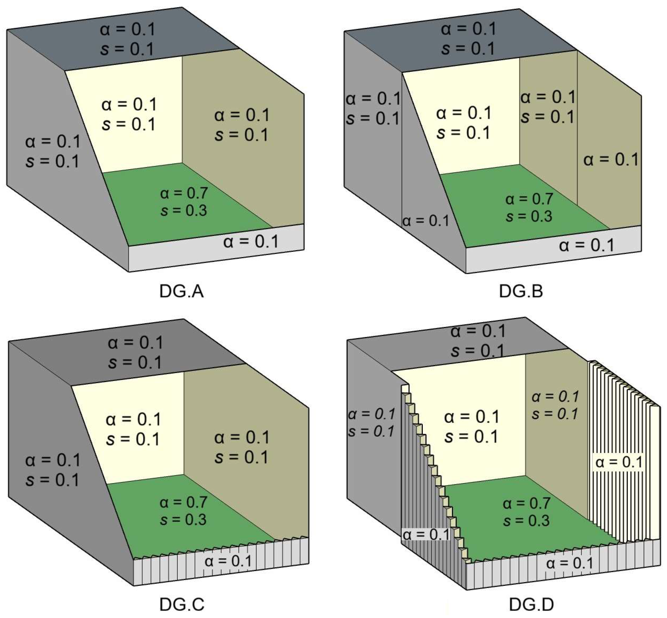
In the acoustic design, the modelling of complex diffusive geometries may be simplified using proper scattering coefficients with similar GA efficiency while decreasing the modelling time. In this section, the modelling level of detail is addressed for a geometric diffuser solution. In this analysis, two reference cases are considered, cases DG.A and DG.B (see Figure 17), to verify the impact on the reverberation time of the geometric shape modelling. In these cases, the scattering was changed only on the surfaces corresponding to the application of the geometric acoustic diffuser. In cases DG.C and DG.D (see Figure 17), diffusers with a triangular prismatic shape, with surfaces 70 cm long, and a sound absorption coefficient of 0.1 are considered. These dimensions were chosen according to references [19,43]. The average sound absorption coefficients and volumes related with all cases are shown in Table 10, presenting very similar values. In the case of DG. C, the geometric diffusers are located at the rear wall of the room, while in the case of DG. D these are placed both on the rear wall and on the back part of the side walls (along 50% of the wall), thus increasing the scattering area.

3.5.1. Analysis

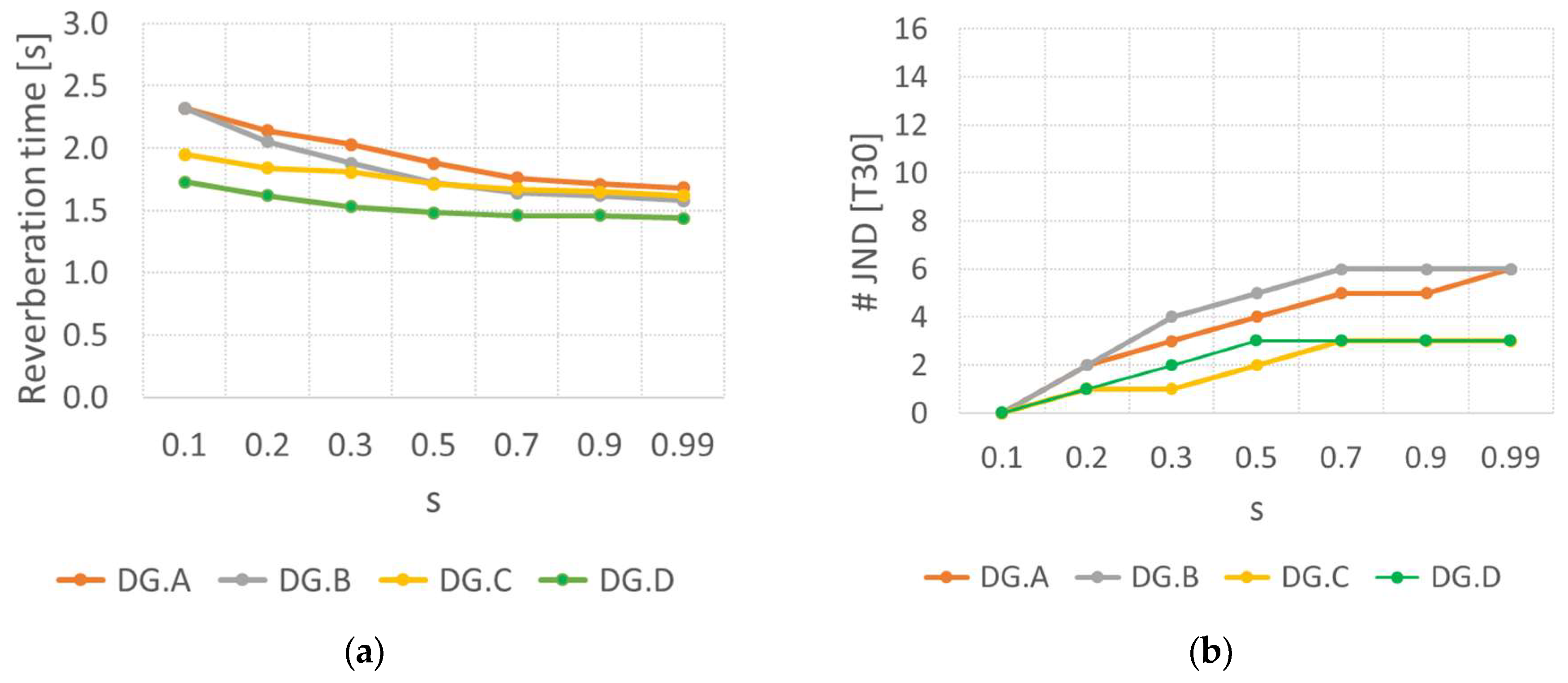
From the analysis of Figure 18a, it can be seen that the reverberation time decreases as the scattering coefficient increases for all scenarios, thus indicating that greater sound dispersion contributes to a more uniform distribution of sound energy throughout the space. The DG.A and DG.B reference cases display higher reverberation times, especially for low values of the scattering coefficient, since the presence of opposite parallel surfaces with reflective properties cannot effectively distribute the sound reflections. Case DG.C has a lower reverberation time compared to Case DG.A, the reference case, revealing that the acoustic diffusers in the back part of the room help to redistribute the sound in the environment without introducing significant sound absorption. This results in a more uniform dispersion of sound. Case DG.D has the lowest reverberation time, although the acoustic diffusers display reflective surfaces. The distribution of the acoustic diffusers on the side and back walls allows the sound to be significantly redirected, reducing the concentration of sound energy in certain areas and, consequently, reducing the reverberation time. From the analysis of Figure 18a, it is also observed that the reverberation time of prismatic acoustic diffuser cases (DG.C and DG.D) for lower values of the scattering coefficient (such as 0.1) can already approach the performance of cases where the surface is flat (DG.A and DG.B) when the scattering coefficient is assumed to be 0.5. This indicates that an acoustic behaviour similar to that of the prismatic geometry can be achieved by modelling a smooth surface, assuming a scattering coefficient of 0.5. This result is in accordance with that provided by [19].
Regarding the analysis of the #JND, which is plotted in Figure 18b, cases DG.A and DG.B have the highest #JNDs, indicating that the introduction of sound dispersion on smooth surfaces provides noticeable changes in reverberation. It is also visible that Case DG.B introduces larger amplitudes than Case DG.A, as a larger surface area with diffusing properties was introduced. Case DG.C shows lower values of the #JND, suggesting that the prismatic diffusion geometry located in the back, in spite of being reflective, helps to distribute the sound, which makes the changes associated with the presence of scattering smaller. Case DG.D also provides low #JND values, highlighting this behaviour. It can be concluded that balanced sound scattering avoids acoustic problems, such as flutter echoes, and creates a more homogeneous perception of the closed space.

3.5.2. Summary of the Results

To clarify the distinct acoustic roles played by modelling scattering, the table below (Table 11) provides a comparative summary of configurations employing flat reflective surfaces versus geometric diffusers.

4. Conclusions

In the present paper, the influence of sound scattering on the acoustic performance of a theoretical shoebox-shaped room has been addressed, using ray-tracing simulations, where scattering by the surfaces was assumed by means of a vector mixing approach. A systematic parametric analysis was performed, focusing on the reverberation time (T30) and its perceptual relevance by means of #JND, regarding the effect of the following: sound absorption of the room, eliminating parallel surfaces through surfaces inclination, changes in room volume of the space and proportions or the geometrical modelling of a triangular prismatic-shape diffuser.
The results demonstrated that the introduction of sound scattering is efficient in the redistribution of acoustic energy, enabling reductions in reverberation time in rooms with parallel surfaces that tend to generate floating reflections, provided that sufficient and well-distributed absorption is present. In highly reverberant rooms, increasing scattering alone is inefficient, so absorption must be established as a primary design strategy before scattering can yield meaningful benefits. Additionally, geometric modifications, achieved by introducing non-parallel (angled) surfaces, have shown to be particularly effective in mitigating floating reflections and reducing the dependence of scattering. From a practical design perspective, such geometric solutions should be prioritized as a robust and cost-effective means of improving acoustic quality. In rooms employing non-parallel surfaces, the contribution of additional surface scattering to reverberation control becomes less significant.
The analysis carried out with respect to volume scaling suggests that the perceptual impact of scattering on the reverberation time is negligible. However, modifications to the room’s dimensional proportions exert a stronger effect on the perception of reverberation, suggesting that scattering is more effective in geometries where one dimension is significantly lower than the remaining ones when increasing scattering. This finding highlights the importance of considering room proportions, rather than volume alone, when employing scattering as a design or modelling parameter.
Finally, it was also found from the geometric modelling of prismatic diffusers that this shape provided efficient sound scattering. producing an acoustic behaviour comparable to that obtained with flat surfaces assigned with medium scattering coefficients. This result has practical implications for acoustic modelling, indicating that these complex diffusive geometries may be simplified using flat surfaces with proper surface scattering coefficients, thereby decreasing modelling complexity and computation time.
Finally, the study has several limitations that should be acknowledged. The results presented here were not compared with experimental measurements, and therefore the conclusions are valid in the context of computational simulation algorithms for room acoustics. Moreover, the ray-tracing approach used here is an energy-based, high-frequency approximation that neglects wave-related phenomena such as diffraction and interference, which limits its validity at low frequencies. Although material properties are inherently frequency-dependent, the analysis was restricted to the 500 Hz and 1000 Hz octave bands, as these mid-frequencies fall within the reliable operating range of geometrical acoustics and are widely used as reference bands for assessing room behaviour. Additionally, the simulations considered frequency-independent scattering coefficients and focused solely on reverberation time metrics. Future research should extend this work by incorporating frequency-dependent scattering, additional acoustic parameters, different geometries, early reflection behaviour, and experimental validation to further refine the understanding of scattering effects in room acoustics.


Author Contributions

Conceptualization, A.P.; methodology, A.P.; software, A.G. and L.G.; formal analysis, A.P. and D.M.; investigation, A.P. and L.G.; writing—original draft preparation, A.P. and P.A.-M.; writing—review and editing—P.A.-M.; visualization, A.G.; supervision, A.P.; funding acquisition, L.G. All authors have read and agreed to the published version of the manuscript.

Funding

This work was supported by the Fundação para a Ciência e a Tecnologia (FCT) through national funds and by the Fundo Europeu de Desenvolvimento Regional (FEDER) through the Thematic Programme Innovation and Digital Transition (COMPETE 2030), under Portugal 2030, and by the European Union, within the framework of Project No. 14677 | COMPETE2030-FEDER-00917500 (https://doi.org/10.54499/2023.16029.ICDT). This work was also supported by FCT/MCTES under the R&D Unit Institute for Sustainability and Innovation in Structural Engineering (ISISE), under the references UID/4029/2025 (https://doi.org/10.54499/UID/04029/2025) and UID/PRR/04029/2025 (https://doi.org/10.54499/UID/PRR/04029/2025), and under the Associate Laboratory Advanced Production and Intelligent Systems ARISE under reference LA/P/0112/2020.

Data Availability Statement

The raw data supporting the conclusions of this article will be made available by the authors on request.

Conflicts of Interest

The authors declare no conflicts of interest.

References

  1. Barron, M. Acoustics for multi-purpose use. In Auditorium Acoustics and Architectural Design, 2nd ed.; Spon Press: London, UK; New York, NY, USA, 2010; pp. 385–408. [Google Scholar]
  2. Cox, T.; d’Antonio, P. Acoustic Absorbers and Diffusers: Theory, Design and Application, 3rd ed.; CRC Press: London, UK; New York, NY, USA, 2017. [Google Scholar]
  3. Carrión Isbert, A. Diseño Acústico de Espacios Arquitectónicos; Univ. Politèc. de Catalunya: Barcelona, Spain, 1998. [Google Scholar]
  4. Haan, C.H.; Fricke, F.R. An evaluation of the importance of surface diffusivity in concert halls. Appl. Acoust. 1997, 51, 53–69. [Google Scholar] [CrossRef]
  5. Nolan, M.; Berzborn, M.; Fernandez-Grande, E. Isotropy in decaying reverberant sound fields. J. Acoust. Soc. Am. 2020, 148, 1077–1088. [Google Scholar] [CrossRef]
  6. Nilsson, E.; Arvidsson, E. An Energy Model for the Calculation of Room Acoustic Parameters in Rectangular Rooms with Absorbent Ceilings. Appl. Sci. 2021, 11, 6607. [Google Scholar] [CrossRef]
  7. MBerzborn, M. Vorländer Directional sound field decay analysis in performance spaces. Build. Acoust. 2021, 28, 249–263. [Google Scholar] [CrossRef]
  8. Xie, D.; Wittebol, W.; Li, Q.; Maarten, H. A method for extracting an average scattering coefficient for room acoustic modeling. Appl. Acoust. 2025, 233, 110604. [Google Scholar] [CrossRef]
  9. ISO 17497-1; Acoustics—Measurement of Sound Scattering Properties of Surfaces. Part 1: Measurement of the Random-Incidence Scattering Coefficient in a Reverberation Room. International Organization for Standardization: Geneva, Switzerland, 2004.
  10. ISO 17497-2; Acoustics—Sound-Scattering Properties of Surfaces. Part 2: Measurement of the Directional Diffusion Coefficient in a Free Field. International Organization for Standardization: Geneva, Switzerland, 2012.
  11. Vorländer, M.; Mommertz, E. Definition and measurement of random incidence scattering coefficients. Appl. Acoust. 2000, 60, 187–199. [Google Scholar] [CrossRef]
  12. Cox, T.; Dalenbäck, B.; D’Antonio, P.; Embrechts, J.; Jeon, J.; Mommertz, E.; Vorländer, M. A tutorial on scattering and diffusion coefficients for room acoustic surfaces. Acust. Acta Acust. 2006, 92, 1–15. [Google Scholar]
  13. Lam, Y.W. A comparison of three diffuse reflection modeling methods used in room acoustics computer models. J. Acoust. Soc. Am. 1996, 100, 2181–2192. [Google Scholar] [CrossRef]
  14. Bork, I. A comparison of room simulation software—The 2nd round robin on room acoustical computer simulation. Acust. Acta Acust. 2000, 86, 943–956. [Google Scholar]
  15. Vorländer, M. Computer simulations in room acoustics: Concepts and uncertainties. J. Acoust. Soc. Am. 2013, 133, 1203–1213. [Google Scholar] [CrossRef] [PubMed]
  16. Savioja, L.; Svensson, P. Overview of geometrical room acoustic modeling techniques. J. Acoust. Soc. Am. 2015, 138, 708–730. [Google Scholar] [CrossRef] [PubMed]
  17. Autio, H.; Vardaxis, N.-G.; Hagberg, D.B. The Influence of Different Scattering Algorithms on Room Acoustic Simulations in Rectangular Rooms. Buildings 2021, 11, 414. [Google Scholar] [CrossRef]
  18. Shtrepi, L.; Astolfi, A.; Puglisi, G.E.; Masoero, M.C. Effects of the Distance from a Diffusive Surface on the Objective and Perceptual Evaluation of the Sound Field in a Small Simulated Variable-Acoustics Hall. Appl. Sci. 2017, 7, 224. [Google Scholar] [CrossRef]
  19. Shtrepi, L. Investigation on the diffusive surface modeling detail in geometrical acoustics based simulations. J. Acoust. Soc. Am. 2019, 145, EL215–EL221. [Google Scholar] [CrossRef]
  20. Suzumura, Y.; Sakurai, M.; Ando, Y.; Yamamoto, I.; Iizuka, T.; Oowaki, M. An evaluation of the effects of scattered reflections in a sound field. J. Sound Vib. 2000, 232, 303–308. [Google Scholar] [CrossRef]
  21. Chiles, S.; Barron, M. Sound level distribution and scatter in proportionate spaces. J. Acoust. Soc. Am. 2004, 116, 1585–1595. [Google Scholar] [CrossRef]
  22. Ryu, J.K.; Jeon, J.Y. Subjective and objective evaluations of a scattered sound field in a scale model opera house. J. Acoust. Soc. Am. 2008, 124, 1538–1549. [Google Scholar] [CrossRef]
  23. Kim, Y.H.; Kim, J.H.; Jeon, J.Y. Scale model investigations of diffuser application strategies for acoustical design of performance venues. Acust. Acta Acust. 2011, 97, 791–799. [Google Scholar] [CrossRef]
  24. Lam, Y.W. The dependence of diffusion parameters in a room acoustics prediction model on auditorium sizes and shapes. J. Acoust. Soc. Am. 1996, 100, 2193–2203. [Google Scholar] [CrossRef]
  25. Wang, L.; Rathsam, J. The influence of absorption factors on the sensitivity of a virtual room’s sound field to scattering coefficients. Appl. Acoust. 2008, 69, 1249–1257. [Google Scholar] [CrossRef]
  26. Shtrepi, L.; Astolfi, A.; Pelzer, S.; Vitale, R.; Rychtáriková, M. Objective and perceptual assessment of the scattered sound field in a simulated concert hall. J. Acoust. Soc. Am. 2015, 138, 1485–1497. [Google Scholar] [CrossRef] [PubMed]
  27. Mateus, D.; Pereira, A. Proposal of a simplified methodology for reverberation time prediction in standard medium size rooms with non-uniformly distributed sound absorption. Acta Acust. 2023, 7, 31. [Google Scholar] [CrossRef]
  28. Zhu, X.; Kang, J.; Ma, H. The Impact of Surface Scattering on Reverberation Time in Differently Shaped Spaces. Appl. Sci. 2020, 10, 4880. [Google Scholar] [CrossRef]
  29. Zhu, X.; Xu, G.; Kang, J.; Xue, X.; Hao, Y. Influence of Surface Scattering on Auditorium Acoustic Parameters. Buildings 2024, 14, 1882. [Google Scholar] [CrossRef]
  30. Vorländer, M.; Feistel, S. Show your scattering coefficients. Proc. Meet. Acoust. 2022, 50, 015003. [Google Scholar] [CrossRef]
  31. The MathWorks, Inc. MATLAB, version R2024b; The MathWorks, Inc.: Natick, MA, USA, 2024.
  32. Pereira, A.; Gaspar, A.; Godinho, L.; Amado-Mendes, P.; Mateus, D.; Carbajo, J.; Ramis, J.; Poveda, P. On the use of Perforated sound absorption systems for variable acoustics room design. Buildings 2021, 11, 543. [Google Scholar] [CrossRef]
  33. Carbajo, J.; Poveda-Martínez, P.; Godinho, L.; Pereira, A.; Gaspar, A.; Amado-Mendes, P.; Mateus, D.; Ramis, J. Tunable Perforated Panel Sound Absorbers for Variable Acoustics Room Design. Appl. Sci. 2024, 14, 2094. [Google Scholar] [CrossRef]
  34. Amado Mendes, P.; Godinho, L.; Mateus, D.; Pereira, A.; Ramos, D.; Gaspar, A. Analysis of the reconstructed acoustic environment of a Portuguese romanesque cathedral in the 16th century by numerical modelling. In Proceedings of the Forum Acusticum Euronoise 2025, Málaga, Spain, 23–26 June 2025; European Acoustics Association: Madrid, Spain, 2025. [Google Scholar] [CrossRef]
  35. Kuttruff, H. Room Acoustics, 4th ed.; Spon Press: New York, NY, USA, 2000. [Google Scholar]
  36. Vorländer, M. Auralization: Fundamentals of Acoustics, Modeling, Simulation, Algorithms and Acoustic Virtual Reality; Springer: Berlin, Germany, 2008. [Google Scholar]
  37. Dalenbäck, B. Engineering principles and techniques in room acoustics prediction. In Proceedings of the Baltic-Nordic. Acoustics Meeting, Bergen, Norway, 10–12 May 2010; Available online: http://www.catt.se/BNAM-Bergen-2010-CATT.pdf (accessed on 15 December 2025).
  38. Postma, B.; Katz Brian, F.G. Creation and calibration method of acoustical models for historic virtual reality auralizations. Virtual Real. 2015, 19, 161–180. [Google Scholar] [CrossRef]
  39. Rindel, J.H. The use of computer modelling in room acoustics. J. Vibroengineering 2000, 3, 219–224. [Google Scholar]
  40. Pelzer, S.; Schröder, D.; Vorlaender, M. The number of necessary rays in geometrically based simulations using the diffuse rain technique. In Proceedings of the DAGA, Düsseldorf, Germany, 21–24 March 2011. [Google Scholar]
  41. ISO 3382-1:2009; Acoustics—Measurement of Room Acoustic Parameters—Part 1: Performance Spaces. International Organization for Standardization: Brussels, Belgium, 2009.
  42. Shtrepi, L.; Astolfi, A.; Rychtáriková, M. The influence of a volume scale-factor on scattering coefficient effects in room acoustics. Build. Acoust. 2014, 21, 153–166. [Google Scholar] [CrossRef]
  43. Available online: https://www.rpgeurope.com/products/product/triffusor.html (accessed on 5 March 2025).
Figure 1. Geometry of the shoebox room considered as reference: (a) definition of external dimensions; (b) definition of the location of the sound source (S) and receivers’ positions (R).
Applsci 16 01960 g001
Figure 2. Variation in T30 with the number of emitted rays for the case of a room with dimensions 23 × 14 × 12 m3, and an absorption coefficient of 0.1.
Applsci 16 01960 g002
Figure 3. Overview of the scenario with a reverberant room, indicating the respective sound absorption coefficients considered for each surface: Case A, with reflective walls and ceiling (α = 0.1) and absorbing floor (α = 0.7); Case B, with all surfaces reflective (α = 0.1).
Applsci 16 01960 g003
Figure 4. Results regarding the simulation of the reverberant scenario, where (a) is the reverberation time and (b) corresponds to #JND [T30].
Applsci 16 01960 g004
Figure 5. Results regarding the simulation of the reverberant scenario, where (a) is the early decay time (EDT) and (b) corresponds to #JND [EDT].
Applsci 16 01960 g005
Figure 6. Illustration of the different cases considered for the absorbent scenario, indicating the sound absorption coefficient (α) attributed to each surface. Progressively decreasing levels of sound absorption are considered when moving from Case A (all surfaces with α = 0.7) to Case E (all surfaces with α = 0.1, and only the floor with α = 0.7).
Applsci 16 01960 g006
Figure 7. Results regarding the simulation of the absorbent scenario, where (a) is the reverberation time and (b) corresponds to #JND [T30] analysis.
Applsci 16 01960 g007
Figure 8. Results regarding the simulation of the absorbent scenario, where (a) is the early decay time and (b) corresponds to #JND [EDT].
Applsci 16 01960 g008
Figure 9. Illustration of the different cases considered for the scenario with geometric changes; all cases consider walls and ceiling with α = 0.1 and the floor with α = 0.7 (reverberant setup): Case G.A, with a parallelepiped room; Case G.B, introducing a small increase in width towards the back of the room (increasing from 14.0 m to 14.4 m); Case G.C, considering both an increase in width (14.0 m to 14.4 m) and height (12.0 m to 12.4 m) towards the back of the room; Case G.D, assuming that the back wall is not parallel to the front wall.
Applsci 16 01960 g009
Figure 10. Results regarding simulation of the scenarios with geometric changes, considering the reverberant setup, where (a) is the reverberation time and (b) corresponds to #JND [T30].
Applsci 16 01960 g010
Figure 11. Illustration of the different cases considered for the scenario with geometric changes; all cases consider side walls and floor with α = 0.7, and the back and front walls and ceiling with α = 0.1 (absorbent setup): Case G.A assumes a parallelepiped room is considered; Case G.B introduces a small increase in width towards the back of the room (increasing from 14.0 m to 14.4 m); Case G.C considers both an increase in width (14.0 m to 14.4 m) and height (12.0 m to 12.4 m) towards the back of the room; Case G.D assumes that the back wall is not parallel to the front wall.
Applsci 16 01960 g011
Figure 12. Results regarding the simulation of the scenarios with geometric changes, considering the absorbent space, where (a) is the reverberation time and (b) corresponds to #JND [T30].
Applsci 16 01960 g012
Figure 13. Illustration of the scenario with volumetric changes by modification of the room height: VP.A, with height 3.0 m; VP.B, with height 7.0 m; VP.C, with height 12.0 m.
Applsci 16 01960 g013
Figure 14. Results regarding the simulation of the scenarios with volumetric changes by changing room height, where (a) is the reverberation time and (b) corresponds to #JND [T30].
Applsci 16 01960 g014
Figure 15. Illustration of the scenario with volumetric changes, by proportionally varying all room dimensions: VP.A, with a volume of 483 m3; VP.B, with a volume of 3864 m3; VP.A, with a volume of 13,041 m3.
Applsci 16 01960 g015
Figure 16. Results regarding the simulation of the scenario with volumetric changes, by proportionally varying all room dimensions, where (a) is the reverberation time and (b) corresponds to #JND [T30].
Applsci 16 01960 g016
Figure 17. Illustration of the scenarios in which the geometric acoustic diffusive surface is effectively modelled: DG.A (allowing the scattering coefficient to vary in the back part in the back wall) and DG.B (allowing the scattering coefficient to vary in the back part of the lateral walls and in the back wall) are reference cases with flat surfaces; DG.C and DG.D correspond to the same cases but different modelling of the geometry of the diffuser. Fixed scattering and absorption coefficients are indicated at each surface.
Applsci 16 01960 g017
Figure 18. Results regarding the simulation of the scenarios with geometrical acoustic diffusers, where (a) is the reverberation time (T30) and (b) corresponds to #JND [T30].
Applsci 16 01960 g018
Table 1. Summary of results for the reverberant scenario.
AspectCase ACase B
Surface Absorption SetupFloor is absorbent ( α = 0.7 ); walls & ceiling reflective ( α = 0.1 )All surfaces reflective ( α = 0.1 )
Purpose of ConfigurationCreate a mildly reverberant condition with limited absorptionCreate a highly reverberant condition
α ¯ 0.230.10
Effect of increasing scattering on T30T30 decreases progressively; stabilizes for s ≥ 0.5T30 remains high; little to no reduction
Reason for T30 behaviourDiffusion redirects reflections towards the absorbent floor, increasing energy dissipationLack of absorption means scattered energy remains trapped; multiple reflections dominate
Consistency with the LiteratureMatches findings in [25,26]
#JND [T30]Strong perceptible influence from scatteringNo perceptible change across scattering values
Key ConclusionScattering plus some absorption effectively reduces reverberationScattering alone cannot change acoustics; absorption required
Table 2. Average sound absorption coefficients ( α ¯ ) of the different settings.
ConfigurationsCase ACase BCase CCase DCase E
α ¯ 0.700.440.400.330.29
Table 3. Summary of results for the absorbent scenarios.
AspectCase ACase BCase CCase DCase E
Main Absorbent SurfacesAll surfaces absorbent ( α = 0.7 )Side walls + floor absorbentLateral walls partially absorbent + back wall absorbentLateral walls partially absorbent; front/back walls reflectiveFloor + back wall absorbent
α ¯ 0.700.440.400.330.29
Effect of increasing s on T30No change; T30 already lowStrong reduction on T30Moderate reduction on T30Strong reduction on T30Noticeable reduction on T30
Reason for T30 TrendAbsorption dominates; scattering irrelevantFloating reflections redirected to absorbent surfacesBack wall absorption already removes critical reflectionsFloating reflections redirected to absorbent surfacesLow absorption; scattering helps redirect energy
Consistency with the LiteratureMatches findings in [26]
#JND [T30]Lowest; ≤1, nearly constantHighest; large perceptual changePeaks at s = 0.5, then stabilizesHigh; similar to Case BSimilar to Case C
Key ConclusionAbsorption distribution dominates room behaviourScattering plus absorption very effective to control floating reflectionsScattering impact reduced by strategic absorptionScattering plus absorption very effective to control floating reflectionsScattering helps but limited by low but strategic absorption
Table 4. Average absorption coefficient ( α ¯ ) and volume of the reverberant scenarios with geometric changes.
ConfigurationsCase G.ACase G.BCase G.CCase G.D
α ¯ 0.230.230.230.23
Volume (m3)3684391639843862
Table 5. Average absorption coefficient ( α ¯ ) and volume of the absorbent scenarios with geometric changes.
ConfigurationsCase G.ACase G.BCase G.CCase G.D
α ¯ 0.440.440.440.44
Volume (m3)3684391639843862
Table 6. Summary of differences between reverberant and absorbent setups, with regard to geometric changes.
AspectReverberant SetupsAbsorbent Setups
α ¯ 0.230.44
Effect of increasing s on T30All cases show similar reduction and stabilization at ~1.5 sAll cases show reduction, but G.D provides the lowest reduction
Effect of increasing s in #JNDScattering causes perceptible changes, geometry does notScattering remains perceptible, but G.D shows least variation, meaning geometry provides less dependence on scattering
Consistency with the Literature-Matches the findings in [28].
Effect of Geometric changes Floating reflections persist even with angled surfaces; T30 does not decrease without scatteringRemoving parallelism of reflective surfaces combined with strategic absorption works efficiently in the reduction in T30 and decreases need for high scattering values
Table 7. Average sound absorption coefficient ( α ¯ ) and volume of the absorbent scenarios with change in the room height.
ConfigurationsCase VP.ACase VP.BCase VP.C
α ¯ 0.420.430.44
Volume (m3)96622543944
Table 8. Average sound absorption coefficient ( α ¯ ) and volume of the scenarios with volumetric changes, by proportionally varying all room dimen-sions.
ConfigurationsCase V.ACase V.BCase V.C
α ¯ 0.440.440.44
Volume (m3)483386413,041
Table 9. Summary of differences between volume changes.
AspectProportional Height Change Proportional Volume Scaling
Type of Volumetric ModificationOnly one dimension changed (ceiling height)All dimensions scaled proportionally
α ¯ [0.42–0.44]All cases: α ¯ = 0.44
Effect of increasing s on T30T30 decreases similarly across cases, stabilizing at high scattering valuesSame trend: T30 decreases similarly with scattering in all cases
#JND [T30]Smaller volume provides higher #JND values, scattering is more perceptually influentialVolume has little effect on #JND curves; scattering influence does not increase with room size
Interpretation of Scattering EffectsShorter travel distances in VP.A → scattering causes larger relative T30 changesScaling all dimensions preserves reflection patterns → scattering influence remains uniform
Consistency with the Literature-Does not match [42]
Influence of Volume Adjusting only height changes distribution of vertical reflections; small volumes amplify scattering effects Volume scaling does not significantly alter the role of scattering
Table 10. Average sound absorption coefficient ( α ¯ ) and volume of the scenarios with geometric acoustic diffuser.
ConfigurationsCase DG.ACase DG.BCase DG.CCase DG.D
α ¯ 0.230.230.210.20
Volume (m3)3864386439134038
Table 11. Summary of differences between flat and geometric diffusers.
DimensionFlat SurfacesTriangular Prismatic Diffusers
Where scattering was variedOnly on the surface areas corresponding to the diffuser application zones (for parity with prismatic cases)Physical diffusers installed; reflective (α = 0.1) and increase scattering only on treated areas
α ¯ 0.23[0.20; 0.21]
Volume (m3)3864[3913; 4038]
Effect of increasing s on T30T30 decreases with sLower T30 than flat, especially for lower values of s; approach the performance of flat is flat for s ≈ 0.5
#JND [T30]Higher, since adding scattering to smooth, parallel surfaces yields noticeable RT changesLower and less perceptible T30 variation as s increases
Interpretation of Scattering EffectsStrong changes because the base field is poorly diffusedGeometry provides more homogeneous sound field
Consistency with the LiteratureMatches results in [19]
Influence of modellingA smooth surface modelled with s ≈ 0.5 can mimic prismatic diffuser performancePrismatic diffusers redistribute energy effectively, reduce flutter/float echoes, and lower T30
Disclaimer/Publisher’s Note: The statements, opinions and data contained in all publications are solely those of the individual author(s) and contributor(s) and not of MDPI and/or the editor(s). MDPI and/or the editor(s) disclaim responsibility for any injury to people or property resulting from any ideas, methods, instructions or products referred to in the content.