Kinematics-Guided Transformer for Early Warning of Slope Failures Using Embedded IoT Displacement Sensors

Abstract

Steep slope failures adjacent to residential areas are becoming an increasingly serious hazard. However, satellite-based monitoring is often limited by revisit time and spatial resolution, which can impede the timely identification of small, precursory deformations. To support dense in situ surveillance, embedded glass fiber-reinforced polymer (GFRP) sensor rods were installed in a susceptible slope, and ground-displacement data were recorded at 5 min intervals for five months. Based on these multivariate time series, we propose PRISM-TAD, a masked Transformer-based anomaly detection approach that integrates kinematic priors computed from displacement and velocity to model normal slope dynamics and detect departures from typical behavior. The proposed method was benchmarked against six baselines: robust velocity threshold screening, PCA-based reconstruction, Isolation Forest, one-class SVM, a 1D convolutional autoencoder, and a standard Transformer reconstructor. In a field test using a documented slope failure case in Seocheon, PRISM-TAD generated an alert approximately 22 h before collapse while yielding the lowest false alarm rate. Although some baseline methods showed longer nominal lead times, they produced substantially more false positives. Overall, the results suggest that coupling high-frequency IoT displacement sensing with domain-informed deep learning can enhance the operational reliability of early warning for slope failures.

1. Introduction

Slope failures and landslides present substantial threats to infrastructure, public safety, and environmental systems, particularly in mountainous and undulating terrain [1]. To reduce these risks, governmental bodies and engineering organizations have developed established workflows for slope surveillance and stability assessment, typically integrating regulatory inspection regimes with engineering analyses and threshold-based warning protocols [2,3,4]. In Republic of Korea, steep slope management is supported by a legal and administrative framework that mandates periodic safety inspections by designated agencies and enables the registration and evaluation of hazardous slopes using standardized criteria [5,6,7,8,9,10,11]. In practice, these inspections are largely conducted through on-site surveys and visual examinations by engineers, who identify distress symptoms (e.g., cracking, bulging, seepage, and surface water concentration) and assign risk grades that guide maintenance prioritization, reinforcement planning, and, where necessary, emergency actions [6,7,8,9,10,11].

Conventional analytical methods also remain fundamental to slope hazard evaluation and mitigation planning. For hazard zoning, simple geometric or empirical screening approaches (e.g., slope angle thresholds and terrain-based filters) are widely used to delineate potentially unstable zones and to prioritize detailed field investigations [2,3,4]. Moreover, factor-of-safety (FoS) assessments based on limit equilibrium theory are routinely employed to quantify stability under assumed combinations of material parameters, groundwater states, and external loading conditions [12,13,14,15]. Classical formulations, such as Bishop’s simplified method, Spencer’s method, the Morgenstern–Price method, and Janbu-type procedures, continue to underpin standard FoS-based evaluations in engineering practice and common software tools [12,13,14,15]. For rainfall-triggered instabilities, empirical rainfall thresholds are among the most frequently operationalized instruments, including intensity–duration (I–D) curves derived from historical landslide records [16,17,18]. Subsequent efforts have advanced I–D concepts through refined formulations and by proposing regionalized and probabilistic threshold schemes to improve transferability across climatic and geomorphic settings [18,19]. Territorial landslide early warning systems (Te-LEWS) typically implement such thresholds using real-time rain gauge measurements, radar- or model-based precipitation products, and rule-based alert decision logic [20,21,22]. Overall, these conventional approaches provide a robust baseline for regional screening, asset inventory development, and preliminary mitigation planning [20,21,22].

Despite their utility, conventional monitoring and assessment approaches have well-documented shortcomings. First, inspection-based monitoring is intrinsically labor-intensive and discontinuous, producing low-temporal-resolution snapshots of slope condition that can overlook subtle precursors, such as minor displacements, accelerating creep, or progressive cracking, emerging between inspection cycles. Second, visual assessment outcomes depend strongly on inspector expertise and subjective judgment, which can introduce variability and inconsistent application of evaluation criteria; these concerns have contributed to ongoing revisions and methodological improvements in Korean steep slope risk survey and assessment standards [7,8,9,10]. Third, simplified geometric screening and rainfall threshold rules may be overly coarse and may not adequately reflect site-specific hydro-mechanical responses or progressive degradation processes, leading to false alarms or missed events when applied across heterogeneous slopes and storm regimes. Finally, static FoS calculations quantify safety margins under assumed conditions but do not inherently represent time-evolving instability mechanisms (e.g., transient pore pressure changes, strength degradation, or reinforcement deterioration) unless they are repeatedly updated using new measurements. These limitations in temporal resolution, objectivity, and site-specific sensitivity have motivated the development of more automated and data-intensive monitoring strategies, including digital tools and streamlined workflows aimed at improving assessment efficiency and data integrity.

In recent years, advanced remote-sensing technologies have complemented conventional approaches by providing wide-area and objective deformation observations. Satellite Interferometric Synthetic Aperture Radar (InSAR), in particular, can measure millimeter-scale surface displacement and has become a core technology for regional landslide surveillance and deformation screening, especially in difficult-to-access areas [23,24]. Systematic reviews further report rapid expansion of spaceborne InSAR applications for landslide mapping, monitoring, and susceptibility analysis, notably when paired with multi-temporal processing techniques [25]. Nonetheless, satellite-based monitoring faces spatial, temporal, and operational constraints that limit its effectiveness as a stand-alone early warning solution. For Sentinel-1, commonly used acquisition modes provide spatial resolutions on the order of meters to tens of meters (e.g., ~5 × 20 m in interferometric wide-swath mode), which may be insufficient to resolve highly localized deformation or narrow failure features [26,27]. Even when deformation is observable, InSAR reliability can be reduced by temporal decorrelation, vegetation cover, steep topography, and atmospheric artifacts [25]. More importantly for rapid-onset events, revisit intervals and delays associated with processing and product availability can prevent satellite-derived indicators from functioning as truly continuous, high-frequency signals at the individual slope scale (e.g., multi-day repeat-pass observations for Sentinel-1 in many regions) [26,27,28]. Consequently, current practice often combines manual inspections, threshold-based warning rules, and remote sensing to enhance coverage; however, securing continuous, real-time indicators with both high sensitivity and high specificity remains challenging.

Recent advances increasingly emphasize multi-source landslide monitoring that integrates remote sensing with in situ geotechnical observations and IoT-enabled sensor networks to improve both spatial coverage and operational responsiveness [29]. In parallel, deep learning approaches for InSAR time series have demonstrated improved reconstruction of deformation signals from noisy and incomplete observations, strengthening the utility of satellite products for deformation monitoring at broad spatial scales [30]. Moreover, recent review-level syntheses have summarized the rapidly expanding landscape of deep learning for landslide identification, including datasets, model families, deployment challenges, and opportunities for robust, operational early warning systems [31].

To overcome these constraints, this study proposes an embedded sensor network coupled with an AI-driven early warning methodology for slope failure prediction. Specifically, we introduce IoT-enabled rock-bolt (anchor) sensing to capture real-time deformation and stress evolution within reinforced slopes, leveraging established progress in smart sensing for rock-bolt integrity and reinforcement monitoring [32,33,34,35]. Recent studies indicate that IoT architectures can support end-to-end real-time monitoring, cloud-based data acquisition, and stakeholder risk communication, thereby enabling timely intervention when abnormal responses are detected [34]. Building on these sensing capabilities, we develop a Transformer-based anomaly detection framework (PRISM-TAD) to distinguish normal from abnormal patterns in multivariate time-series data. Transformers have been widely investigated for time-series modeling due to their ability to represent long-range dependencies and complex temporal interactions [36]. In addition, surveys on deep learning for time-series anomaly detection emphasize the suitability of attention-based architectures for identifying rare and nonstationary anomalies in streaming sensor measurements [37]. Recent Transformer-based anomaly detection approaches further show that attention structure can yield discriminative signals for anomaly identification without dense labeling, aligning with early detection requirements in safety-critical monitoring contexts [38]. Using a real-world slope failure dataset, we assess the proposed IoT sensing and PRISM-TAD early warning system and demonstrate its capability to identify anomalous stress/strain evolution with practical lead time prior to failure, thereby complementing conventional threshold-based warnings. The remainder of this paper presents the system architecture, model formulation, and field performance evaluation, and discusses how embedded sensing integrated with AI can strengthen slope management practice for disaster risk reduction in the built environment.

2. Materials and Methods

In this study, we employed an integrated framework that combines field instrumentation with advanced data-driven analysis to identify early warning indicators of slope failure. The following subsections present the monitoring configuration, data acquisition and preprocessing workflow, the set of anomaly detection models considered, the proposed PRISM-TAD approach, and the evaluation protocol.

2.1. Field Monitoring System

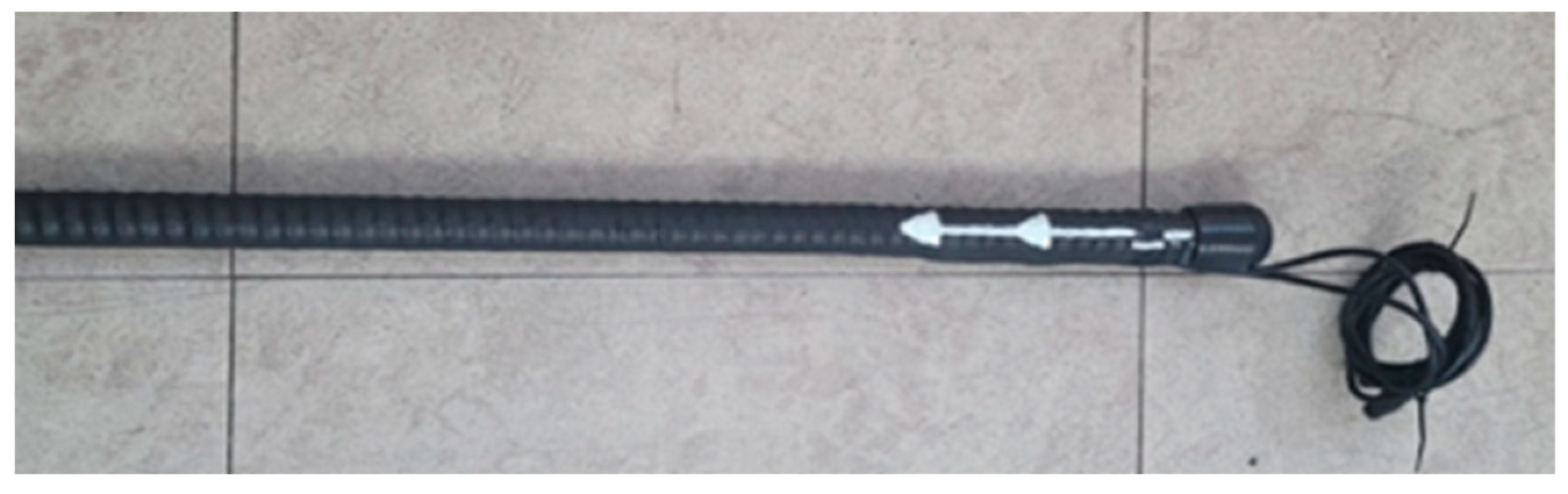
The monitoring site is a steep, weathered-soil slope located adjacent to a residential area in Seocheon, Republic of Korea. To observe slope deformation, a network of GFRP rock-bolt-type sensors was installed along the slope face. GFRP rock bolts (3000 mm in length and 30 mm in diameter) were selected for long-term monitoring because they support practical field deployment, are lightweight, provide strong corrosion resistance, and exhibit less temperature-dependent variability in mechanical properties than conventional metallic reinforcement (Figure 1). Each GFRP rock-bolt sensor was embedded and grouted in a borehole so that ground movement was transferred to the rod, where internal strain gauge measurements were converted to displacement (and derived velocity) via the data logger calibration. In field operation, the system typically exhibits long quasi-static periods with intermittent step-like changes once deformation exceeds the effective sensing/logging resolution; accordingly, we analyzed both displacement and velocity as kinematic indicators for early warning. This configuration is particularly suitable for site-scale monitoring of slopes near critical assets (e.g., residential areas and transportation corridors), where continuous, high-frequency in situ measurements are needed to complement remote sensing and enable timely intervention.

These attributes have been reported as advantageous for reinforced slope monitoring using instrumented GFRP rock-bolt sensors [39]. In addition, recent studies on ground-reinforcement systems emphasize that integrating sensing functions into reinforcement elements enables continuous condition tracking and facilitates proactive intervention. At the same time, the literature notes key practical issues, including calibration sensitivity, potential sensor malfunction, and challenges in interpreting sensor responses, all of which must be addressed in field deployment [40].

Each GFRP rod was equipped with two strain gauge circuits to measure both axial and lateral deformation components. Specifically, two strain gauges (each with an approximately 5 × 1.9 mm sensing area and bonded to a 12 mm diameter gauge pad) were attached to each rod in orthogonal orientations. This arrangement supports concurrent measurement of axial tensile strain, which is associated with in-depth extension or settlement, and lateral bending strain, which is related to shear deformation or horizontal movement along the bolt. After installation and grouting, the GFRP rods therefore act as combined reinforcement and sensing members, converting ground movement into measurable strain responses. Previous work has shown that instrumented GFRP rock-bolt sensors can capture deformation under shear loading and provide informative indicators of slope instability [39].

To achieve representative spatial coverage, GFRP sensor rods were embedded at critical positions across the slope. The rods were distributed over the slope height and width, with emphasis on locations near residential structures to detect potential differential movement. Each rod was installed within a pre-drilled borehole and fixed using cement grout to ensure mechanical coupling with the surrounding soil and rock, consistent with standard installation procedures reported for instrumented rock-bolt sensing systems [39]. The strain gauge leads were waterproofed and connected to an on-site data acquisition unit. By recording both axial extension and lateral bending responses, the monitoring system yields time-series displacement proxy measurements that characterize slope deformation in two orthogonal directions. This dual-channel configuration improves the ability to distinguish complex kinematic behaviors, such as settlement-dominated motion versus horizontal creep, compared with single-channel sensing. In this manuscript, PRISM-TAD is therefore evaluated as a single-point instability detection algorithm operating on a two-channel time series from one instrumented rod. The objective is method validation under a controlled field case rather than a full spatial early warning deployment. In multi-rod settings, the same detector can be executed per rod to produce calibrated anomaly evidence at each location, and a separate spatial decision layer such as multi-sensor voting, hierarchical fusion, or geometry-aware aggregation can be introduced to translate distributed anomaly patterns into slope level alerts.

The monitored slope was registered and managed by the local government as a high-risk steep slope site due to its proximity to residential infrastructure and its history of instability. The sensing system employed a single embedded GFRP rock-bolt sensor rod, from which two displacement-related measurement channels were recorded (referred to as Sensor 1 and Sensor 2 in this study) and used as the primary inputs for model development and evaluation. Measurements were acquired at a 5 min interval and processed as described in Section 2.2. Notably, the recorded increments exhibit strong quantization (large probability mass at exactly zero), which we report and analyze explicitly as part of the preprocessing sensitivity study.

2.2. Data Acquisition and Preprocessing

Displacement measurements were collected continuously from the slope monitoring system for five months, with observations logged at 5 min intervals through a centralized data logger, producing a high temporal resolution record of slope deformation. The present analysis focuses on a representative monitoring point that exhibited pronounced movement, using one instrumented rod that provides two sensing channels corresponding to axial and lateral deformation.

To attenuate environmental effects, we performed residual correction using a gradient boosting regressor that models the environment-driven component of the displacement as a function of temperature, humidity, and battery voltage. The regressor was trained on an initial stable interval, defined as the earliest contiguous segment used for model fitting and selected conservatively to reduce the likelihood that genuine deformation precursors are treated as environmental noise. In addition to basic data screening, we required that this interval (i) was well separated from the documented failure time, (ii) exhibited no sustained monotonic drift of displacement over multi-day windows, and (iii) showed near-zero kinematic activity (velocity magnitude concentrated around the sensor’s effective deadband, quantization regime). Residual displacement was then computed as the observed displacement minus the regressor prediction, and residual velocity was recomputed by finite differencing of the residual displacement.

However, under a worst-case scenario where true precursor deformation is already present in the stable interval and partially correlated with environmental variables, residual correction could attenuate low-frequency precursor components. For this reason, we treated residual correction as an optional noise reduction step, providing an explicit robustness comparison with and without residual correction in Supplementary Section S4 (Table S4), which bounds the potential suppression effect and improves transparency of the preprocessing assumptions.

To ensure temporal consistency, the raw readings, which contained minor irregularities in logging time, were resampled onto a uniform 5 min grid and completed using linear interpolation. This process established a constant sampling interval of $\Delta \mathrm{t}=5\hspace{0.25em}\mathrm{m}\mathrm{i}\mathrm{n}$ for all subsequent analyses. All timestamps were converted to a standardized datetime format and ordered chronologically to enable consistent downstream processing. To remove offsets associated with initial installation and to emphasize deformation evolution, the raw signals were transformed into relative displacement series. The first valid non-zero observation within the monitoring period was selected as the baseline reference (${\mathrm{t}}_0$), and each subsequent measurement $\mathrm{d}\left(\mathrm{t}\right)$ was converted to a relative displacement $\Delta \mathrm{d}\left(\mathrm{t}\right)$ as $\Delta \mathrm{d}\left(\mathrm{t}\right)=\mathrm{d}\left(\mathrm{t}\right)-\mathrm{d}\left({\mathrm{t}}_0\right)$.

Let the original measurements be $\{\left({\mathrm{t}}_{\mathrm{n}},{\mathrm{d}}_{\mathrm{c}}\left({\mathrm{t}}_{\mathrm{n}}\right)\right){\}}_{\mathrm{n}=1}^{\mathrm{N}}$ for channel $\mathrm{c}\in \left\{\mathrm{1,\; 2}\right\}$, where ${\mathrm{t}}_{\mathrm{n}}$ denotes the recorded timestamps. We constructed a uniform time grid:

$${\mathrm{t}}_{\mathrm{k}}={\mathrm{t}}_{\mathrm{s}\mathrm{t}\mathrm{a}\mathrm{r}\mathrm{t}}+\mathrm{k}\Delta \mathrm{t}, \Delta \mathrm{t}=5\hspace{0.25em}\mathrm{m}\mathrm{i}\mathrm{n}, \mathrm{k}=\mathrm{0,1},\dots ,\mathrm{K}.$$

Any minor irregularities in logging times were handled by linear interpolation. For a grid time ${\mathrm{t}}_{\mathrm{k}}$ lying between two recorded times ${\mathrm{t}}_{\mathrm{n}}\le {\mathrm{t}}_{\mathrm{k}}\le {\mathrm{t}}_{\mathrm{n}+1}$,

$${\tilde{\mathrm{d}}}_{\mathrm{c}}\left({\mathrm{t}}_{\mathrm{k}}\right)={\mathrm{d}}_{\mathrm{c}}\left({\mathrm{t}}_{\mathrm{n}}\right)+{\displaystyle \frac{{\mathrm{d}}_{\mathrm{c}}\left({\mathrm{t}}_{\mathrm{n}+1}\right)-{\mathrm{d}}_{\mathrm{c}}\left({\mathrm{t}}_{\mathrm{n}}\right)}{{\mathrm{t}}_{\mathrm{n}+1}-{\mathrm{t}}_{\mathrm{n}}}}\hspace{0.17em}\left({\mathrm{t}}_{\mathrm{k}}-{\mathrm{t}}_{\mathrm{n}}\right).$$

This yields the uniformly sampled sequence ${\tilde{\mathrm{d}}}_{\mathrm{c}}\left({\mathrm{t}}_{\mathrm{k}}\right)$ for subsequent processing. In addition, displacement velocity was computed as a kinematic indicator relevant to impending instability.

To suppress installation offsets and highlight deformation trends, each channel was converted to a relative displacement series using a baseline time ${\mathrm{t}}_0$. Specifically, ${\mathrm{t}}_0$ was defined as the earliest valid (non-spurious) observation:

$${\mathrm{t}}_0=\mathrm{m}\mathrm{i}\mathrm{n}\{{\mathrm{t}}_{\mathrm{k}}\hspace{0.33em}|\hspace{0.33em}{\tilde{\mathrm{d}}}_{\mathrm{c}}\left({\mathrm{t}}_{\mathrm{k}}\right)\hspace{0.25em}\mathrm{is} \mathrm{valid}\}.$$

Relative displacement was then computed as

$$\Delta {\mathrm{d}}_{\mathrm{c}}\left({\mathrm{t}}_{\mathrm{k}}\right)={\tilde{\mathrm{d}}}_{\mathrm{c}}\left({\mathrm{t}}_{\mathrm{k}}\right)-{\tilde{\mathrm{d}}}_{\mathrm{c}}\left({\mathrm{t}}_0\right).$$

Displacement velocity was estimated by a discrete approximation of the first derivative. Using a backward finite difference on the uniform grid,

$${\mathrm{v}}_{\mathrm{c}}\left({\mathrm{t}}_{\mathrm{k}}\right)={\displaystyle \frac{\Delta {\mathrm{d}}_{\mathrm{c}}\left({\mathrm{t}}_{\mathrm{k}}\right)-\Delta {\mathrm{d}}_{\mathrm{c}}\left({\mathrm{t}}_{\mathrm{k}-1}\right)}{\Delta \mathrm{t}}}, \mathrm{k}=1,\dots ,\mathrm{K},$$

where $\Delta \mathrm{t}=5 \mathrm{m}\mathrm{i}\mathrm{n}$. The resulting ${\mathrm{v}}_1\left({\mathrm{t}}_{\mathrm{k}}\right)$ and ${\mathrm{v}}_2\left({\mathrm{t}}_{\mathrm{k}}\right)$ represent the axial and lateral deformation rates, respectively. Explicitly incorporating velocity introduces a kinematic prior that supports detection of acceleration patterns that are often associated with progressive instability.

Environmental measurements, including air temperature $\mathrm{T}\left({\mathrm{t}}_{\mathrm{k}}\right)$, relative humidity $\mathrm{H}\left({\mathrm{t}}_{\mathrm{k}}\right)$, and battery voltage $\mathrm{B}\left({\mathrm{t}}_{\mathrm{k}}\right)$ can induce systematic drift in displacement measurements. To reduce this influence, we trained a gradient boosting regression model ${\mathrm{f}}_{\mathrm{c}}\left(·\right)$ using the initial training segment to estimate the environment-driven displacement component:

$${\widehat{\Delta \mathrm{d}}}_{\mathrm{c}}^{\hspace{0.17em}\mathrm{e}\mathrm{n}\mathrm{v}}\left({\mathrm{t}}_{\mathrm{k}}\right)={\mathrm{f}}_{\mathrm{c}}\left(\mathrm{T}\left({\mathrm{t}}_{\mathrm{k}}\right),\mathrm{H}\left({\mathrm{t}}_{\mathrm{k}}\right),\mathrm{B}\left({\mathrm{t}}_{\mathrm{k}}\right)\right).$$

Residual displacement was obtained by subtracting the predicted environmental contribution:

$$\Delta {\mathrm{d}}_{\mathrm{c}}^{\mathrm{r}\mathrm{e}\mathrm{s}}\left({\mathrm{t}}_{\mathrm{k}}\right)=\Delta {\mathrm{d}}_{\mathrm{c}}\left({\mathrm{t}}_{\mathrm{k}}\right)-{\widehat{\Delta \mathrm{d}}}_{\mathrm{c}}^{\hspace{0.17em}\mathrm{e}\mathrm{n}\mathrm{v}}\left({\mathrm{t}}_{\mathrm{k}}\right).$$

Residual velocities were recomputed in the same manner:

$${\mathrm{v}}_{\mathrm{c}}^{\mathrm{r}\mathrm{e}\mathrm{s}}\left({\mathrm{t}}_{\mathrm{k}}\right)={\displaystyle \frac{\Delta {\mathrm{d}}_{\mathrm{c}}^{\mathrm{r}\mathrm{e}\mathrm{s}}\left({\mathrm{t}}_{\mathrm{k}}\right)-\Delta {\mathrm{d}}_{\mathrm{c}}^{\mathrm{r}\mathrm{e}\mathrm{s}}\left({\mathrm{t}}_{\mathrm{k}-1}\right)}{\Delta \mathrm{t}}}.$$

This correction reduces correlations with environmental fluctuations and thereby emphasizes deformation signals of geotechnical or structural origin for anomaly detection.

Finally, each feature $\mathrm{x}\left({\mathrm{t}}_{\mathrm{k}}\right)$ (e.g., $\Delta {\mathrm{d}}_{\mathrm{c}}^{\mathrm{r}\mathrm{e}\mathrm{s}}\left({\mathrm{t}}_{\mathrm{k}}\right)$, ${\mathrm{v}}_{\mathrm{c}}^{\mathrm{r}\mathrm{e}\mathrm{s}}\left({\mathrm{t}}_{\mathrm{k}}\right)$, or the corresponding non-residual variables) was robustly normalized using training subset statistics. Let

$$\mathrm{m}\mathrm{e}\mathrm{d}\left(\mathrm{x}\right)=\mathrm{m}\mathrm{e}\mathrm{d}\mathrm{i}\mathrm{a}\mathrm{n}\left\{\mathrm{x}\left({\mathrm{t}}_{\mathrm{k}}\right)\right\},\mathrm{M}\mathrm{A}\mathrm{D}\left(\mathrm{x}\right)=\mathrm{m}\mathrm{e}\mathrm{d}\mathrm{i}\mathrm{a}\mathrm{n}\left\{\left|\mathrm{x}\left({\mathrm{t}}_{\mathrm{k}}\right)-\mathrm{m}\mathrm{e}\mathrm{d}\left(\mathrm{x}\right)\right|\right\}.$$

The scaled feature is

$${\mathrm{x}}^{\mathrm{s}\mathrm{c}}\left({\mathrm{t}}_{\mathrm{k}}\right)={\displaystyle \frac{\mathrm{x}\left({\mathrm{t}}_{\mathrm{k}}\right)-\mathrm{m}\mathrm{e}\mathrm{d}\left(\mathrm{x}\right)}{\mathrm{M}\mathrm{A}\mathrm{D}\left(\mathrm{x}\right)+\mathsf{\epsilon }}},$$

where a small $\mathsf{\epsilon }>0$ avoids division by zero. This robust scaling reduces sensitivity to extreme outliers while preserving the relative structure of anomalous behavior [41].

2.3. Anomaly Detection Models

To identify early warning signatures of slope instability, we implemented and compared a heterogeneous set of anomaly detection methods spanning threshold-based screening, classical machine learning outlier detectors, and deep learning models. This selection includes commonly used practical baselines as well as advanced algorithms, providing a comprehensive benchmark for evaluating the proposed approach. All models were implemented and trained in Python 3.12. The compared methods are summarized below.

The first model is Robust Z-Score Velocity (RobustZVel). This threshold-based baseline applies robust statistics to the velocity features to flag atypical increases in movement rate. During training, the method computes the median and median absolute deviation (MAD) of the velocity magnitude. At time $\mathrm{t}$, the anomaly score is defined as the maximum robust z-score across velocity channels:

$$\mathrm{s}\left(\mathrm{t}\right)=\underset{\mathrm{i}}{\max }\left|{\displaystyle \frac{{\mathrm{v}}_{\mathrm{i}}\left(\mathrm{t}\right)-\mathrm{m}\mathrm{d}\mathrm{e}\mathrm{i}\mathrm{a}\mathrm{n}\left({\mathrm{v}}_{\mathrm{i}}\right)}{\mathrm{M}\mathrm{A}\mathrm{D}\left({\mathrm{v}}_{\mathrm{i}}\right)}}\right|.$$

This formulation highlights time points at which the displacement rate is unusually high relative to typical variability. Such rule-based criteria resemble operational warning logic in many early warning settings, where alerts are issued when deformation rates exceed predefined limits. The use of the median and MAD improves robustness to outliers and is intended to emphasize persistent velocity increases rather than transient noise.

The second model is Principal Component Analysis Reconstruction (PCA-Recon). PCA is a linear dimensionality reduction technique, used here to capture the normal correlation structure of the multivariate sequence. A sliding window of length $\mathrm{W}$ is moved across the time series, and each window is flattened into a feature vector. A PCA model is fitted to training window vectors, retaining sufficient components to explain 95% of the variance. For an unseen window, the PCA reconstruction is computed and the reconstruction error (mean squared error between the original vector and its reconstruction) is used as the anomaly score. The underlying rationale is that windows containing atypical patterns, such as abrupt jumps or shifts not represented in training, are poorly captured by the principal subspace and therefore produce elevated reconstruction errors. In this study, PCA-Recon serves as a baseline for modeling linear relationships between the two deformation channels and their temporal evolution. The third model is Isolation Forest. Isolation Forest is an ensemble anomaly detection method that isolates observations using randomly constructed decision trees, exploiting the principle that anomalies are rare and distinct and therefore tend to be separated with fewer splits. We applied Isolation Forest to the same sliding window vectors of the multivariate series. The method randomly selects features and split thresholds to partition the data, and windows that require fewer splits on average to isolate receive higher anomaly scores. We used an ensemble of 300 trees with automatic contamination setting. The anomaly score is derived from the negative average path length in the forest, where shorter paths correspond to greater anomalousness. Isolation Forest imposes minimal distributional assumptions and is widely used for efficient unsupervised outlier detection.

The fourth model is One-Class SVM (OC-SVM). The one-class support vector machine is a kernel-based novelty detector that learns the boundary of normal data in feature space and labels points outside this boundary as anomalous. We trained an OC-SVM using the windowed feature vectors with a radial basis function (RBF) kernel. The $\mathsf{\nu }$ parameter, controlling the fraction of support vectors and the tightness of the boundary, was set to 0.02 to yield a compact envelope around the training data. OC-SVM provides a classical baseline for capturing nonlinear relationships between axial and lateral deformation features. Unseen combinations of trends or abrupt changes that deviate from the learned normal manifold result in large anomaly scores, computed as the negative distance to the decision boundary.

The fifth baseline model is a 1D Convolutional Autoencoder (Conv1D-AE). As a representative deep learning benchmark, we developed a convolutional autoencoder to learn normal time-series patterns in an unsupervised manner. The network comprises an encoder that applies stacked 1D convolution layers to compress a multivariate window into a low-dimensional latent representation, and a decoder that reconstructs the input from the latent code. In our implementation, the encoder includes two 1D convolution layers (64 filters followed by 32 latent filters, kernel size 5) with ReLU activations, and the decoder mirrors this structure to reconstruct the original two-channel sequence. The model is trained on sliding windows from the training set by minimizing reconstruction error using mean squared error loss. During inference, the reconstruction error for each window is used as the anomaly score, under the assumption that windows containing deviations from normal behavior are reconstructed poorly. Training was performed for 100 epochs using the Adam optimizer (learning rate ${10}^{-3}$) with a mini-batch size of 128. Autoencoder-based reconstruction has been widely used in monitoring contexts because it can capture complex temporal patterns and flag deviations without requiring explicit anomaly labels.

The sixth baseline is a Transformer Reconstruction Model. To leverage the ability of attention mechanisms to capture long-range temporal structure, we also evaluated an encoder-only Transformer reconstructor. Each multivariate window is first mapped via a linear projection to an embedding of dimension d = 64, processed by a Transformer encoder with two layers and four attention heads (dropout 0.1), and then projected back to the original feature dimension for reconstruction. Similar to Conv1D-AE, the model is trained to minimize reconstruction error on training windows. The anomaly score is defined as the reconstruction mean squared error for each window. Training was conducted for 100 epochs using the same optimization settings as Conv1D-AE. By comparing the Transformer reconstructor with the convolutional autoencoder, we assessed the value of attention-based modeling for slope deformation sequences.

All models listed in items operate on sliding windows of the time series. We evaluated multiple window lengths W to examine sensitivity to temporal scale. Windows were advanced with a stride of one step (5 min), producing a continuous anomaly score time line for each method. Hyperparameters such as the number of retained PCA components, the number of trees in Isolation Forest, the SVM kernel settings, and network architecture choices were kept as defaults or selected through preliminary trials to ensure that each baseline was represented under reasonable and stable configurations.

2.4. Proposed Method: PRISM-TAD

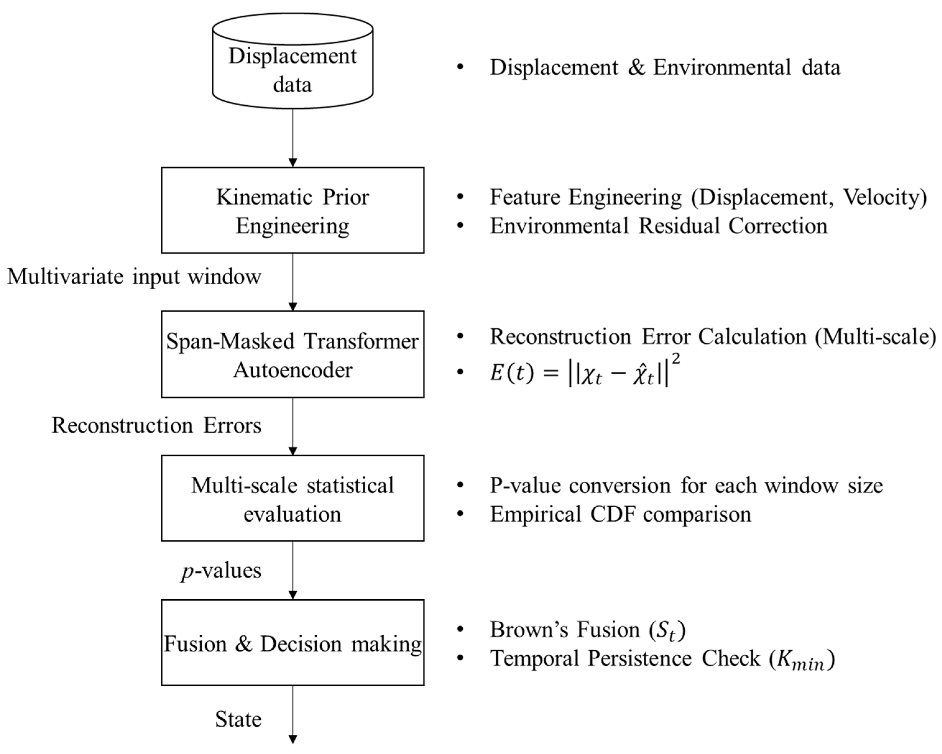
PRISM-TAD is an anomaly detection framework designed for slope failure early warning that integrates slope kinematics domain knowledge with data-driven sequence modeling. The acronym PRISM-TAD denotes Prior Residual Integration and Span-Masked Transformer for Anomaly Detection. The overall workflow comprises the components summarized in Figure 2.

PRISM-TAD uses an augmented input representation that includes displacement and velocity for each sensing channel, together with environmentally residualized signals when available, as described in Section 2.2. By providing displacement–velocity pairs to the model, we embed a physically motivated prior: the displacement derivative is informative for identifying accelerating motion. This design is motivated by the observation that acceleration in deformation frequently precedes collapse, and explicitly incorporating velocity can therefore improve sensitivity to incipient instability. The use of residualized variables further encourages the model to concentrate on mechanically driven deformation rather than environmentally induced drift.

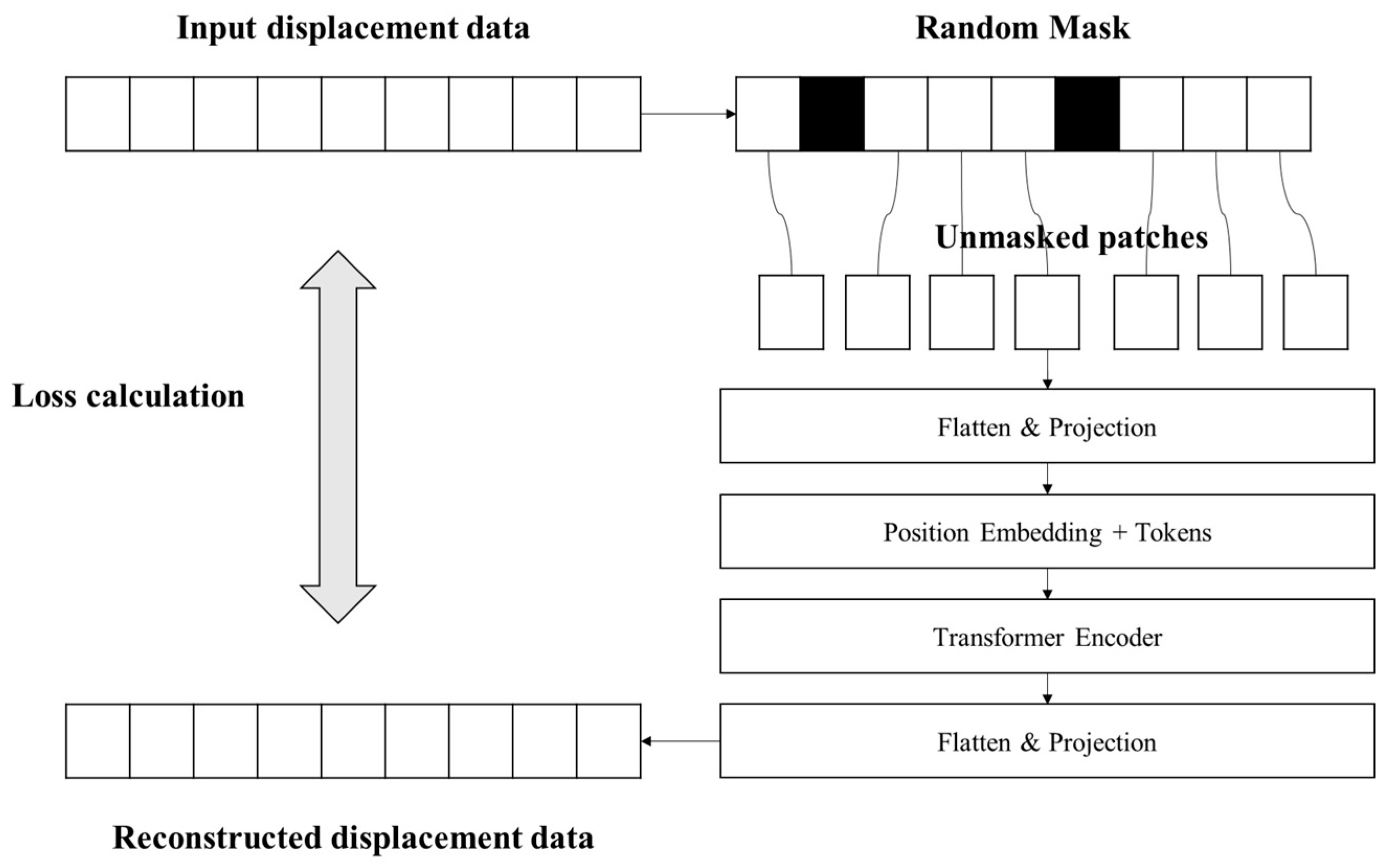
The core of PRISM-TAD is a Transformer-based sequence model trained under a span-masking reconstruction objective. The network follows an encoder-only Transformer configuration consistent with Section 2.3 (two encoder layers, four attention heads, and 64-dimensional embeddings), while the training strategy is modified to enhance robustness. Rather than reconstructing the full input sequence in every iteration, the model is trained to recover randomly masked contiguous segments of the time series. During each training batch, approximately 25% of time steps within each window are masked by replacing them with a learned mask token, with span lengths sampled randomly between 2 and 10 steps (Figure 3). During training, we applied contiguous span masking and optimized reconstruction loss only on masked positions to discourage trivial point-wise interpolation and to encourage learning of non-local temporal structure. The masking ratio controls the degree of contextual inference required: very small ratios can permit reconstruction dominated by short-range interpolation in strongly autocorrelated segments, whereas very large ratios can make reconstruction ill-posed and degrade representation learning stability. Based on these considerations, we set the span-masking ratio to 25% as a moderate corruption level.

To strengthen the robustness of this empirical choice under temporally continuous landslide monitoring data, we performed a sensitivity analysis by varying the masking ratio among {0.10, 0.25, 0.40} while keeping all other settings (data split, calibration protocol, threshold quantile, and persistence rule) unchanged. The fused anomaly score trajectories were highly consistent across ratios (Pearson r = 0.91–0.95) and the resulting false alarm burden remained comparable (0.448–0.580 alarms/day), with 25% providing the lowest false alarm rate among the tested values. Detailed results, including the score evolution, are provided in Supplementary Section S3. With a 5 min sampling interval and window lengths of 1–16 h, this corresponds to reconstructing missing spans on the order of 15 min to 4 h, which is practically relevant for field monitoring gaps. We therefore adopted 25% to promote robustness without over-tuning hyperparameters in a single-event case study.

This objective forces the model to infer missing values from the surrounding temporal context, thereby functioning as both data augmentation and regularization. The model cannot rely on direct memorization of the training sequences; instead, it must learn a representation of normal slope behavior that supports accurate imputation. Conceptually, this corresponds to masked modeling in natural language processing adapted to time-series signals. We implemented the approach in PyTorch 2.8, resampling mask locations for each window at each epoch. The model was trained for 100 epochs using the Adam optimizer with a loss defined only over masked positions, which concentrates learning on predictive reconstruction of missing segments. After training, the encoder can reliably reconstruct normal patterns even under partial observability, while anomalous patterns tend to yield larger reconstruction errors.

At inference time, the model processes each incoming window without masking. Let ${\mathrm{x}}_{\mathrm{t}-\mathrm{W}+1:\mathrm{t}}\in {\mathbb{R}}^{\mathrm{W}\times \mathrm{d}}$ denote the multivariate input window of length $\mathrm{W}$ ending at time $\mathrm{t}$, and let ${\widehat{\mathrm{x}}}_{\mathrm{t}-\mathrm{W}+1:\mathrm{t}}$ be its reconstruction. We define the mean squared reconstruction error as

$$\mathrm{e}\left(\mathrm{t};\mathrm{W}\right)={\displaystyle \frac{1}{\mathrm{W}\mathrm{d}}}\sum _{\mathrm{i}=0}^{\mathrm{W}-1}{∥{\mathrm{x}}_{\mathrm{t}-\mathrm{i}}-{\widehat{\mathrm{x}}}_{\mathrm{t}-\mathrm{i}}∥}_2^2$$

A larger value of $\mathrm{e}(\mathrm{t};\mathrm{W})$ indicates that the observed window is difficult to reproduce under the learned normal pattern model and is therefore more likely to be anomalous. To obtain a statistically interpretable anomaly measure, we mapped $\mathrm{e}(\mathrm{t};\mathrm{W})$ to an empirical p-value by comparing it with the reconstruction error distribution computed on training windows:

$${\mathrm{p}}_{\mathrm{W}}\left(\mathrm{t}\right)=\mathrm{P}\mathrm{r}\left({\mathrm{e}}^{\mathrm{t}\mathrm{r}\mathrm{a}\mathrm{i}\mathrm{n}}\left(\mathrm{W}\right)\ge \mathrm{e}\left(\mathrm{t};\mathrm{W}\right)\right)={\displaystyle \frac{1}{{\mathrm{N}}_{\mathrm{W}}}}\sum _{\mathrm{n}=1}^{{\mathrm{N}}_{\mathrm{W}}}1\left[{\mathrm{e}}_{\mathrm{n}}^{\mathrm{t}\mathrm{r}\mathrm{a}\mathrm{i}\mathrm{n}}\left(\mathrm{W}\right)\ge \mathrm{e}\left(\mathrm{t};\mathrm{W}\right)\right],$$

where $1\left[·\right]$ is the indicator function. When $\mathrm{K}$ different window lengths $\{{\mathrm{W}}_{\mathrm{j}}{\}}_{\mathrm{j}=1}^{\mathrm{K}}$ are used, these p-values form an anomaly p-value vector $\mathrm{P}\left(\mathrm{t}\right)=\left[{\mathrm{p}}_{{\mathrm{W}}_1}\left(\mathrm{t}\right),\hspace{0.17em}{\mathrm{p}}_{{\mathrm{W}}_2}\left(\mathrm{t}\right),\hspace{0.17em}\dots ,\hspace{0.17em}{\mathrm{p}}_{{\mathrm{W}}_{\mathrm{K}}}\left(\mathrm{t}\right)\right]$.

A small p-value indicates that the current window error lies in the extreme tail of the normal error distribution, implying a statistically unlikely pattern under nominal conditions.

Indicators of instability may arise at different temporal scales. Abrupt deviations are often detectable using short windows, whereas gradual changes may be more evident at longer horizons. To exploit this multi-scale structure, PRISM-TAD aggregates evidence across multiple window lengths using Brown’s method, which adjusts Fisher type p-value combination to account for dependence among tests induced by overlapping and nested sliding windows. Let ${\mathrm{p}}_{\mathrm{j}}(\mathrm{t})$ denote the window-level p-value at time $\mathrm{t}$ for the $\mathrm{j}$-th window length $(\mathrm{j}=\mathrm{1,2},\dots ,\mathrm{K})$. We first computed the Fisher type statistic:

$$\mathrm{S}\left(\mathrm{t}\right)=-2\sum _{\mathrm{j}=1}^{\mathrm{K}}\mathrm{l}\mathrm{n}\left({\mathrm{p}}_{\mathrm{j}}\left(\mathrm{t}\right)\right),$$

Because $\{{\mathrm{p}}_{\mathrm{j}}(\mathrm{t})\}$ are correlated across window lengths, Brown’s method approximates the null distribution of $\mathrm{S}\left(\mathrm{t}\right)$ as a scaled chi-square:

$$\mathrm{S}\left(\mathrm{t}\right)\sim {\mathrm{c}\mathsf{\chi }}_{\mathsf{\nu }}^2$$

where the scale ccc and degrees of freedom $\mathsf{\nu }$ are determined by matching the first two moments of $\mathrm{S}\left(\mathrm{t}\right)$ under nominal conditions. Specifically, define ${\mathrm{X}}_{\mathrm{j}}(\mathrm{t})=-2\ln {\mathrm{p}}_{\mathrm{j}}(\mathrm{t})$, so that $\mathrm{S}(\mathrm{t})={\sum }_{\mathrm{j}}{\mathrm{X}}_{\mathrm{j}}(\mathrm{t})$. Under the null, $\mathsf{\mu }=\mathrm{E}\left[\mathrm{S}\right]=2\mathrm{K}$, while ${\mathsf{\sigma }}^2=\mathrm{V}\mathrm{a}\mathrm{r}(\mathrm{S})$ is estimated from a held-out normal calibration set via the empirical covariance of $\left\{{\mathrm{X}}_{\mathrm{j}}\left(\mathrm{t}\right)\right\}$. The Brown parameters are then set as

$$\mathrm{c}={\mathsf{\sigma }}^2/2\mathsf{\mu }, \mathsf{\nu }=2{\mathsf{\mu }}^2/{\mathsf{\sigma }}^2$$

Equivalently, a dependence-adjusted fused p-value can be obtained as

$${\mathrm{p}}_{\mathrm{f}\mathrm{u}\mathrm{s}\mathrm{i}\mathrm{o}\mathrm{n}}\left(\mathrm{t}\right)=1-{\mathrm{F}}_{{\mathsf{\chi }}_{\mathsf{\nu }}^2}\left({\displaystyle \frac{\mathrm{S}\left(\mathrm{t}\right)}{\mathrm{c}}}\right),$$

where ${\mathrm{F}}_{{\mathsf{\chi }}_{\mathsf{\nu }}^2}\left(·\right)$ is the CDF of ${\mathsf{\chi }}_{\mathsf{\nu }}^2$. In this study, we used $\mathrm{K}=5$ window lengths corresponding to 1 h, 2 h, 4 h, 8 h, and 16 h. To control false alarms in operation, the fused score (we used ${\mathrm{T}}_{\mathrm{f}\mathrm{u}\mathrm{s}\mathrm{i}\mathrm{o}\mathrm{n}}\left(\mathrm{t}\right)=\mathrm{S}\left(\mathrm{t}\right)$; equivalently, any monotone transform of ${\mathrm{p}}_{\mathrm{f}\mathrm{u}\mathrm{s}\mathrm{i}\mathrm{o}\mathrm{n}}(\mathrm{t}))$ is calibrated using a held-out normal calibration set. Let $\{{\mathrm{T}}_{\mathrm{f}\mathrm{u}\mathrm{s}\mathrm{i}\mathrm{o}\mathrm{n}}^{\mathrm{c}\mathrm{a}\mathrm{l}}\left(\mathrm{t}\right)\}$ denote fused scores on the calibration data. For a target false alarm quantile $\mathrm{q}$ (e.g., $\mathrm{q}=0.95$), we set the detection threshold as

$${\mathrm{T}}^{\star }={\mathrm{Q}}_{\mathrm{q}}\left(\left\{{\mathrm{T}}_{\mathrm{f}\mathrm{u}\mathrm{s}\mathrm{i}\mathrm{o}\mathrm{n}}^{\mathrm{c}\mathrm{a}\mathrm{l}}\left(\mathrm{t}\right)\right\}\right),$$

where ${\mathrm{Q}}_{\mathrm{q}}\left(·\right)$ is the empirical $\mathrm{q}$-quantile. An observation at time $\mathrm{t}$ is labeled anomalous when ${\mathrm{T}}_{\mathrm{f}\mathrm{u}\mathrm{s}\mathrm{i}\mathrm{o}\mathrm{n}}\left(\mathrm{t}\right)>{\mathrm{T}}^{\mathrm{*}}$. This fusion-and-calibration procedure consolidates multi-scale evidence and improves robustness by reducing sensitivity to any single window length.

To further suppress transient artifacts and spurious alarms, PRISM-TAD applies a persistence requirement. A warning is issued only when the anomaly condition holds for at least $\mathrm{k}$ consecutive time steps. In our implementation, $\mathrm{k}=3$, corresponding to 15 min of persistence under a 5 min sampling interval. The alarm rule is

$$\mathrm{A}\mathrm{l}\mathrm{a}\mathrm{r}\mathrm{m}\left(\mathrm{t}\right)=1\left[\sum _{\mathrm{i}=0}^{\mathrm{k}-1}\mathrm{a}\left(\mathrm{t}-\mathrm{i}\right)=\mathrm{k}\right].$$

This persistence check ensures that alerts correspond to sustained departures from nominal behavior, consistent with operational early warning practices that seek to reduce false alarms triggered by momentary noise.

2.5. Evaluation Procedure

The anomaly detection methods were assessed using both continuous score metrics and event-oriented early warning criteria under a chronological train calibration test split. The monitoring dataset contains 51,951 observations per channel sampled at 5 min intervals, with no missing values. The record spans from the start of sensor operation to the documented slope failure event on 17 July 2025 (KST), as summarized in

Table 1. Summary statistics of collected displacement data.

Statistical Metrics	Sensor 1	Sensor 2
Samples	51,951	51,951
Missing rate (%)	0	0
Zero rate (%)	99.13	84.93
Mean (mm)	0.0274	0.140277

. Zero-value prevalence and handling. Table 1 reports a high fraction of samples recorded as exactly zero. Here, a “zero” is defined as a raw displacement value that equals 0.0 after conversion from the data logger output to engineering units. It is not a missing entry (the missing rate is 0%). Such zero-valued segments can arise in long-term embedded monitoring due to finite sensor resolution and quantization near small strains, deadband behavior around near-static states, and/or intermittent acquisition/communication behaviors that return a default or repeated value.

To make this characteristic explicit, we report two additional diagnostics: (i) the distribution of zero-run lengths (consecutive samples equal to zero) and (ii) the empirical distribution of non-zero increments and their timing. These summaries quantify the effective temporal granularity at which the instrument expresses deformation and helps distinguish “no motion” from “motion below resolution.”

From a modeling perspective, strong zero inflation can affect anomaly detection in two opposite ways. First, reconstruction-based detectors may achieve artificially low errors on plateau segments because constant signals are easy to reproduce, which can reduce sensitivity if the onset of instability is expressed as gradual sub-resolution creep. Second, when deformation exceeds the deadband, the resulting step changes induce abrupt local nonstationarity that can elevate reconstruction errors and thus improve detectability. Our pipeline partially mitigates plateau dominance by incorporating derived velocity features (finite differences), which transform step changes into sparse but salient impulses, and by calibrating alarm thresholds on a held-out nominal calibration subset using a consistent exceedance quantile.

To verify that the unusually high zero-value rate does not artificially drive detection behavior, we performed a zero-inflation robustness check using activity-augmented and de-quantized (jittered) representations in Supplementary Section S2 and Table S2.

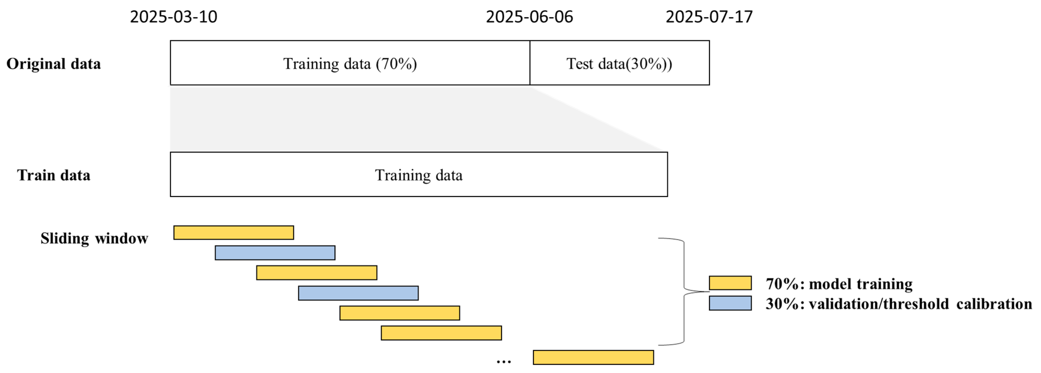
The full timeline was divided into a development segment (first 70%) and a held-out test segment (final 30%), with the test segment ending at the known failure time to emulate prospective deployment (Figure 4). Within the development segment, we further separated a fitting subset (first 70% of development) and a calibration subset (remaining 30% of development). Model fitting (including normalization statistics) used only the fitting subset to avoid look-ahead bias. The calibration subset was used exclusively to select alert thresholds.

Each detector produced an anomaly score sequence on the calibration subset. To harmonize operational sensitivity across methods, an algorithm-specific alarm threshold was defined as the 95th percentile of the calibration scores, corresponding to an exceedance probability of 5% on calibration data. This rule provides a consistent and interpretable calibration protocol across detectors, while recognizing that the realized false alarm frequency in the test period may differ due to score autocorrelation and differences in score distributions. While the 95th-percentile calibration aligns detectors at a comparable nominal exceedance rate on the calibration subset, the realized false alarm frequency in the test period can differ across methods due to score autocorrelation, tail heaviness, and differing score smoothness. For this reason, we report both threshold-dependent operational metrics (false alarms/day, lead time) and threshold-swept metrics to provide a more complete and fair comparison. The same thresholding procedure was applied to the fused PRISM-TAD statistic. To reduce short-lived fluctuations, a temporal persistence criterion was imposed for all methods: an alert was issued only when the anomaly condition was satisfied for at least three consecutive 5 min samples, equivalent to 15 min.

Because dense ground-truth labels are not available in field monitoring, we constructed proxy labels relative to the known failure time $t_{fail}$. For a selected warning horizon $\mathrm{H} (\mathrm{e}.\mathrm{g}., \mathrm{H}=24 \mathrm{h})$, samples with $[{\mathrm{t}}_{\mathrm{f}\mathrm{a}\mathrm{i}\mathrm{l}}-H, t_{fail}]$ were treated as positives representing the pre-failure interval, whereas samples prior to ${\mathrm{t}}_{\mathrm{f}\mathrm{a}\mathrm{i}\mathrm{l}}-H$ were treated as negatives. Using thresholded and persisted alarms, we computed precision, recall, and F1-score, together with the false alarm rate, expressed as alarms per day within the negative interval. In addition, we quantified threshold-independent discriminative performance using ROC AUC and precision recall curves obtained by sweeping the anomaly threshold. These metrics evaluate how effectively each model separates pre-failure behavior from the extended nominal period under strong class imbalance.

Beyond pointwise classification, we evaluated operational early warning performance with respect to the failure event. A run was considered successful if at least one persisted alarm occurred within the final $\mathrm{H}$ hours preceding ${\mathrm{t}}_{\mathrm{f}\mathrm{a}\mathrm{i}\mathrm{l}}$. For successful runs, we report the lead time of the first alarm ${\mathrm{t}}_{\mathrm{f}\mathrm{a}\mathrm{i}\mathrm{l}}-t_{alarm}$ and) and the false alarm frequency over the negative interval. This event-level perspective reflects practical requirements: warnings must provide actionable lead time while remaining sufficiently infrequent to prevent alarm fatigue.

3. Results

This section reports the performance of the proposed PRISM-TAD framework relative to baseline detectors for slope failure early warning. The results indicate that PRISM-TAD provides timely warnings with substantially fewer false alarms while preserving high detection precision and stable behavior across the evaluated settings.

3.1. Early Warning Performance

Operational early warning systems for slope failure must provide sufficient lead time for response while keeping the false alarm burden within a manageable range. Here, warnings are evaluated using a pre-failure horizon of $\mathrm{H}=24 \mathrm{h}$ as a standardized assessment window referenced to the documented collapse time. This horizon is not intended to imply that precursory signals always emerge exactly 24 h prior to failure; rather, it defines a consistent and practically relevant last-day warning objective for comparing detectors.

Table 2. Detection performance of PRISM-TAD and baselines at a common operating point. “Detection” indicates at least one alarm within the last $\mathrm{H}$ hours before failure ($\mathrm{H}=24 \mathrm{h}$). “Median detection delay” is measured from ${\mathrm{t}}_{\mathrm{f}\mathrm{a}\mathrm{i}\mathrm{l}}-\mathrm{H}$ to the first alarm. “False alarms/day” is the average number of alarms per day for $\mathrm{t}<{\mathrm{t}}_{\mathrm{t}\mathrm{a}\mathrm{i}\mathrm{l}}-\mathrm{H}$. Thresholds are calibrated at the 95th percentile; persistence $\mathrm{k}=3$ (15 min).

Model	Detection	Median Detection Delay	False Alarms per Day
PRISM-TAD (Proposed)	Yes	105 min	0.45
RobustZVel	No	– (no alarm)	0 (no alarm)
PCARecon	Yes	0	1.06
Isolation Forest	Yes	0	0.71
OneClass SVM	Yes	0	0.65
Conv1D Autoencoder	Yes	0	0.69
Transformer Recon	Yes	0	1.08

summarizes event-level warning outcomes at the calibrated operating point. PRISM-TAD generated a sustained alarm within the 24 h window and exhibited a median detection delay of 105 min measured from the beginning of the 24 h interval. This corresponds to an initial warning approximately 22 h 15 min before the recorded failure time, accounting for the 15 min persistence requirement. Several baseline methods can be configured to trigger near the start of the 24 h window if thresholds are set aggressively; however, such high-sensitivity configurations typically produce frequent false alerts during nominal conditions. From an operational perspective, the central question is therefore not whether an algorithm can be forced to alarm as early as possible, but whether it can provide early alarms while maintaining an acceptable false alarm frequency.

When baseline methods are constrained to lower false alarm rates, warning timeliness often deteriorates markedly, and in some cases, the pre-failure alert is not produced. For example, OneClassSVM can be adjusted to reduce spurious alerts, but the first detection may then occur after the pre-failure horizon, which is operationally ineffective. In contrast, PRISM-TAD retains early warning capability while maintaining comparatively low false alarm frequency under the same calibration protocol. Overall, these results suggest that PRISM-TAD achieves a more favorable operational trade-off by providing multi-hour lead time within the last-day window without relying on excessively sensitive threshold settings that would be unsuitable for continuous monitoring.

3.2. False Alarm Rate and Detection Precision

In operational settings, limiting false alarms is as important as achieving early detection because frequent false alerts can induce alarm fatigue and impose substantial response costs. As shown in Table 2, PRISM-TAD substantially reduced false alarm frequency compared with the baseline methods. Across the long-term monitoring period, PRISM-TAD produced an average of 0.45 spurious alarm onsets per day. This rate is approximately half that of the best-performing baseline at comparable sensitivity and several times lower than more aggressive baseline configurations. For instance, PCARecon and TransformerRecon generated more than one false alarm per day on average, whereas PRISM-TAD remained below 0.5 per day. Isolation Forest and the Conv1D Autoencoder exhibited intermediate false alarm frequencies of roughly 0.7 per day, which is still approximately 40% to 50% higher than PRISM-TAD. Although methods such as OneClassSVM can be tuned to reduce false alarms, doing so typically results in delayed detection or missed warnings. PRISM-TAD therefore provides a strong combination of reduced false positives while preserving event detection capability.

The improved alarm precision of PRISM-TAD is consistent with its enhanced ability to separate true precursory behavior from normal fluctuations. Quantitatively, PRISM-TAD achieved the highest ROC AUC among the compared methods, indicating the most favorable overall balance between true positive and false positive rates.

All remaining baselines showed lower discriminative performance, with AUC values ranging from 0.58 to 0.84. RobustZVel performed worst, with an AUC of 0.58. The higher AUC for PRISM-TAD indicates that it more consistently assigns higher anomaly scores to genuine instability-related signals than to routine variability, thereby reducing both missed detections and false alarms. In practical terms, during extended monitoring periods in which failure events are rare, baseline methods tended to generate numerous false alarm episodes relative to true events, whereas PRISM-TAD produced fewer alarm occurrences and consequently achieved a higher fraction of meaningful alerts.

Beyond the calibrated operating point results in Table 2, we also assessed threshold-swept discrimination using pre-failure proxy labels. Positive samples were defined within the last H hours before the recorded failure time, and negatives were defined as those occurring earlier. Because the present dataset contains a single failure event and exhibits extreme class imbalance, such threshold-swept metrics (ROC-AUC and PR-AUC) can be sensitive to the exact labeling horizon and evaluation range; therefore, we report them in Supplementary Section S4 (Table S4), together with the corresponding robustness comparison with and without environmental residual correction.

4. Discussion

The evaluation indicates that effective long-term slope monitoring depends not only on detection sensitivity but also on operational stability under non-ideal conditions, such as measurement noise, environmental drift, and time-varying slope behavior. Many baseline detectors are highly sensitive to user-specified settings, including window length and alarm thresholds, which produce a challenging trade-off between timely detection and frequent non-failure alerts. This parameter sensitivity complicates real-world deployment because configurations that appear effective during a short tuning period may become suboptimal as environmental forcing and geotechnical conditions change over time.

PRISM-TAD reduces this operational instability through two coupled design choices: multi-scale evidence integration and alarm confirmation. First, by evaluating anomalies across multiple window lengths and fusing the resulting evidence, the method can capture both abrupt deviations and slowly evolving trends without requiring selection of a single dominant time scale. Second, the persistence criterion requiring three consecutive exceedances acts as a lightweight confirmation step that filters transient outliers. Combined, these mechanisms reduce the probability that alarms are driven by isolated spikes that are not supported across scales or across adjacent time steps, thereby improving practical reliability.

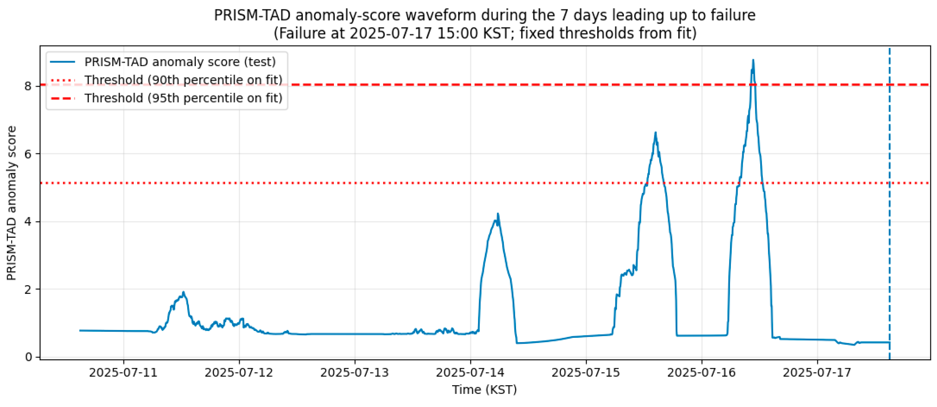
Although PRISM-TAD is formulated as an unsupervised anomaly detector rather than a mechanistic slope stability model, its score is directly driven by deviations in the joint evolution of displacement and velocity from a learned nominal regime. In classical deformation descriptions of progressive instability, monitored slopes may exhibit long quasi-static periods followed by phases of accelerating deformation prior to failure. In our case study, the waveform in Figure 5 shows intermittent score elevations several days before collapse and more sustained exceedances closer to failure. This pattern is consistent with a transition from routine background variability to an acceleration-dominated regime in which the observed kinematics become increasingly difficult to reconstruct using the normal pattern model.

Practically, PRISM-TAD should be interpreted as detecting the onset and persistence of kinematic inconsistency, statistical abnormality, rather than estimating physical parameters such as factor of safety. However, the model’s reliance on velocity-informed inputs makes it naturally sensitive to acceleration-like behavior that is often considered a precursor to instability. Future multi-site validation will examine how consistently specific score regimes correspond to recognized physical processes such as accelerating creep, progressive shear-zone development, or rainfall-driven softening, across varying slope materials and hydrologic conditions. In addition, because the present study evaluates one rod (two channels) and one failure case, extension to spatially distributed monitoring should be understood as requiring an explicit sensor-fusion decision layer in addition to per-sensor detection.

5. Conclusions

This study presents PRISM-TAD, a Transformer-based anomaly detection framework for early warning of slope failure using only historical normal data. In contrast to conventional thresholding approaches and reconstruction-based baselines, PRISM-TAD incorporates a domain-informed kinematic prior and a multi-scale fusion mechanism, enabling detection of subtle and progressive precursors while reducing false alarms.

Evaluation using real slope failure monitoring data demonstrated that PRISM-TAD outperformed six commonly used unsupervised baseline models. PRISM-TAD issued an early warning approximately 22 h prior to the collapse event, achieving lead time comparable to the most responsive baselines while producing substantially fewer false alarms. Although deep learning baselines such as Conv1D-AE and TransformerRecon achieved high recall, they exhibited persistent false positives that limit practical applicability. In contrast, PRISM-TAD delivered actionable lead time within the final day warning horizon while maintaining a low rate of non-failure alarms.

The findings further suggest that PRISM-TAD’s performance is attributable to three design elements: (1) robust identification of spatiotemporal anomalies through multi-scale score fusion, (2) sensitivity to kinematic precursors without excessive amplification of noise, and (3) an empirically calibrated thresholding strategy aligned with operational reliability requirements.

Overall, the results demonstrate that unsupervised anomaly detection, when appropriately regularized and adapted to domain physics, can provide timely and reliable warnings for catastrophic slope failures. Given its strong performance and operational characteristics, PRISM-TAD is a promising candidate for real-world slope failure monitoring systems. Future work will examine generalization across multiple sites and will integrate the framework with real-time data pipelines for continuous operation.