A QGIS-Based Gaussian Plume Dispersion Model for Point Sources: Development and Intercomparison of Reflective and Non-Reflective Formulations

Featured Application

The proposed QGIS-based model is designed as an open-source tool for education, research, and preliminary air quality assessment, enabling rapid estimation and visualization of pollutant dispersion from industrial exhaust stacks. Implemented through an intuitive graphical interface, the model can be used by non-specialists without advanced expertise in programming, dispersion modeling, or Geographical Information System (GIS). This accessibility supports its application in teaching activities, exploratory scenario analysis, and screening-level evaluations of air pollution in urban environments.

Abstract

Air pollution from industrial point sources remains a major concern in urban environments, highlighting the need for accessible tools that support both education and preliminary environmental assessment. This study presents the development and intercomparison of an open-source, QGIS-based geospatial model for simulating atmospheric pollutant dispersion from fixed point sources using the Gaussian plume formulation. The model integrates emission parameters, meteorological conditions, and terrain data within a fully spatial workflow implemented through the QGIS graphical modeler, enabling the generation of ground-level concentration fields without advanced programming expertise. Dispersion is simulated with and without inclusion of a ground reflection term, allowing comparative analysis of boundary condition effects. The model was applied to a representative urban industrial source at the National University of Science and Technology POLITEHNICA Bucharest, using CO₂ emissions treated as a passive tracer. Model outputs were evaluated through descriptive statistics and quantitative comparison with two established open-source Gaussian plume implementations developed in Python. Ground reflection leads to an increase of approximately 60% in modeled near-surface concentrations, particularly in the upper tail of the distribution, underscoring its importance for screening-level exposure assessment. The proposed model provides a transparent, reproducible, and user-friendly framework suitable for teaching activities, rapid screening analyses, and exploratory air quality assessments.

1. Introduction

Air pollution remains one of the most pressing environmental and public health challenges worldwide, particularly in densely populated areas like urban or rural residential environments or academic sites where emissions may affect large populations. Emissions from industrial activities, particularly thermoelectrical power plants and other industrial point sources, are major contributors to elevated levels of atmospheric pollutants such as sulfur dioxide (SO₂), nitrogen oxides (NO_x), carbon monoxide (CO), carbon dioxide (CO₂) and particulate matter (PM), which disperse in the atmosphere depending on meteorological and terrain conditions [1,2,3,4,5]. These pollutants deteriorate air quality and pose severe risks to human health, ecosystems, and climate stability [6,7,8,9,10,11]. In this context, the ability to easily model and visualize pollutant dispersion in the atmosphere represents an essential tool for educational purposes and air quality management.

Atmospheric dispersion models provide a means to simulate the transport and dilution of pollutants emitted from point, line, and area sources. Among these, the Gaussian Plume (GP) model has been one of the most widely adopted approaches due to its simplicity, computational efficiency, and ability to capture the essential physics of pollutant transport under steady-state conditions [12,13,14,15,16]. Despite its simplifying assumptions (homogeneous meteorology, flat terrain, stationarity), the GP equation is still central to many regulatory frameworks and widely applied to air quality studies [11,14,15,16,17].

The rapid advancement of GIS has led to an increasing demand for the integration of atmospheric dispersion models within spatially explicit analytical frameworks. GIS-based implementations enhance the interpretability of modeling results, facilitate the integration of heterogeneous geospatial datasets such as land use, population distribution, and meteorological information and support decision-making processes through intuitive, map-based visualization of outputs. Previous research has demonstrated the feasibility and benefits of coupling Gaussian dispersion models with GIS environments [18,19,20]. Such approaches have been applied to simulate pollutant dispersion from industrial sources, visualize plume behavior, and assess spatial patterns of air quality under varying environmental conditions. These studies highlight the value of combining atmospheric modeling with spatial analysis to improve the understanding and communication of air pollution impacts, particularly in complex urban and industrial settings. Furthermore, recent investigations emphasize the growing importance of open-source GIS platforms in air quality modeling, due to their flexibility, transparency, and accessibility [18,19,20,21,22].

Among these platforms, QGIS provides a robust and extensible environment for the development and application of air quality modeling tools [23,24,25,26]. Its open-source nature and comprehensive geospatial processing capabilities make it particularly suitable for both research and practical applications, enabling reproducible workflows and facilitating the dissemination of modeling results to a broad user community.

Despite the extensive use of the GP model, there is a lack of accessible QGIS-based tools that combine dispersion calculations with intuitive spatial visualization. Many existing implementations lack an intuitive graphical user interface require advanced expertise in programming, dispersion modeling, or GIS, limiting their practical use [19,20,23,26]. This gap reduces the effectiveness of the model as a decision-support tool in both academic and applied contexts, highlighting the need for simple, transparent solutions that enable users to rapidly evaluate air pollution scenarios without specialized technical knowledge.

The present study addresses this gap by developing a QGIS-based model designed for screening, mapping, or simplified dispersion visualization of pollutants from point sources using the GP equation. The proposed spatial workflow combines the robustness of classical dispersion theory with the flexibility of modern GIS technology, enabling automated calculations, spatial integration, and visualization of concentration fields.

The contribution of this work is threefold: (i) a fully transparent, open-source QGIS graphical-model implementation of the Gaussian plume equation via term-by-term rasterization; (ii) a systematic, pixel-wise intercomparison against two established open-source Gaussian plume implementations; and (iii) quantification of how ground reflection boundary conditions alter plume morphology and near-surface concentration metrics in a GIS context.

To illustrate the functionality of the QGIS-based model, a representative urban industrial configuration located at the National University of Science and Technology POLITEHNICA Bucharest was used.

By implementing the model as an open and extensible QGIS tool, this research aims to provide both a methodological contribution and a practical resource for teaching activities, environmental monitoring, impact assessment, and decision-making in air quality management.

The model incorporates terrain elevation, meteorological parameters, and source emission characteristics to estimate ground-level pollutant concentrations using the GP approach. It enables visualization of pollutant concentration fields directly within the GIS environment, supporting delineation of impact areas where air quality thresholds may be exceeded. This approach provides an accessible and flexible tool for environmental assessment and decision support, particularly for institutions or small industrial sources where commercial dispersion models may be cost-prohibitive.

In addition to describing the QGIS implementation, the study includes a quantitative intercomparison between the QGIS outputs and two analytical GP models implemented in Python: the Manchester University Gaussian Plume Model [27,28] and the Vasdev Gaussian Plume Model [29].

It should be noted that the present study focuses on the implementation and intercomparison of Gaussian plume dispersion models within a GIS framework. No validation against field or observational concentration measurements is performed. The results are intended to demonstrate methodological consistency and comparative model behavior rather than empirical validation.

2. Materials and Methods

2.1. Model Description and Structure

Using the GP Equation (1), a QGIS model was developed to assess the dispersion of pollutants originating from point sources, such as industrial stack, exhaust tower, or ventilation outlet [11]. The model defines the emission source, in this case our university’s TPP stack, within a three-dimensional coordinate system (x, y, z), where the x-axis aligns with the prevailing wind direction, the y-axis is oriented perpendicular to the wind, and the z-axis represents the vertical dimension. Within this framework, the model predicts the pollutant concentration at any spatial location (x, y, z) within a given distance.

$$C(x,y,z)={\displaystyle \frac{Q}{2\pi u{\sigma }_y{\sigma }_z}}exp\left(-{\displaystyle \frac{y^2}{2{\sigma }_y^2}}\right)\left[exp\left(-{\displaystyle \frac{(z-H{)}^2}{2{\sigma }_z^2}}\right)+exp\left(-{\displaystyle \frac{(z+H{)}^2}{2{\sigma }_z^2}}\right)\right],$$

(1)

where

• C (x, y, z) is the concentration at a given point;
• Q is the source strength (emission rate);
• u is the wind speed;
• σ_y is the standard deviations for lateral dispersion;
• σ_z is the standard deviations for vertical dispersion;
• H is the effective stack height;
• y is the crosswind distance from the centerline;
• z is the vertical height of the receptor above the ground;
• x is the downwind distance.

The pollutant is released at a height z = H, where H denotes the effective stack height—the sum of the physical stack height and the plume rise. The latter accounts for the buoyant ascent of the hot exhaust gases, combined with their initial vertical momentum as they exit the stack. The model assumes that the plume is advected horizontally by the wind at a mean velocity along the x-direction, while dispersion occurs laterally and vertically along the y and z axes, respectively. The term $\exp \left(-{\displaystyle \frac{(z+H{)}^2}{2{\sigma }_z^2}}\right)$ represents the contribution from the virtual “mirror image” source located below the ground, effectively accounting for the reflection of the plume off the surface.

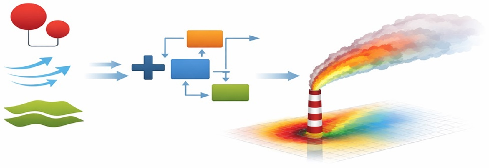
As mentioned above, besides the research and practical applications, one of the purposes of this model is to be used for teaching activities. Thus, it has been structured into several work areas so that students can more easily observe the data flow, the functions used, and the results obtained. The model consists of the following areas: data input, distance rasters, stability class, plume rise, dispersion coefficients, and concentration calculation (Figure 1). Even if the work process is divided into several work areas, their execution will be carried out in a single process. Each work area is detailed below.

The QGIS-based model was developed and all simulations were performed using QGIS version 3.34.7, GRASS GIS version 8.3.2 and GDAL version 3.9.0. The Manchester University Gaussian Plume Model and the Vasdev Gaussian Plume Model were executed using Python version 3.12.3.

2.2. Data Input and Preprocessing

The model starts with data input work area. The model input parameters are described in

Table 1. The model input parameters.

Parameter Name	Description
Project CRS	Coordinate Reference System (CRS) of the project, defined according to national or regional standards
Stack coordinates	Geographic coordinates of the emission source defined in the selected Project CRS
Stack height [m]	Physical height of the stack above ground level in meters
Stack diameter [m]	Inner diameter of the stack outlet
DEM	Digital Elevation Model covering at least the maximum dispersion distance
Area type	Classification of the study area as rural or urban
Mass flow [g/s]	Pollutant emission rate expressed in grams per second
Gas exit velocity [m/s]	Exit velocity of the emitted gas at the stack outlet
Air temperature [C_degree]	Ambient air temperature measured at 2 m above ground level in Celsius degrees
Gas exit temperature [C_degree]	Temperature of the exhaust gas at the stack outlet
Wind speed [m/s]	Wind speed measured at 10 m above ground level
Wind direction [degree]	Wind direction measured at 10 m above ground level in degrees
Solar radiation [W/m2]	Instant solar radiation in Watt/squared meter
Max. dispersion distance [m]	Maximum downwind distance considered in the dispersion calculations
Resolution [m]	Spatial resolution of the output raster datasets

.

To avoid any ambiguity regarding unit consistency across model inputs, intermediate products, and outputs,

Table 2. Summary of units used in the dispersion modeling workflow.

Parameter	Unit
Emission rate	g/s
Wind speed	m/s
Stack height/distances	m
Solar radiation	W/m2
QGIS model concentration output	µg/m3
Reference model concentration output	g/m3
Converted reference concentration output	µg/m3

summarizes the units used throughout the dispersion modeling workflow.

All reference model outputs originally expressed in g/m³ were converted to µg·m⁻³ prior to raster comparison.

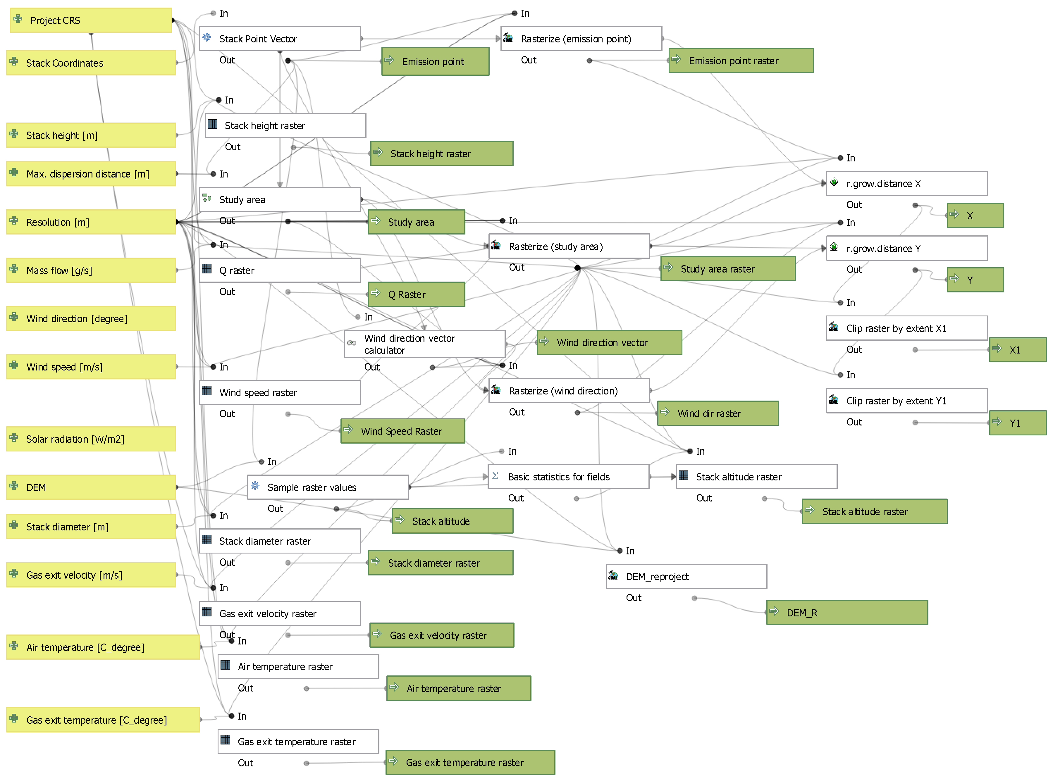
Some of these input parameters required additional transformations to be used with the QGIS model designer available functions. For example, since the QGIS Raster Calculator function only uses raster inputs, the parameters chimney altitude, chimney height, study area, mass flow, wind speed, and wind direction were transformed from float numerical inputs into constant-value rasters, as can be seen in Figure 2.

Using the user inputs, the chimney coordinates are first converted into a point vector layer, which is subsequently rasterized to produce the spatial representation of the emission location. The stack height input value is combined with terrain elevation extracted from the Digital Elevation Model (DEM), using a raster sampling procedure, to derive the absolute chimney altitude. This altitude raster is used to determine the effective release height used in subsequent plume rise and dispersion calculations.

The modelling domain is defined by buffering the emission source by the maximum dispersion distance. The resulting polygon is rasterized to produce a study-area mask, ensuring that all subsequent computations are spatially constrained to the domain of interest. This approach minimizes computational overhead and ensures spatial coherence among the derived rasters.

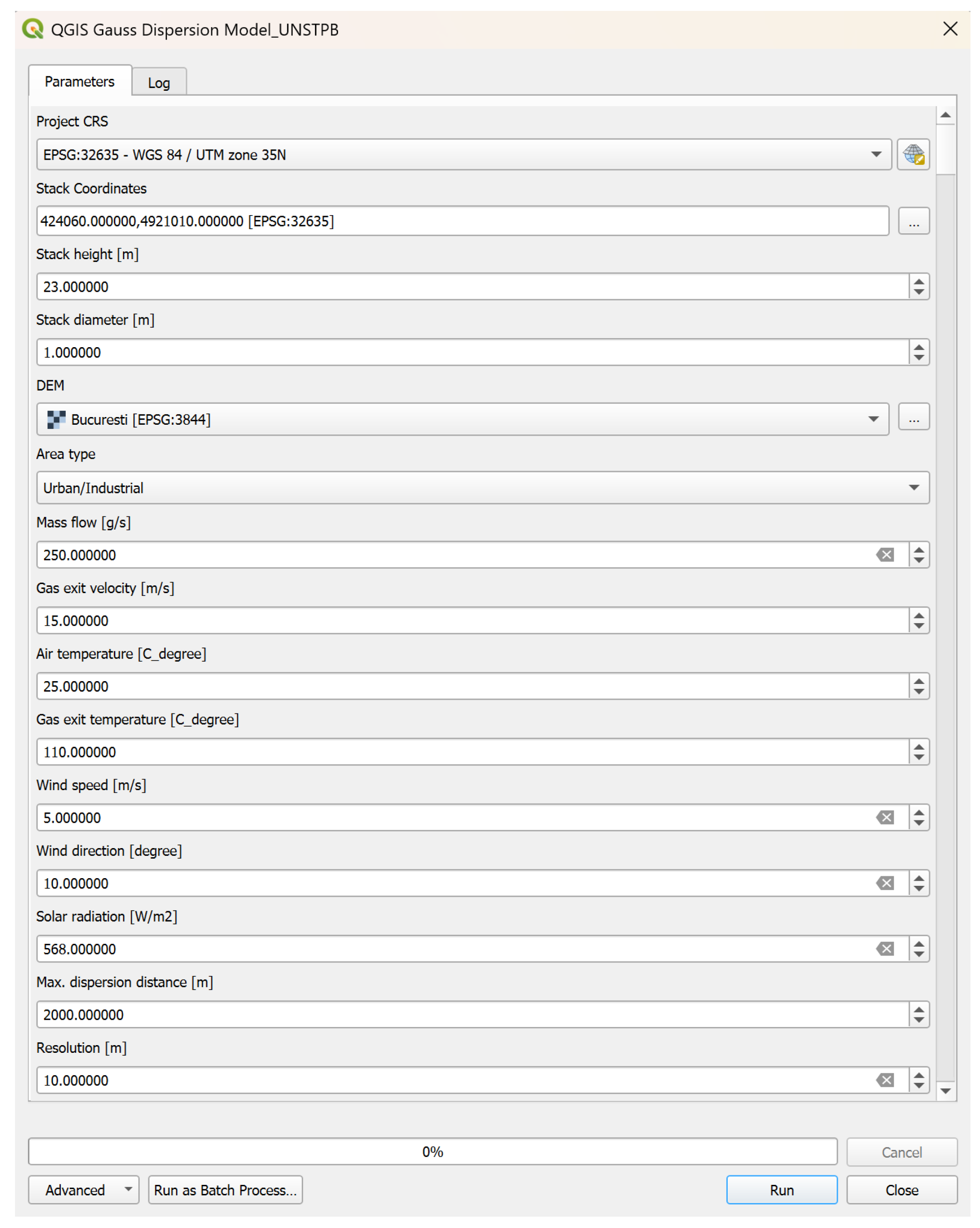
The data input Graphical User Interface (GUI) of the model, shown in Figure 3, is simple and intuitive, allowing users to easily enter the required input parameters and select the desired model outputs prior to execution.

Meteorological variables are transformed from scalar inputs into spatially explicit raster fields. Wind direction value provided by user in a meteorological format is converted to downwind azimuths using a trigonometric transformation compatible with the QGIS coordinate system. The resulting components are rasterized to generate the wind-direction field. Wind speed is similarly converted to a continuous raster layer. These meteorological rasters form the basis for modelling advection and the directional influence on plume transport.

The pollutant mass flow rate is distributed spatially by rasterizing the emission source into the modelling domain, yielding the Q-raster. This raster functions as the source term in the Gaussian dispersion equation and is subsequently combined with meteorological and topographic layers during concentration calculations.

The DEM is used to account for variations in ground elevation across the study area. For the model testing presented in this study, a DEM with 10 m spatial resolution, obtained from the Romanian National Agency for Cadastre and Land Registration (ANCPI), was used. Given the predominantly flat topography of the study area, this resolution is considered sufficient to represent local elevation variability and its influence on effective stack height. While the model supports DEMs of different resolutions, correlating the DEM resolution with the model input resolution ensures spatial consistency and avoids unnecessary resampling effects.

The extracted terrain height at the stack location, combined with the chimney height, yields the final raster layer describing the chimney altitude above sea level. This variable is essential for determining the effective plume rise, particularly in complex terrain.

All intermediate rasters, including emission point, chimney altitude, chimney height, wind speed, wind direction, and emission rate, are automatically resampled to a common resolution defined by the user. The harmonized set of rasters constitutes the complete geospatial input dataset required for the GP model.

2.3. Distance Raster Computation

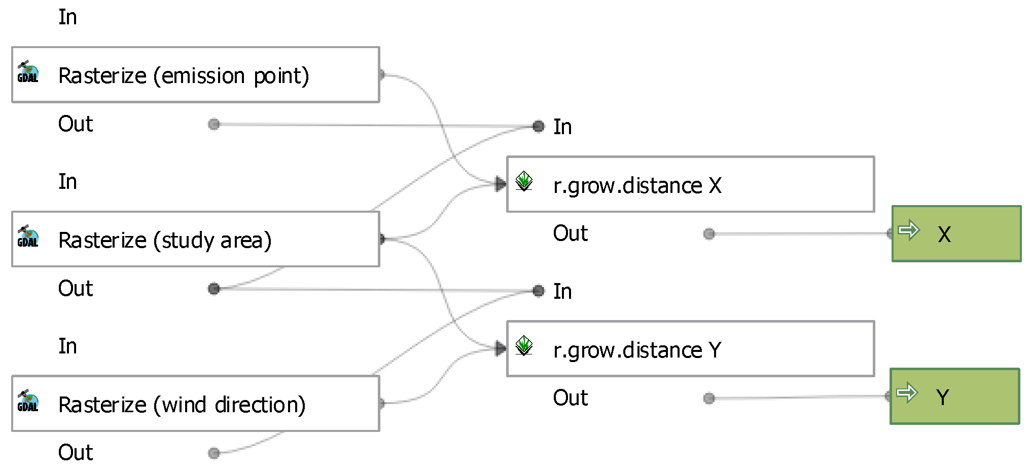
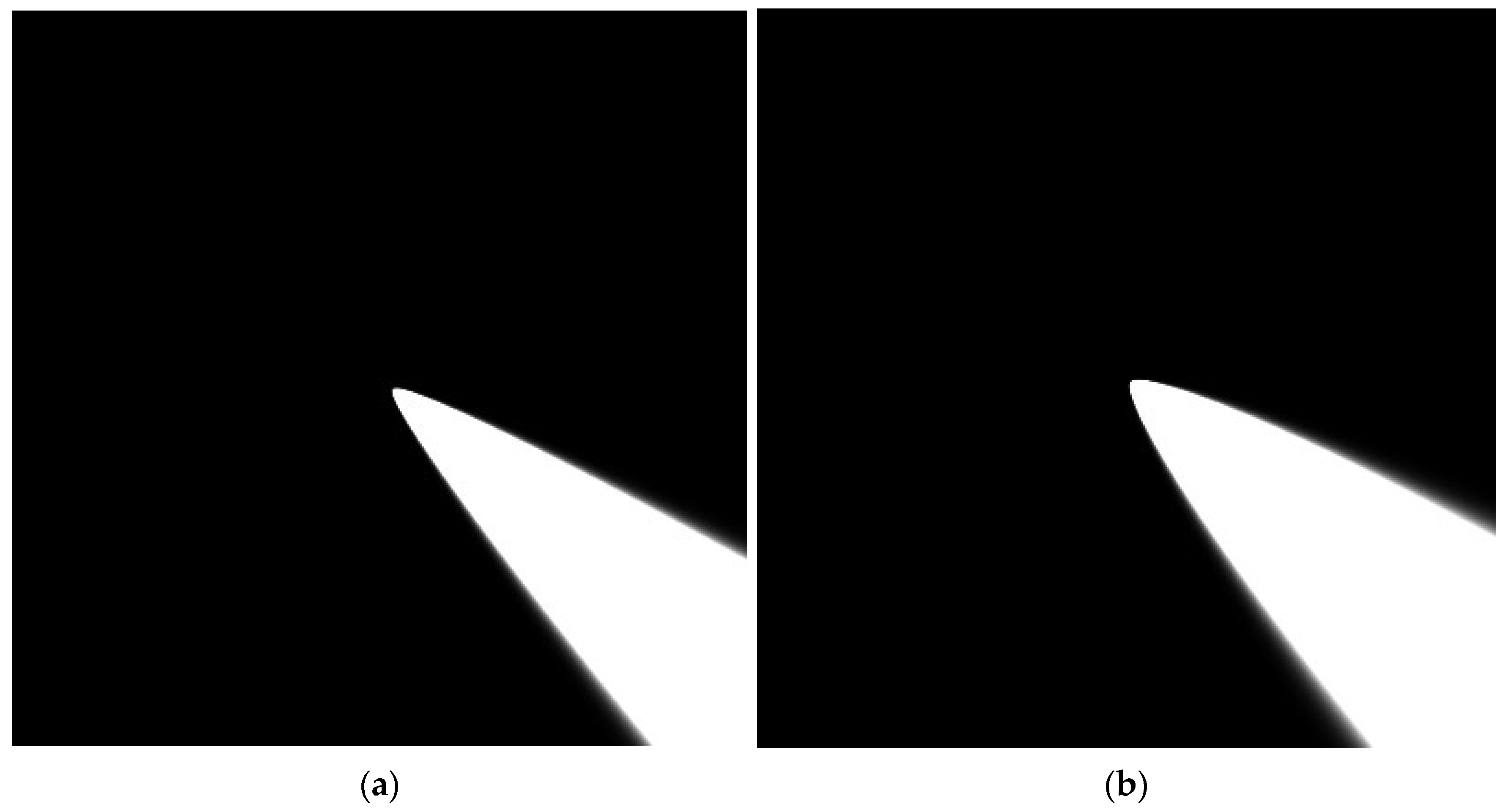
Using the resulting emission point, study area and wind direction rasters the next step was to create two distance rasters on the x-axis and y-axis using the GRASS tool “r.grow.distance”. The GRASS tool was set to calculate the Euclidian distances from the chimney location in all directions for the x-axis and in direction of wind for the y-axis for the entire study area (Figure 4).

2.4. Atmospheric Stability Classification

The next work area is used to assess the atmospheric stability. Atmospheric stability plays a fundamental role in determining the dispersion and dilution of pollutants in the lower atmosphere. One of the most widely used frameworks for characterizing stability conditions is the Pasquill stability classification, introduced in 1961 [30]. This system categorizes stability into six classes (A through F) based on meteorological parameters such as solar radiation, cloud cover, wind speed, and near-surface temperature gradients, all of which influence the degree of vertical and horizontal air mixing. Classes range from A (very unstable) to F (very stable) and serve as a core input for GP dispersion models used in environmental impact assessments [11,31].

Atmospheric stability classes characterize the intensity of turbulence and mixing in the lower atmosphere and strongly influence pollutant dispersion. Unstable conditions (Classes A–C), typically associated with daytime solar heating, promote enhanced vertical and horizontal mixing and rapid dilution of pollutants, whereas neutral conditions (Class D) limit buoyant turbulence and result in narrower plumes. Stable conditions (Classes E and F), common during nighttime under light winds, suppress vertical motion and lead to reduced dispersion and elevated near-surface concentrations. The Pasquill—Gifford stability classes remain a cornerstone in atmospheric dispersion modeling due to their simplicity, empirical grounding, and compatibility with regulatory modeling frameworks.

The QGIS model uses these stability classes to assess the impact of point sources. Atmospheric stability was determined using a slightly modified Pasquill–Gifford classification in which solar radiation is introduced as a numeric input together with wind speed. This approach was adopted to preserve the physical interpretation of convective forcing underlying the original Pasquill scheme, while avoiding subjective qualitative descriptors such as cloud cover or insolation categories. Solar radiation represents a direct and measurable proxy for surface heating and turbulence generation during daytime conditions, allowing stability classes to be assigned in a reproducible and transparent manner. The modified classification therefore maintains consistency with classical Pasquill–Gifford concepts while improving usability within a GIS-based modeling framework [11,13,17,27,32,33].

The modified Pasquill–Gifford stability classification presented in

Table 3. The modified Pasquill—Gifford stability classification table.

Pasquill Stability Class	Solar Radiation [W/m2]	10 m Wind Speed [m/s]
A—very unstable	≥700	<3
	≥300 and <700	<2
B—moderately unstable	<300	<2
	≥300 and <700	≥2 and <4
	≥700	≥3 and <5
C—slightly unstable	<300	≥2 and <5
	≥300 and <700	≥4 and <6
	≥700	≥5
D—neutral	<300	≥5
	≥300 and <700	≥6
E—slightly stable	0	<3
F—stable	0	≥3 and <5

is applied primarily to daytime conditions, where atmospheric stability is driven by solar heating. Solar radiation values greater than zero represent daytime convective forcing, while a value of 0 W/m² corresponds to nighttime or fully overcast conditions, for which stability classes (E and F) are assigned based solely on wind speed. This formulation allows a consistent treatment of both daytime and nighttime conditions within a single, numerically defined framework.

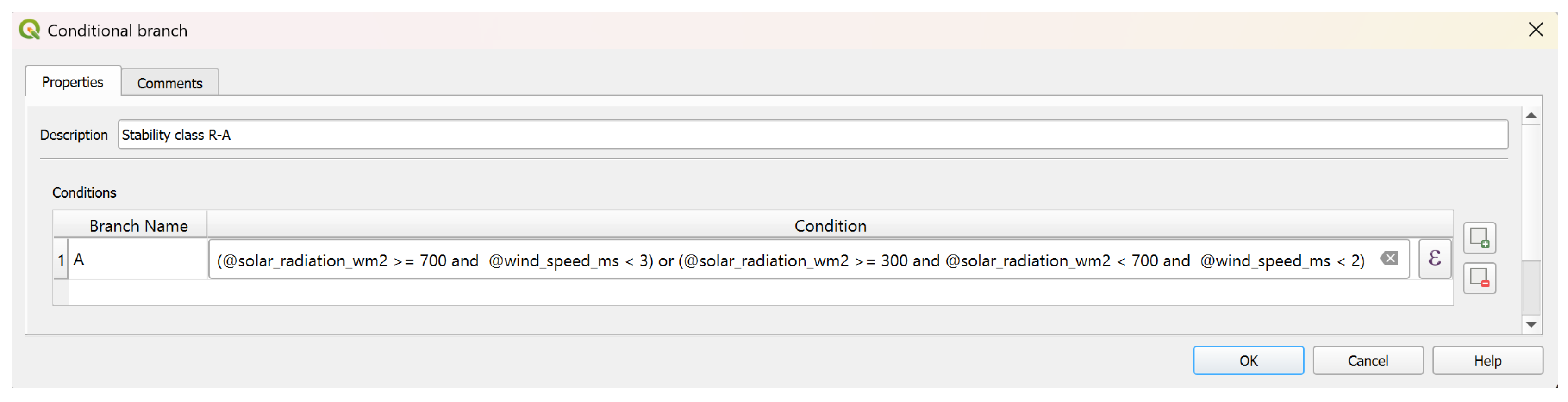
To determine the correct atmospheric stability class, based on data inputs, a conditional branch was used for each class (from A to F) by setting the condition based on the above-mentioned parameters. One example is shown in Figure 5.

2.5. Dispersion Coefficient Calculation

After the determination of the correct atmospheric stability class the next step was to compute the dispersion coefficients based on the Briggs’ formulas for each class. Briggs parameters for atmospheric dispersion coefficients for open/rural sites and urban/industrial sites are presented in

Table 4. Briggs parameters used to determine the dispersion coefficients.

Stability Class	Open/Rural Sites		Urban/Industrial Sites
	${\mathit{\sigma }}_{\mathit{y}}\left[\mathbf{m}\right]$	${\mathit{\sigma }}_{\mathit{z}}\left[\mathbf{m}\right]$	${\mathit{\sigma }}_{\mathit{y}}\left[\mathbf{m}\right]$	${\mathit{\sigma }}_{\mathit{z}}\left[\mathbf{m}\right]$
A	${\displaystyle \frac{0.22x}{\sqrt{1+0.0001x}}}$	$0.20x$	${\displaystyle \frac{0.32x}{\sqrt{1+0.0004x}}}$	$0.24x\sqrt{1+0.001x}$
B	${\displaystyle \frac{0.16x}{\sqrt{1+0.0001x}}}$	$0.12x$
C	${\displaystyle \frac{0.11x}{\sqrt{1+0.0001x}}}$	${\displaystyle \frac{0.08x}{\sqrt{1+0.0002x}}}$	${\displaystyle \frac{0.22x}{\sqrt{1+0.0004x}}}$	$0.20x$
D	${\displaystyle \frac{0.08x}{\sqrt{1+0.0001x}}}$	${\displaystyle \frac{0.06x}{\sqrt{1+0.0015x}}}$	${\displaystyle \frac{0.16x}{\sqrt{1+0.0004x}}}$	${\displaystyle \frac{0.14x}{\sqrt{1+0.0003x}}}$
E	${\displaystyle \frac{0.06x}{\sqrt{1+0.0001x}}}$	${\displaystyle \frac{0.03x}{1+0.0003x}}$	${\displaystyle \frac{0.11x}{\sqrt{1+0.0004x}}}$	${\displaystyle \frac{0.08x}{\sqrt{1+0.0015x}}}$
F	${\displaystyle \frac{0.04x}{\sqrt{1+0.0001x}}}$	${\displaystyle \frac{0.016x}{1+0.0003x}}$

.

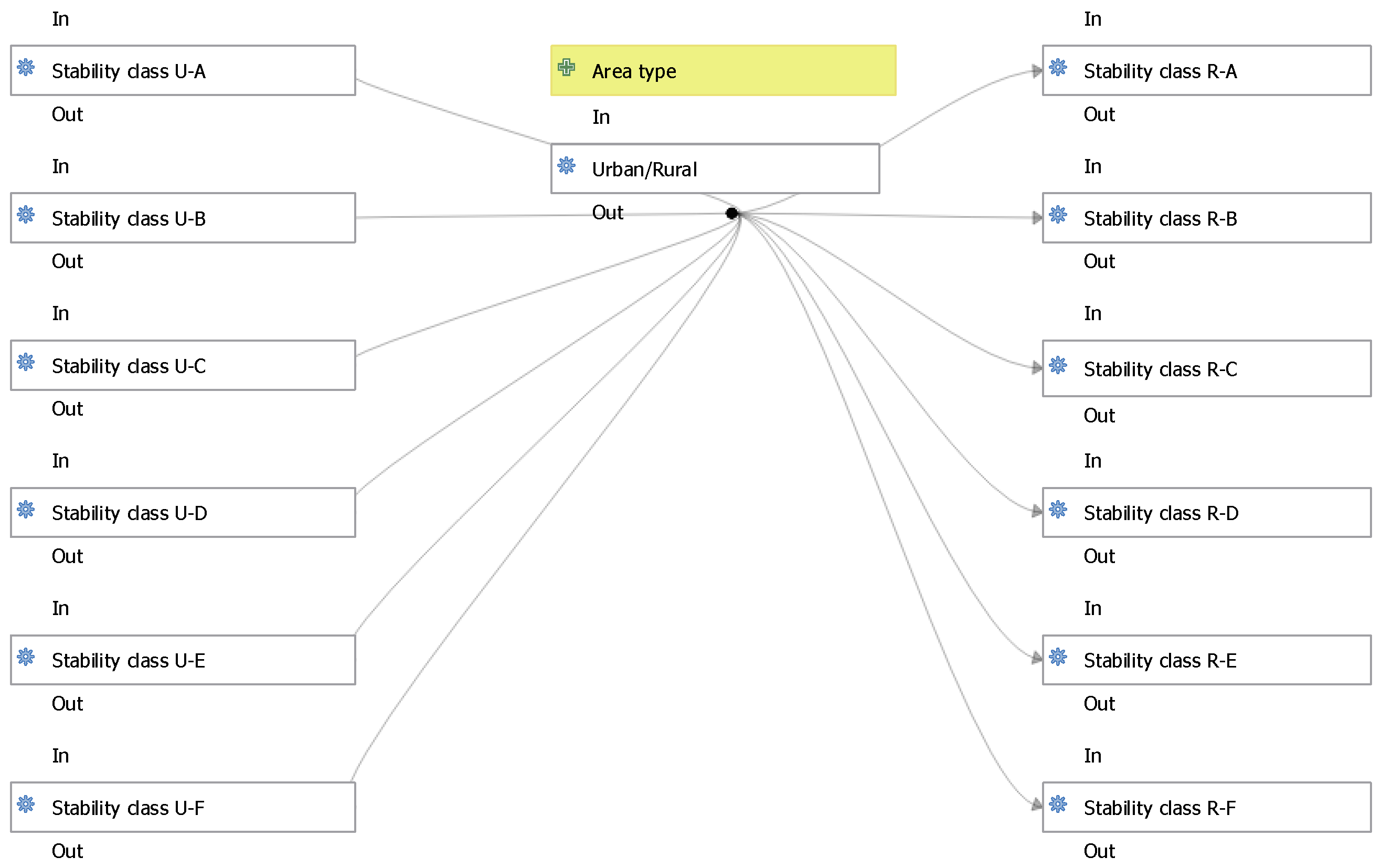
To ensure that the QGIS model performs only the calculations required based on the user-selected area type and the previously determined stability class, a conditional structure was created, as shown in Figure 6. This approach also improves efficiency by enabling the model to run faster and avoid unnecessary computations.

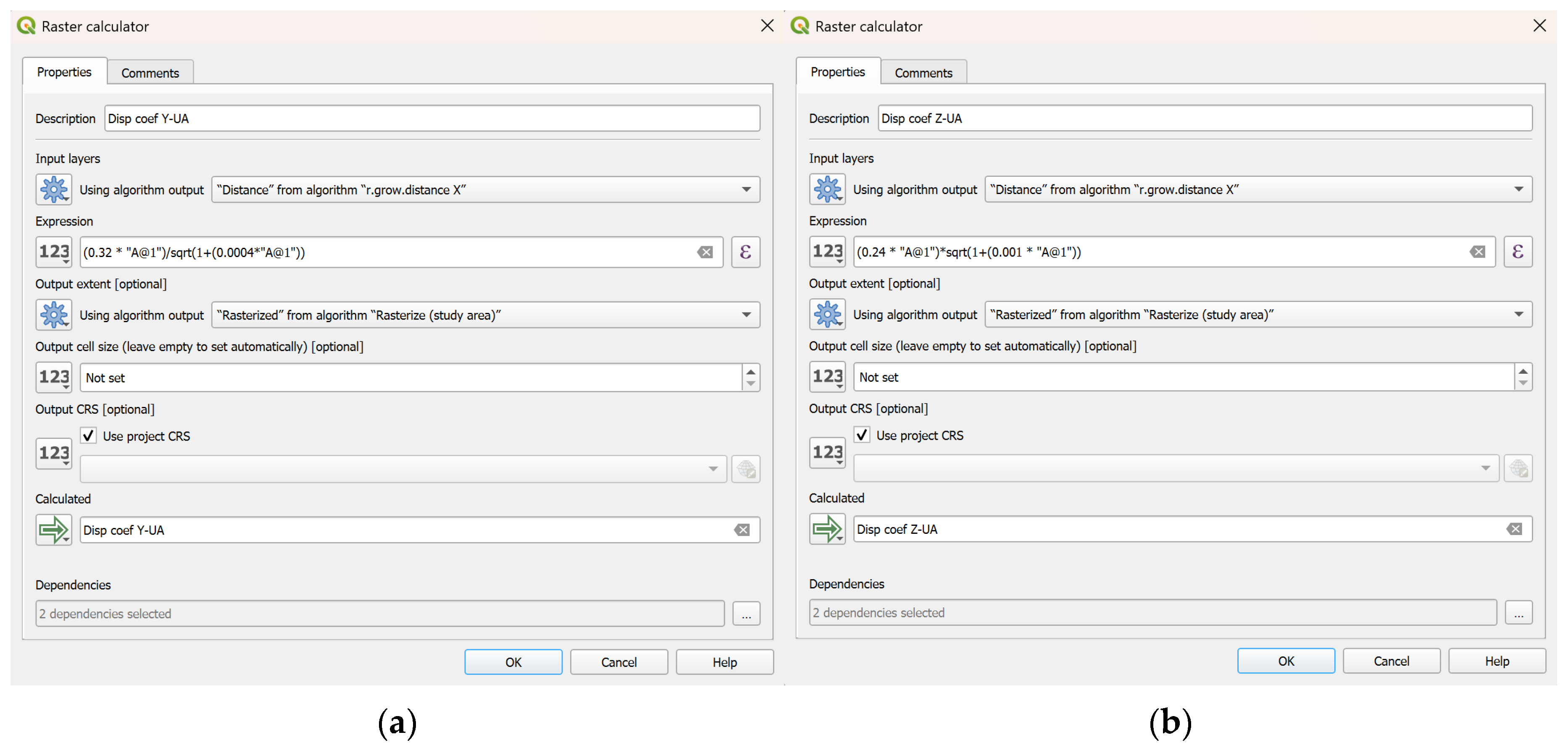
For each site type and for each stability class the ${\sigma }_y$ and ${\sigma }_z$ dispersion coefficients were calculated by using the Raster Calculator function from QGIS setting as inputs the X distance raster for downwind distance and study area raster for the output extent. The dispersion coefficients will show how pollutant plumes spread horizontally (${\sigma }_y$) and vertically (${\sigma }_z$) with downwind distance (x) depending on the atmospheric stability class. One example is shown in Figure 7a,b.

2.6. Plume Rise Estimation

The next computational area is used to determine the effective release height of the emitted pollutant, denoted as $H$, as the sum of the physical stack height ($h$) and the plume rise ($∆h$).

$$H=h+∆h$$

(2)

The physical stack height is a user input parameter, while the plume rise is calculated based on the user inputs. The plume rise is computed using the classical Briggs formulas depending on atmospheric stability: buoyancy-driven Formula (3) for class A, B and F, momentum-dominated Formula (4) for class D and the maximum value of both equations for C and E classes.

$$∆h=2.6{\displaystyle \frac{{\left(g{D}^2{v}_e\frac{T_s-T_a}{4T_a}\right)}^{1/3}}{u\left(h\right)}}$$

(3)

where $g$ is the acceleration due to gravity (9.81 m/s²), $D$ is the stack diameter (m), $v_e$ is stack exit velocity (m/s), $T_s$ is stack gas temperature (K), $T_a$ is ambient air temperature (K) and $u\left(h\right)$ is the wind speed at stack height (m/s).

$$∆h=1.6D{\left({\displaystyle \frac{v_e}{u\left(h\right)}}\right)}^{0.4}$$

(4)

where $D$ is the stack diameter (m), $v_e$ is the pollutant exit velocity at the stack top (m/s) and $u\left(h\right)$ is the wind speed at stack height (m/s).

This approach is widely accepted in regulatory dispersion modeling and provides a physically consistent estimate that does not require thermodynamic plume buoyancy or detailed atmospheric stability information.

The wind speed at the stack height $u\left(h\right)$ is calculated from the measured 10-m wind speed $u_{10}$ and stack height ($h$), using the standard power law wind profile:

$$u(\mathrm{h})=u_{10}{\left({\displaystyle \frac{\mathrm{h}}{10}}\right)}^{\alpha }$$

(5)

where the exponent $\alpha$ depends on surface roughness, with typical values of $\alpha = 0.14$ for rural conditions and $\alpha =0.20$ for urban environments. This adjustment accounts for the vertical variation in wind speed, which directly influences the plume’s momentum and buoyancy behavior.

2.7. Ground-Level Concentration Calculation

Finally, all model parameters are introduced into the GP Equation (1). For computational implementation, the Gaussian dispersion formulation was decomposed into four analytical components, as illustrated in Figure 8. Each term of the equation is evaluated separately using the QGIS embedded Raster Calculator to represent the individual physical processes governing plume behavior.

Computing the four analytical components of the GP equation (T1–T4) separately offers several methodological advantages. First, it enables a clear physical interpretation of each contribution to the final concentration field, with T1 defining the centerline concentration scaling, T2 representing lateral turbulent spreading, T3 describing vertical dispersion around the effective release height, and T4 accounting for ground reflection. Second, the explicit separation of terms improves numerical transparency by allowing each process to be evaluated, visualized, and validated independently within the raster-based environment. Third, this modular structure facilitates diagnostic analyses, making it possible to assess the relative influence of transport, dispersion, and surface interaction mechanisms on modeled concentrations. Component-wise implementation enhances model flexibility, as individual terms or parameterizations can be refined or replaced without altering the overall computational framework, thereby supporting future model development and sensitivity analyses.

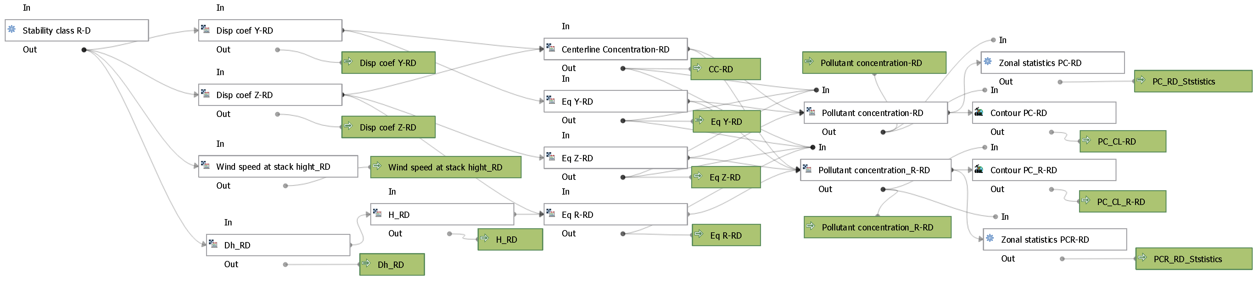
A complete conditional branch of the QGIS-based dispersion model, corresponding to open (rural) terrain and Pasquill stability class D, is presented in Figure 9. Each computational step in the workflow generates intermediate raster outputs, displayed as green boxes, which represent spatially explicit evaluations of the individual analytical components of the GP equation. The intermediate results are combined, resulting in concentration components associated with plume dispersion (centerline concentration, lateral and vertical dispersion and ground reflection).

These components are finally assembled into continuous pollutant concentration fields representing the spatial distribution of ground-level concentrations for stability class D under rural conditions, both with and without accounting for plume reflection at the surface. The resulting rasters constitute the primary outputs of the model and provide the basis for subsequent visualization, statistical analysis, and comparative assessment. To enhance the interpretation of pollution hotspots, spatial patterns, and plume geometry, contour-line (isopleth) representations were also incorporated into the modeling workflow.

To verify the correctness of the embedded QGIS Raster Calculator operations, all computations were independently replicated using the GDAL Raster Calculator. Both implementations produced identical results, confirming the numerical consistency and reliability of the modeling framework.

2.8. Model Assumptions and Applicability

As mentioned previously, the resulting QGIS model was used for testing purposes to assess the CO₂ dispersion from the TPP located at Politehnica Bucharest campus.

Carbon dioxide was selected as the test pollutant due to its inert behavior at the local scale and well-characterized emission rates. Although CO₂ is not commonly used for local health exposure assessment, its use in this study allows the dispersion behavior of the Gaussian plume formulation to be examined without additional complexity, supporting methodological demonstration and teaching purposes. However, the proposed GIS-based model is directly applicable to health-relevant pollutants such as PM_2.5, NO₂, SO₂ when appropriate emission data are available.

The Gaussian plume formulation implemented in this study assumes steady-state meteorological conditions, homogeneous turbulence, constant emission rates, and horizontally uniform wind fields. The model is applicable primarily under non-calm wind conditions and for downwind distances beyond the immediate near-field, where building downwash and complex flow effects are negligible. Under calm winds, strong atmospheric stratification, complex urban geometries, or highly variable meteorological conditions, the Gaussian plume approach may become unreliable.

2.9. Study Area

The study area comprises the campus and the surrounding areas of the Politehnica Bucharest, located in the western sector of Bucharest, Romania. The area is situated on the Romanian Plain and is characterized by predominantly flat terrain with minimal elevation variation, allowing terrain effects on airflow to be considered negligible at the local scale.

The campus exhibits a mixed urban land-use pattern, including academic buildings, residential structures, road infrastructure, and green spaces, resulting in heterogeneous surface roughness that influences local wind flow and pollutant dispersion. Climatically, the region experiences a temperate continental climate with distinct seasonal variability, characterized by warm summers, cold winters, and variable atmospheric stability conditions throughout the year.

These characteristics make the study area representative of an urban environment suitable for the application of GP dispersion modeling.

The selected campus-scale configuration is used to demonstrate the proposed QGIS workflow and to enable controlled intercomparison of plume formulations; the implementation is general and can be applied to other point sources by providing the corresponding emission, meteorological, and terrain inputs.

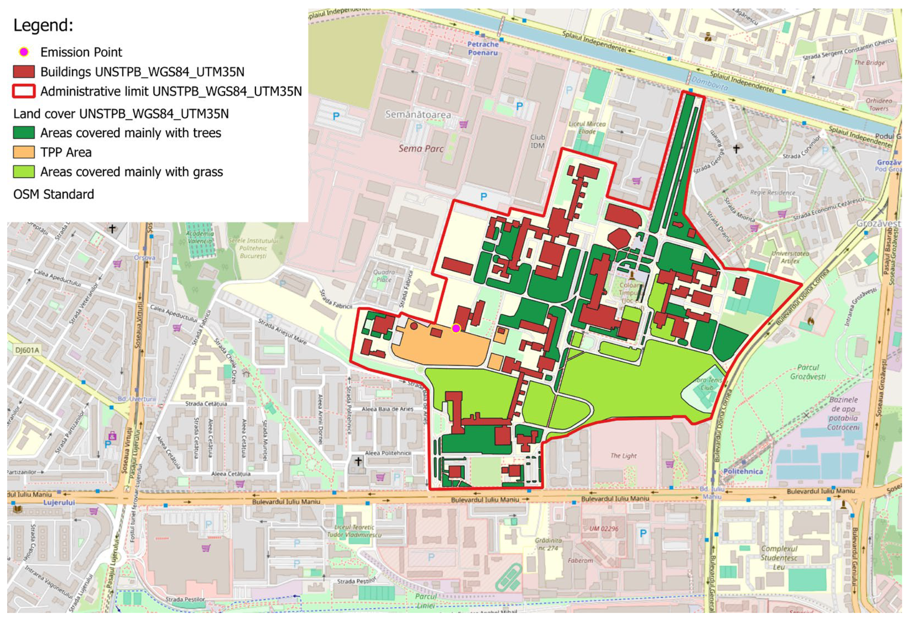
To facilitate the identification of areas with maximum pollutant concentrations within the university campus, vector layers representing buildings and vegetation were created. Also, an OpenStreetMap (OSM) standard raster was added to provide an overview of surrounding area.

These layers are not generated by the dispersion model itself but are incorporated as auxiliary spatial data to support the interpretation of results. Their inclusion enables a clearer spatial context for the modeled concentration fields, allowing hotspots to be related to terrain altitude variation, built structures and green areas within the study domain. A map with the study area and above-mentioned layers is presented in Figure 10.

3. Results

The model was tested using calculated CO₂ emission rates based on instant natural gas consumption of the TPP and real meteorological data corresponding to an afternoon period in the latter part of September 2025. The input parameters used to generate the results presented below are summarized in

Table 5. The input parameters used for simulation.

Parameter Name	Value
Project CRS	EPSG:32635—WGS84/UTM zone 35N
Stack coordinates	424060, 4921010
Stack height [m]	23
Stack diameter [m]	1
Area type	Urban
Mass flow [g/s]	212
Gas exit velocity [m/s]	15
Air temperature [°C]	22
Gas exit temperature [°C]	110
Wind speed [m/s]	6
Wind direction [°]	310
Solar radiation [W/m2]	568
Max. dispersion distance [m]	2000
Resolution [m]	10

.

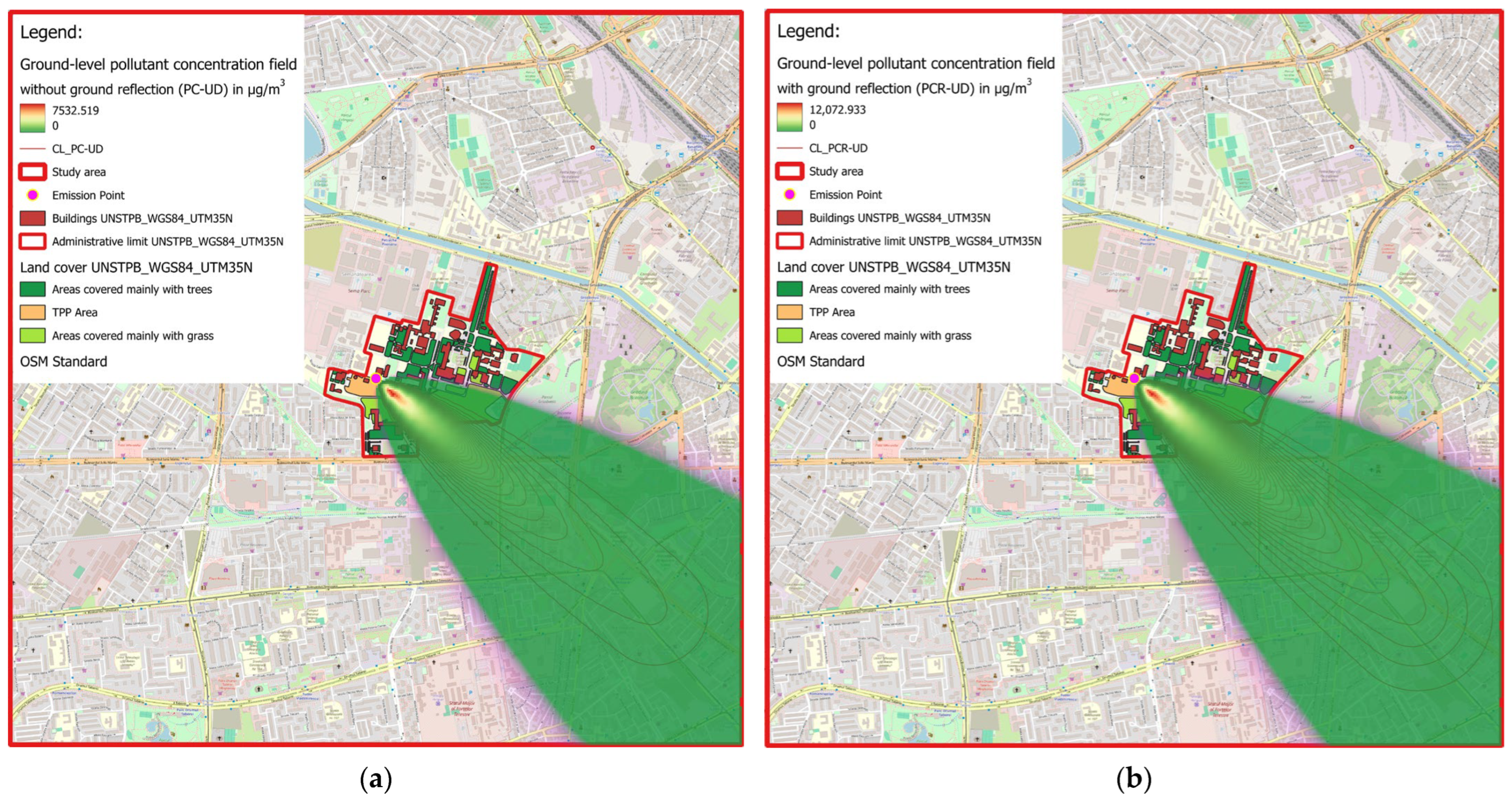
The QGIS-based model produced two raster outputs representing ground-level concentrations for the case study: one without ground reflection (PC-UD) and one including the image source term (PCR-UD) presented in Figure 11.

For visualization purposes, both rasters were symbolized using a green-to-red color gradient and classified into eight equal intervals. Also, contour line with a 50 µg/m³ interval were added to facilitate visualization of the dispersion plum.

Figure 11a presents the concentration field obtained without accounting for ground reflection, serving as a baseline representation of the direct plume contribution to surface-level concentrations. In contrast, Figure 11b illustrates the results obtained when ground reflection is included, capturing the additional pollutant contribution associated with surface-induced plume rebound, which is known to enhance near-ground concentration maxima and increase the spatial extent of elevated concentration levels.

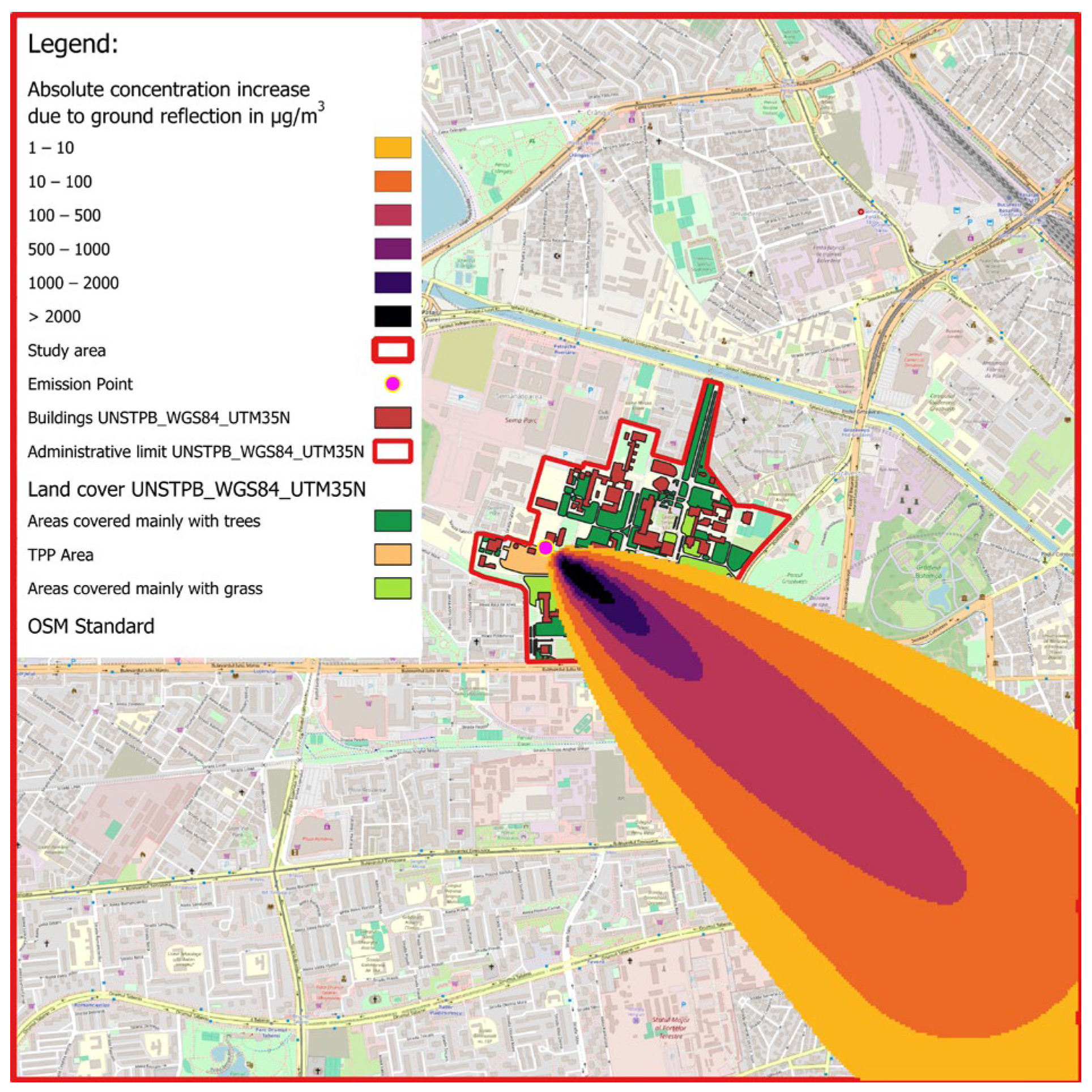
To highlight the visual differences between the modeled ground-level concentration fields (PCR-UD and PC-UD) an absolute difference map was created. Figure 12 illustrates this difference, isolating the effect of the ground reflection boundary condition. The difference field is strictly positive, confirming that inclusion of ground reflection systematically increases near-surface concentrations across the domain. The strongest amplification occurs in the near-field region downwind of the source, where reflection enhances plume confinement and vertical concentration gradients. Differences decrease progressively with distance from the source but remain spatially coherent along the plume centerline, indicating that ground reflection influences not only peak values but also the broader spatial extent of elevated concentrations.

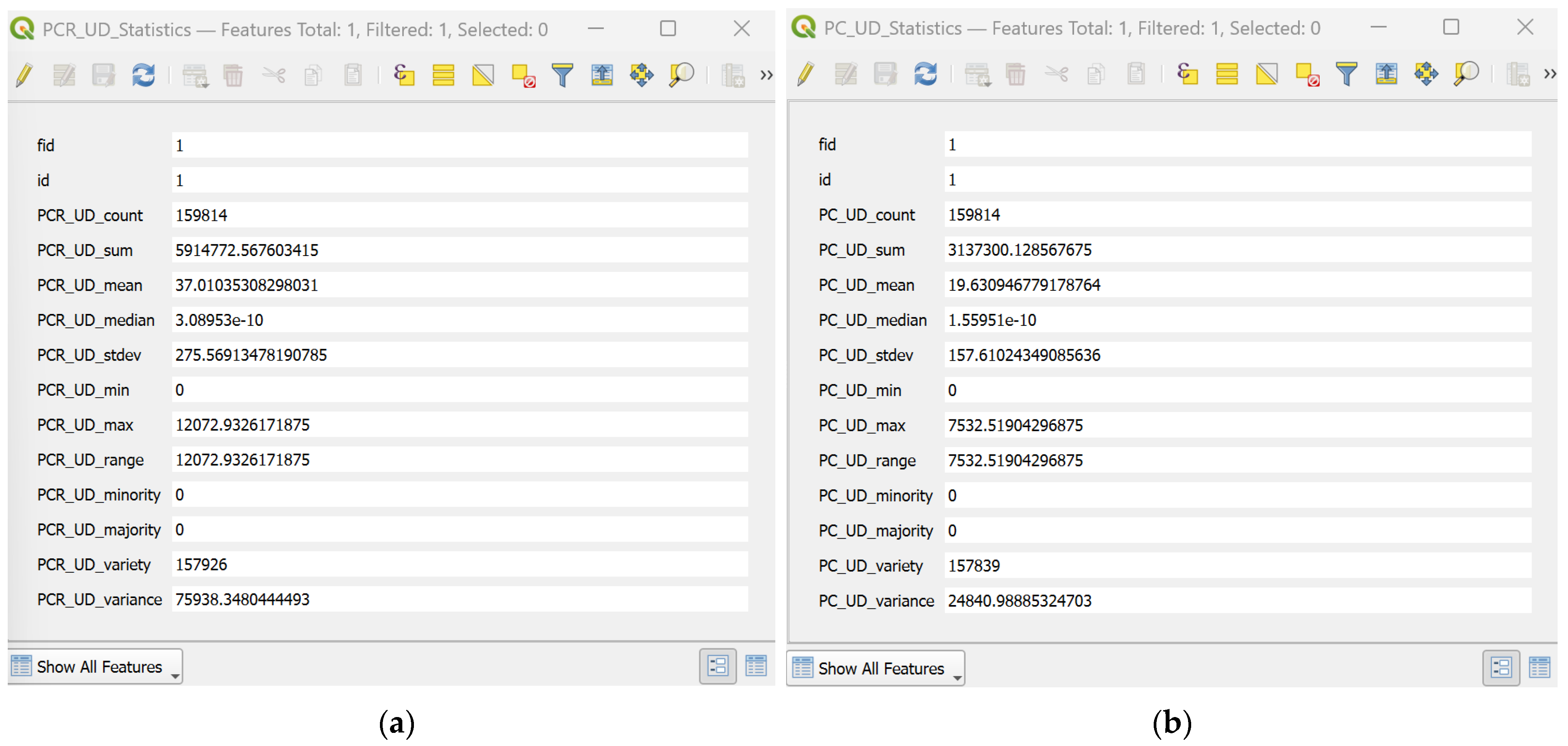
Descriptive statistics were extracted from the modeled concentration rasters to characterize the spatial distribution of pollutant levels. The results presented in Figure 13 and

Table 6. Percentile statistics (5th, 25th, 75th, and 95th percentiles) of the modeled ground-level pollutant concentration rasters.

Concentration Raster	P5 (µg/m3)	P25 (µg/m3)	P75 (µg/m3)	P95 (µg/m3)
PC-UD	3.51 × 10−12	3.91 × 10−13	1.38 × 10−4	80.628
PCR-UD	6.998 × 10−12	7.79 × 10−13	2.72 × 10−4	159.845

indicate a highly skewed distribution, with low background concentrations across most of the domain and localized maxima in the vicinity of the emission source.

The dispersion results without ground reflection show that CO₂ ground-level concentrations are generally very low across most of the domain, as indicated by near-zero median and lower quantile values. Only a limited portion of the area exhibits elevated concentrations, reflected in the relatively high maximum value (7532.519 µg/m³) and a 95th percentile of 80.628 µg/m³. The mean concentration (19.631 µg/m³) and the large standard deviation (157.61 µg/m³) confirm a strongly skewed distribution, characteristic of a narrow, high-intensity plume core surrounded by extensive low-concentration regions. The raster represents a typical Gaussian dispersion pattern where most of the modeled area experiences negligible impact, while the plume centerline contains the dominant concentration values.

The inclusion of the ground reflection component in the Gaussian dispersion simulation produced a marked increase in modeled near-surface concentrations. Maximum CO₂ concentrations increased from 7532.519 to 12,072.933 µg/m³ (+60.3%), while the domain-wide mean concentration increased from 19.63 to 37.01 µg/m³ (+88.5%). Although lower quantiles remained close to zero, reflecting the dominance of low-concentration areas across the domain, upper quantiles evidenced substantial increases. The 95th percentile increased from 80.628 to 159.845 µg/m³, indicating a strong amplification of high-exposure zones. This behavior aligns with the theoretical expectation that introducing a reflective boundary at the ground surface enhances the downwind mass flux and increases near-ground pollutant accumulation.

To validate the result, two open-source Python models were used: the Manchester University Gaussian Plume Model (MU-GP) [27,28] and a classical Gaussian Plume Model from Vasdev Github repository (VGP) [29]. Both reference models were run on a regular grid of 10 m resolution and 4 km × 4 km extent centered on the stack, matching the QGIS domain and coordinate system. Resulting concentration fields (in g/m³) were converted to µg/m³ before comparison with the QGIS outputs. The raster results can be seen in Figure 14.

The MU-GP model is an implementation of the classical GP equation that incorporates internal parameterizations for atmospheric stability and dispersion coefficients (${\sigma }_y$ and ${\sigma }_z$). Its treatment of ground reflection is implicit: depending on the selected stability class and internal formulation, the model may partially account for reflected contributions, but it does not apply a full image source reflection term as in classical Briggs-based formulations. Consequently, its maximum predicted concentrations typically lie between those of a non-reflective plume and a fully reflective Gaussian model.

The VGP model adopts a classical steady-state Gaussian plume formulation with fixed power law parameterizations for lateral and vertical dispersion. Vertical reflection at the ground surface is explicitly represented through an image source technique, whereby a virtual plume mirrored below the ground plane is superimposed on the primary plume. This formulation enhances near-surface concentrations, particularly in the near-field, resulting in higher ground-level maxima and a more concentrated plume core compared to implementations that neglect ground reflection or apply more diffusive dispersion parameterizations.

The MU-GP model yields a maximum concentration of 8056.806 µg/m³, which lies between PC-UD and PCR-UD, indicating that reflection is partially, but not fully, represented based on the built-in stability and sigma formulations. The mean (85.677 µg/m³) is higher than in the user datasets, reflecting a somewhat narrower plume spread in the MU-GP sigma parameterization.

The VGP model produces the highest maximum concentration among the reference Gaussian plume formulations (12,618.130 µg/m³), closely approaching the PCR-UD peak. This behavior is expected, as the VGP formulation employs fixed power law dispersion coefficients combined with an explicit image source representation of ground reflection, which enhances near-field ground-level concentrations. Consequently, the VGP model predicts a more intense plume core while maintaining very low median and lower-percentile values across the domain.

A quantitative comparison of the four dispersion models (PC-UD, PCR-UD, MU-GP, and VGP) is provided in

Table 7. A quantitative comparison of the principal distributional metrics of the four models.

Metric	PC-UD (µg/m3)	PCR-UD (µg/m3)	MU-GP (µg/m3)	VGP (µg/m3)
Minimum	0.000	0.000	0.000	0.000
Maximum	7532.519	12,072.933	8056.806	12,618.130
Mean	19.631	37.010	85.677	52.750
Median	1.56 × 10−10	3.09 × 10−10	0.000	0.000
Std. Dev.	157.610	275.569	459.909	358.520
5th Percentile	3.51 × 10−12	6.998 × 10−12	0.000	0.000
95th Percentile	80.628	159.845	395.398	262.600

. The table summarizes the principal distributional metrics, including minimum, maximum, mean, median, standard deviation, and key percentiles, enabling a direct intercomparison of how ground reflection and model formulation influence near-surface pollutant concentrations.

To quantify model agreement several advanced statistical metrics were calculated in QGIS to quantify model agreement, including Root Mean Squared Error (RMSE), Mean Absolute Error (MAE), Mean Bias (MB), Normalized Mean Bias (NMB) and Pearson correlation (R). RMSE and MAE measure absolute and squared differences between paired model predictions. MB and NMB quantify systematic over or underprediction. R captures linear association across the spatial fields.

The advanced statistical comparison, presented in

Table 8. Advanced statistical metrics results.

Model Pair	RMSE (µg/m3)	MAE (µg/m3)	MB (µg/m3)	NMB (-)	R (-)
PC_UD vs. MU-GP	417.710	78.750	−66.107	−0.770	0.458
PC_UD vs. VGP	220.315	34.971	−33.169	−0.628	0.938
PCR_UD vs. MU-GP	404.332	75.788	−48.727	−0.568	0.499
PCR_UD vs. VGP	125.552	23.466	−15.790	−0.299	0.957

, confirms systematic differences among the four modeling approaches. The results show that the VGP model exhibits the strongest agreement with the user’s PCR-UD plume, as demonstrated by a high spatial correlation (R ≈ 0.957). This behavior is expected, as both formulations explicitly account for ground reflection through an image source approach, leading to similar plume geometry and near-surface concentration patterns.

In contrast, comparisons involving PC-UD reveal systematically lower agreement with the reference Gaussian plume models. The absence of an explicit ground reflection term in PC-UD produces a plume with reduced near-surface intensity and broader dispersion, resulting in weaker spatial agreement with MU-GP (R ≈ 0.458). Although a high correlation is observed between PC-UD and VGP (R ≈ 0.938), this primarily reflects similarity in plume geometry and spatial gradients rather than agreement in absolute concentration levels. These results highlight the dominant influence of ground reflection boundary conditions on plume morphology and spatial concentration patterns.

To assess the numerical consistency and reproducibility of the proposed model, multiple simulations were performed using identical input parameters. Repeated executions produced identical concentration fields and statistical outputs, confirming that the model behavior is deterministic and free from stochastic variability. This consistency verifies the stability of the computational workflow and demonstrates that the implementation yields reproducible results under fixed meteorological and emission conditions.

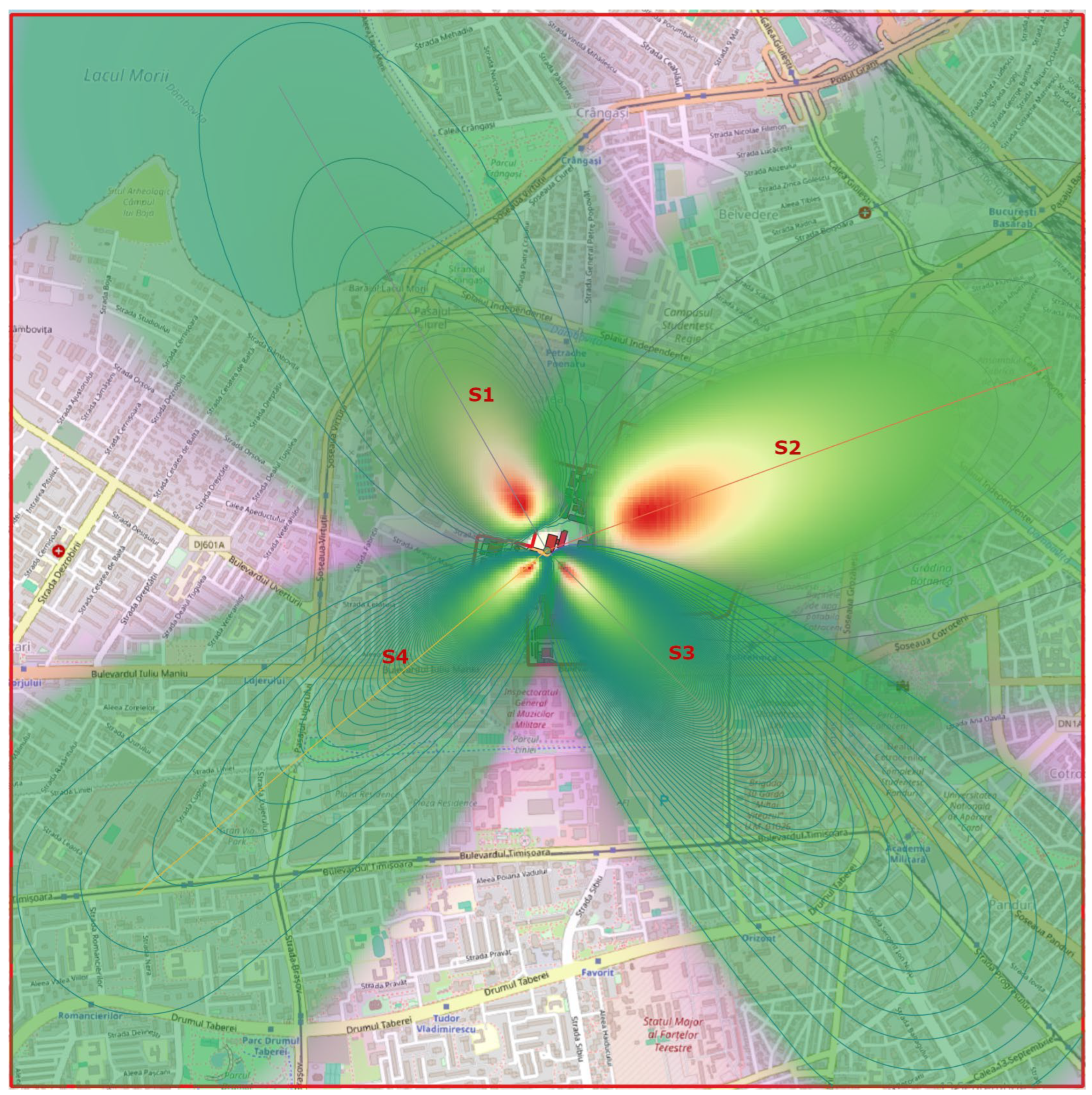
Also, the model was further tested through multiple simulations performed under different atmospheric stability classes by varying the corresponding meteorological input parameters. Four of these simulations (S1–S4) were overlayed and can be seen in Figure 15. The input parameters for the overlayed simulation are presented in

Table 9. The input parameters used for the overlayed simulations.

Input Parameter	Simulation S1	Simulation S2	Simulation S3	Simulation S4
Mass flow [g/s]	250	250	300	280
Gas exit velocity [m/s]	15	15	15	15
Air temperature [°C]	25	25	18	25
Gas exit temperature [°C]	110	110	110	110
Wind speed [m/s]	3	1	2	5
Wind direction [degree]	150	250	315	50
Solar radiation [W/m2]	568	568	1	298

.

All simulations were performed under non-calm conditions, with wind speeds representative of realistic atmospheric transport, ensuring the applicability of the Gaussian plume assumptions. The resulting concentration fields exhibited systematic and physically consistent variations in plume spread and peak values, with increased dispersion under unstable conditions and reduced spreading under stable regimes. This behavior confirms the model’s ability to appropriately represent stability-dependent dispersion processes.

4. Discussion

The comparison of the four Gaussian plume formulations highlights the influence of dispersion parameterizations and boundary condition treatments on ground-level pollutant concentrations. Although all models share the same physical basis, their behavior diverges in systematic and interpretable ways. The PCR-UD and VGP models produce the highest ground-level concentrations, reflecting their explicit treatment of the ground surface as a reflective boundary. This approach enhances near-surface concentrations by mirroring the plume below the ground plane, consistent with classical Gaussian plume theory. The VGP model yields the strongest near-field maxima, slightly exceeding those of PCR-UD, due to its fixed power law dispersion coefficients that generate a narrower plume core and reduced vertical dilution.

In contrast, the PC-UD model predicts substantially lower concentrations across the domain. The absence of explicit ground reflection allows greater vertical diffusion, resulting in weaker near-surface impacts and broader plume spread. This behavior aligns with theoretical expectations for non-reflective boundary conditions and underscores the dominant role of ground interaction in shaping surface concentration fields under neutral atmospheric conditions.

The MU-GP model occupies an intermediate position between reflective and non-reflective formulations. Its dispersion parameterization partially reproduces the effects of ground reflection, leading to moderate plume intensification without reaching the amplification observed in the VGP or PCR-UD models. Consequently, MU-GP peak concentrations lie between those of PC-UD and the explicitly reflective approaches. This intermediate behavior reflects differences in vertical dispersion treatment and is consistent with the known variability among Gaussian plume implementations.

The advanced statistical metrics reinforce these physical interpretations. Very high spatial correlation between PCR-UD and VGP confirms their shared reflective behavior and similar plume morphology. Comparisons involving PC-UD show reduced spatial agreement with the reference models, particularly with MU-GP, due to the absence of an explicit reflection term. Although PC-UD and VGP still exhibit a high correlation, this primarily reflects similarity in plume geometry and spatial gradients rather than agreement in absolute concentration levels. These findings emphasize that Pearson correlation captures spatial pattern coherence, whereas magnitude differences are more appropriately reflected by error and bias metrics.

From a GIS decision-support perspective, the choice of boundary condition (reflective versus non-reflective) directly influences the delineation of near-field high-concentration zones that may drive screening-level prioritization. Because the model outputs are spatial rasters, they can be readily combined with ancillary GIS layers (e.g., population distribution, schools, hospitals) to support preliminary exposure mapping and scenario comparison.

Despite the overall coherence of the results, several limitations should be acknowledged. All simulations are based on steady-state assumptions and neglect temporal variability in meteorological conditions, plume rise dynamics, chemical transformation, and deposition processes. Additionally, the dispersion parameterizations assume flat, homogeneous terrain, which may not fully represent real-world urban environments. The sensitivity of the predicted concentration fields to wind direction and stability classification further emphasizes the importance of accurate meteorological characterization in practical applications.

Atmospheric temperature inversions, which suppress vertical mixing, may lead to substantially higher near-surface concentrations than those predicted under neutral or unstable conditions. Although the present steady-state Gaussian plume framework can partially represent stable stratification through Pasquill stability classes, strong or persistent inversions may require more advanced modeling approaches. Consequently, results obtained under stable conditions should be interpreted conservatively, particularly for near-field exposure assessments.

Future research should extend this comparative framework to include unsteady or three-dimensional dispersion models, alternative stability schemes, and validation against field measurements.

Overall, the results demonstrate that Gaussian plume models can provide coherent and interpretable concentration fields, but their predictions depend strongly on the handling of ground reflection and dispersion coefficients. Understanding these structural differences is essential for selecting appropriate models in environmental impact assessments, regulatory analysis, and operational plume forecasting.

From a screening and regulatory preassessment perspective, these findings imply that Gaussian plume formulations lacking explicit ground reflection treatment may systematically underestimate near-field ground-level concentrations. Such underestimation can affect the identification and prioritization of high-exposure zones in preliminary assessments, particularly when raster-based outputs are used to guide spatial decision-making. Consequently, boundary condition selection should be considered a critical modeling choice rather than a secondary implementation detail.

5. Conclusions

Application of the framework to a university-scale thermoelectrical power plant demonstrates that the QGIS-based models reproduce the characteristic behavior of classical Gaussian plume dispersion. Simulations excluding ground reflection generate relatively low background concentrations over most of the domain, with localized maxima confined to the plume centerline. In contrast, explicit inclusion of ground reflection substantially amplifies near-surface concentrations, particularly in the near field, while preserving the overall plume geometry and directional structure.

This study presents the design and implementation of a QGIS-based Gaussian plume dispersion modeling framework for assessing air pollutant dispersion from point sources in urban or rural environments. The model integrates emission, meteorological and topographic data in a fully spatially explicit workflow, producing ground-level concentration rasters that can be directly visualized and analyzed within the QGIS environment.

Quantitative comparison with two established analytical Gaussian plume models confirms that the QGIS-based implementation reproduces the characteristic magnitude and spatial structure of classical plume solutions. Systematic differences between formulations arise primarily from the treatment of ground reflection, with reflective configurations yielding stronger near-field concentrations and non-reflective configurations producing broader, lower-intensity plumes. Despite these differences, both approaches generate physically interpretable concentration fields suitable for teaching applications, rapid screening, and exploratory scenario analysis.

By combining classical dispersion theory with open-source GIS technology, the proposed model offers a transparent, reproducible and extensible framework for visualizing pollutant dispersion from point sources. It can support teaching activities, preliminary environmental assessments and decision-making in contexts where more complex regulatory models are either unavailable or unnecessary. Future developments may include the transformation of concentration rasters into polygon-based isopleths to enable direct spatial overlay and comparative visualization of different plume models, as well as tighter integration with open-source Python dispersion libraries, extension to multiple sources and time-varying scenarios, and systematic uncertainty analyses.

Overall, the results demonstrate that boundary condition treatment is a critical modeling choice in GIS-based Gaussian plume applications, as omission of ground reflection can lead to systematic underestimation of near-field ground-level concentrations and associated high-exposure zones in screening-level assessments.