Traffic Accident Prediction via Patch-Aware and Basis Representation in Time Series Modeling

Abstract

Traffic accident prediction is of great importance for intelligent transportation systems and public safety management. Unlike conventional traffic flow forecasting tasks, accident data are characterized by low occurrence frequency and highly imbalanced distributions, with near-zero values during most time periods and occasional concentrated bursts. Accident occurrences are also strongly influenced by daily and weekly periodic patterns, resulting in mixed characteristics of low baseline levels, abrupt peaks, and long-term trends. These properties make traditional time series forecasting methods based on stationarity assumptions or single-period modeling less effective. To address this issue, this study proposes a time series forecasting framework that integrates patch-aware local perception with global basis representation. Specifically, this study aims to improve traffic accident time-series forecasting accuracy under sparse and bursty conditions by integrating patch-aware local perception with global basis representation. The patch-level structure captures fine-grained fluctuations in accident sequences by modeling short-term local variations, while basis decomposition provides robust modeling of overall trends through a set of global latent components, leading to complementary effects at both local and global levels. Experimental results on the I-405 highway accident dataset demonstrate that the proposed model significantly outperforms baseline methods, reducing mean squared error (MSE) and mean absolute error (MAE) by approximately 9.7% and 12.6% compared with PatchTST, and by 22.3% and 28.2% compared with Basisformer. Furthermore, experiments on public benchmark datasets ETTh1 and Electricity show that the proposed method achieves comparable or superior performance to mainstream models, indicating its effectiveness and generalization ability across different types of time series scenarios.

1. Introduction

Traffic accident prediction aims to estimate the likelihood of accident occurrence in specific regions and time periods based on historical spatiotemporal data, and it plays a crucial role in proactive safety management and emergency response within intelligent transportation systems [1]. With the continuous improvement of urban traffic infrastructure, traffic management agencies have gradually established large-scale monitoring and incident recording systems, providing essential data foundations for data-driven accident prediction models [2]. Existing studies mainly focus on exploring the relationships between traffic flow variables—such as volume, speed, and occupancy—and accident occurrence, and employ statistical learning or machine learning methods for modeling [3]. However, traffic accidents are inherently characterized by strong randomness, uneven spatiotemporal distributions, and severe data sparsity, which pose significant challenges for accurate and robust prediction [4].

Traditional accident prediction approaches often rely on statistical analysis or shallow models such as logistic regression. Although these methods offer interpretability, their modeling capacity is limited, making it difficult to capture the nonlinear patterns and complex temporal dependencies present in traffic systems [5]. In recent years, the rapid development of deep learning techniques for time series modeling has provided new opportunities for traffic accident prediction. Recurrent neural networks (RNNs) [6] and their variants, particularly long short-term memory networks (LSTMs) [7], have been widely applied to traffic flow and accident prediction tasks due to their ability to model temporal dependencies [8]. Nevertheless, LSTM-based models suffer from gradient degradation and limited receptive fields when handling long time series, which restricts their capability to capture global temporal characteristics. To address these limitations, Transformer-based architectures have been introduced into the field of time series forecasting.

Transformer models leverage self-attention mechanisms to model dependencies between arbitrary time steps and demonstrate strong capabilities in capturing long-range temporal relationships. Despite these advantages, standard Transformer architectures are associated with high computational complexity, insufficient sensitivity to localized anomalies, and limited interpretability [9]. To enhance Transformer performance in long-term time series forecasting, several variants have been proposed. Informer employs sparse attention and distillation mechanisms to significantly improve computational efficiency, making it suitable for long-sequence prediction tasks [10]. Autoformer introduces trend–seasonality decomposition and an autocorrelation-based mechanism, effectively addressing long-term dependency modeling [11]. FEDformer further enhances global temporal representation by incorporating frequency-domain modeling based on Fourier transformations [12]. Peng et al. applied Informer to urban traffic flow anomaly prediction and demonstrated improved detection performance during peak periods [13], while Wei et al. employed Autoformer for mid- and long-term road safety risk forecasting, validating the effectiveness of periodic trend decomposition in transportation applications [14]. These models have achieved promising performance across public benchmark datasets in energy, meteorology, and transportation domains, confirming the effectiveness of decomposition- and frequency-based modeling strategies for improving Transformer-based time series forecasting.

In parallel, inspired by the success of Vision Transformer models in computer vision [15], recent studies have explored the integration of local modeling concepts into time series analysis. PatchTST adopts a patch-based embedding strategy that segments long time series into fixed-length temporal windows and treats each patch as a Transformer input, thereby preserving local temporal structures and enhancing sensitivity to short-term fluctuations [16]. In addition, its channel-independent modeling strategy reduces inter-variable interference and improves training efficiency. From a complementary perspective, BasisFormer focuses on constructing interpretable time series representations by learning a set of reusable basis components. During prediction, input sequences are projected onto these learned bases to extract latent similarities and reconstruct future representations, which is particularly advantageous for datasets exhibiting periodic or repetitive patterns [17]. In traffic accident data, such periodic behaviors—such as weekday–weekend differences and peak-hour effects—are highly prevalent, making basis representation a promising approach for accident prediction.

Despite their respective advantages, PatchTST primarily emphasizes local pattern perception but may introduce redundant information in the absence of effective semantic compression, whereas BasisFormer focuses on global structure alignment through basis composition and may respond insufficiently to abrupt local variations. Although these two approaches exhibit complementary strengths, an effective integration of patch-level local perception and global basis representation has not yet been fully explored. Moreover, most existing studies concentrate on general time series forecasting or traffic flow prediction tasks, with limited attention paid to the unique challenges of highly uncertain and sparse traffic accident prediction.

Motivated by these observations, this study proposes a traffic accident prediction framework that integrates patch-aware local perception with global basis representation. Built upon the global modeling paradigm of BasisFormer, the proposed model incorporates patch segmentation and convolution-based fusion mechanisms to enhance sensitivity to localized temporal fluctuations while maintaining efficient global representation alignment. By jointly modeling local variations and global temporal structures, the proposed approach aims to improve prediction accuracy, robustness, and interpretability for traffic accident forecasting.

2. Methodology

2.1. Overall Framework of the Proposed Model

To effectively capture the complex temporal characteristics of traffic accident data, which exhibit both sudden bursts and periodic patterns, this study proposes a traffic accident prediction model that integrates patch-aware local perception with basis representation learning. The overall architecture of the proposed model is illustrated in Figure 1, which mainly consists of three key stages: local feature perception, basis representation modeling, and global trend integration.

As shown in Figure 1, the model takes a traffic accident time series of length L as input and divides it into P equal-length segments (patches) using a sliding window strategy, denoted as patch₁, patch₂, …, patch_p. Each patch preserves the local temporal dynamics within a short time interval, enabling the model to focus on fine-grained fluctuation patterns.

Subsequently, all patches are fed into a shared-parameter Patch Encoder module to extract local semantic features and generate unified embedding representations. This process enhances the model’s sensitivity to short-term accident surges and abrupt variations.

After local encoding, the feature representation of each patch is independently processed by the Basis Module. By leveraging a set of learnable basis vectors, the Basis Module reconstructs patch-level features through linear combinations, thereby capturing latent periodic structures and global temporal patterns. The reconstructed representations of all patches are then concatenated to form a composite sequence of local reconstruction trajectories, which reflects more comprehensive temporal evolution characteristics.

Finally, the fused representation is input into a Transformer-based module to model cross-patch contextual dependencies, further improving prediction accuracy. The model outputs the future traffic accident risk sequence as the final forecasting result.

Specifically, the model output corresponds to the predicted number of traffic accidents occurring within the next forecasting horizon (e.g., one hour), rather than a binary accident occurrence indicator.

2.2. Patch Segmentation and Local Perception Module

In traffic accident prediction tasks, accident occurrences often exhibit characteristics such as abrupt changes and high volatility. Although the overall time series may be sparse, local time intervals frequently contain dense bursts of accident events. To better model such non-stationary temporal patterns, a patch-aware local perception module is designed, as illustrated in Figure 2, to segment and encode the original time series.

The input data are represented as a three-dimensional tensor with shape [B,L,C], where B denotes the batch size, L is the sequence length, and C represents the number of channels (i.e., accident counts in this study). A sliding window mechanism, implemented by the Patch Extractor, is first applied along the temporal dimension to divide the input sequence into multiple sub-sequences (patches) of length patch_len.

Each resulting patch has a shape of [patch_len,C], which preserves the local temporal evolution patterns of traffic accidents. All patches are then fed into a shared Patch Encoder to extract discriminative temporal features.

The internal structure of the Patch Encoder consists of two one-dimensional convolutional layers (Conv1D), followed by ReLU activation functions, global average pooling, and a linear projection layer. This architecture is capable of automatically identifying patch-level characteristics such as sudden accident surges and local volatility.

After encoding, the representations of all patches are concatenated to form a patch token sequence with shape [B,P,d_model], where P denotes the number of patches and d_model is the feature dimension. To model inter-patch dependencies and contextual semantics, a Global Aggregation module is introduced, which is essentially a lightweight Transformer encoder. This module performs cross-patch modeling and outputs the aggregated feature representation.

The patch segmentation process can be formally expressed as follows:

$$x_p^{(i)}=x_{(i-1)\cdot s:(i-1)\cdot s}+l_p,$$

(1)

where s denotes the sliding stride that controls the overlap between adjacent patches.

Each patch is subsequently encoded into a fixed-length vector through a local encoder (e.g., convolutional layers, Transformer encoder, or MLP):

$$z_p^{(i)}=f_{enc}(x_p^{(i)}).$$

(2)

The encoded patch representations are then aggregated with positional information and fed into the backbone network for sequence modeling.

From the perspective of traffic accident prediction, the patch mechanism offers two major advantages. On the one hand, traffic accident data often exhibit periodic patterns such as daily or weekly cycles, holidays, and peak hours, which are well-suited for patch-based periodic modeling. On the other hand, accident occurrences typically present a “short-term burst and long-tail decay” behavior, and local patch modeling enables the model to promptly capture early signals of sudden accident escalation.

In this study, a sliding-window strategy similar to PatchTST is adopted. The input sequence of length L is divided into P patches, resulting in an intermediate representation with shape [B,P,patch_len,C]. After patch encoding and global attention-based aggregation (Global Query Aggregator), the final patch-level representation is obtained for subsequent modeling.

2.3. Basis Representation Module

As shown in Figure 3, the Basis Module represents the structural characteristics of the time series using a shared set of basis representations. By multiplying the patch-specific coefficient matrix with the basis vectors, the module reconstructs and predicts the temporal patterns of each patch. Compared with conventional Transformers that directly model point-wise temporal dependencies, this approach is more suitable for complex time series with periodicity and abrupt changes, such as traffic accident data.

The Basis Module consists of three main components:

(1)

Coefficient Module

The encoded patch features are first fed into a stack of Basis Cross Attention Blocks (BCABs). Through multi-head attention mechanisms, this module models the matching relationships between patch features and shared basis representations, thereby learning the weighting coefficients of each patch with respect to different basis vectors.

The output of this module is a three-dimensional tensor with shape [B,C,N], which represents the response intensity of each channel under N basis representations.

(2)

Basis Representation Module

Meanwhile, a set of N basis vectors with dimension d_model, denoted as [N,d_model], is generated through a trainable multilayer perceptron (MLP) based on the global historical sequence. These basis vectors are shared across all patches and serve as reusable structural templates for sequence reconstruction.

The patch reconstruction process can be expressed as:

$$\widehat{X}= W\times B,$$

(3)

where

X denotes the reconstructed patch representation with shape [B,P,d_model];

W is the coefficient matrix with shape [B,C,N];

B represents the shared basis vector set with shape [N,d_model].

To transform the reconstructed patch representations into final prediction outputs, a Bottleneck MLP is introduced. This module first compresses the feature dimension and then performs split and concatenation operations along the temporal dimension to reorganize the time series structure. Finally, an MLP layer outputs the predicted traffic accident sequence with shape [B,L^′,C], where L^′ denotes the forecasting horizon.

3. Experimental Results and Analysis

3.1. Dataset Description and Preprocessing

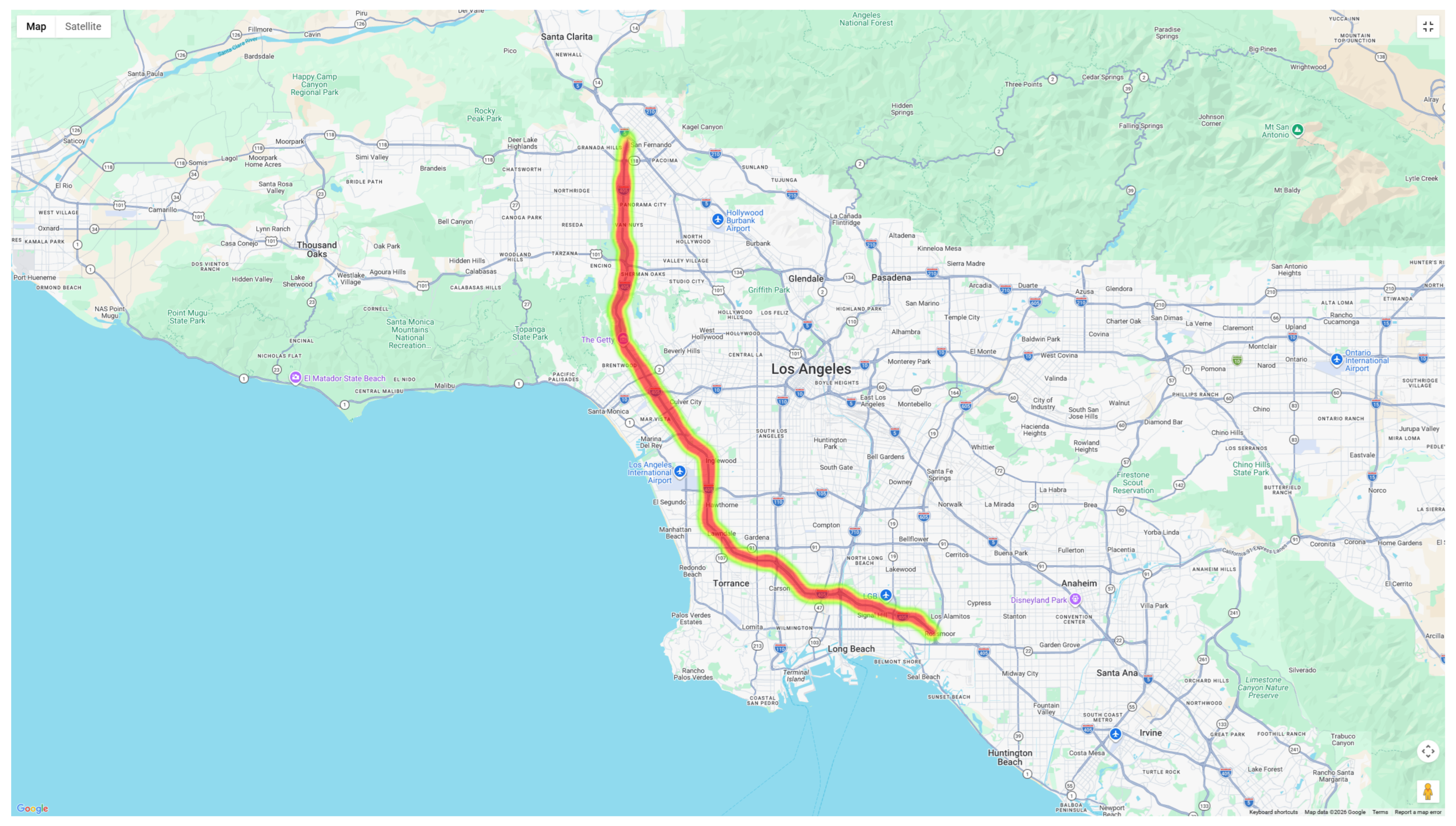
The traffic accident data used in this study were obtained from the Traffic Incident Management System (TIMS) released by the Federal Highway Administration (FHWA) [18]. The study focuses on a representative urban freeway segment, Interstate 405 (I-405), located in the Los Angeles metropolitan area of California, United States. The I-405 corridor was selected as a representative urban freeway due to its high traffic demand, complex interchange structure, diverse accident patterns, and long-term availability of high-quality accident records, which together provide a challenging and realistic testbed for accident time-series prediction.

Although the experiments in this study are conducted on a single freeway corridor, the proposed modeling framework is not tied to any specific roadway and is designed to capture general temporal characteristics of sparse and bursty accident time series, making it applicable to other urban freeway scenarios with similar data availability.

From a methodological perspective, the proposed approach focuses on learning general temporal patterns of sparse and bursty accident sequences, rather than corridor-specific spatial characteristics. To further examine the generalization capability of the model beyond a single freeway, extensive experiments were additionally conducted on two public benchmark time-series datasets (ETTh1 and Electricity), which exhibit diverse temporal dynamics and statistical properties. The consistent performance gains observed across these datasets indicate that the proposed framework is not limited to a specific corridor and can generalize to other traffic-related time series scenarios.

In this study, the prediction target is defined as the hourly accident count aggregated over the selected freeway corridor, resulting in a univariate time-series forecasting task.

The geographical location of the selected freeway segment is illustrated in Figure 4.

The original dataset contains detailed information for each traffic accident event, including occurrence time, geographic coordinates, roadway name, accident severity level, and casualty statistics. After data screening and preprocessing, accident records from January 2018 to December 2024 were retained, resulting in approximately 10,253 valid accident events. Each record corresponds to a single traffic accident occurrence.

After aggregating individual accident events into an hourly time series, the final dataset contains approximately 61,000 time steps spanning from January 2018 to December 2024. The resulting accident count series exhibits a highly imbalanced distribution.

Specifically, the majority of hourly intervals contain zero recorded accidents, while a smaller proportion of time steps correspond to one or two accidents. Only a limited number of periods exhibit multiple accidents within the same hour, representing high-risk traffic conditions. This pronounced sparsity and long-tailed distribution further highlight the challenges of traffic accident forecasting and motivate the use of risk-oriented evaluation metrics beyond conventional error-based measures. The distribution of hourly accident counts after aggregation is summarized in

Table 1. Distribution of hourly accident counts after aggregation.

Accident Count per Hour	Percentage (%)
0	81.0
1	13.2
2	3.8
≥3	2.0

.

This distribution further confirms the strong sparsity and long-tailed nature of the accident time series.

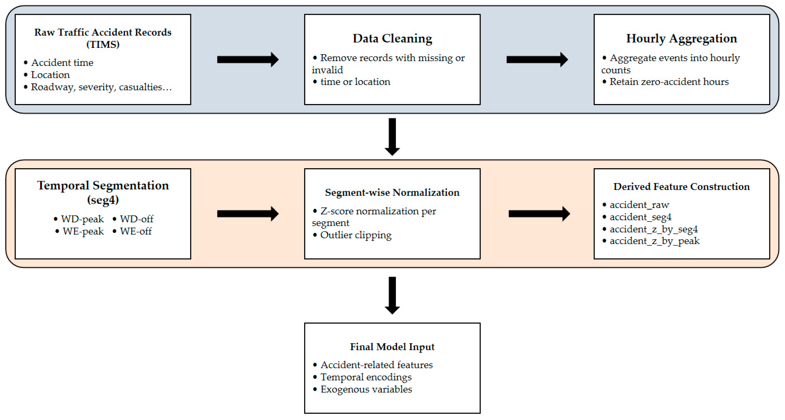
During preprocessing, records with missing or invalid key attributes (e.g., accident time or location) were removed. The remaining accident events were aggregated into an hourly time series with a continuous temporal index. Hours without recorded accidents were explicitly retained as zero-valued entries, ensuring temporal continuity without artificial interpolation.

Table 2. Sample records of raw traffic accident data.

COLLISION_DATE	COLLISION_TIME	PRIMARY_RD	SECONDARY_RD	COLLISION_SEVERITY	NUMBER_KILLED	NUMBER_INJURED	LATITUDE	LONGITUDE
1 January 2018	1832	I-405 N/B	WILSHIRE BLVD	2	0	2	34.0522	−118.4453
5 January 2018	0720	I-405 S/B	VENTURA FWY	3	0	1	34.1679	−118.4966
14 June 2021	0815	I-405 N/B	SUNSET BLVD	2	0	1	34.0983	−118.3637
22 October 2024	1748	I-405 S/B	CULVER BLVD	3	0	3	34.0211	−118.3965

provides representative accident records sampled from different years (2018, 2021, and 2024) to illustrate the structure and temporal coverage of the raw data.

A sample of the original accident records is presented in Table 2, which includes the collision date and time, primary and secondary road names, accident severity, number of injuries and fatalities, as well as latitude and longitude information.

To meet the input requirements of time series forecasting models, individual accident events on the I-405 freeway were aggregated into a univariate time series representing the number of accidents per hour. The resulting sequence exhibits pronounced temporal characteristics, including clear periodic patterns (e.g., weekday–weekend differences and peak–off-peak variations) as well as strong burstiness caused by holidays, extreme weather conditions, or abnormal traffic disturbances. In addition to the accident count series, multiple exogenous variables were constructed to enrich the model input and enhance interpretability.

Traffic accident distributions vary significantly across different time periods. Accident occurrences are frequent during peak hours, while late-night and early-morning periods on weekends tend to be sparse, leading to substantial differences in both mean and variance across time segments. Direct normalization of the entire sequence may suppress informative signals during sparse periods while allowing peak-hour patterns to dominate the learning process. To alleviate this issue, a segmented normalization strategy (denoted as seg4) was adopted.

Specifically, the time series was divided into four temporal categories: weekday peak hours (WD-peak), weekday off-peak hours (WD-off), weekend peak hours (WE-peak), and weekend off-peak hours (WE-off). Z-score normalization was applied independently within each segment, followed by value clipping to suppress extreme outliers [19]. This preprocessing strategy preserves overall temporal trends while improving the representation of sparse accident occurrences, thereby enhancing model robustness under complex temporal conditions.

Based on the segmented normalization strategy (seg4), several accident-related features were constructed. Specifically, the variable accident_seg4 represents the raw hourly accident count assigned to its corresponding temporal segment (WD-peak, WD-off, WE-peak, or WE-off). The feature accident_z_by_seg4 is obtained by applying Z-score normalization to the accident counts within each segment independently, using the segment-specific mean and standard deviation. This operation ensures that accident intensities are normalized relative to comparable temporal contexts rather than the entire time series.

In addition, accident_z_by_peak is derived by normalizing accident counts with respect to peak-hour statistics only, which emphasizes relative accident severity during high-demand traffic periods. All normalization parameters are computed exclusively from the training data to avoid information leakage.

Without this segmented normalization, the strong dominance of peak-hour accident patterns would bias the learning process, making it difficult for the model to effectively capture low-frequency accident signals during off-peak periods. Figure 5 illustrates the overall preprocessing pipeline used to transform raw traffic accident records into model-ready time series features.

The final feature set used for model training and evaluation is summarized in

Table 3. Feature structure after data preprocessing.

Category	Feature Name(s)	Type (Encoding)	Description
Temporal cycle	hour_sin, hour_cos	Continuous [−1,1]	Cyclic encoding of hour-of-day
Weekly cycle	dow_sin, dow_cos	Continuous [−1,1]	Cyclic encoding of day-of-week
Weather conditions	WEATHER_1, WEATHER_1_A, WEATHER_1_B, …	One-hot	Major weather categories (A/B/C/E/F/G)
Lighting conditions	LIGHTING_-, LIGHTING_A, …	One-hot	Lighting conditions (daylight, nighttime, street lighting, etc.)
Road surface	ROAD_SURFACE, ROAD_SURFACE_A, ROAD_SURFACE_B, …	One-hot	Road surface conditions (dry, wet, snow-covered, etc.)
Calendar indicators	is_weekend, is_peak, is_holiday	0/1	Weekend, peak-hour, and holiday indicators
Target and derived features	accident_raw, accident, seg4, accident_z_by_seg4, accident_z_by_seg4_clip3, accident_z_by_peak, …	Continuous/Categorical	Accident counts and segment-wise normalized features

, which includes temporal cyclic encodings, environmental conditions, road surface information, calendar indicators, and multiple accident-related derived features.

3.2. Experimental Setup and Evaluation Metrics

To evaluate the effectiveness of the proposed model for traffic accident prediction, a series of systematic experiments were conducted, including model training configuration, evaluation metrics, hyperparameter sensitivity analysis, and performance comparisons with multiple baseline methods. All experiments were implemented in a unified experimental environment to ensure fairness and reproducibility.

3.2.1. Experimental Configuration

All experiments were carried out on a local workstation running the Windows 11 operating system. The proposed model and baseline methods were implemented using Python 3.9 and the PyTorch 1.12 deep learning framework. The hardware platform consisted of an AMD Ryzen 7 9700X CPU and an NVIDIA GeForce RTX 5070 Ti GPU. Automatic Mixed Precision (AMP) was enabled during training to accelerate computation and reduce memory consumption.

The detailed experimental environment and configuration are summarized in

Table 4. Experimental environment and configuration.

Category	Specification
Operating system	Windows 11 (64-bit)
CPU	AMD Ryzen 7 9700X (8 cores, 16 threads)
GPU	NVIDIA GeForce RTX 5070 Ti
Memory	8 GB GPU memory, 32 GB system memory
Programming language	Python 3.9
Deep learning framework	PyTorch 1.12
Numerical precision	Automatic Mixed Precision (AMP)
Dataset split	Training:Validation:Testing = 6:2:2
Normalization	Z-score normalization

.

For all models, the same input window length, forecasting horizon, and dataset partitioning strategy were adopted to ensure a fair comparison. Model training was performed using the training set, hyperparameters were selected based on validation performance, and final results were reported on the test set.

3.2.2. Evaluation Metrics and Baseline Models

To comprehensively assess the prediction accuracy of the proposed model, two widely used regression metrics were adopted: Mean Squared Error (MSE) and Mean Absolute Error (MAE) [20]. MSE emphasizes large prediction errors by squaring deviations, while MAE measures the average absolute difference between predicted and ground-truth values, providing stable and interpretable error estimation.

The evaluation metrics are defined as follows:

$$MSE={\displaystyle \frac{1}{n}}{\displaystyle \sum _{i=1}^n{({\widehat{y}}_i-y_i)}^2},$$

(4)

$$MAE={\displaystyle \frac{1}{n}}{\displaystyle \sum _{i=1}^n|{\widehat{y}}_i-y_i|},$$

(5)

where n denotes the total number of samples, $y_i$ represents the ground-truth accident count at time step i, and ${\widehat{y}}_i$ is the corresponding predicted value.

Given the highly imbalanced nature of traffic accident data, where most time intervals contain zero or low accident counts and only a small number of periods exhibit accident surges, error-based metrics alone may not fully reflect a model’s practical effectiveness in safety-critical scenarios.

Therefore, in addition to MSE and MAE, we introduce Top-K Precision as a complementary evaluation metric to assess the model’s ability to correctly identify high-risk accident periods.

Specifically, let $T_K^{pred}$ denote the set of K time intervals with the highest predicted accident counts, and $T_K^{true}$ denote the set of K intervals with the highest observed accident counts. Top-K Precision is defined as:

$$\mathrm{Top}\text{-}\mathrm{K}\hspace{0.33em}\mathrm{Precision}={\displaystyle \frac{\left|T_K^{\mathrm{pred}}\cap T_K^{\mathrm{true}}\right|}{K}},$$

(6)

where $T_K^{pred}$ denotes the set of K time intervals ranked with the highest predicted accident counts, and $T_K^{true}$ denotes the set of K time intervals with the highest observed accident counts.

To validate the effectiveness of the proposed method, several representative time series forecasting models were selected as baseline methods. These baselines cover classical statistical approaches, recurrent neural networks, and state-of-the-art Transformer-based architectures. The selected baseline models are summarized as follows:

ARIMA [21]: A classical autoregressive integrated moving average model serving as a linear statistical baseline.

LSTM: A long short-term memory network designed to capture long-range temporal dependencies in sequential data.

Transformer: A self-attention-based sequence modeling architecture that captures global dependencies between arbitrary time steps, alleviating the gradient degradation problem of recurrent models.

Informer: A Transformer variant that introduces sparse attention mechanisms to improve efficiency for long-sequence forecasting tasks.

Autoformer: A decomposition-based Transformer model that incorporates trend–seasonality decomposition and autocorrelation mechanisms.

PatchTST: A state-of-the-art time series Transformer model based on patch segmentation and local representation learning.

BasisFormer (original): The baseline version of the BasisFormer model without patch encoding or structural enhancement.

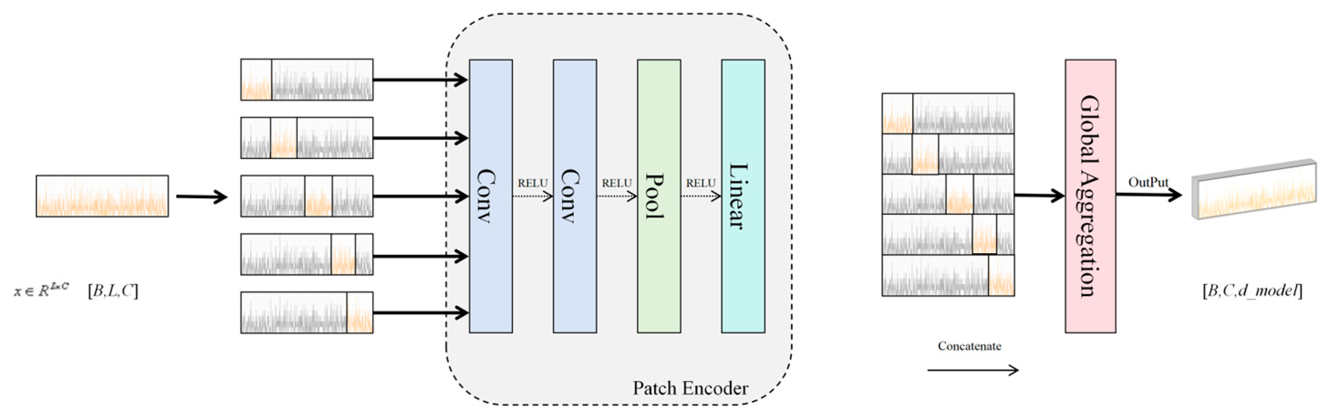
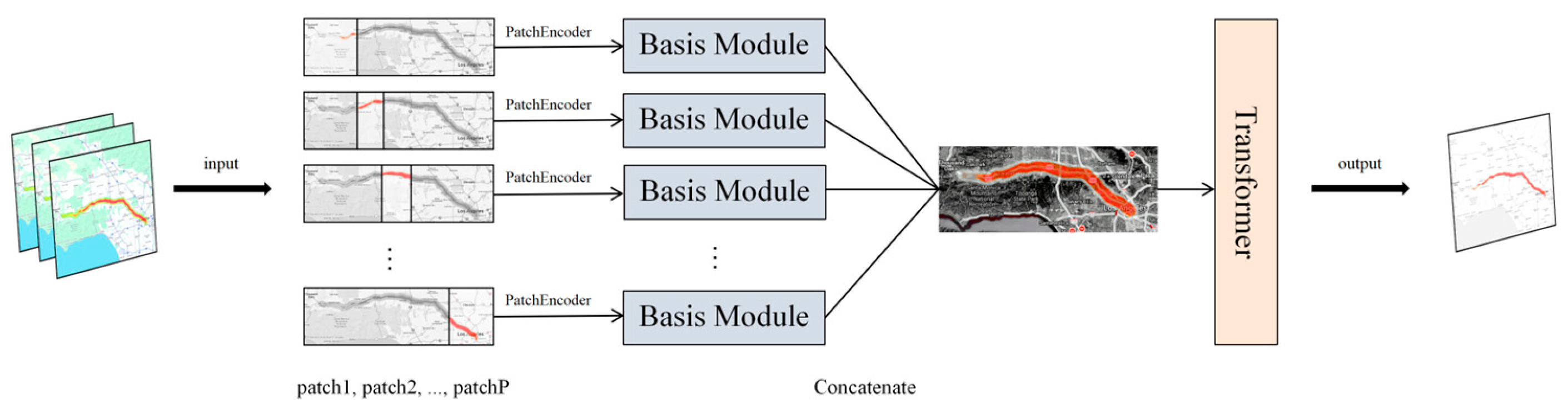
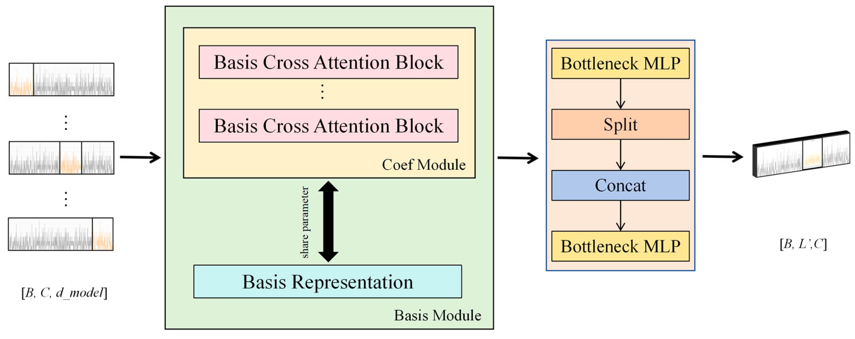
Ours: The proposed model, which integrates patch-aware local perception and multi-basis representation into the original BasisFormer framework.

All baseline models were trained and evaluated under the same experimental protocol, including identical input sequence lengths, forecasting horizons, and data splits. This ensures that the reported performance differences are attributable to model design rather than experimental bias.

3.3. Hyperparameter Sensitivity Analysis

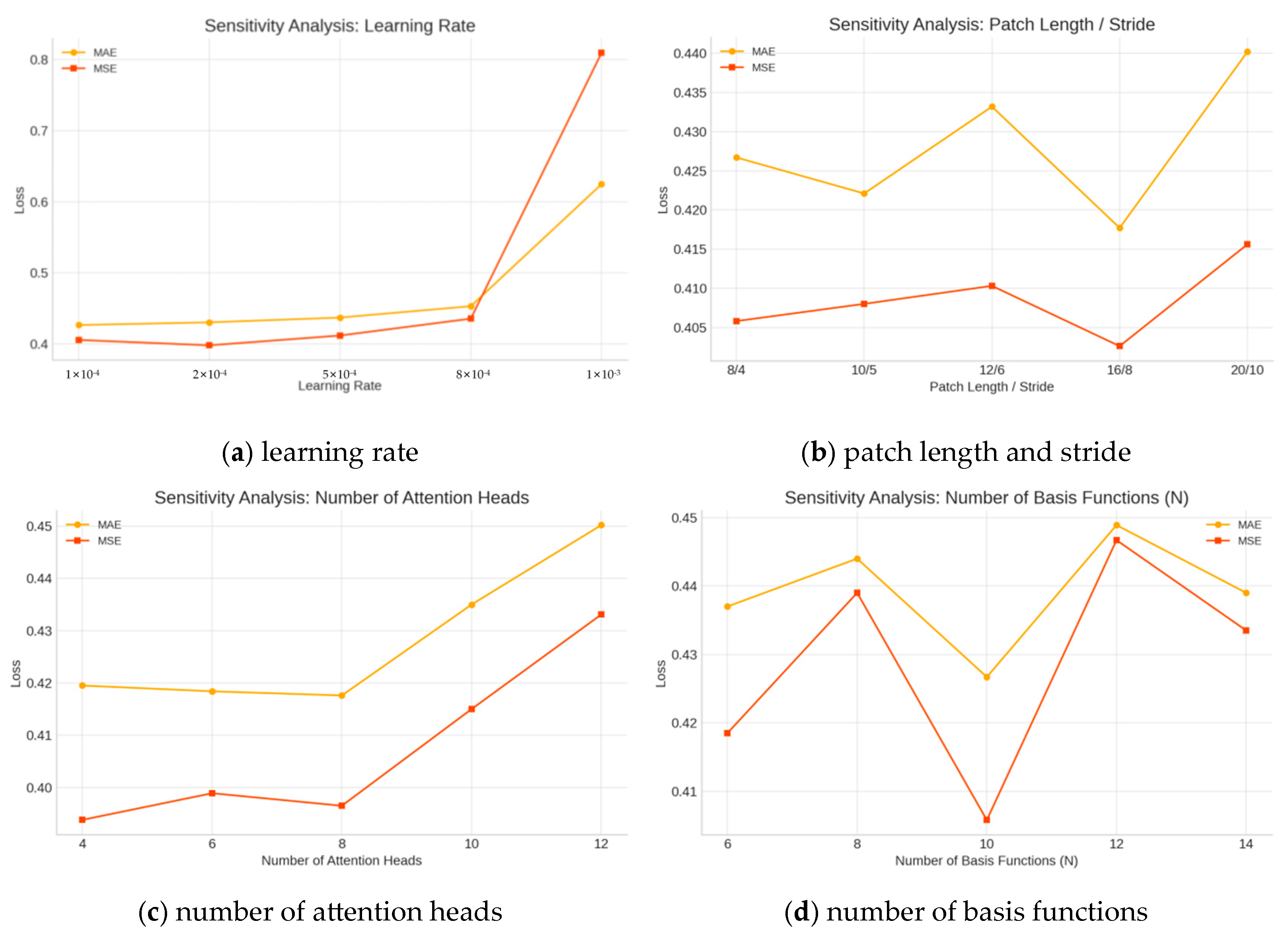
To evaluate the robustness of the proposed model under different hyperparameter settings and to analyze its performance stability, a comprehensive hyperparameter sensitivity analysis was conducted. Four key hyperparameters were investigated: the learning rate, patch segmentation strategy (i.e., patch length and stride), the number of attention heads, and the number of basis functions. For each hyperparameter, five representative values were tested while keeping all other settings unchanged. Model performance was evaluated on the validation set using Mean Squared Error (MSE) and Mean Absolute Error (MAE). The experimental results are illustrated in Figure 6.

As shown in Figure 6a, the model achieves relatively low error values when the learning rate is set to 1 × 10⁻⁴ or 2 × 10⁻⁴, indicating stable convergence behavior. When the learning rate increases to 1 × 10⁻³, both MSE and MAE rise significantly, suggesting that an excessively large learning rate may cause training instability or divergence. Therefore, smaller learning rates are more conducive to stable optimization and generalization performance.

Figure 6b presents the impact of different patch lengths and stride combinations on model performance. The results indicate that a patch configuration of 16/8 yields the lowest MSE, demonstrating that moderately increasing patch size can help capture local temporal structures more effectively. However, when the patch size becomes excessively large, performance degrades, which may be attributed to the over-smoothing of local patterns and the loss of fine-grained temporal information.

The influence of the number of attention heads is shown in Figure 6c. The model performs best when the number of heads is set to 4 or 6. In contrast, increasing the number of heads to 12 leads to a notable increase in prediction error. This phenomenon suggests that an excessive number of attention heads may cause information dispersion, thereby weakening the model’s ability to focus on salient temporal dependencies.

Figure 6d illustrates the effect of the number of basis functions on prediction accuracy. The optimal performance is achieved when the number of basis functions is set to N = 10. When N is either too small (e.g., N = 6) or too large (e.g., N = 14), the prediction error increases. This result indicates that an insufficient number of basis functions limits the model’s capacity to represent global temporal structures, whereas an overly large basis set may introduce redundancy and impair generalization.

Based on the sensitivity analysis, the primary hyperparameters of the proposed model were selected as summarized in

Table 5. Main hyperparameter settings of the proposed model.

Parameter	Value
patch_len	8
Patch stride	4
batch_size	32
d_model	128
heads	6
N	10
learning_rate	0.0005
train_epochs	100

.

3.4. Ablation Study

To further investigate the contribution of each key component in the proposed model, a systematic ablation study was conducted. Several core modules were progressively removed or simplified, and the resulting model variants were evaluated on multiple benchmark datasets. The ablation results are reported in

Table 6. Ablation study results on different datasets.

Model Variant	MSE (ETTh1)	MAE (ETTh1)	MSE (Traffic)	MAE (Traffic)
Full Model	0.3989	0.4184	0.5028	0.3355
w/o Patch (full-sequence input)	0.5875	0.5203	0.6653	0.4218
w/o Basis (number of bases = 1)	0.4208	0.429	0.6227	0.4062
w/o Smooth Loss	0.4172	0.4276	0.5205	0.343
w/o InfoNCE Loss	0.4106	0.4235	0.515	0.3402

.

As shown in Table 6, removing the patch-based encoding mechanism (denoted as w/o Patch) leads to the most significant performance degradation among all ablation settings. On the ETTh1 dataset, the Mean Squared Error (MSE) increases sharply from 0.3989 to 0.5875, while the Mean Absolute Error (MAE) rises from 0.4184 to 0.5203. This result indicates that for low-frequency time series with strong periodicity, such as electricity load data, the patch mechanism plays a crucial role in capturing local fluctuation patterns and enhancing short-term sensitivity.

In contrast, the Basis module exhibits a more pronounced impact on the Traffic dataset. When the number of basis functions is reduced to one (w/o Basis), the MSE and MAE increase to 0.6227 and 0.4062, respectively, which represents a substantially larger degradation compared with the ETTh1 dataset (0.3989→0.4208 in MSE). This observation suggests that for high-dimensional and multi-sensor traffic data with strong periodic structures, the Basis module serves as a core component for abstracting global trends and modeling cross-channel dependencies.

Further analysis of the auxiliary loss functions shows that removing the Smooth Loss or the InfoNCE Loss results in only minor performance degradation. These findings imply that the two auxiliary objectives mainly contribute to training stability and feature distribution regularization, while their direct impact on final prediction accuracy is relatively limited.

Overall, the ablation results demonstrate a complementary relationship between the Patch and Basis mechanisms. The Patch module is particularly effective in modeling low-frequency time series with pronounced local variations, whereas the Basis module provides stronger global modeling capability for high-frequency, high-dimensional datasets. By integrating both components, the proposed model achieves robust performance across diverse time series forecasting scenarios and maintains strong generalization ability.

3.5. Baseline Comparison Under Multiple Evaluation Metrics

3.5.1. Evaluation Under Standard Error Metrics

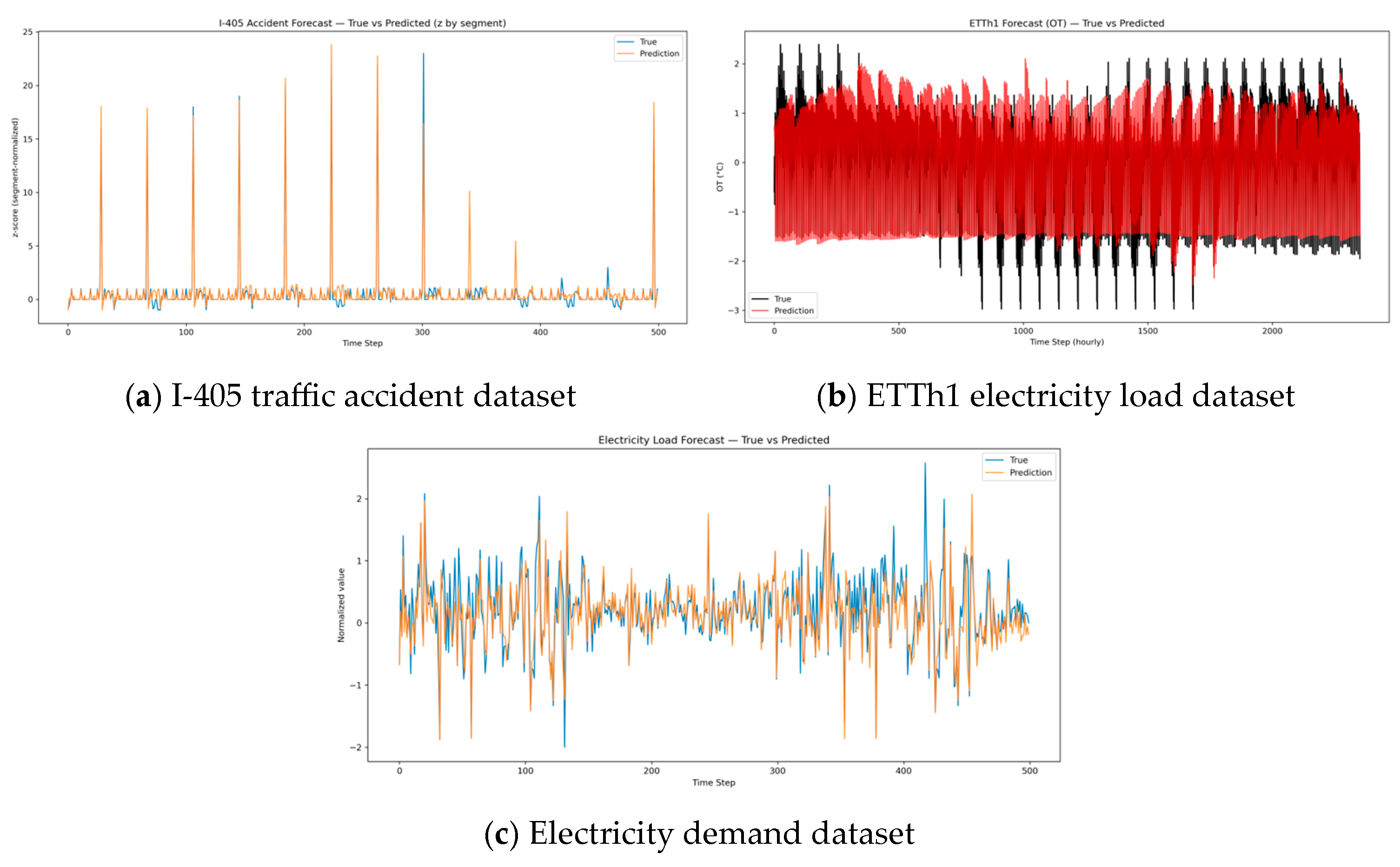
To further evaluate the effectiveness and generalization capability of the proposed model across different time series forecasting scenarios, visualized prediction results and quantitative comparisons were conducted on the I-405 traffic accident dataset as well as two public benchmark datasets, namely ETTh1 and Electricity. The prediction results are illustrated in Figure 7a–c.

As shown in Figure 7a, the traffic accident time series on the I-405 freeway exhibits high sparsity and significant amplitude variations. Despite these challenges, the proposed model accurately captures sparse peak patterns corresponding to accident surges. By employing patch-wise independent basis representations, the model effectively expresses multi-scale temporal patterns within segmented time windows while preserving global temporal dependencies. As a result, the model achieves a balanced representation of local abrupt changes and long-term trends, which is particularly suitable for accident prediction tasks characterized by burstiness and sparsity.

In the ETTh1 electricity load forecasting task (Figure 7b), the data exhibit strong periodicity and relatively stable temporal dynamics. The proposed model successfully captures the dominant periodic trends; however, slight phase shifts can be observed in some high-frequency fluctuation regions. This phenomenon suggests that under strongly periodic signals, the global basis representation plays a dominant role, while local patch information still has potential for further refinement in modeling fine-scale variations.

As illustrated in Figure 7c, the Electricity demand dataset demonstrates concurrent fluctuations across multiple users and regions. The proposed model is able to stably track short-term demand variations, with predicted curves closely aligning with ground-truth values in most time intervals. This result indicates that the combined patch-aware and basis-based architecture exhibits strong generalization capability in scenarios involving multi-variable and multi-region temporal interactions.

The quantitative performance comparison of all baseline models is summarized in

Table 7. Performance comparison of different models on multiple datasets.

Model	MSE (I-405)	MAE (I-405)	MSE (ETTh1)	MAE (ETTh1)	MSE (Electricity)	MAE (Electricity)
ARIMA	0.7812	0.5201	0.6589	0.5974	0.3276	0.3621
LSTM	0.6152	0.3929	0.5167	0.5289	0.2424	0.3031
Informer	0.5480	0.3573	0.4336	0.4450	0.1955	0.2735
Transformer	0.5750	0.3685	0.4681	0.4712	0.2134	0.2864
Autoformer	0.5366	0.3417	0.4175	0.4336	0.1887	0.2682
PatchTST	0.5127	0.3126	0.3134	0.3585	0.1573	0.2374
Basisformer	0.5956	0.3808	0.5875	0.5203	0.1692	0.2669
Ours	0.4630	0.2733	0.3989	0.4184	0.1655	0.2654

.

As reported in Table 7, the proposed model (Ours) achieves the best performance on the I-405 traffic accident dataset, with an MSE/MAE of 0.4630/0.2733. Compared with PatchTST, the proposed method achieves improvements of approximately 9.7% in MSE and 12.6% in MAE, and significantly outperforms BasisFormer as well as other state-of-the-art Transformer-based models such as Informer and Autoformer. These results demonstrate that the proposed model effectively captures the coexistence of abrupt events and periodic patterns in traffic accident data. The patch mechanism enhances responsiveness during accident peaks, while the basis representation improves stability during low-activity periods, leading to superior overall performance.

In contrast, classical statistical methods (e.g., ARIMA) and recurrent neural networks (e.g., LSTM) consistently underperform across all datasets. In particular, on the I-405 dataset, the MSE of ARIMA exceeds that of the proposed model by more than 60%, highlighting the limitations of shallow statistical models and simple sequential memory mechanisms when applied to highly non-stationary and sparse accident data.

On strongly periodic public datasets, differentiated performance characteristics are observed. For the ETTh1 dataset, which is dominated by energy consumption time series with weak burstiness, PatchTST achieves the best results (MSE/MAE = 0.3134/0.3585). Although the proposed model does not surpass PatchTST in this scenario, it outperforms Autoformer and Informer, indicating that the introduction of basis representations remains beneficial for capturing periodic trends. On the Electricity dataset, the proposed model achieves an MSE/MAE of 0.1655/0.2654, outperforming BasisFormer and approaching the performance of PatchTST. This suggests that the integration of patch-aware modeling and basis representations provides a balanced solution for datasets with concurrent local disturbances and global temporal patterns.

3.5.2. Evaluation Under Risk-Oriented Metrics

While standard error metrics such as MSE and MAE provide an overall assessment of average prediction accuracy, traffic accident forecasting is inherently risk-oriented, where the accurate identification of extreme accident periods is of greater practical importance. To further evaluate the proposed model under high-risk scenarios, two additional metrics are introduced: the 95th Percentile Mean Absolute Error (P95-MAE) and the Top-K Recall.

The P95-MAE measures the tail behavior of the error distribution and specifically reflects prediction stability during extreme periods characterized by high accident intensity and large fluctuations. In contrast, Top-K Recall evaluates the model’s ability to correctly identify high-risk time windows by comparing the overlap between the top-K time steps ranked by predicted accident intensity and those ranked by ground-truth values. These two metrics jointly assess the model’s performance from the perspectives of extreme error control and risk period identification, which are more aligned with the requirements of traffic safety analysis and early warning applications.

The P95-MAE is defined as:

$$\mathrm{P}95\text{-}\mathrm{MAE}={Percentile}_{95}(\left|y_t-{\widehat{y}}_t\right|),$$

(7)

where $y_t$ and ${\widehat{y}}_t$ denote the ground-truth and predicted accident values at time step t, respectively.

The Top-K Recall is defined as:

$$\mathrm{Top}\text{-}\mathrm{K} \mathrm{Recall}=\left|{\displaystyle \frac{\mathrm{\Omega }K\cap \widehat{\mathrm{\Omega }}K}{\mathrm{\Omega }K}}\right|,$$

(8)

where Ω_K represents the set of time steps corresponding to the top-K highest accident intensities in the ground truth, and ${\widehat{\Omega }}_k$ denotes the set of time steps ranked within the top-K according to model predictions.

The comparative results of all baseline models on the I-405 traffic accident dataset under these risk-oriented metrics are summarized in

Table 8. Performance comparison under risk-oriented evaluation metrics on the I-405 dataset.

Model	P95-MAE (I-405)	Top-K Recall (I-405, K = 10)
ARIMA	1.45	0.32
LSTM	1.18	0.46
Informer	1.07	0.53
Transformer	1.12	0.50
Autoformer	1.02	0.57
PatchTST	0.94	0.63
Basisformer	1.09	0.55
Ours	0.82	0.71

.

As shown in Table 8, traditional statistical models such as ARIMA and recurrent neural networks such as LSTM perform poorly in extreme accident scenarios, exhibiting both higher P95-MAE values and lower Top-K Recall scores. This indicates that shallow statistical assumptions and simple sequential memory mechanisms are insufficient for modeling highly sparse and bursty accident patterns.

Transformer-based models, including Informer and Autoformer, achieve moderate improvements in both metrics, with P95-MAE reduced to 1.07 and 1.02 and Top-K Recall increased to 0.53 and 0.57, respectively. However, their performance remains unstable in peak accident periods, suggesting limited sensitivity to abrupt risk escalation.

PatchTST demonstrates a stronger ability to capture short-term accident surges, achieving a Top-K Recall of 0.63 due to its patch-wise local modeling strategy. BasisFormer, on the other hand, benefits from interpretable global basis representations and achieves a Top-K Recall of 0.55, highlighting its strength in modeling structured temporal patterns.

The proposed model consistently outperforms all baselines across both metrics, achieving the lowest P95-MAE of 0.82 and the highest Top-K Recall of 0.71. Compared with PatchTST, the P95-MAE is reduced by approximately 12.8%, while the Top-K Recall is improved by approximately 29.1% compared with BasisFormer. These results demonstrate that the integration of patch-aware local perception and global basis representations significantly enhances the model’s sensitivity to high-risk accident periods without sacrificing long-term trend modeling capability.

Overall, the risk-oriented evaluation confirms that the proposed model not only achieves superior average prediction accuracy but also exhibits strong robustness and reliability in extreme accident scenarios. This dual advantage is particularly critical for traffic accident forecasting applications, where timely identification of high-risk periods is essential for proactive traffic safety management and early warning systems.

In addition to Top-K Recall, we further report Top-K Precision to evaluate the accuracy of high-risk period identification from a complementary perspective.

As shown in

Table 9. Top-K Precision comparison on the I-405 accident dataset.

Model	Top-5	Top-10	Top-20
ARIMA	0.4	0.33	0.25
LSTM	0.48	0.4	0.32
Informer	0.55	0.46	0.38
Transformer	0.52	0.44	0.36
Autoformer	0.57	0.48	0.39
PatchTST	0.62	0.54	0.45
BasisFormer	0.58	0.5	0.41
Ours	0.7	0.62	0.53

, the proposed model consistently achieves the highest Top-K Precision across different K values, indicating its superior capability in accurately identifying high-risk accident periods compared with baseline methods.

3.6. Interpretability Analysis

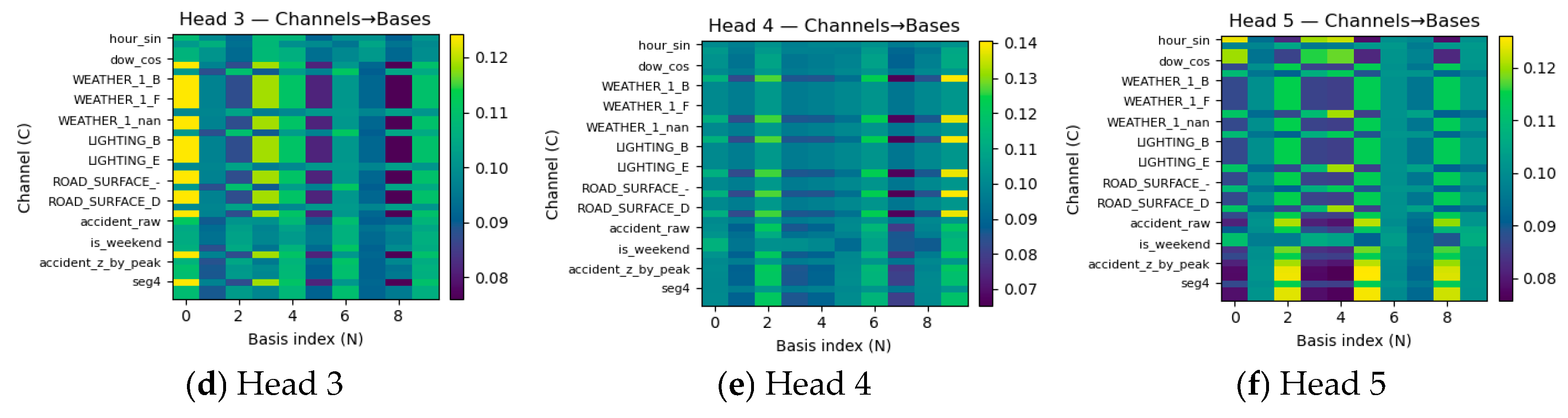
To further understand the decision-making mechanism of the proposed model in traffic accident forecasting, an interpretability analysis was conducted by visualizing the learned attention weights within the basis-aware attention module. The visualization aims to reveal how different input feature channels contribute to the learned basis representations under a multi-head attention mechanism.

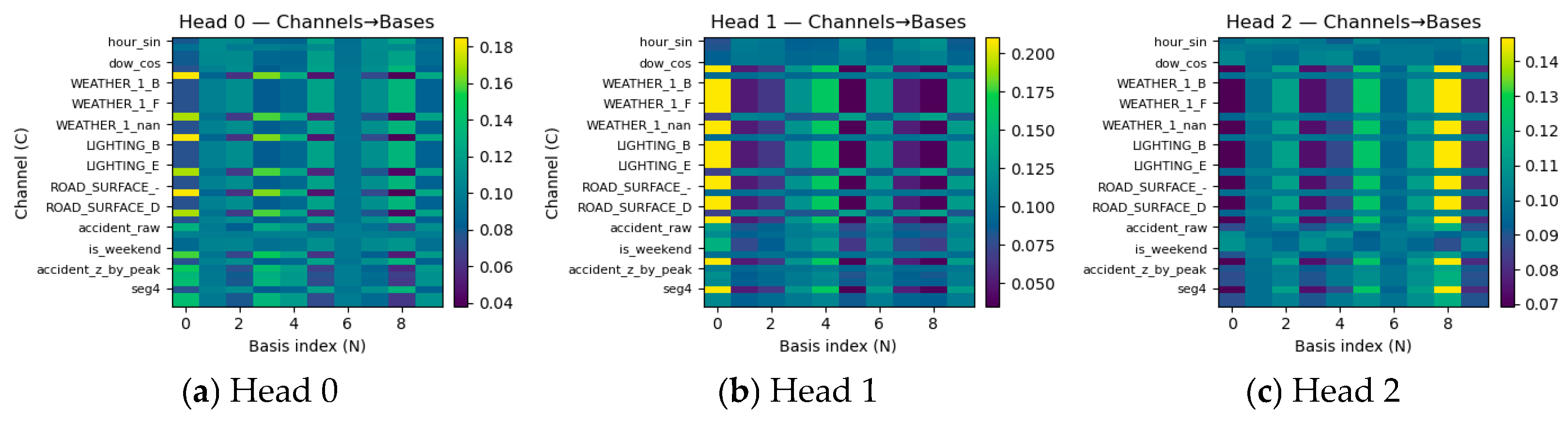
Figure 8 presents the attention heatmaps learned by the proposed model on the I-405 traffic accident dataset. The horizontal axis represents the basis index (N = 10), while the vertical axis corresponds to different input feature channels, including temporal encodings, environmental factors, and historical accident-related variables. Color intensity indicates the magnitude of attention weights, reflecting the relative importance of each feature channel to a specific basis representation. Each subfigure corresponds to one attention head (Head 0–Head 5), illustrating the diversity of feature–basis associations learned across multiple subspaces.

As shown in Figure 8, temporal features such as hour_sin, dow_cos, and is_weekend consistently receive high attention weights across multiple heads, indicating that the model strongly relies on daily and weekly periodic patterns as well as weekend effects when modeling accident occurrence. This observation aligns well with the inherent temporal regularities of traffic accidents, which are closely associated with peak-hour traffic demand and weekday–weekend travel behavior.

Historical accident-related features, including accident_raw and accident_z_by_peak, also exhibit prominent attention weights in several heads. This suggests that recent accident intensity and peak-period normalized signals play a critical role in shaping the basis representations used for future prediction. The result further validates the effectiveness of the segmented normalization strategy adopted in data preprocessing, as these features become salient components in the learned basis combinations.

In contrast, external environmental variables such as weather conditions (WEATHER_1_B, WEATHER_1_F), lighting conditions (LIGHTING_B, LIGHTING_E), and road surface states (ROAD_SURFACE) demonstrate more heterogeneous attention patterns across different heads. This indicates that the multi-head attention mechanism captures complementary contextual information in different subspaces, allowing the model to selectively emphasize environmental factors under varying temporal and traffic conditions rather than assigning them uniform importance.

Notably, distinct attention heads exhibit markedly different basis allocation patterns even for the same feature channel. For example, Head 0 and Head 2 attend to different basis indices for hour_sin, implying that the model learns multiple latent temporal abstractions for the same input signal. This diversity confirms that the multi-head attention mechanism is not redundant but instead enables the model to disentangle complex feature–basis relationships and capture heterogeneous accident patterns at multiple temporal scales.

Overall, the interpretability analysis demonstrates that the proposed model effectively integrates temporal regularities, historical accident dynamics, and contextual environmental factors through basis-aware attention. By learning structured and interpretable feature–basis associations, the model provides not only accurate predictions but also meaningful insights into the underlying mechanisms driving traffic accident risks, thereby enhancing its applicability in practical traffic safety analysis and decision support systems.

4. Conclusions

In this study, a traffic accident forecasting model integrating patch-aware local perception and global basis representations was proposed to address the challenges of sparsity, burstiness, and strong periodicity commonly observed in accident time series. By combining localized patch segmentation with interpretable basis modeling, the proposed framework aims to balance short-term abrupt pattern capture and long-term structural trend alignment within a unified architecture.

Experimental results on the I-405 traffic accident dataset demonstrate that the proposed model consistently outperforms classical statistical methods and state-of-the-art deep learning baselines under standard error metrics. Compared with representative Transformer-based models, the proposed approach achieves lower MSE and MAE values, indicating superior overall prediction accuracy for highly non-stationary and sparse accident data. Additional evaluations on public benchmark datasets further verify the model’s generalization capability across different types of time series forecasting tasks.

Beyond average accuracy, the proposed model exhibits clear advantages in high-risk scenario identification. Under risk-oriented evaluation metrics, including P95-MAE and Top-K Recall, the model achieves more stable predictions during extreme accident periods and more accurately identifies high-risk time windows. These results highlight the effectiveness of integrating patch-level sensitivity with global basis alignment for traffic safety–oriented forecasting tasks, where reliable extreme-event prediction is of critical importance.

Furthermore, interpretability analysis based on attention weight visualization reveals that the model learns meaningful feature–basis associations across multiple attention heads. Temporal periodic features, historical accident signals, and contextual environmental factors are selectively emphasized under different latent subspaces, providing insights into the mechanisms driving accident risk formation. This interpretability enhances the transparency and practical applicability of the proposed framework in real-world traffic safety analysis and decision-making support.

Despite the encouraging results, this study still has limitations. The current model is evaluated on a single freeway corridor for accident prediction, and future work will consider extending the framework to larger-scale road networks and multi-source spatiotemporal data. In addition, incorporating real-time traffic flow information and exploring adaptive basis learning strategies may further improve predictive robustness under rapidly changing traffic conditions.

Overall, the proposed patch-aware and basis-integrated forecasting framework provides an effective and interpretable solution for traffic accident prediction. The results suggest that combining local perception mechanisms with structured global representations is a promising direction for improving both prediction accuracy and risk-awareness in intelligent transportation safety systems.