Application of Queuing Theory in the Reliability and Risk Assessment of the Water Supply System: Case Study of the Jabal Hasouna Well-Field

Abstract

To address water shortages, Libya has undertaken one of the most significant global civil infrastructure projects, the Great Man-Made River Project, aimed at transporting groundwater from southern well-fields to densely populated northern cities. The second phase of the project consisted of installing the water supply system, which comprises 479 well pumps, united to deliver around 2 million cubic meters of water to the north. Historical performance data for the water supply system were analyzed, and a model for the system’s reliability calculation was developed: a finite-source, multi-server queuing system with spares (M/M/c//N/Y). The model enabled the analytical calculation of the system’s reliability in different configurations. Each configuration was assessed using a unique risk score, defined as the product of reliability-based parameters and the consequences associated with water-shortage events resulting from system failures. The analysis identified two alternative configurations that satisfy all predefined performance and risk criteria. Both configurations require fewer resources than the original system design, with up to seven fewer spare pumps, allowing for decision-makers to select the most appropriate option based on additional operational and contextual considerations.

1. Introduction

Water scarcity poses a major threat to development and stability in arid and semi-arid regions, making effective management of water resources essential. In such regions, water supply depends heavily on groundwater, long-distance transfer, and highly reliable abstraction and distribution systems. In Libya, where renewable surface water is extremely limited and reliance on deep fossil aquifers is high, significant investments have been made in large-scale groundwater infrastructure. The Great Man-Made River Project (GMRP) exemplifies one of the world’s largest civil engineering and water conveyance initiatives, transporting groundwater from southern desert well-fields to coastal settlements and agricultural centers. Groundwater remains one of the most reliable sources of potable and industrial water, supplying nearly half of global drinking water demand. Well-fields, consisting of multiple production wells, enhance resilience over single sources; however, they remain vulnerable to mechanical or electrical failures, aquifer yield reductions, water quality deterioration, and external shocks such as power outages [1,2].

Libya relies mainly on groundwater resources located deep beneath its desert, making it one of the most water-scarce countries in the world. In response to this challenge, the Libyan government launched a major infrastructure project called the Great Man-Made River Project (GMRP) in the 1980s. The project was designed to transport groundwater over long distances to northern coastal towns and agricultural areas. The United Nations Environmental Program (UNEP) identifies the GMRP as one of the largest civil engineering projects worldwide [3]. 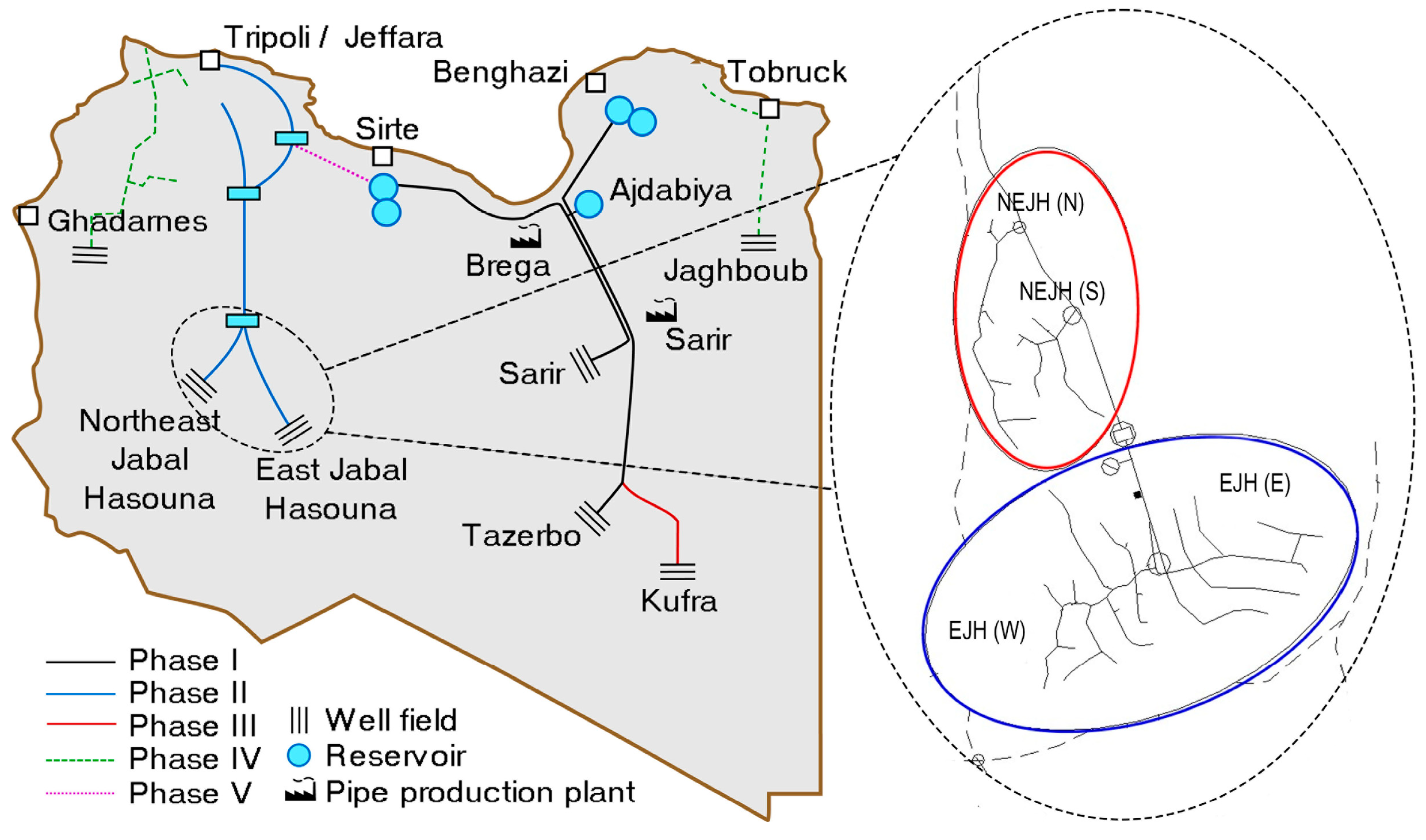Research shows that the water supplied by the GMRP is five times more cost-effective than any other water delivery alternative [4]. The project consists of five distinct phases (Figure 1) [5,6]:

• Sarir-Sirte/Tazerbo—Benghazi System;
• Jabal Hasouna—Jeffara Water System;
• Ghadames-Zwara—Zawia System;
• Kufra—Tazerbo System;
• Ajdabiya—Tobruk System.

Figure 1. Layout of the GMRP and the Jabal Hasouna well-field scheme (adapted from [6,7]).

Figure 1. Layout of the GMRP and the Jabal Hasouna well-field scheme (adapted from [6,7]).

The project’s ultimate goal, once completed, is to deliver about 6 million cubic meters (m³) of water every day from the desert, where southern sources are, to nearby areas and northern regions, where the need for clean and safe water is becoming increasingly urgent.

The Jabal Hasouna well-field (Figure 1) [7], which is part of GMRP Phase II (Western Jamahiriya System), plays a vital role in transporting groundwater from wells located east and northeast of Jabal Hasouna (EJH (E&W) and NEJH (N&S)) to urban and agricultural areas in the western region. The goal of this project phase is to supply 2.003 million cubic meters of water daily (m³/day), with potential expansion capacity up to 2.5 million cubic meters in a later phase. This is achieved by utilizing four well-fields collectively called the Jabal Hasouna well-field, which includes a total of 479 production wells. All well pumps are submersible, with nominal outputs ranging from 25 to 60 L per second [5,8].

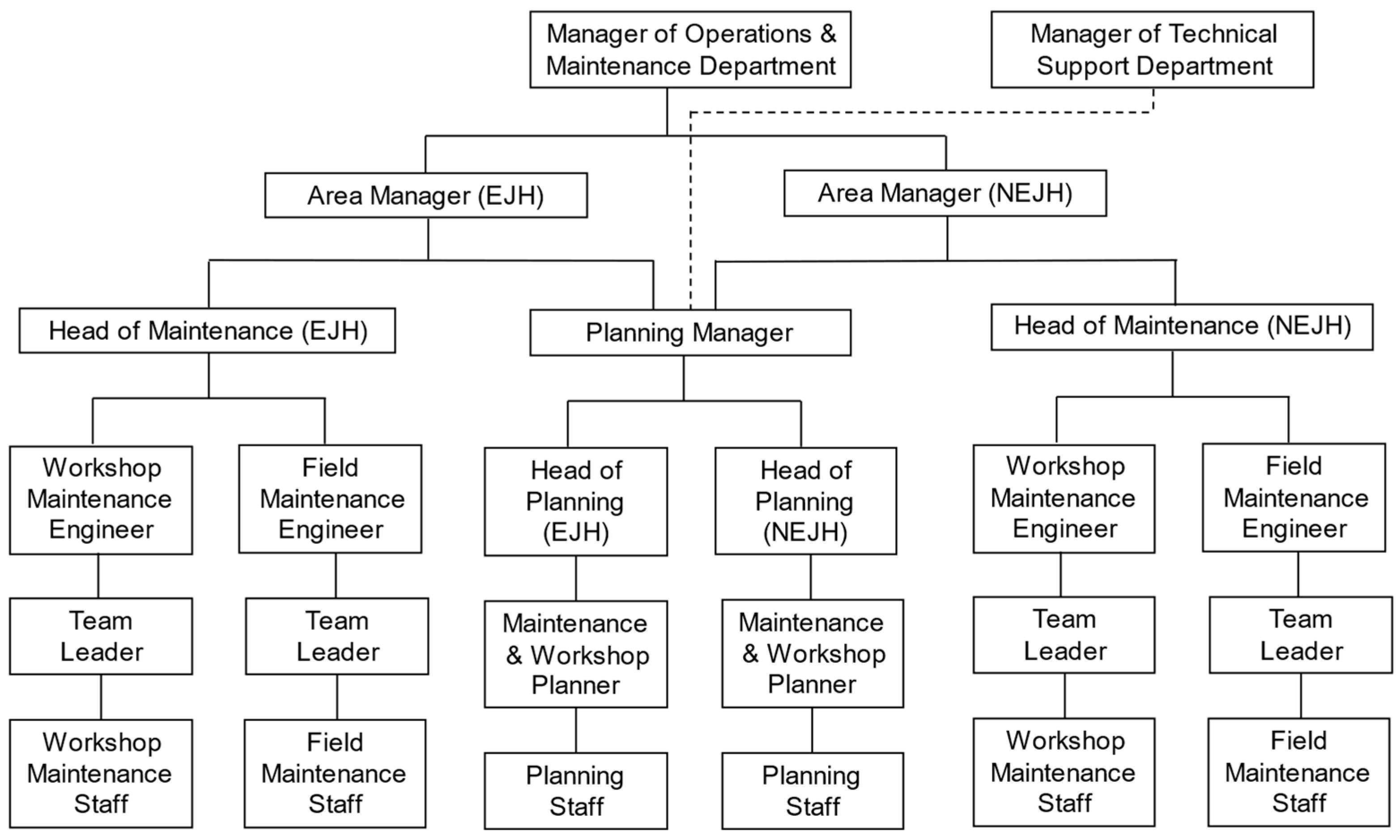
Due to the extensive size of the Jabal Hasouna area, the organizational structure of the maintenance subsystem is decentralized, i.e., divided into two primary area groups (EJH and NEJH), each responsible for a designated region to enhance the coverage of monitoring and maintenance activities. The organizational structure scheme and additional system details are shown in Appendix A.

This study investigates the reliability (According to Goulter [9], the reliability of a water distribution (supply) system is defined as its capacity to satisfy the demands placed upon it, specifically in terms of the required flow volumes and rates, and the pressure ranges at which these flows must be delivered. Cullinane et al. [10] further interpret this as the system’s ability to continue providing service with an acceptable level of interruption, even under abnormal conditions) and risk of the Jabal Hasouna water supply system using a queuing theory-based model. The research addresses the following questions: (1) How reliable is the system under current operational conditions? (2) How do maintenance resources, such as the number of maintenance teams and spare pumps, affect system performance and downtime? (3) How can queuing theory be applied to quantify the probability of system failure and associated risks? (4) How can these insights support operational and tactical decision-making for maintenance planning?

In line with these research questions, this study makes three main contributions. First, it provides an analytical determination of the water supply system’s reliability at the Jabal Hasouna well-field using a queuing theory-based approach. Second, it proposes a reliability-based risk assessment framework that quantifies the probability of system failures and evaluates the associated operational risks. Third, it develops a decision-support methodology within the queuing theory framework to identify the optimal system configuration, specifically determining the minimum number of spare pumps and field repair teams required to maintain an acceptable level of risk. Together, these contributions establish a clear link between analytical modeling, risk assessment, and practical decision-making, enhancing both the theoretical and practical value of the study.

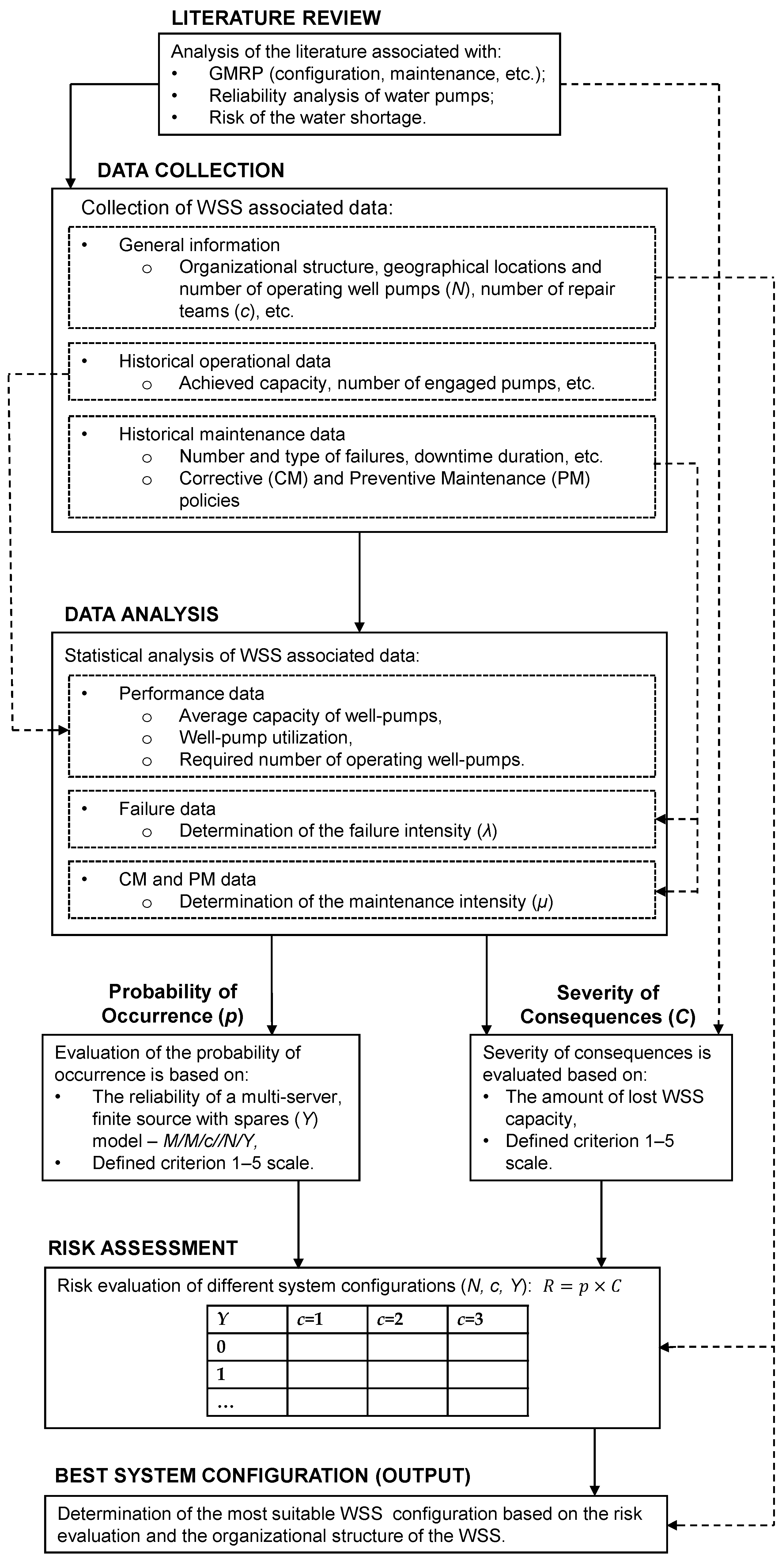
The paper is organized into eight sections. Section 1 provides basic information on the Jabal Hasouna well-field, including its spatial layout, the Phase II production target, along with a review of the relevant literature on maintenance, reliability, and WSS risk assessment. Section 2 outlines the methodology for WSS risk assessment based on system reliability, including how to determine the WSS configuration that ensures a low-risk level. Section 3 describes the database structure used for statistical analysis of WSS maintenance data. Section 4 presents the statistical analysis of input data conducted to determine the required number of operating pumps, pump reliability, failure rates, and overall maintenance intensity. Section 5 identifies the WSS operating parameters using a finite-source, multi-server queuing theory model with spares. Section 6 introduces the WSS risk assessment model and evaluates risk for different WSS configurations. Section 7 discusses the results, summarizes the main findings, and determines the WSS configuration required to meet the Phase II objectives with an acceptably low risk. Finally, Section 8 presents the paper’s conclusions.

Literature Review

The reliability of a water distribution system refers to its capacity to deliver an adequate level of service to customers during both normal and abnormal operating conditions within a specified time frame. This definition has guided the scientific community over the past thirty years. The reliability of the WSS can be categorized into three main types: (1) mechanical, which includes failures of components such as pipelines, valves, and pumps; (2) hydraulic, which relates to fluctuations in boundary variables, including user demands; and (3) quality reliability, which addresses issues related to water quality [11].

Reliability analysis of water distribution systems has long been a focus in the engineering literature. One of the most fundamental research approaches to this problem was conducted by Mays [12] at the end of the last century. The study presented the framework for an approach, which was novel at the time, related to the reliability of water supply networks. It included evaluations of pumping facility reliability and optimization models for water distribution network reliability. Reliability was assessed using Monte Carlo simulation for both the model and the system. Pumping facility reliability was evaluated through frequency and duration analyses addressing mechanical and hydraulic failures. The study further presented a reliability-based optimization framework for water supply networks, integrating nonlinear programming, simulation and reliability modeling.

Furthermore, in order to assess advancements and discoveries in the field of reliability in water distribution systems at the start of the 21st century, Sirsant et al. [13] performed a bibliometric analysis. This review examined 347 relevant publications published between 2000 and 2022. The study identified three main categories: (1) Reliability, which includes articles focused on the reliability-based design of Water Distribution Networks and explores hydraulic and mechanical failures, as well as uncertainties; (2) Water Distribution Networks, which centers on the design and modeling of WDNs; and (3) Optimization, which covers various techniques aimed at improving the designs of WDNs.

Based on the analyzed research, the work that attracted the most attention was conducted by Ostfeld [14]. The paper compared two reliability assessment approaches for water distribution systems: a simplified model integrating topological and hydraulic reliability for lumped supply–demand networks, and a probabilistic Monte Carlo-based model applicable to general networks using EPANET. Ostfeld further classified reliability assessment methods into connectivity (topological), hydraulic, and entropy-based categories. Similarly, Naguib et al. [15] developed a methodology consisting of seven steps to evaluate the reliability of water distribution networks and identify the best upgrade scenarios for improvement. These steps, in order, were building a hydraulic model, calculating component availability, assessing hydraulic reliability, assessing mechanical reliability, evaluating overall network reliability, defining upgrade options, and conducting optimization analyses. Alshaari and Nor [16] studied water pump reliability by analyzing metrics such as mean time between failures (MTBF), mean time to repair (MTTR), and availability. They performed a comparative analysis of different pump brands using a Mean Cumulative Function (MCF) plot and proposed improvement strategies based on the Failure Modes, Effects, and Criticality Analysis (FMECA) technique.

Conversely, the unreliability of water distribution systems is directly linked to their inherent risk. In other words, every delay or failure of a machine has its probability and consequences, which impact the rest of the system if such an event occurs. These two components are fundamental parts of risk by definition [17]. Therefore, it is recommended for the system to shift from a reliability maximization strategy to a risk-based reliability evaluation method. Determining the absolute reliability of systems and complex processes is very challenging, especially with scarce failure data. As a result, reliability studies have mainly relied on probability theory, where failure time is predicted once the failure distribution type is identified. Khalaj et al. [18] introduced the concept of risk-based reliability evaluation as an innovative approach for decision-making in risk assessment, especially focusing on epistemic uncertainty caused by limited evidence. This study used the Dempster–Shafer Theory to clarify different types of uncertainty and their effects, while also assessing the risk of a production system through a risk matrix, ultimately determining its relevance for production companies.

Christodoulou et al. [19] proposed a proactive, risk-based integrity monitoring framework for sustainable management of urban water distribution networks, combining artificial neural networks with parametric and nonparametric survival analysis to identify risk factors and estimate time-to-failure. Building on this risk-oriented perspective, Raspati et al. [20] developed a risk-based pipe rehabilitation strategy that integrates data-driven failure probability estimation using Random Forests with hydraulic reliability assessment, synthesizing probabilistic and impact analyses through a risk-matrix representation to support utility decision-making.

Despite the extensive literature aimed at improving the management of complex water supply systems, there remains a notable gap in research proposing practical approaches that combine reliability and risk-assessment methodologies to optimize these systems. The scarcity of the relevant literature increases when the topic is bounded explicitly by the needs of the GMRP project, as previous research has primarily focused on water management, water quality; water extraction; aquifer behavior, monitoring, and control; and water costs, often examining these topics separately. For instance, Elhassadi [21] used two models to predict water resource costs. The first model evaluated the costs related to operation and maintenance, while the second analyzed the electricity costs involved in water production. Gijsbers et al. [22] enhanced the mathematical optimization models for each setup of the GMRP desalination systems. Therefore, the gap in reliability-oriented research is significantly relevant when focusing on Libya and the Jabal Hasouna well-field. This issue is particularly concerning due to frequent failures of critical equipment, including pumps, wellhead components, and pumping stations, which directly affect the urban water supply.

When addressing the challenge of providing a reliable water supply system, the literature consistently emphasizes the importance of incorporating reliability analysis and risk assessment from the earliest stages of the design process for complex systems. Unlike simple capacity analyses, reliability studies include availability metrics, system redundancy, and outage risks within a probabilistic framework. Additionally, they provide a structured approach to evaluate the probability that a system can deliver the required water volumes when needed.

By explicitly accounting for repair congestion and finite maintenance capacity, a natural extension of classical reliability analysis are queuing models [23]. The stochastic interaction between component failures, repair processes, and service demand in water-supply systems can be effectively represented by using the basics of queuing theory [24,25]. Queuing theory is a branch of applied mathematics that allows for the analytical evaluation of system performance and reliability. In general, queuing models depict systems where clients arrive at a service unit, join a queue, wait for service, receive it, and then leave the facility. Therefore, when modeling a WSS, well pumps or maintenance tasks they generate can be perceived as clients that enter a maintenance subsystem when a failure occurs. Depending on the current state of the system, the pump either waits or starts being repaired by a maintenance team that represents servers. The power of queuing theory lies in its capacity to transform complex uncertainty into a transparent probabilistic framework characterized by concise and well-defined rules. Each queuing model can be defined by the nature of the arrival and service process, number of servers and the type of queue, which can be finite or infinite. By changing the basic characteristics of the model it can be seen how the performance parameters of a system change, including average queue length, average waiting time, and average facility utilization [26].

Additionally, queuing theory represents one of the most fundamental yet powerful tools for analyzing stochastic processes. As such, it provides a natural starting point for evaluating the performance of large and complex technological systems that deliver services under random demand. Moreover, performance metrics derived from queuing models not only offer reliable indicators of real-world system behavior but also serve as benchmark references when such systems are analyzed using more sophisticated modeling approaches.

This perspective is supported by the literature, as several studies have explicitly applied queuing theory models to analyze failure occurrence and repair processes in complex technological systems such as WSS. Batabyal [27] applied queuing theory to explicitly model the stochastic nature of both water demand and supply, overcoming limitations of traditional deterministic control approaches. He represented groundwater use as finite-capacity M/M/1 and M/G/1 queuing systems, where water users arrive randomly and are served by a manager supplying groundwater at a chosen rate. The study also derived key performance measures (e.g., expected system size and queue length) and discussed how the framework can be extended to more complex management regimes. Similarly, the paper by Palkova and Hennyeyová [28] addressed the problem of periodic water shortages in agriculture by applying queuing theory-based simulation models to determine the optimal capacity of irrigation systems. The results demonstrated that queuing models provide practical decision support for designing irrigation systems that can reliably meet crop water requirements and improve agricultural productivity. Finally, Piegdoń et al. [29] applied queuing theory to model and manage the risk of failures in water distribution systems by representing failure notifications as arrivals and repair brigades as service channels. By analyzing different service configurations, including systems with and without priority rules, the study showed how queuing models can be used to determine the optimal number and organization of repair teams while meeting predefined reliability targets.

Efficient queuing management can improve cost efficiency by reducing overall expenses associated with prolonged client waiting times and service delivery. In other words, utilities can be better at managing risks, justifying infrastructure investments, and meeting regulatory standards that require systems to demonstrate sufficient firm capacity. Recognizing the unique characteristics of queuing systems can therefore significantly affect system performance, resource utilization and decision-making outcomes [30].

Globally, risk-based reliability models, often supported by probabilistic and queuing-based approaches, are widely applied to assess aging infrastructure, enhance system redundancy, and support investment decision-making in integrated water distribution networks. However, despite their proven effectiveness, the application of such models in fragile states remains limited. This gap is particularly evident in countries such as Libya, where water supply systems rely on a small number of large-scale and highly vulnerable infrastructure projects, making reliability and risk-informed decision support especially critical.

2. Methodology

The proposed methodology for determining the best configuration of the water supply system (WSS) in GMRP Phase II, based on maintenance requirements and system characteristics, consists of seven steps. A graphical representation of the methodology and the interconnections between individual steps is shown in Figure 2.

Step 1: Literature Review (Section Literature Review)

In the first step, existing literature sources are analyzed with respect to

• General information about GMRP (configuration, maintenance, history, cost, etc.);
• Methods for determining the reliability of water pumps;
• Approaches to defining criterion scales and the consequences of water shortages;
• Approaches to defining criterion scales for the probability of risk event occurrence.

Step 2: Data Collection

The second step involves collecting data related to

• General information about the WSS (organizational structure, i.e., operating locations of pumps, number of installed pumps—N, number of repair teams—c) (Appendix A);
• Historical operational data of the WSS (GMRP Phase II), such as realized capacity, number of active pumps, pump utilization, etc. (Table 1);
• Historical data on pump failures and maintenance (failed equipment, time and type of failure, repair duration, responsible maintenance personnel, and records of corrective (CM) and preventive (PM) maintenance) (Section 3).

Step 3: Data Analysis

In the third step, the collected data are organized and analyzed. Activities include statistical analyses of

• WSS operational data to calculate average capacity, pump utilization, and the number of active well pumps (Section 4.1);
• Pump failure data to determine failure intensity (λ) and the reliability function R(t) using the Kolmogorov–Smirnov (K–S) test (Section 4.2);
• Repair duration data related to preventive (PM) and corrective (CM) maintenance, to determine theoretical distributions of repair durations for CM, average PM duration, and overall maintenance intensity (μ) (Section 4.3).

Step 4: Determination of Probability of Occurrence

In this step, the probability of a risk event occurrence (p), defined as the WSS being unable to meet the required capacity (i.e., resulting in water shortage), is determined upon

• The reliability of the WSS (R_wss) is calculated using a multi-server, finite-source queuing theory model with spares (Y), i.e., M/M/c//N/Y (Section 5.1);
• The criterion scale for risk event occurrence, based on WSS reliability (Section 6.1).

Step 5: Determination of Severity of Consequences

The fifth step involves

• Determining the amount of lost WSS capacity (Section 5.2);
• Defining a criterion scale for the severity of consequences based on the affected population by the water shortage (Section 6.2).

Step 6: Risk Assessment (Section 6.3)

Risk assessment (R) is performed for various WSS configurations (N, c, and Y) as the product of the probability of occurrence and the severity of consequences

R = p × C.

Based on this, a risk assessment matrix is created for different WSS configurations.

Step 7: Determination of the Best WSS Configuration (Section 7)

In the final step, the best WSS configuration is determined based on the risk assessment results and the WSS organizational structure.

3. Structure of Historical (Input) Data Used for Reliability and Risk Assessment

Historical data on CM and PM activities for the EJH and NEJH well-fields, including operational data from the WSS (GMRP Phase II) as well as well pump and wellhead component failures and maintenance, were collected from the 24th week of 2005 through the 51st week of 2010 (288 weeks). This period was chosen because the operation and maintenance records before the 2011 Libyan revolution were considered reliable. After that, the GMRP system experienced instability, and both water distribution and pumping operations were often disrupted, sometimes due to political reasons, but more frequently because of deliberate sabotage of system components [31]. Daniele [32] identified several incidents that contributed to these disruptions and revealed vulnerabilities in the GMRP water supply network. Using data from this stable period in the case study, when the WSS was functioning normally, offers a reliable foundation for evaluating the severity and duration of pump failures.

Historical data for CM failures during the observed period were collected in the format shown in Figure 3. Data related to each failure in the database is presented in one row and includes the following columns: maintenance work order number, start of failure (i.e., date and time), end of failure (i.e., date and time), failure duration–repair time, location, well number and capacity, equipment name and number, failure category (type), and a brief description of the work performed.

Historical data for PM of Non-Slam Check Valves and Wellhead Step-down Transformers are shown in Figure 4 and Figure 5, respectively. The database structure, which contains data for both maintained pieces of equipment, remains the same. Data related to PM activity in the database is presented in one row and includes the following columns: maintenance work order number, equipment number and name, the start date and time of the PM activity, the end date and time of the PM activity, the duration of the PM activity, location, well number, and a short description of the work performed.

4. Statistical Analysis of Input Data

The first part of the statistical analysis of input data focuses on WSS operational data to determine the required number of operating pumps and their utilization to achieve the desired daily water production. The second part of the analysis involves calculating pump failure intensity (λ) and the reliability function R(t). In the third part, CM and PM maintenance data are analyzed to assess the overall maintenance intensity (μ).

The output of this statistical analysis provides the input parameters required for the queuing theory model used to evaluate the reliability of the WSS—R_wss.

4.1. Determination of the Required Number of Operating Pumps

The goal for the Jabal Hasouna well-field project phase is to produce 2.0 million cubic meters of water per day (m³/day). The total number of installed pumps in the EJH well-field is 311, and 168 in the NEJH well-field, for a total of 479 pumps (i.e., N = 479). The required number of operating (M) pumps can be determined based on the volume of water (m³) to be delivered to final customers and the operating environment.

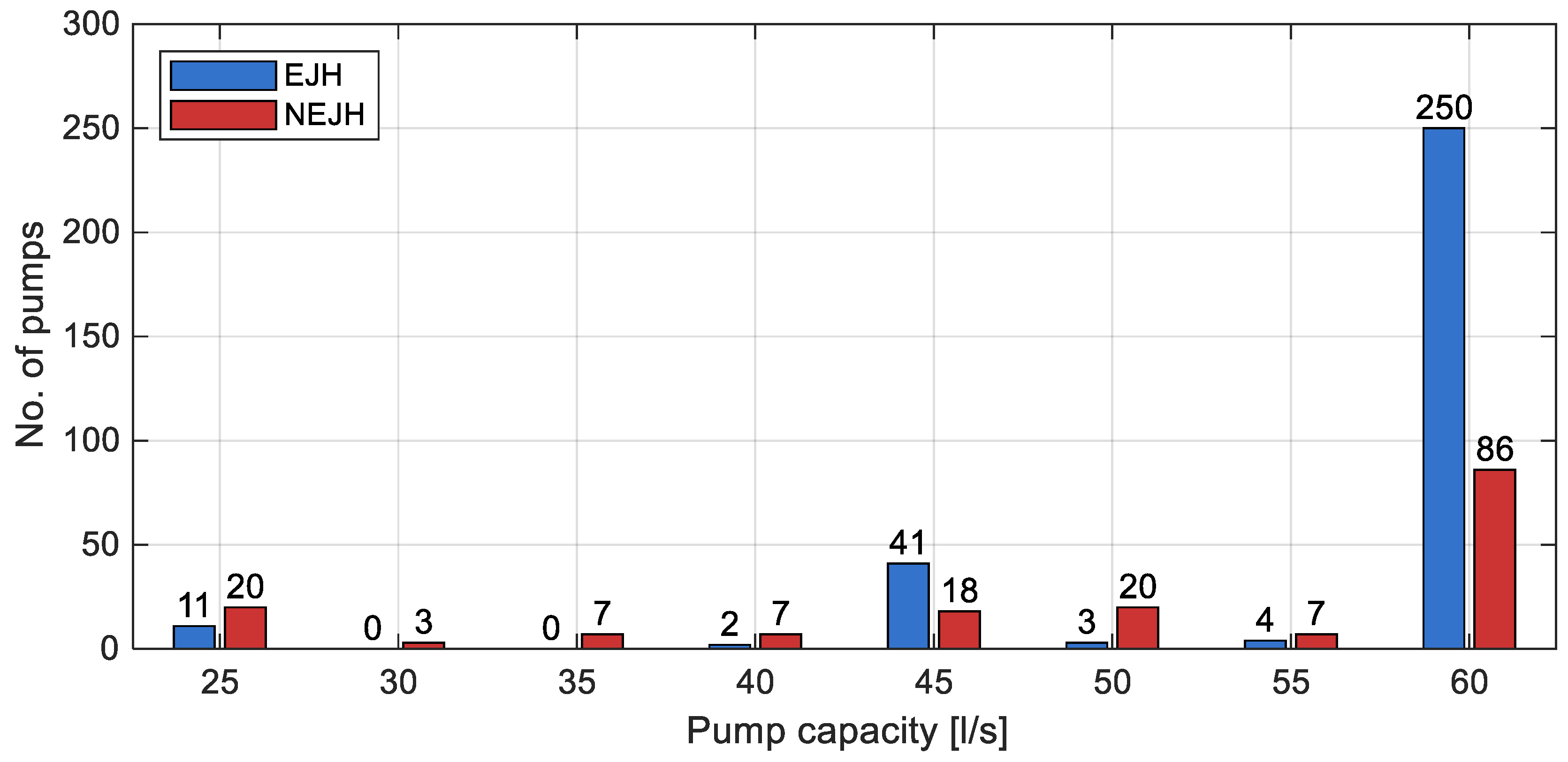
The capacities of the pumps installed in the EJH and NEJH well-fields range from 25 to 60 L/s. The number of pumps installed in the EJH and NEJH well-fields, depending on their capacity, is shown in Figure 6.

The diagram indicates an evident lack of uniformity in pump allocation. Low-capacity pumps (25–35 L/s) are relatively scarce in both fields, while mid-range pumps (40–55 L/s) show a moderate presence. The highest concentration is in the 60 L/s capacity class, where 250 pumps operate in the EJH well-field and 86 pumps in the NEJH well-field. This class overwhelmingly dominates the overall pump inventory, representing the main extraction capacity of the Jabal Hasouna WSS.

The nominal average capacity of the pumps at the EJH well-field is 56.495 L/s, while at the NEJH well-field it is 50.417 L/s. This results in an average nominal capacity of 54.363 L/s (equivalent to 4696.985 m³/day) for all installed pumps across both well-fields.

Overall, Figure 6 shows significant capacity asymmetry between the well-fields, with EJH having a higher total number of pumps and a notably larger share of high-capacity (60 L/s) pumps. This distribution is crucial for later reliability analysis, as the high failure impact and statistical weight of the 60 L/s pumps significantly affect system-level reliability metrics. The chance that a failed 60 L/s pump came from the EJH well-field is 0.7440, while the probability for the NEJH well-field is 0.5119. The overall probability that a failed pump (from either field) is 60 L/s is 0.7015. These results suggest that high-capacity (60 L/s) pumps should be prioritized in maintenance planning and resource allocation.

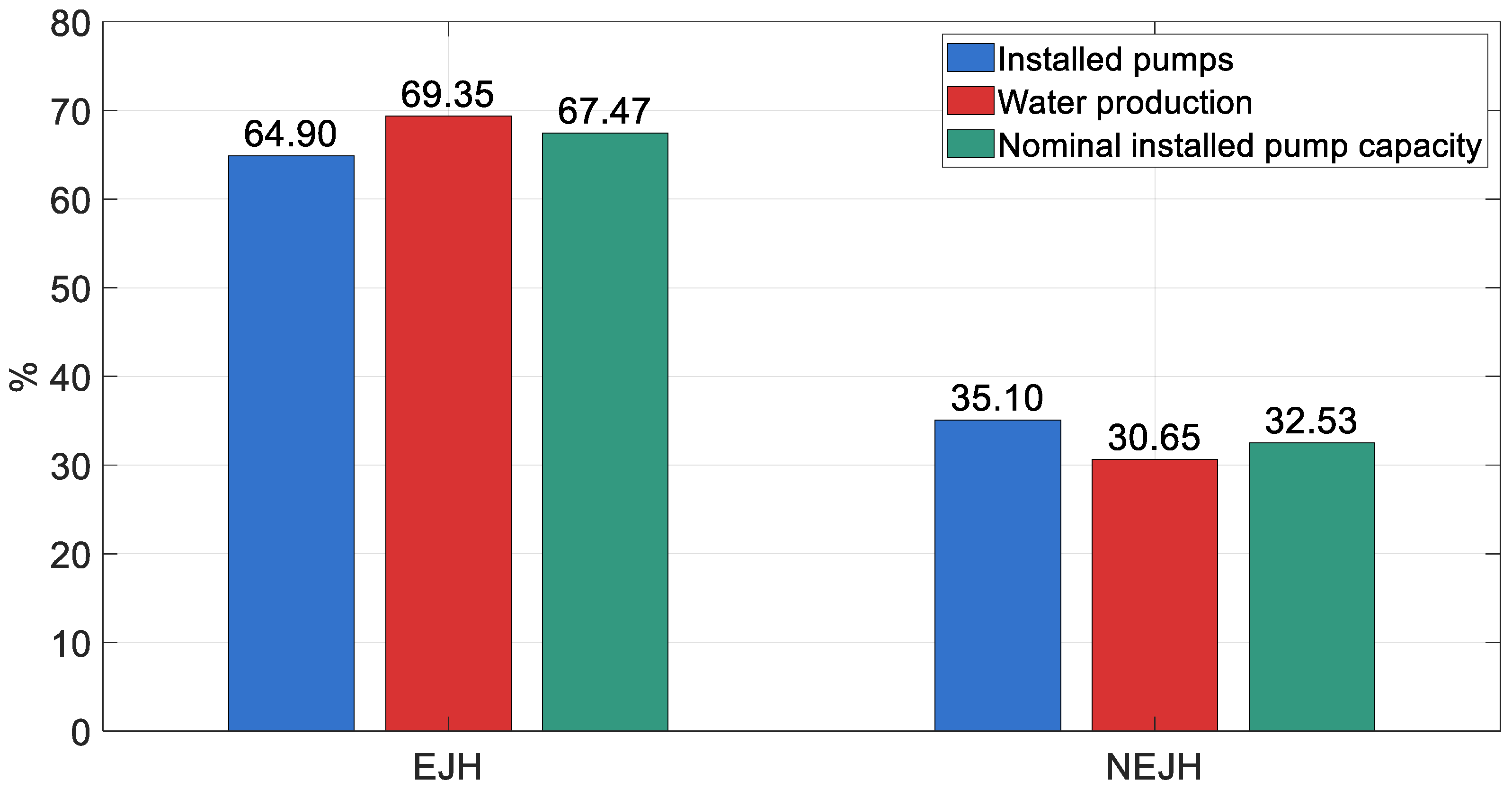
The diagram shown in Figure 7 illustrates the relative contributions of the EJH and NEJH well-fields to three key parameters of the Jabal Hasouna WSS: number of installed pumps (%), water production (%), and nominal installed pump capacity (%). Each parameter is expressed as a proportion of the total system value (EJH + NEJH = 100%).

For the EJH well-field, all three indicators surpass 60%, indicating that EJH, with 64.90% of installed pumps and 67.47% of nominal pump capacity, produces 69.35% of WSS output. This shows that EJH well-field hosts most of the pumping infrastructure and provides the majority of the actual water output. Water production slightly exceeds the proportion of installed pumps, implying higher average utilization or larger-capacity units in EJH compared to NEJH.

In contrast, the NEJH well-field contributes significantly less, with its share of installed pumps (35.10%) and nominal installed pump capacity (32.53%) being roughly proportional. However, its contribution to total water production (30.65%) is slightly lower than its installed capacity share, indicating comparatively lower operational efficiency or reduced utilization of the available pumping assets.

Overall, the diagram emphasizes a major functional and structural imbalance between the two well-fields, with EJH serving as the main production area of the Jabal Hasouna WSS, both in terms of infrastructure concentration and water volume supplied.

Table 1 shows data on water production (10⁶ m³/day), the number of operating weeks per year, the number of operating pumps, the average daily water production per pump (m³/day), and the pump utilization from 2005 to 2010 for the Jabal Hasouna WSS. Pump utilization is calculated by dividing the average daily water production per pump by the average nominal capacity of the pumps (4696.985 m³/day).

Table 1. Jabal Hasouna WSS production data.

Year	Water Production (106 m3/day)	No. of Operating Weeks	No. of Operating Pumps	Average Daily Water Production Per Pump (m3/day)	Utilization of the Pumps
2005	0.430023	29	113	3805.5133	0.8102
2006	0.553299	52	133	4160.1429	0.8858
2007	0.652556	52	186	3508.3656	0.7470
2008	0.701366	52	168	4174.7976	0.8889
2009	0.80119	52	191	4194.7120	0.8931
2010	1.047967	51	254	4125.8543	0.8785

Table 1. Jabal Hasouna WSS production data.

Year	Water Production (106 m3/day)	No. of Operating Weeks	No. of Operating Pumps	Average Daily Water Production Per Pump (m3/day)	Utilization of the Pumps
2005	0.430023	29	113	3805.5133	0.8102
2006	0.553299	52	133	4160.1429	0.8858
2007	0.652556	52	186	3508.3656	0.7470
2008	0.701366	52	168	4174.7976	0.8889
2009	0.80119	52	191	4194.7120	0.8931
2010	1.047967	51	254	4125.8543	0.8785

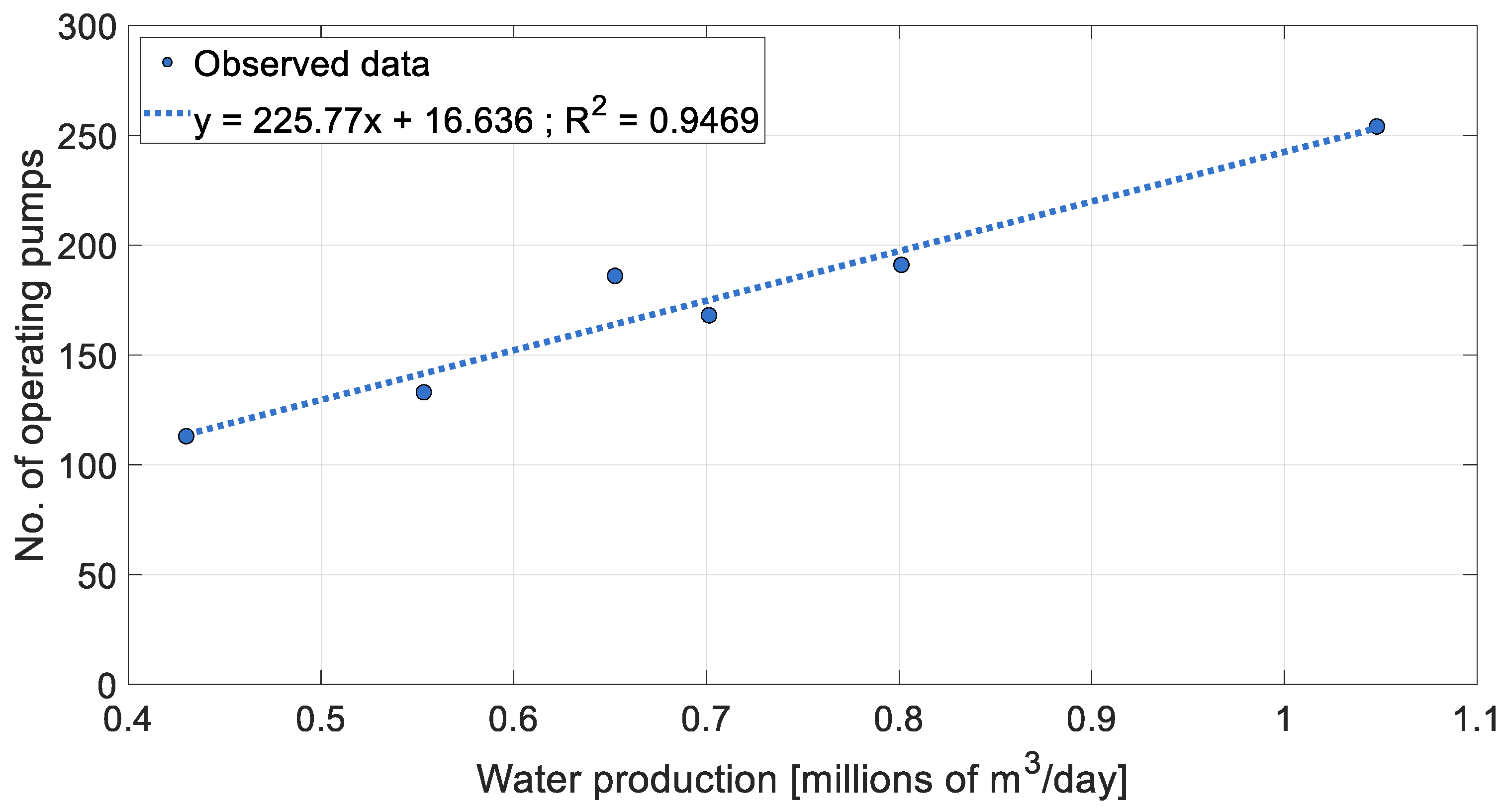
A strong linear correlation (R² = 0.9469) was identified between daily water production and the required number of operating pumps in the Jabal Hasouna WSS for the period 2005–2010 (see Figure 8).

Under ideal conditions, i.e., with pump utilization equal to 1, achieving the GMRP Phase II production capacity of 2.003 × 10⁶ m³/day would require 427 pumps out of the 479 installed. However, as the last column in Table 1 indicates, the actual pumps utilization is below one. To estimate the number of pumps needed to produce 2.003 million m³/day, the linear correlation equation from Figure 8 is applied. Since the pump configuration in terms of capacity is not specified (Table 1), the needed number of pumps can be estimated only by assuming that all pumps have the same capacity, i.e., Q_p (average daily water production per pump).

Finally, the number of pumps needed to produce 2.003 million m³/day is 469, corresponding to a pump utilization of η_p = 0.9093 and an average daily water production per pump of Q_p = 4270.7889 m³/day.

The assumption that all pumps have the same capacity is consistent with the requirements for applying the finite-source, multi-server queuing model with spares (Section 5.1), which assumes that all customers (pumps) requiring maintenance have identical characteristics, i.e., identical capacities. Thus, the number of pumps required to operate is M = 469 (out of N = 479 installed), leaving a maximum of Y = 10 pumps available as standby (spare) units.

4.2. Determination of Pump Reliability and Failure Intensity

For the analysis of failure intensity, failures from all pumps (data structure shown in Figure 3) were considered, regardless of their operating location (field). When viewed by year, the number of pumps in operation during the observed period varied. To determine failure intensity more accurately, the number of pumps in operation during the observed period will be calculated as the expected (mean) number of pumps operating during that time. The number of operating weeks and number of pumps in operation per year during the observed period are shown in Table 1 (columns 3 and 4 respectively).

Expected (mean) number of pumps operating during the observed period is

$${\overline{N}}_p={\displaystyle \frac{1}{288}}\cdot (29\cdot 113+52\cdot 133+52\cdot 186+52\cdot 168+52\cdot 191+51\cdot 254)=178.77~179 \mathrm{pumps}$$

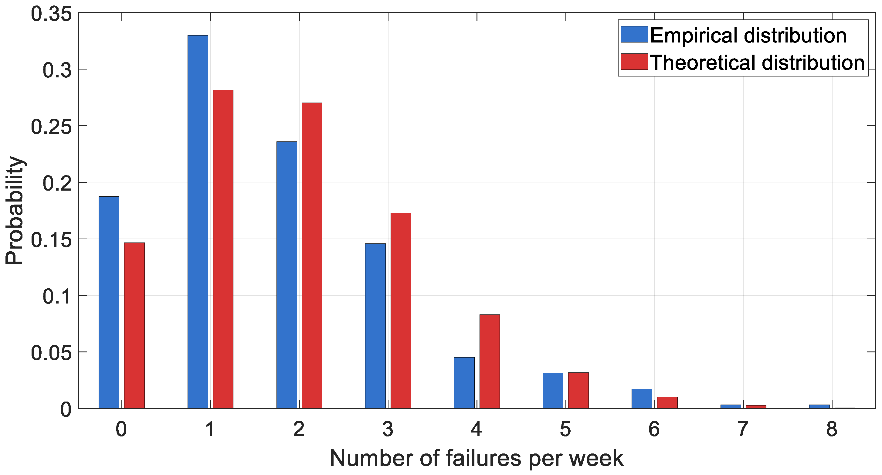
The number of failures of all pumps was analyzed on a weekly interval. By analyzing the failure data of the pumps and applying the K-S test (p-value = 0.01) [33], it was found that the number of failures of all pumps in operation per week follows a Poisson distribution with parameter α = 1.9191, as shown in the diagram in Figure 9. The parameter α of the obtained Poisson distribution represents the failure intensity—λ of the 179 pumps that are operating on average over a one-week period. This also means that the time between pump failures is exponentially distributed with the same failure intensity.

For the purposes of further analysis, the failure intensity will be expressed per pump and per day, meaning that the obtained failure intensity needs to be divided by 179 to get the failure intensity per one working pump and by 7 to get the failure intensity per day. Finally, the failure intensity of one pump per day is

λ = 0.00153152434158 failures/pump/day, i.e., 1/day

(1)

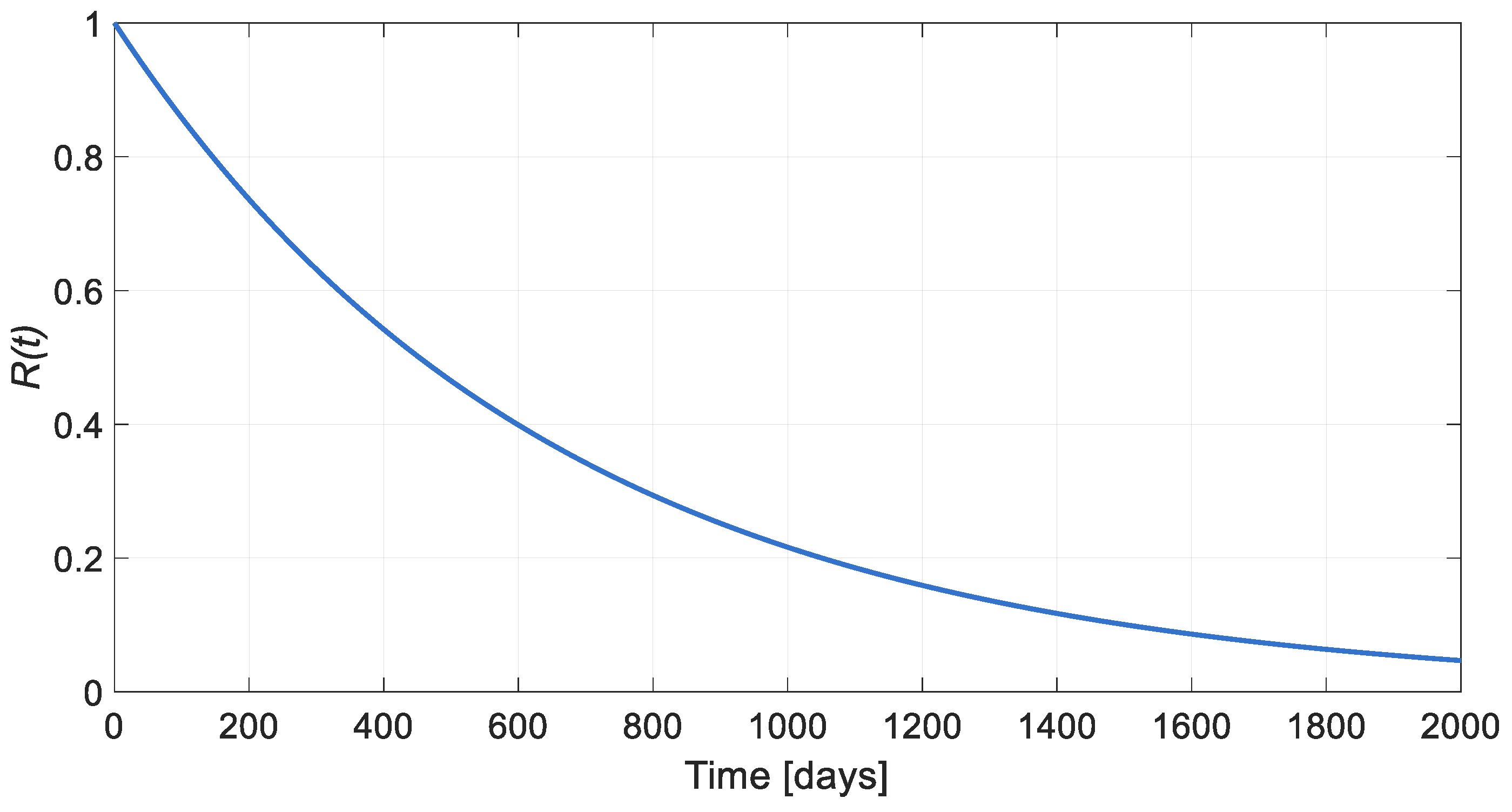
According to the bathtub curve, constant failure intensity means that pumps are in the second period of the life cycle, exploitation, where their reliability is exponentially distributed [34], Figure 10.

4.3. Analysis of Pump Failure Duration—Determination of Overall Maintenance Intensity

Mechanical, electrical, and electronic components (telecommunication) are the primary sources of pump failures. Mechanical components include submersible well pumps and wellhead valves, such as blow-down valves, air vacuum relief valves, lateral valves, and non-slam check valves. Electrical components include submersible well pump motors, components for the distribution panel for wellhead motor control, pressure transmitters, flow switches, power cables, and other related elements. Electronics and telecommunications involve flow elements, components related to the wellhead control panel, programmable logic controller software, faults, electronic boards, and more.

The maintenance system is decentralized (see Appendix A), with maintenance personnel trained to address all three types of failures. They also conduct preventive maintenance for electrical and electronic components, including activities such as valve maintenance, transformer maintenance, and battery replacements that do not affect pump operation. The adopted maintenance strategy is “wait and see,” meaning that pumps operate until failure, and periodic inspections do not disrupt pump operation [7].

Determination of pumps’ corrective maintenance (CM) intensity—analysis of failure duration

In the analysis of failure duration, all types of failures were considered together, primarily due to the organization of the maintenance system and the size of the available sample. The classification of failures was initially done based on the duration of the failure, as follows (Main failure types):

• “Standard” failures: It was empirically determined that all failures requiring less than 48 h to fix and not requiring the pump to be removed from the site belong to this group. In the second step, “standard” failures were further divided by location, i.e., the field or part of the field where the pumps are located. One reason for this classification is the varying distance of the fields or parts of the fields where the pump failure occurred from the central workshop, the place where maintenance workers (mobile teams) who are responsible for fixing the failures are located.
• Catastrophic failures: For this group, the time required to repair the failure exceeds 48 h, and the pump is removed from the site. Furthermore, catastrophic failures are divided into those that can be repaired in the workshop by maintenance staff (Type 1) and those for which the pump must be transported to the manufacturer (Type 2). Due to the relatively small number of these failures and the long time required to repair them, failures of this type from all fields were considered together.

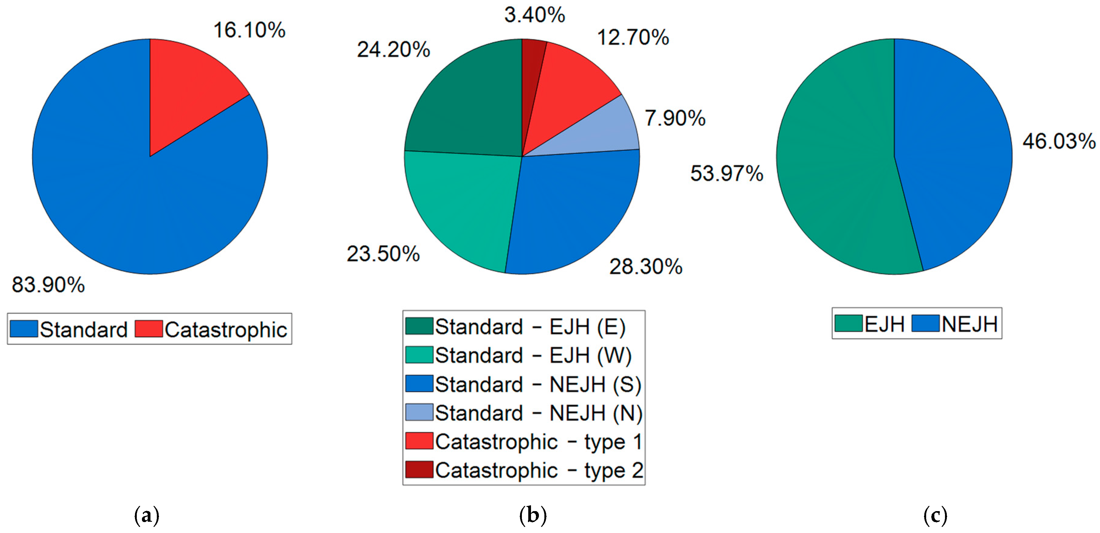
The diagram in Figure 11a shows the share of main failure types in the total number of failures during the observed period, while the diagram in Figure 11b shows the share of standard failures distributed across pump fields, as well as the share of catastrophic failures (Type 1 and Type 2), also during the observed period.

Also, the Kolmogorov–Smirnov (K-S test) goodness-of-fit test is used for determining whether each of six samples of failure durations (see Figure 11b) belongs to a hypothesized theoretical distribution, with p-value = 0.01.

Figure 11c shows the share of the number of failures due to the place of origin, i.e., EJH or NEJH well-field. Even though EJH well-field has 311 installed pumps, 1.851 times more than NEJH well-field, the number of failures is close.

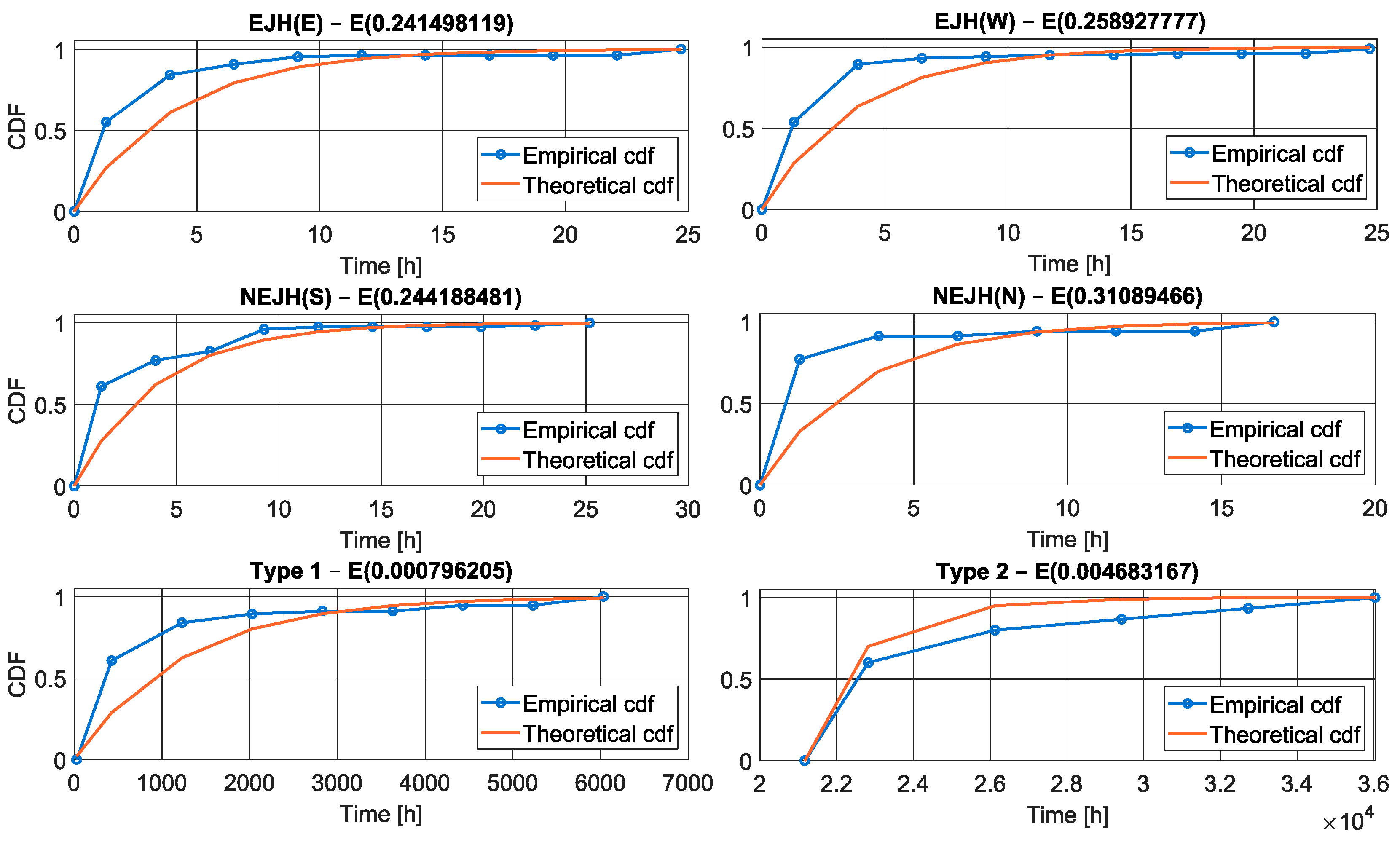
The resulting theoretical distributions of the failure durations (repair times), depending on the pump field (standard failures) and the type of catastrophic failures, are shown in Figure 12, where E(α) represents an exponential distribution with parameter α. Parameter α, in this case, represents the so-called maintenance intensity (μ) for each standard and catastrophic type of pump failure.

Maintenance intensities (per hour) for the case of standard-duration failures, depending on the location of occurrence (field), are as follows (Figure 12):

-

μ_EJH(E) = 0.241498119 1/h, for well-field EJH(E);

-

μ_EJH(W) = 0.258927777 1/h, for well-field EJH(W);

-

μ_NEJH(S) = 0.244188481 1/h, for well-field NEJH(S);

-

μ_NEJH(N) = 0.31089466 1/h, for well-field NEJH(N).

The maintenance intensities in the case of catastrophic failures are as follows:

-

μ_type1 = 0.000796205 1/h, for catastrophic failures of Type 1;

-

μ_type2 = 0.004683167 1/h, for catastrophic failures of Type 2.

The average maintenance intensity (μ_CM) for CM, which takes into account all types of standard failures, both types of catastrophic failures, as well as their shares in the total number of failures during the observed period (see Figure 11b), can be determined as

$$\begin{gathered} {\mu }_{CM}=0.242\cdot {\mu }_{EJH(E)}+0.235\cdot {\mu }_{EJH(W)}+0.283\cdot {\mu }_{NEJH(S)}+0.079\cdot {\mu }_{NEJH(N)}+\dots \\ +0.127\cdot {\mu }_{type1}+0.034\cdot {\mu }_{type2} \end{gathered}$$

Finally, the average maintenance intensity for CM is

μ_CM = 0.213322389 1/h.

For the purposes of further analysis, the average maintenance intensity will be expressed per day, meaning that the obtained average maintenance intensity needs to be multiplied by 24, which finally results in

μ_CM = 5.119737336 1/day.

Frequency and duration of preventive maintenance (PM) activities

PM is performed only on specific parts of the system, such as step-down transformers (oil replacement, insulation check, loss measurement, etc.) and non-slam check valves (valve inspection, cleaning, possible replacement, etc.), and it is planned in advance. PM is carried out when a component (part) reaches a certain number of operating hours or according to a fixed date. In other words, this means that the performance of PM activities is not considered to be influenced by stochastic factors.

Since the execution of PM is deterministic, its impact on the functioning of the overall maintenance system will be expressed through the average time per day required to perform PM activities. In practical terms, this means that the available time for performing CM activities during the day is reduced by the amount of time needed to carry out PM. It is important to note that CM activities have absolute priority over PM activities.

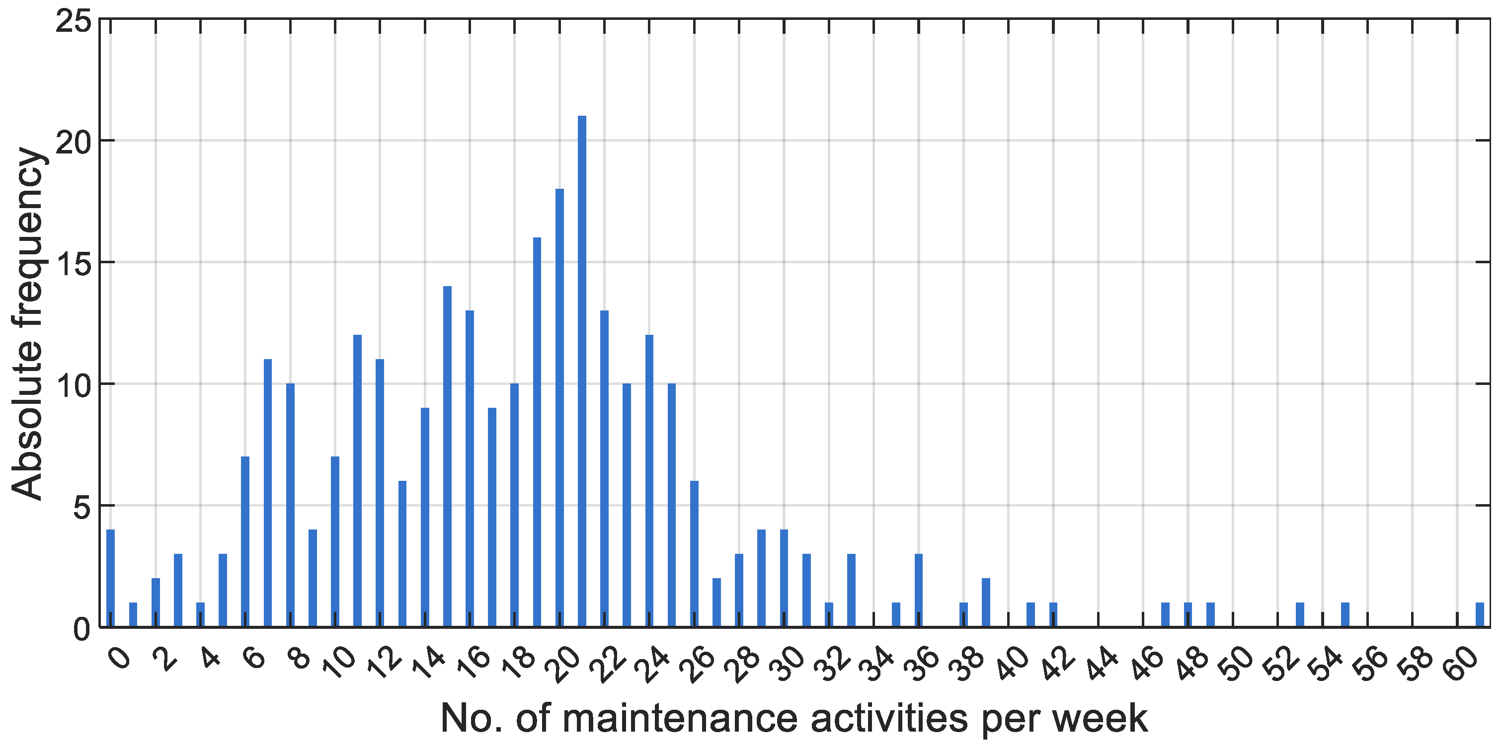
The frequency of PM activities performed on step-down transformers on a weekly basis during the observed period is shown in the diagram in Figure 13.

As can be seen from Figure 13, the number of activities is in the range of 0 to 60; most frequently, the number of activities is 21, while the dominant value range is between 10 and 25 weekly activities. The analysis of step-down transformer maintenance activities reveals a stable pattern, with a moderate number of interventions in most weeks. The extreme values (e.g., 50, 60 activities) may be a result of a backlog of delayed maintenance tasks.

The average number of PM activities per week related to step-down transformers is

$${\overline{N}}_{sdt}^{week}=18.43525 \mathrm{activities}/\mathrm{week}$$

Alternatively, the average number of PM activities per day is

$${\overline{N}}_{sdt}^{day}=2.633607 \mathrm{activities}/\mathrm{day}$$

The average duration of one PM activity related to step-down transformers during the observed period is

$${\overline{t}}_{sdt}^{actvity}=0.214121 \mathrm{h}/\mathrm{activity}$$

Finally, the average duration of PM activities related to step-down transformers during the observed period per day is

$${\overline{t}}_{sdt}^{day}=0.563911 \mathrm{h}/\mathrm{day}$$

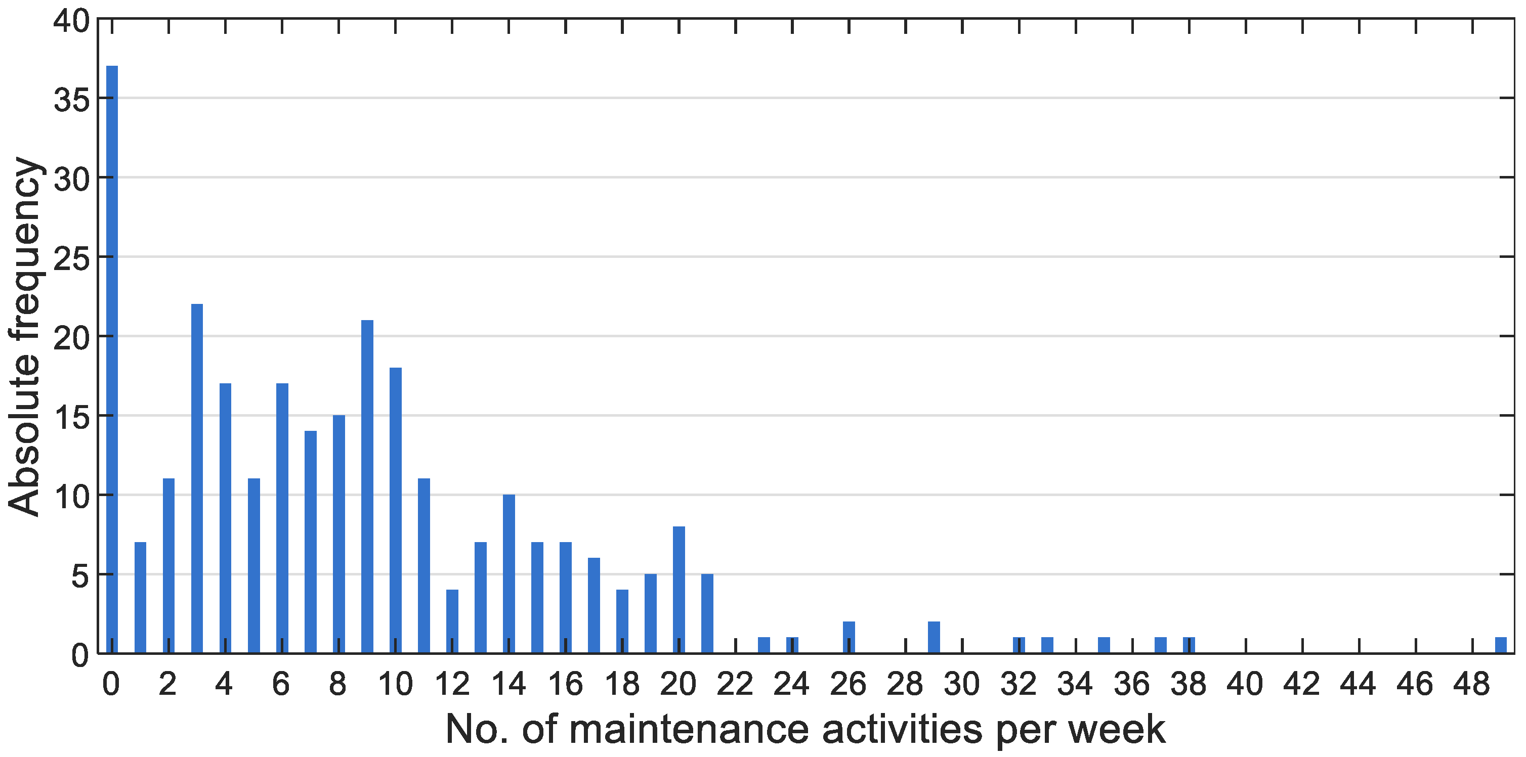
The frequency of PM activities performed on the non-slam check valve on a weekly basis during the observed period is shown in the diagram in Figure 14.

As can be seen from Figure 14, the most frequent value is 0 activities, occurring in over 35 weeks, indicating that most weeks pass with no maintenance. The frequency decreases significantly as the number of maintenance activities increases, and most maintenance activity counts fall within the range of 0 to 15 per week. There are a few isolated weeks with extremely high maintenance counts (e.g., 32, 33, 35, 37, 38, and 49), each occurring only once, which likely result from specific operational conditions, scheduled overhauls, backlog accumulation from previous delays, etc.

The average number of PM activities per week related to non-slam check valves is

$${\overline{t}}_{PM}^{day}=8.836957 \mathrm{activities}/\mathrm{week}$$

Alternatively, the average number of PM activities per day is

$${\overline{N}}_{ncv}^{day}=1.26242 \mathrm{activities}/\mathrm{day}$$

The average duration of one PM activity related to non-slam check valves during the observed period is

$${\overline{t}}_{ncv}^{actvity}=0.512147 \mathrm{h}/\mathrm{activity}$$

Finally, the average duration of PM activities related to non-slam check valves during the observed period per day is

$${\overline{t}}_{ncv}^{day}=0.646546 \mathrm{h}/\mathrm{day}$$

Overall duration of PM activities, i.e., the total average time per day spent on PM activities related to step-down transformers and non-slam check valves is

$${\overline{t}}_{PM}^{day}={\overline{t}}_{sdt}^{day}+{\overline{t}}_{ncv}^{day}=0.563911+0.646546=1.210457 \mathrm{h}/\mathrm{day}$$

Determination of overall average maintenance intensity for CM (μ)

The determination of the overall average maintenance intensity for CM considers the average maintenance intensity for CM and the overall duration of PM activities.

The maintenance subsystem works 24 h a day, 7 days a week, and if we take into consideration only CM, then the average maintenance intensity for CM per day is

μ_CM = 5.119737336 1/day

Due to the fact that the available time for performing CM during the day is reduced by the amount of time needed to carry out PM activities ${\overline{t}}_{PM}^{day}$, which is 1.210457 h/day, the available time for CM per day is reduced to 22.789543 h. Accordingly, average maintenance intensity for CM also has to be reduced. This leads to the so-called overall average maintenance intensity for CM − μ, whose value is

μ = 4.861519757 1/day

(2)

5. Determining Operating Parameters of WSS

The model for determining operating parameters (KPIs) of WSS is based on queuing theory, multi-server finite-source with spare parts model, i.e., machine-repair model [35,36]. Reliability of WSS (R_wss) and lost water production ($Q_{lw}^{day}$) due to pump failures represent the most critical operating parameters (KPIs) of the WSS in the context of risk assessment.

5.1. Model of a Finite-Source, Multi-Server Queuing System with Spares (M/M/c//N/Y)

The queuing model to be presented has the repair teams as its servers and the machines requiring repair as its customers, which can be in operating mode or in standby mode (i.e., idle). With one slight exception, this system fits the classical finite-source, multi-server queuing system—M/M/c//N. [35,36]

The Multi-server Finite-Source with Spare Parts queuing model determines, among other things, the system’s state probabilities, i.e., the probabilities that a given number of machines have failed. These probabilities are determined based on the total number of machines (N)—source; required number of operational machines (M) for the system to function; the number of machines in “stand-by” mode (Y)—spares; the failure intensity per individual machine (λ); the service intensity of each server—repair team (μ); and the number of servers—repair teams (c). In our case, the machines are pumps.

In most cases, machine maintenance (repair) within the organizational structure of a manufacturing, transportation, or service company, etc., represents a subsystem whose primary function, within its area of responsibility, is to enable the “Main System” to fulfill the purpose and tasks for which it exists.

The most important application of the M/M/c//N model has been in the machine repair (maintenance) subsystem, where one or more maintenance crew members are responsible for keeping a group of N machines operational by repairing each one that fails. Maintenance operators are treated as individual servers in the queuing system if they work independently on different machines, whereas the entire crew is treated as a single server if crew members work together on each machine.

The machines constitute the customer population. Each one is considered a customer in the queuing system when it is down, waiting to be repaired, whereas it is outside the system while it is operational. Each member of the customer population alternates between being inside and outside the queuing system.

This slight exception, in which this model differs from the M/M/c//N model, is reflected in the fact that not all N machines work simultaneously, but a certain number of them are in standby mode and represent spare machines (they are not engaged and cannot fail). Their role is to start operating when one of the machines in operation fails, that is, to switch from standby mode to operational mode.

For the model of the M/M/c//N/Y queuing system, let N denote the total customer population (i.e., the total number of machines), Y represent the portion of the population that cannot generate service requests (N > Y, corresponding to the number of spare machines in standby mode), and c denote the number of servers (N > c). The following assumptions are made:

-

All customers (machines) are the same and have the same constant mean arrival rate to the queuing system (failure intensity) λ, and the time between arrivals (failures) follows an exponential distribution.

-

The mean service rate (service intensity) μ is identical and constant for all servers and follows an exponential distribution.

-

Customers (machines) are served (repaired) based on the First-In, First-Out (FIFO) discipline.

-

When all servers are busy, the failed machine joins the queue and waits to be served (repaired).

The state of the M/M/c//N/Y queuing system, maintenance subsystem k (k = 0, …, N), is determined based on the number of machines that have failed. The mean transition intensities of the maintenance subsystem from one state to another depend on its current state, and in the case of machine failures (arrivals to the queuing system), they are

$${\lambda }_k=\left\{\begin{array}{l}(N-Y)\cdot \lambda ; 0\le k\le Y\\ (N-k)\cdot \lambda ; Y+1\le k\le N\end{array}\right.$$

(3)

while in the case of machine repairs (departures from the queuing system), they are

$${\mu }_k=\left\{\begin{array}{l}k\cdot \mu ; 0\le k\le c\\ c\cdot \mu ; c+1\le k\le N\end{array}\right.$$

(4)

The probabilities that the maintenance subsystem will be in one of the possible states p_k (k = 0, …, N) in the stationary regime are determined by the following system of algebraic equations:

$$\begin{gathered} 0:\hspace{0.33em}{\lambda }_0\cdot p_0+{\mu }_1\cdot p_1=0, \\ k:\hspace{0.33em}{\lambda }_{k-1}\cdot p_{k-1}-({\lambda }_k+{\mu }_k)\cdot p_k+{\mu }_{k+1}\cdot p_{k+1}=0,k=1,\dots ,N-1 \\ N:\hspace{0.33em}{\lambda }_{N-1}\cdot p_{N-1}-{\mu }_N\cdot p_N=0, \end{gathered}$$

(5)

with the additional condition:

$${\displaystyle \sum _{k=0}^N{p}_k=1}$$

The server utilization, ρ, can calculated as

$$\rho ={\displaystyle \frac{\overline{\lambda }}{c\cdot \mu }}$$

(6)

where $\overline{\lambda }$ is the average arrival rate of customers (machines) to the queuing system, i.e., the average failure intensity, and it can be calculated as

$$\overline{\lambda }={\displaystyle \sum _{k=0}^N{\lambda }_k\cdot p_k}$$

The expected number of machines in the queuing system, i.e., the machines that have failed (L), can be calculated as

$$L={\displaystyle \sum _{k=0}^{N}k\cdot p_k}$$

(7)

whereas the expected number of machines that are waiting for service (repair), denoted by (L_q), is determined as

$$L_q={\displaystyle \sum _{k=c+1}^N(k-c)\cdot p_k}$$

(8)

The expected number of failed machines (L′) that affect the normal functioning of “Main System” can be calculated as

$$L^{\prime }={\displaystyle \sum _{k=Y+1}^N(k-Y)\cdot p_k}$$

(9)

5.2. Evaluation of WSS Reliability and Associated Lost Water Production

In this case, reliability refers to the probability that the “Main System”, WSS, will be able to deliver the required amount of water, i.e., that the number of pumps (machines) necessary for providing the required amount of water will be operational. The WSS is unable to deliver the necessary quantity of water when the number of failed pumps (k) is equal to the number of pumps in “stand-by” mode plus one (Y + 1).

Accordingly, the most significant state and its probability is one when the queuing system (maintenance subsystem) is in the state Y + 1, i.e., P[k = Y + 1]. The state in which Y + 1 pumps have failed represents a risk event, while the corresponding probability presents the probability of occurrence of the risk event.

By subtracting the probability that the maintenance subsystem of the WSS is in state Y + 1 from one, the desired WSS reliability is obtained. In this way, the reliability that the WSS will fulfill its task can be determined as

$$R_{wss}=1-P\left[k=Y+1\right]$$

(10)

Lost water production (m³ per day) can be determined as the product of the expected number of failed machines that affect normal functioning of WSS (L′) and average daily production per pump (Q_p):

$$Q_{lw}^{day}=L^{\prime }\cdot Q_p$$

(11)

KPIs of WSS, as well as the reliability of the WSS (R_wss) and the associated lost water production ($Q_{lw}^{day}$), calculated using (10) and (11), are used as partial indicators in the assessment of WSS risk (R) defined by (12).

5.3. Calculation of WSS Operating Parameters (KPIs)

The objective of evaluating the WSS operating parameters (KPIs) required to achieve the target production level of 2.003 million m³/day from the EJH and NEJH well-fields (Phase II), among others, is to derive partial indicators for system risk assessment. The considered KPIs include the expected number of failed pumps (L)—defined by expression (7); the expected number of failed pumps that affect required water production (L′)—defined by expression (9); lost water production m³ per day ($Q_{lw}^{day}$)—defined by expression (11); and the reliability of the WSS (R_wss)—defined by expression (10). These operating parameters (KPIs) are derived using an M/M/c//N/Y queuing theory model, based on the following input data (independent variables):

-

Total number of installed pumps, N = 479;

-

Required number of operational pumps, M = 469;

-

Number of pumps in “stand-by” mode, Y = 0, 1, 2, …, 10 (see last paragraph, Section 4.1.);

-

Number of servers—field repair teams, c = 1,2,3 (see Appendix A);

-

Pumps failure intensity, λ = 0.00153152434158 1/day (1);

-

Service intensity per server—field repair team, μ = 4.861519757 1/day (2).

Numerical values of considered KPIs are shown in

Table 2. Operating parameters of WSS (c = 1).

M = 469 Pumps		II Phase Capacity: 2.003 × 106 m3/day		c = 1
Y	Rwss	L (Pumps)	L′ (Pumps)	${\mathit{Q}}_{\mathit{l}\mathit{w}}^{\mathit{d}\mathit{a}\mathit{y}}$(m3/day)
0	0.87407	L(Y = 0) = 0.17321	1.7321 × 10−1	7.3976 × 102
1	0.98140	L(Y = 0) + 1.19 × 10−4	2.5591 × 10−2	1.0929 × 102
2	0.99725	L(Y = 1) + 2.56 × 10−5	3.7810 × 10−3	1.6148 × 101
3	0.99959	L(Y = 2) + 4.97 × 10−6	5.5863 × 10−4	2.3858
4	0.99994	L(Y = 3) + 9.10 × 10−7	8.2538 × 10−5	3.5250 × 10−1
5	1 − 8.87 × 10−6	L(Y = 4) + 1.60 × 10−7	1.2195 × 10−5	5.2082 × 10−2
6	1 − 1.31 × 10−6	L(Y = 5) + 2.76 × 10−8	1.8018 × 10−6	7.6950 × 10−3
7	1 − 1.94 × 10−7	L(Y = 6) + 4.64 × 10−9	2.6621 × 10−7	1.1369 × 10−3
8	1 − 2.86 × 10−8	L(Y = 7) + 7.69 × 10−10	3.9332 × 10−8	1.6798 × 10−4
9	1 − 4.22 × 10−9	L(Y = 8) + 1.26 × 10−10	5.8113 × 10−9	2.4819 × 10−5
10	1 − 6.24 × 10−10	L(Y = 9) + 2.05 × 10−11	8.5862 × 10−10	3.6670 × 10−6

,

Table 3. Operating parameters of WSS (c = 2).

M = 469 Pumps		II Phase Capacity: 2.003 × 106 m3/day		c = 2
Y	Rwss	L (Pumps)	L′ (Pumps)	${\mathit{Q}}_{\mathit{l}\mathit{w}}^{\mathit{d}\mathit{a}\mathit{y}}$(m3/day)
0	0.87258	L(Y = 0) = 0.14851	1.4851 × 10−1	6.3424 × 102
1	0.99059	L(Y = 0) + 4.70 × 10−5	1.0971 × 10−2	4.6853 × 101
2	0.99930	L(Y = 1) + 5.20 × 10−6	8.1045 × 10−4	3.4613
3	0.99995	L(Y = 2) + 5.12 × 10−7	5.9871 × 10−5	2.5570 × 10−1
4	1 − 3.80 × 10−6	L(Y = 3) + 4.73 × 10−8	4.4230 × 10−6	1.8890 × 10−2
5	1 − 2.80 × 10−7	L(Y = 4) + 4.19 × 10−9	3.2675 × 10−7	1.3955 × 10−3
6	1 − 2.07 × 10−8	L(Y = 5) + 3.61 × 10−10	2.4138 × 10−8	1.0309 × 10−4
7	1 − 1.53 × 10−9	L(Y = 6) + 3.05 × 10−11	1.7832 × 10−9	7.6156 × 10−6
8	1 − 1.13 × 10−10	L(Y = 7) + 2.53 × 10−12	1.3173 × 10−10	5.6260 × 10−7
9	1 − 8.35 × 10−12	L(Y = 8) + 2.08 × 10−13	9.7320 × 10−12	4.1562 × 10−8
10	1 − 6.17 × 10−13	L(Y = 9) + 1.70 × 10−14	7.1900 × 10−13	3.0704 × 10−9

and

Table 4. Operating parameters of WSS (c = 3).

M = 469 Pumps		II Phase Capacity: 2.003 × 106 m3/day		c = 3
Y	Rwss	L (Pumps)	L′ (Pumps)	${\mathit{Q}}_{\mathit{l}\mathit{w}}^{\mathit{d}\mathit{a}\mathit{y}}$(m3/day)
0	0.87254	L(Y = 0) = 0.14772	1.4773 × 10−1	6.3091 × 102
1	0.99058	L(Y = 0) + 4.34 × 10−6	1.0414 × 10−2	4.4476 × 101
2	0.99954	L(Y = 1) + 3.23 × 10−6	5.1288 × 10−4	2.1904
3	0.99998	L(Y = 2) + 2.13 × 10−7	2.5259 × 10−5	1.0788 × 10−1
4	1 − 1.12 × 10−6	L(Y = 3) + 1.31 × 10−8	1.2440 × 10−6	5.3129 × 10−3
5	1 − 5.54 × 10−8	L(Y = 4) + 7.78 × 10−10	6.1267 × 10−8	2.6166 × 10−4
6	1 − 2.73 × 10−9	L(Y = 5) + 4.47 × 10−11	3.0174 × 10−9	1.2887 × 10−5
7	1 − 1.34 × 10−10	L(Y = 6) + 2.52 × 10−12	1.4861 × 10−10	6.3466 × 10−7
8	1 − 6.62 × 10−12	L(Y = 7) + 1.40 × 10−13	7.3190 × 10−12	3.1257 × 10−8
9	1 − 3.26 × 10−13	L(Y = 8) + 7.99 × 10−15	3.6000 × 10−13	1.5394 × 10−9
10	1 − 1.60 × 10−14	L(Y = 9) + 0.00	1.8000 × 10−14	7.5815 × 10−11

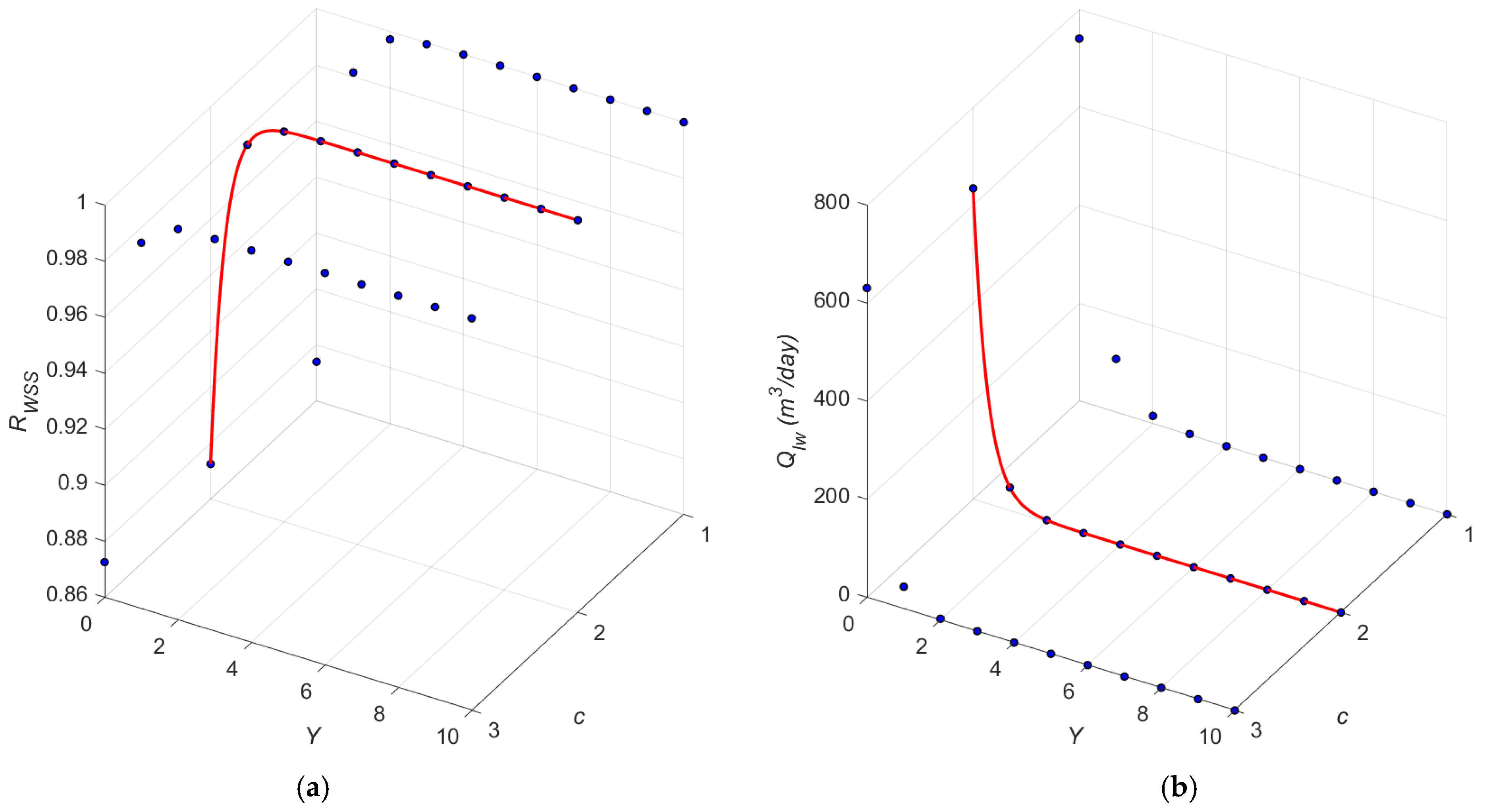
, depending on the number of servers—field repair teams (c), respectively, while the change of WSS reliability and lost water production are also shown in Figure 15.

6. Model for WSS Risk Assessment

The risk assessment of the WSS refers to a risk event defined as the inability of WSS to deliver the required 2.003 millions of m³ of water per day. For various WSS configurations (N, c, and Y), the risk (R) is quantified according to its definition—the product of two components; partial indicators—the occurrence of risk event (p); and the severity of consequences (C), which are generated by the risk event [17]

R = p × C

(12)

In this study, the risk partial indicators are ranked on a scale from 1 to 5, resulting in final WSS risk values that fall within the interval [1,25]. Based on this range, a standard three-level risk classification is proposed [37]:

• Tolerated risk: 1–3;
• Controlled risk: 4–12;
• Unacceptable risk: 15–25.

6.1. Criterion Scale for Evaluating the Occurrence of the Risk Event

Reliability of WSS, R_wss, defined by expression (9) and shown in Figure 15a, is used as a criterion for evaluating the occurrence of a risk event. The proposed and used criterion scale for determining risk event occurrence—p and its rank is presented in

Table 5. Criterion scale for determining risk event occurrence.

Criterion—Rwss	Occurrence of Risk Event—p	Rank
$R_{wss}>0.99$	Very Low	1
$0.95<R_{wss}\le 0.99$	Low	2
$0.90<R_{wss}\le 0.95$	Medium	3
$0.80<R_{wss}\le 0.90$	High	4
$R_{wss}\le 0.80$	Very High	5

.

6.2. Criterion Scale for Evaluating the Severity of Consequences of the Risk Event

The study by Boryczko et al. [37] suggested that the criteria for evaluation of the severity of consequences (C), in risk assessment for WSS, should be the number of consumers who are affected by water delay insufficiency. In Libya, the daily average water consumption per capita is 255 L/day [38]. Knowing the amount of lost water production caused by the occurrence of the risk event $Q_{lw}^{day}$, defined by expression (10) and shown in Figure 15b, allows for the calculation of affected customers—number of consumers which will be left without water—N_c as

$$N_c={\displaystyle \frac{Q_{lw}^{day}\hspace{0.17em}[\frac{m^3}{day}]}{0.255\hspace{0.17em}[\frac{m^3}{day}]}}$$

(13)

The proposed criterion scale, used in this study, for determining the severity of consequences C and its rank is presented in

Table 6. Criterion scale for determining the severity of consequences. [37].

Criterion—Nc	Severity of Consequences—C	Rank
$N_c\le 100$	Very Low	1
$100<N_c\le 500$	Low	2
$500<N_c\le 2000$	Medium	3
$2000<N_c\le 5000$	High	4
$N_c>5000$	Very High	5

.

6.3. Risk Assessment of WSS

Having all previously stated in mind, the assessed risk (R) for different configurations of the WSS (c—number of servers—field repair teams and Y—number of pumps in “stand-by” mode), is shown in

Table 7. Assessed risks (R) for different WSS configurations.

Y	c = 1	c = 2	c = 3
0	16	16	16
1	4	2	2
2	1	1	1
3	1	1	1
4	1	1	1
>4	1	1	1

.

7. Discussion of Obtained Results and Determination of the Best WSS Configuration

The results presented in Table 3, Table 4 and Table 5 will be discussed first. Across all three tables (c = 1, 2, 3), the reliability of the WSS (R_wss) increases rapidly with the number of standby pumps Y, approaching almost perfect reliability when Y ≥ 3. For c = 1, R_wss increases from 0.874 at Y = 0 to 0.9996 at Y = 3, meaning that even a small number of standby pumps significantly mitigates the effect of having only one field repair team, while for c = 2 and c = 3, reliability improves even faster, reaching R_wss ≈ 0.9993 at Y = 2, and exceeds 0.99997 at Y ≥ 3. Increasing the number of standby pumps provides redundancy, making the system far more resilient to pump failures. The presence of additional field repair teams (higher c) accelerates reliability improvement, as failed pumps are repaired more quickly and do not accumulate in the maintenance subsystem.

Both L (expected number of failed pumps) and L′ (expected number of failed pumps that affect required water production) show strong diminishing returns as Y increases. At Y = 0, L is around 0.17 (c = 1) and 0.148 (c = 2, 3). Higher c yields slightly lower L because repair capacity is larger. When Y increases from 0 to 1, L′ is significantly affected (0.173 → 0.0256 for c = 1), indicating a reduction in water loss. For Y ≥ 3, L′ becomes extremely small (below 10⁻⁴), meaning additional standby pumps have almost no impact on water production. The majority of the water production benefit is achieved with the first 1–2 standby pumps. Beyond Y = 3, the WSS is practically saturated in terms of improvement, i.e., failures that affect water production are so rare and repair times are so short that additional standby capacity has a negligible effect.

The lost water production $Q_{lw}^{day}$ (m³/day) decreases exponentially with Y for all three values of c. For c = 1, lost production is high at Y = 0 (~740 m³/day) but drops to near zero (<0.00001 m³/day) at Y ≥ 7. With c = 2, the initial loss at Y = 0 is lower (634 m³/day) due to a higher repair rate, and the reduction is faster. For c = 3, the lost water production at Y = 0 is almost identical to the case when c = 2, but the decline is even steeper. Finally, increasing the number of field repair teams significantly reduces initial losses, while increasing Y eliminates losses entirely.

Both redundancy (standby pumps—Y) and repair capacity (field repair teams—c) have strong positive effects on WSS reliability. However, standby pumps have a dominant influence, even with c = 1; R_wss approaches ≈1, once Y ≥ 3.

Lost water production is also highly sensitive to the availability of standby pumps. The combination of even a modest number of standby pumps and at least two repair teams almost eliminates water production losses.

The following text presents a discussion of the obtained WSS risk assessment results. Table 7 presents the assessed risk values for different configurations of the WSS, defined by the number of standby pumps (Y) and the number of field repair teams (c). The risk event considered is the WSS’s inability to deliver the required 2003 × 10⁶ m³ per day. Resulting risk values are calculated based on the reliability of WSS (R_wss) and lost water production ($Q_{lw}^{day}$ m³/day).

When no standby pumps are available, Y = 0, the WSS exhibits the highest risk level (R = 16) regardless of the number of field repair teams. This outcome corresponds directly to the low WSS reliability values shown in Table 3, Table 4 and Table 5 (R_wss ≈ 0.872–0.874) and the lost water production ($Q_{lw}^{day}$≈ 630–740 m³/day). Increasing the number of field repair teams does not mitigate this condition, as the lack of redundancy leaves the system vulnerable to immediate performance degradation following any pump failure. Thus, all configurations with Y = 0 remain in the highest risk category.

The introduction of a single standby pump (Y = 1) leads to a substantial decrease in risk. For c = 1, the risk drops from 16 to 4, while for c = 2 and c = 3, it decreases to R = 2. This behavior is consistent with the rise in reliability (R_wss increasing to 0.98–0.99) and the reduction in lost water production shown in Figure 15. With even modest standby pump redundancy, the WSS becomes far less sensitive to pump failures, while additional field repair teams further accelerate recovery and reduce exposure to production shortages.

For configurations with Y = 2, the risk drops to its minimum (R = 1) for all values of c. This reflects the very high reliability given in Table 3, Table 4 and Table 5 (R_wss > 0.997) and the reduced production losses (below 20 m³/day for c = 1, and below 4 m³/day for c ≥ 2). From Y = 3 onward, both WSS reliability and lost water production converge to near-ideal values: R_wss approaches 0.99995–0.99999, while lost water production becomes practically negligible. Consequently, all configurations with Y ≥ 3 remain in the minimum risk category.

The effect of increasing repair capacity (field repair teams—c) is most pronounced in configurations with limited standby pump redundancy (Y = 0–1). When Y = 1, increasing c from 1 to 2 or 3 halves the risk (from R = 4 to R = 2), demonstrating that accelerated pump repair reduces the likelihood of back-to-back failures that cause production losses. However, for Y ≥ 2, risk remains at the minimum level regardless of c, indicating that once adequate standby capacity is present, the WSS is insensitive to variations in field repair team availability.

Finally, standby pump redundancy is the dominant factor governing WSS risk, while repair capacity plays a secondary but supportive role, particularly in WSS configurations with low standby pump redundancy.

Based on the preceding discussion, it can be concluded that the minimal WSS configuration (minimal number of standby pumps and field repair teams) capable of meeting the Phase II goal, delivering 2.003 million m³ of water per day with an acceptably low risk, consists of three standby pumps (Y = 3) and one field repair team (c = 1).

This conclusion is derived under the simplifying assumption that all pumps have equal capacity, which is not the case (Figure 6). Moreover, when defining the best WSS configuration capable of fulfilling the GMRP Phase II objective, the decentralized organizational structure of the maintenance subsystem (Figure A1), key WSS parameters, namely, the number of installed pumps, actual water production, and nominal pump capacities in each well-field (Figure 7), as well as the distribution of pump failures between the EJH and NEJH well-fields (Figure 11c), must all be taken into account.

Due to the spatial layout of the GMRP Phase II EJH and NEJH well-fields (Figure 1) and the decentralized organizational structure of the maintenance subsystem, two field repair teams (c = 2) are recommended, which revises the previous conclusion regarding the minimum required number of field repair teams. Assigning one field repair team to each well-field reduces pump repair times and compensates for potentially low standby pump redundancy.

Considering the key WSS parameters, the ratio of standby pumps allocated to the EJH and NEJH well-fields should be approximately 2:1 in favor of the EJH well-field. However, when the relative share of pump failures between the EJH and NEJH well-fields is taken into account, this ratio shifts toward approximately 1:1, with a slight preference for the NEJH well-field.

The minimal number of standby pumps needed to meet the Phase II goal with an acceptably low risk is Y = 3. This risk is assessed based on the mean nominal capacity of 54.363 L/s per pump.

To determine the WSS configuration capable of meeting the Phase II requirements in reality, two characteristic WSS configurations with respect to the number of standby pumps (Y) are analyzed.

In the first WSS configuration, the number of standby pumps is Y = 3. All standby pumps must have a capacity of 60 L/s to replace any failed pump fully. Based on the distribution of key WSS parameters, the observed share of pump failures, and the number of field repair teams, the standby pumps are allocated as two in the EJH well-field and one in the NEJH well-field. Under these conditions, the previously derived conclusion regarding the minimum required number of standby pumps remains valid.

In the second WSS configuration, all standby pumps are assumed to have a capacity of 25 L/s. Under this assumption, a single standby pump is insufficient to compensate for the failure of any pump with a higher capacity. The worst-case and more frequent scenario is the failure of a 60 L/s pump, justified by the high probability (0.7015) that a failed pump is of this capacity. Under these conditions, approximately three 25 L/s standby pumps are required to replace one failed 60 L/s pump, while five 25 L/s standby pumps are required to compensate for the failure of two 60 L/s pumps. Considering the minimum number of standby pumps Y = 3 obtained from the WSS risk assessment and adopting the 2:1 standby pump allocation ratio between the EJH and NEJH well-fields, the required number of standby pumps is five in the EJH well-field and three in the NEJH well-field. Accordingly, the previously derived conclusion regarding the minimum required number of standby pumps must be revised. In this configuration, the minimum number of standby pumps required to achieve the Phase II objective with an acceptably low risk is Y′ = 8, all with a capacity of 25 L/s.

For the first WSS configuration (c = 2, Y = 3, M = 476, N = 479), the assessed risk (R), as shown in Table 7, is classified as low (R = 1). Similarly, for the second configuration (c = 2, Y′ = 8, M = 471, N = 479), under the worst-case scenario, the assessed risk (R) is also classified as low (R = 1).

Both WSS configurations are capable of meeting the GMRP Phase II target of producing 2.003 million m³/day, with a predicted pump utilization of η_p = 0.9093. For the first configuration (Y = 3, standby pumps of 60 L/s capacity), the EJH well-field produces 1.3709 million m³/day and the NEJH well-field 0.6607 million m³/day, resulting in a total production exceeding the target by 0.0287 million m³/day. For the second configuration (Y′ = 8, standby pumps of 25 L/s capacity), the EJH and NEJH well-fields produce 1.3705 and 0.6595 million m³/day, respectively, exceeding the target by 0.0271 million m³/day.

Conversely, if the water production is fixed and must not fall below 2.003 million m³/day with a predicted pump utilization of η_p = 0.9093, the maximum number of standby pumps is Y″ = 9 when all pumps have a capacity of 60 L/s, and Y‴ = 21 when all standby pumps have a capacity of 25 L/s.

These production margins, together with the variation in the required number of standby pumps based on capacity, provide additional opportunities to optimize WSS operation—both in terms of the number of operating pumps (M) and standby pumps (Y), e.g., by reducing electrical energy consumption.

8. Conclusions

This paper presents a reliability- and risk-based methodology for optimizing the configuration of the Jabal Hasouna well-field (WSS) to achieve the Phase II production target of 2.003 million m³/day. By integrating statistical analysis of operational and maintenance data with a finite-source, multi-server queuing theory model with spares, key system parameters—including pump failure intensity, maintenance intensity, system reliability, lost water production, and WSS risk—were quantified for different configurations. The results address the research questions by assessing system reliability under current operational conditions (1); evaluating the influence of maintenance resources, such as standby pumps and repair teams, on performance and downtime (2); providing a reliability-based risk assessment of system failures (3); and identifying optimal configurations to support operational and tactical decision-making (4).

The results demonstrate that WSS risk is strongly influenced by the number and capacity of standby pumps, pump utilization, and the maintenance subsystem’s organizational structure. While a minimal configuration with three standby pumps and a single repair team may be sufficient under the simplifying assumption of identical pump capacities, this assumption does not reflect real operating conditions. Accounting for heterogeneous pump capacities, the decentralized layout of the EJH and NEJH well-fields, and the observed distribution of pump failures leads to revised requirements.

Two marginal configurations were identified as capable of fulfilling the Phase II production goal with an acceptably low risk level (R = 1). The first configuration requires three (Y = 3) standby pumps of 60 L/s capacity, while the second requires eight (Y′ = 8) standby pumps of 25 L/s capacity. Both configurations achieve the target production with a predicted pump utilization of η_p = 0.9093 and provide modest production margins. Furthermore, the spatial layout of the well-fields and the decentralized maintenance subsystem structure justify the deployment of two field repair teams (c = 2), thereby reducing repair time and mitigating the need for lower standby pump redundancy.

The analysis also shows that, depending on pump capacity, the maximum allowable number of standby pumps without compromising the required production varies significantly (from Y″ = 9 to Y‴ = 21), highlighting additional flexibility for operational optimization. These production margins, along with the trade-off between standby pump numbers and capacities, offer opportunities to further optimize WSS operations, particularly in terms of energy consumption and maintenance planning.

The theoretical value of this study lies in the application of a finite-source, multi-server queuing theory model with spares to a large-scale water supply system, a complex real-world infrastructure. The study provides a quantitative framework linking maintenance resources, system reliability, and risk, which can be extended to other water supply or critical infrastructure systems. It bridges the gap between analytical modeling and operational performance, demonstrating how queuing theory can be applied beyond classical theoretical problems to practical engineering systems.

The practical value of the study is reflected in its provision of implementable insights for water utility operators, including optimal configuration of pumps and repair teams. It supports resource allocation and contingency planning by quantifying trade-offs between standby pumps, team size, and production risk, and enhances decision-making transparency, allowing for managers to rely on explicit performance metrics—such as system reliability, risk, and pump utilization—for planning and investment decisions. Furthermore, the methodology can serve as a template for similar reliability and risk assessments in other water supply systems, particularly in desert regions reliant on deep-well pumping.

In short, the study is valuable theoretically, as it advances modeling methodology using queuing theory, and practically, as it translates these models into concrete guidelines for system design, maintenance, and risk management.

Additionally, the study provides actionable insights for operational and tactical decision-making in managing the Jabal Hasouna well-field water supply system. By quantifying the impact of the number of field repair teams and standby pumps on system reliability and downtime, managers can optimize team deployment to minimize repair times and avoid service disruptions. The decision-support methodology identifies the optimal number and capacity of standby pumps required to maintain low system risk, enabling efficient resource allocation. Understanding pump utilization and production margins allows operators to plan maintenance schedules without compromising water supply targets and to balance redundancy with cost and energy efficiency. Finally, the reliability-based risk assessment framework quantifies the probability of system failure, supporting proactive measures to reduce operational risks.