Domain Adaptation from Simulation to Reality: A GAN- and MK-MMD-Based Transfer Learning Approach for Bearing Fault Diagnosis

Abstract

Rolling bearings are critical components in industrial machinery, and their failures can lead to equipment downtime or safety hazards, making accurate fault diagnosis vital. While data-driven intelligent methods perform well with sufficient labeled data, acquiring large-scale fault data in real-world scenarios remains challenging. To address this issue, this paper proposes a fault diagnosis method combining finite element simulation and deep domain adaptation transfer learning. First, a finite element model of rolling bearings under normal, outer race, inner race, and rolling element fault conditions is developed, and ANSYS/LS-DYNA simulates motion to generate labeled synthetic fault data. The model’s reliability is validated through time-domain, frequency-domain, and time-frequency analyses. A lightweight 1D convolutional neural network (1D CNN) is then designed for fault diagnosis. When trained solely on simulated data, the model achieves only 61.4% accuracy on real data due to domain discrepancies. To bridge this gap, a transfer learning approach integrating generative adversarial networks (GANs) and multi-kernel maximum mean discrepancy (MK-MMD) is proposed: GANs synthesize data resembling real distributions, while MK-MMD minimizes domain shifts between simulated and actual data. This improves the model’s accuracy to 93.8% on real fault datasets. Performance evaluation under variable working conditions and bearing types demonstrates the method’s robustness, providing a practical solution for fault diagnosis in industrial applications with limited data.

1. Introduction

Rolling bearings are critical components in rotating machinery, widely used in industries such as power generation, transportation, and manufacturing. Their operational health directly affects the reliability and safety of entire mechanical systems. A single minor fault in a bearing can lead to equipment shutdowns, production disruptions, or even catastrophic accidents. Consequently, the development of accurate and timely fault diagnosis methodologies for rolling bearings has become a paramount objective in the field of industrial health monitoring [1,2,3].

Over the years, fault diagnosis techniques have evolved through several paradigms, generally categorized as model-based, knowledge-based, and data-driven methods [4,5,6,7]. Model-based approaches rely on the creation of precise mathematical models to simulate system dynamics, enabling fault detection by comparing simulated behavior with real-world sensor data. While powerful for systems with well-defined physics, these methods often struggle with the complexity and non-linearity of industrial machinery, facing challenges in accurate modeling and robustness. Knowledge-based methods, conversely, utilize expert systems and extensive case histories to diagnose faults by matching observed symptoms against a pre-existing knowledge base. The efficacy of this approach is directly proportional to the comprehensiveness of the knowledge base, which is often difficult and costly to compile due to proprietary data and the rarity of certain fault events.

With the advent of advanced sensing and computational power, data-driven methods have emerged as the dominant approach [6,7]. These techniques typically involve two stages: feature extraction from raw signal data using signal processing techniques (e.g., time-domain, frequency-domain, or time-frequency analysis) [8] and subsequent fault classification using artificial intelligence (AI) algorithms [5]. While traditional AI models, such as Support Vector Machines (SVM) [9], Artificial Neural Networks (ANN) [10], and Decision Trees (DT) [11], have achieved considerable success, they often depend on manual feature engineering. This process is labor-intensive, demands substantial domain expertise, and introduces potential human bias and uncertainty. To overcome these limitations, deep learning (DL) models such as Deep Belief Networks (DBNs), Convolutional Neural Networks (CNNs), and Recurrent Neural Networks (RNNs) have emerged as powerful alternatives [12,13,14,15,16,17,18,19,20,21,22]. Their primary advantage lies in their ability to automatically learn hierarchical and discriminative features directly from raw data, demonstrating superior performance in capturing complex, non-linear relationships. For instance, Tamilselvan et al. [13] introduced DBNs into fault diagnosis by proposing a multi-sensor fault detection method. This approach was later extended by Zhang et al. [14], who combined DBNs with dual-tree complex wavelet transforms (DTCWT) to improve bearing fault classification. Zhu et al. [15] further improved performance by treating diagnosis as pattern recognition and integrating DBNs with Principal Component Analysis (PCA). Gao et al. [16] optimized DBN training using mini-batch stochastic gradient descent and fine-tuning, significantly boosting classification accuracy. Taking advantage of CNNs’ automatic feature extraction, Wen et al. [17] transformed one-dimensional (1D) vibration signals into two-dimensional (2D) representations for input into a LeNet-5 convolutional neural network, avoiding the manual feature selection process. Wang et al. [18] enhanced this by dynamically adjusting CNN parameters using particle swarm optimization for varying conditions. Peng et al. [19] demonstrated that Deep CNNs (DCNNs) outperform traditional SVM and ANN methods, achieving higher accuracy with reduced training time. For sequential data, RNNs and their variants are particularly effective at capturing temporal dependencies. Shenfield et al. [20] proposed a hybrid RNN-CNN model (RNN-WDCNN) that suppresses high-frequency noise while analyzing long-range dependencies. Zhu et al. [21] applied Deep Bidirectional LSTM networks (DBLSTMs) to diagnose faults in high-speed train bearings effectively under noisy conditions. Qu et al. [22] advanced this approach using Gated Recurrent Units (GRUs), which outperformed traditional LSTMs and autoencoders.

Despite the advancements offered by deep learning, a significant practical challenge persists: the scarcity of large-scale, well-labeled fault data from real-world industrial environments [23,24]. DL models require substantial amounts of training data, yet collecting enough representative samples to cover all possible fault conditions remains impractical in industrial settings. To address this data scarcity, researchers increasingly employ finite element (FE) simulation to generate vast quantities of synthetic, labeled fault data [25,26,27]. FE models can replicate the dynamic behavior of bearings under various health states, providing a rich source domain dataset. However, a critical challenge arises from the inherent domain gap between the idealized synthetic data and noisy, complex real-world signals. This discrepancy, stemming from simplifications in simulation models and the absence of real-world operational variability, causes diagnostic models trained solely on synthetic data to generalize poorly when applied to actual machinery [28].

Transfer learning, particularly deep domain adaptation, offers a promising solution to bridge the simulation-to-reality gap [29,30,31]. This approach enables the transfer of knowledge from a data-rich source domain (simulation) to a data-scarce target domain (real-world), thereby mitigating the negative effects of domain shift. While traditional methods like Domain-Adversarial Neural Networks (DANN) [32,33] and Deep Adaptation Networks (DAN) [34,35] reduce distribution discrepancies using metrics such as Maximum Mean Discrepancy (MMD) [36], they often fail to capture complex non-linear inter-domain relationships between synthetic and real data, limiting their effectiveness in bearing fault diagnosis. Adversarial generative transfer learning, built on Generative Adversarial Networks (GANs), addresses this limitation [37,38,39]. Here, a generator and discriminator engage in adversarial training: the generator iteratively refines pseudo-samples (using source data or noise vectors as input) to mimic target domain distributions, while the discriminator distinguishes real from synthetic data. This competition progressively aligns feature spaces, enabling classifiers trained on the generator’s output to achieve robust generalization on real machinery data.

This study proposes a novel fault diagnosis framework that integrates high-fidelity FE simulation with an advanced deep domain adaptation strategy. The core of the approach is a hybrid model that combines a Generative Adversarial Network (GAN) with Multi-Kernel Maximum Mean Discrepancy (MK-MMD). This framework is designed to explicitly align the feature distributions of synthetic and real data, enabling robust knowledge transfer. This framework is built upon a lightweight one-dimensional Convolutional Neural Network (1D CNN) [40,41], which serves as the backbone feature extractor. This architecture is specifically tailored to efficiently process raw one-dimensional vibration signals, eliminating the computational overhead associated with converting them to 2D representations.

The primary contributions of this work are summarized as follows:

(1) Development of a validated FE model of a rolling bearing to generate a high-fidelity synthetic fault dataset, with validation through comprehensive signal analysis;

(2) Design of a lightweight 1D CNN architecture optimized for efficient and effective feature extraction from vibration signals;

(3) Introduction of a hybrid GAN-MK-MMD domain adaptation framework that enhances diagnostic accuracy in data-scarce real-world scenarios by effectively bridging the simulation-to-reality gap.

The remainder of this paper is organized as follows: Section 2 outlines the methodology developed for this study. Section 3 presents and discusses the results. Finally, Section 4 concludes the paper and suggests avenues for future research.

2. Methodology

2.1. Finite Element Simulation Model

To generate a comprehensive, labeled dataset for fault diagnosis, a high-fidelity FE model of a rolling bearing was developed to simulate vibration signals under normal and various fault conditions. The reliability of this model, which is foundational for subsequent transfer learning applications, was rigorously validated by comparing its outputs with established experimental data.

2.1.1. Vibration Characteristics of Rolling Bearings

During the operation of rolling bearings, vibrations are induced by mutual collisions and impacts between the rolling elements and the inner and outer rings. Severe vibrations can occur when the vibration frequency coincides with the bearing’s natural frequency, which is an inherent property determined by its structural characteristics [42,43,44,45]. The natural frequencies for the rolling elements and the inner and outer rings are given by Equations (1) and (2), respectively:

$$f_{\mathrm{b}}=0.424{\displaystyle \frac{\mathrm{Eg}}{d\rho }}$$

(1)

where f_b represents the natural frequencies (Hz) for the rolling elements; E represents the elastic modulus (GPa); g is the gravitational acceleration (m/s²); d denotes the diameter of the rolling element (mm); ρ indicates the material density of the rolling elements (kg/mm³). Equation (2) is defined as follows:

$$f_{(i,o)k}={\displaystyle \frac{k\left(k^2-1\right)}{2\pi \sqrt{k^2+1}}}\times {\displaystyle \frac{4}{{D_0}^2}}\sqrt{{\displaystyle \frac{EIg}{\rho A}}}$$

(2)

where f_(i,o)k represent the natural frequencies (Hz) for the inner (i) and outer rings (o); k signifies the vibration order (n = 2, 3, …); I denotes the moment of inertia of the ring cross-section (mm⁴); A represents the cross-sectional area of the ring (mm²); D₀ indicates the diameter of the neutral axis in the ring cross-section (mm).

When surface damage occurs on a bearing component, the damaged point will continuously impact other parts of the bearing, generating periodic vibrations at a characteristic fault frequency. The fault frequencies for the inner ring, outer ring, and rolling elements are calculated as follows:

$$f_i={\displaystyle \frac{Z}{2\times 60}}\left(1-{\displaystyle \frac{d}{D_m}}\cos \alpha \right)n_0$$

(3)

$$f_o={\displaystyle \frac{Z}{2\times 60}}\left(1+{\displaystyle \frac{d}{D_m}}\cos \alpha \right)n_0$$

(4)

$$f_b={\displaystyle \frac{D_m}{2\times 60\times d}}\left(1-{({\displaystyle \frac{d}{D_m}}\cos \alpha )}^2\right)n_0$$

(5)

where f_i, f_o, and f_b represent the fault frequencies (Hz) of the inner ring, outer ring, and rolling elements, respectively; n₀ denotes the rotational speed (rpm); D_m represents the pitch diameter of the bearing (mm); α signifies the contact angle (°); and Z denotes the number of rolling elements.

2.1.2. Model Construction and Configuration

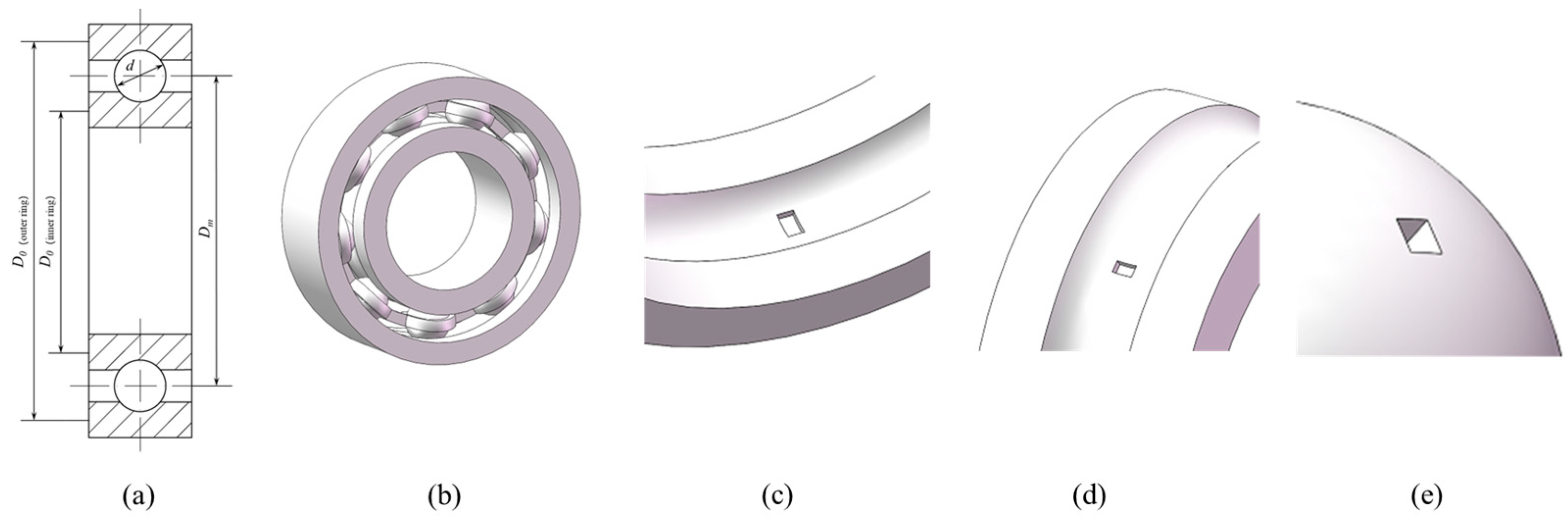
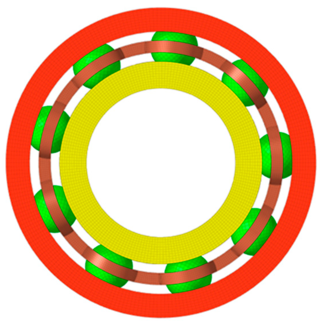
The finite element model was developed to simulate a 6205 deep groove ball bearing with an outer diameter of 52 mm, an inner diameter of 25 mm, a width of 15 mm, and nine rolling elements. The model was constructed in ANSYS/LS-DYNA (2021 R1) through a structured workflow involving geometric modeling, meshing, material property assignment, boundary condition specification, and contact definition. To optimize computational efficiency without compromising accuracy, minor geometric features such as chamfers and rivets were omitted. Defects on the outer race, inner race, and a rolling element were explicitly modeled as rectangular grooves, as illustrated in Figure 1. The mesh consisted of SOLID164 hexahedral elements for the bearing components and SHELL163 shell elements for the raceway surfaces, enabling efficient load application. The final mesh comprised 233,924 elements, ensuring sufficient resolution for precise dynamic analysis (Figure 2).

The material properties were assigned to match real-world bearing components. The inner ring, outer ring, and rolling elements were modeled as GCr15 steel (Elastic Modulus: 206 GPa, Poisson’s Ratio: 0.3), while the cage was simulated using cold-rolled steel (Elastic Modulus: 196 GPa, Poisson’s Ratio: 0.24). In the simulation setup, the outer ring was fully constrained, and the inner ring was subjected to a radial load of 1500 N and a rotational speed of 1797 rpm. To simulate realistic interactions, 27 contact pairs were defined between the rolling elements, raceways, and cage pockets. The inner/outer raceway surfaces and cage pocket surfaces were assigned as target surfaces, while the rolling element outer surfaces were designated as contact surfaces. The static friction coefficients were set to 0.3 (raceways), 0.3 (cage pockets), and 0.002 (rolling elements), with corresponding dynamic friction coefficients of 0.15, 0.15, and 0.001. Acceleration-based vibration data was extracted from a node on the fixed outer ring’s top surface for further analysis.

2.1.3. Model Validation

The reliability of the finite element model is critical, as the similarity between simulated and real-world data determines the feasibility of using transfer learning for fault diagnosis. To systematically validate the model, simulation results were compared against empirical data from the well-established Case Western Reserve University (CWRU) bearing database [46]. While there exists no quantifiable metric to evaluate the similarity between different transfer learning datasets, this study employed a comparative analysis based on domain-specific physical parameters that characterize critical fault features.

Experimental data collected under a 0-horsepower load at a 12 kHz sampling rate served as the benchmark. The analysis focused on three fault types (outer race, inner race, and rolling element), each with three distinct defect diameters (0.1778 mm, 0.3556 mm, and 0.5334 mm). The validation was performed across three domains to ensure a comprehensive assessment: the time domain, by comparing raw signal waveforms; the frequency domain, by analyzing spectra to validate the presence and amplitude of characteristic fault frequencies; and the time-frequency domain, by decomposing the non-stationary signals to compare energy distribution and transient features over time. This systematic validation process confirms the fidelity of the simulation model and establishes the transferability of the generated data for training robust diagnostic models.

2.2. One-Dimensional CNN-Based Fault Diagnosis Model

This study developed a 1D CNN as a foundational model for bearing fault diagnosis. The network was first trained on an extensive simulation-generated dataset to capture fault characteristics under varying conditions. Its generalization capability was then rigorously evaluated using real-world fault data, ensuring robustness across different operational environments. This approach established a pre-trained baseline model optimized for fault identification, providing a reliable foundation for future transfer learning applications in diagnostic systems.

2.2.1. Network Architecture

Given that bearing vibration signals are inherently one-dimensional time-series data, a lightweight 1D CNN was employed to avoid the computational inefficiencies of processing such data with 2D CNNs. The proposed architecture employed a compact design with fewer parameters, enabling effective training with minimal labeled samples. This characteristic is particularly advantageous in industrial scenarios where acquiring large-scale labeled data is often challenging.

The model consists of four convolutional layers, four pooling layers, and two fully connected layers. The input layer processes signal segments of 1024 data points. The feature extraction module begins with a convolutional layer using 32 large kernels (size 32, stride 2) to capture coarse features. Subsequent convolutional layers progressively refine feature extraction with smaller kernels: 64 (size 16), 128 (size 8), and 256 (size 4), all with a stride of 2. Each convolutional layer is followed by a max-pooling layer (size 2, stride 2) to reduce dimensionality and improve feature invariance. This consistent stride of 2 in both convolutional and pooling operations effectively halves the feature map length at each stage, reducing the dimensions from an initial 1024 to 4 × 256 after the final pooling layer.

After feature extraction, the 4 × 256 feature map was flattened into a one-dimensional vector and passed to the classifier, which comprises two fully connected layers with 128 and 10 neurons, respectively. The final layer uses a Softmax activation to output a probability distribution across the 10 fault classes. To enhance training stability and generalization, several regularization techniques were employed. Batch Normalization (BN) was applied after each convolutional and fully connected layer to mitigate internal covariate shift, thereby accelerating convergence and reducing the risk of vanishing gradients. Furthermore, a dropout mechanism was implemented within the fully connected layers to prevent overfitting. A dropout rate of 0.2 was applied after the flattening operation and a rate of 0.5 was applied after the first fully connected hidden layer. The detailed parameters of the network architecture are summarized in

Table 1. Architectural parameters of the 1D CNN model.

Operation	Kernel Size	Stride	Output Channels	Activation Function	Output Size
Convolutional 1	32	2	32	ReLU (+BN)	512 × 32
Max Pooling 1	2	2	32	/	256 × 32
Convolutional 2	16	2	64	ReLU (+BN)	128 × 64
Max Pooling 2	2	2	64	/	64 × 64
Convolutional 3	8	2	128	ReLU (+BN)	32 × 128
Max Pooling 3	2	2	128	/	16 × 128
Convolutional 4	4	2	256	ReLU (+BN)	8 × 256
Max Pooling 4	2	2	256	/	4 × 256
Flatten	/	/	/	/	1024
Dropout (0.2)	/	/	/	/	1024
Fully Connected1	/	/	/	ReLU (+BN)	128
Dropout (0.5)	/	/	/	/	128
Fully Connected2	/	/	/	Softmax	10

Note: ‘/’ indicates that the parameter is not applicable to this operation.

.

2.2.2. Training Configuration

The model was trained on bearing simulation data generated through finite element analysis. The dataset includes 10 operational conditions: Normal (N), Inner Race Fault (IR), Ball Fault (B), and Outer Race Fault (OR), each with three defect diameters (0.1778 mm, 0.3556 mm, and 0.5334 mm). For each condition, 1000 signal segments (1024 data points each) were randomly sampled. The dataset was split into a 90% training set for model optimization and a 10% testing set for final evaluation. Training was performed using the Adam optimizer, which adapts learning rates based on first and second-order gradient moments to efficiently optimize the network. A fixed initial learning rate of 0.001 was applied, with exponential decay to ensure stable convergence. Due to the lightweight architecture of the 1D CNN, training completed in just 50 epochs, which was sufficient to achieve optimal performance without overfitting.

2.3. A Deep Domain Adaptation Framework Using GAN and MK-MMD

Deep neural networks trained solely on simulated data exhibit substantially reduced classification accuracy in real-world fault diagnosis applications. While bearing simulations preserve characteristic fault signatures, inherent distributional discrepancies between simulated and actual operational data persist. To address this issue, this section proposes a deep domain adaptation transfer learning method that combines Generative Adversarial Networks (GANs) with Multi-Kernel Maximum Mean Discrepancy (MK-MMD) to overcome the domain shift and improve the model’s generalization capability.

2.3.1. Principles of Multi-Kernel Maximum Mean Discrepancy (MK-MMD)

Maximum Mean Discrepancy (MMD) is a statistical metric designed to quantify the dissimilarity between two probability distributions. The fundamental concept involves mapping samples from a source domain (X) and a target domain (Y) into a high-dimensional Reproducing Kernel Hilbert Space (RKHS) [47], where the distance between the means of the two mapped distributions can be calculated. The squared MMD is formally expressed as:

$$MM{D}^2(X,Y)={‖{\displaystyle \frac{1}{n}}{\displaystyle \sum _{i=1}^n\varphi \left(x_i\right)-\frac{1}{m}{\displaystyle \sum _{j=1}^m\varphi \left(y_j\right)}}‖}_H^2$$

(6)

where x_i and y_j are samples from the source and target domains, respectively; n and m are the corresponding sample sizes; and ϕ is the mapping function to the RKHS. By applying the kernel trick, where K(x,y) = φ(x)φ(y), the computationally intensive inner product in the RKHS can be avoided. This transforms the MMD expression into

$$MM{D}^2(X,Y)=\frac{1}{n^2}\sum _i^n\sum _i^{n}K\left(x_i,x_i\right)-\frac{2}{nm}\sum _i^n\sum _j^{m}K\left(x_i,y_j\right)+\frac{1}{m^2}\sum _j^m\sum _j^{m}K\left(y_j,y_j\right)$$

(7)

The choice of kernel function significantly influences the performance of MMD. To enhance the model’s representational capacity and avoid suboptimal kernel parameter selection, a multi-kernel MMD (MK-MMD) approach was employed. This method utilizes a linear combination of multiple kernels, typically Gaussian kernels with varying bandwidths (σ), to better capture the distribution discrepancies at different scales. The multi-kernel function is defined as

$$K\triangleq \{k=\sum _{u=1}^m{\beta }_u{k}_u:\sum _{u=1}^m{\beta }_u=1,{\beta }_u\ge 0,\forall u\}$$

(8)

where k_u represents a distinct kernel (e.g., a Gaussian kernel $K\left(x,y\right)=e^{{\displaystyle \frac{-\Vert x-y{\Vert }^2}{2{\sigma }^2}}}$ with a specific bandwidth) and β_u are the corresponding weighting coefficients.

2.3.2. Principles of Generative Adversarial Networks (GANs)

Proposed by Goodfellow et al. in 2014 [37], the Generative Adversarial Network (GAN) was inspired by two-player game theory. A GAN comprises two neural networks: a Generator (G) and a Discriminator (D), which are trained in an adversarial manner. The Generator takes random noise or source domain data as input and attempts to generate synthetic samples that are indistinguishable from real data. The Discriminator’s objective is to accurately differentiate between real samples from the target domain and the synthetic samples produced by the Generator. This competitive process iteratively refines both networks. The optimization objective of a standard GAN is represented by the following min–max game:

$${\min }_G\left\{\underset{D}{\max }V(D,G)\right\}=E_{P_r}(x)(\log D(x))+E_{P_z}(z)[\log (1-D(G(z)))]$$

(9)

where P_r and P_z are the data distributions of the target domain and the source domain input to the generator, and V is the value function of the discriminator. The optimization process of GANs involves two competing objective function. The max function represents the discriminator’s optimization goal, while the min function corresponds to that of the generator. This alternating optimization between the two functions reflects the adversarial training dynamic, where the generator and discriminator continuously improve through mutual competition.

The training procedure consists of two distinct phases. In the Discriminator Training phase, the generator’s parameters are held fixed while the discriminator is optimized to maximize its value function V. The discriminator’s role is to differentiate between real samples and those produced by the generator, effectively treating this as a binary classification task. Its output, generated using the Sigmoid function, produces values in the range [0, 1]. To maximize V, it is necessary to drive the discriminator’s output D(x) for real samples x toward 1, while pushing the output D(G(z)) for generated samples G(z) toward 0. When optimally trained, the discriminator becomes highly accurate, correctly classifying real samples as 1 and generated samples as 0. In the Generator Training phase, the discriminator’s parameters are fixed, and the generator is trained to minimize its value function V. Here, the generator adjusts its parameters to increase the discriminator’s output D(G(z)), pushing it toward 1, which means the generated samples become indistinguishable from real data. Through this iterative process, the generator and discriminator engage in continuous adversarial refinement, ultimately enabling the generator’s output distribution to approximate the real data distribution, thereby achieving high-quality generation results.

2.3.3. The Proposed Deep Domain Adaptation Model

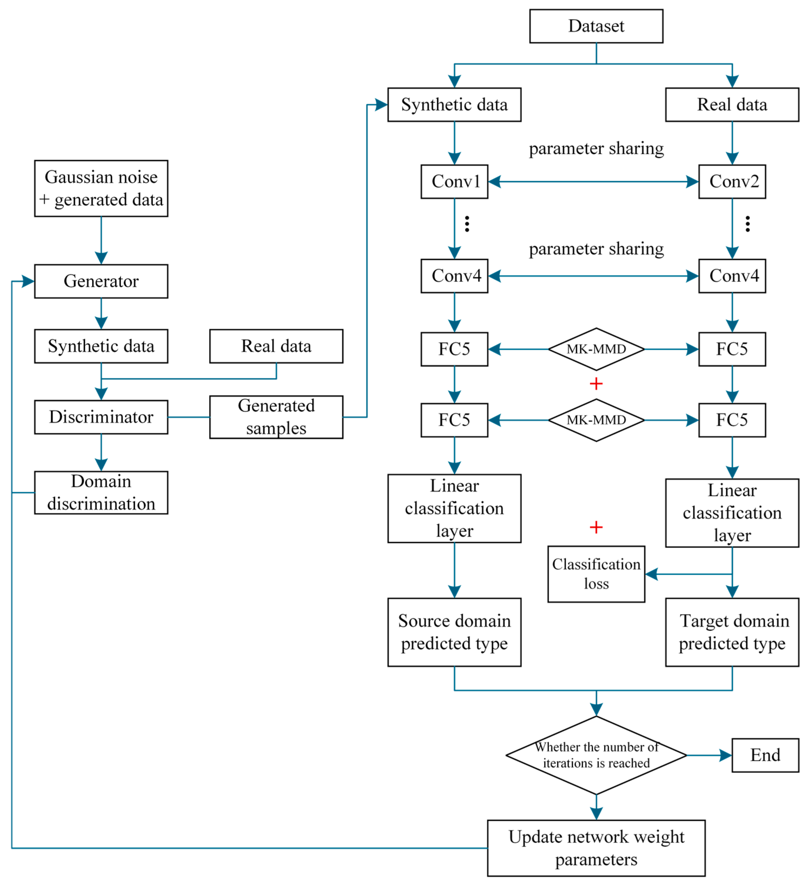
To bridge the domain gap between simulated and actual fault data, a deep domain adaptation model that integrates a GAN with the MK-MMD metric was proposed. The architecture, depicted in Figure 3, consists of three core components: a generator, a discriminator, and a classifier.

The generator takes Gaussian noise and labeled simulated data as inputs to produce synthetic data whose distribution mimics that of the real-world data. The discriminator is trained to distinguish between these generated samples and unlabeled real data, compelling the generator to create more realistic outputs. The classifier, which is the 1D CNN model established in Section 2.2, acts as a deep feature extractor. It is trained on the labeled generated data and subsequently tested on real data to predict the bearing’s health status.

To enhance training efficiency and leverage shared knowledge, the shallow convolutional layers of the classifier, which learn general fault features, are shared between the source and target domains. In contrast, the deeper, fully connected layers learn more domain-specific diagnostic knowledge. The discrepancy between the feature distributions learned by these higher-level layers for the two domains is quantified using the MK-MMD metric. This metric is incorporated into the loss function to explicitly minimize the domain shift.

The model training involves optimizing three interconnected objective functions. The discriminator’s objective is to maximize

$$L_D=E_{P_r}(x)(\log D(x))+E_{P_z}(z)\left[\log \left(1-D\left(G(z)\right)\right)\right]$$

(10)

The generator’s objective is to minimize

$$L_{\mathrm{G}}=E_{P_z}(z)\left[\log \left(1-D\left(G(z)\right)\right)\right]$$

(11)

Simultaneously, the optimization goal for the feature extractor and classifier involves minimizing both the classification cross-entropy loss (J) and the MK-MMD distance between the generated and real feature distributions (L_MK-MMD (D_s, D_t)):

$$L_C=J+L_{MK\text{-}MMD}(D_s,D_t)$$

(12)

The final integrated objective function for optimization is

$$L=L_C+{\lambda }_1{L}_G+{\lambda }_2{L}_D$$

(13)

where λ₁ and λ₂ denote weighting coefficients that balance the contributions of the adversarial loss and the domain discrepancy loss.

2.3.4. Model Dataset Configuration and Network Architecture

The dataset was structured with a training set comprising both source domain (simulated) and target domain (real-world) data, while the test set consisted solely of real-world data. The data was classified into 10 distinct categories: one normal condition and three fault types (outer race, inner race, and rolling element), each with three levels of severity. A sliding window of 1024 data points was used to segment the time-series signals into samples. The training set includes 1000 samples per class, and the test set includes 100 samples per class.

The generator architecture consists of five 1D convolutional layers. The first four layers utilize ReLU activation, while the final layer employs a Tanh activation function to accommodate the negative values inherent in vibration signals. The discriminator is composed of five 1D convolutional layers with ReLU activation. The output of the final convolutional layer is flattened and passed to a fully connected layer with a Sigmoid function to output a probability. The classifier employs the 1D CNN architecture previously designed. Specific structural details of the generator and discriminator are provided in

Table 2. Structural details of the generator and discriminator networks.

Component	Operation	Kernel Size	Stride	Activation Function	Channels
Generator Network	Conv1	32 × 1	1	ReLU	8
	Conv2	32 × 1	1	ReLU	16
	Conv3	32 × 1	1	ReLU	8
	Conv4	32 × 1	1	ReLU	2
	Conv5	32 × 1	1	Tanh	1
Discriminator Network	Conv1	32 × 1	2	ReLU	96
	Conv2	16 × 1	2	ReLU	64
	Conv3	8 × 1	1	ReLU	32
	Conv4	5 × 1	1	ReLU	16
	Conv5	3 × 1	1	ReLU	32
	Flatten	/	/	/	/
	Fully Connected	/	/	Sigmoid	1

Note: ‘/’ indicates that the parameter is not applicable to this operation.

.

3. Results and Discussion

3.1. Validation of the Finite Element Simulation Model

To evaluate the fidelity of the developed FE model, a multi-faceted validation was conducted by comparing simulation results with experimental data across the time, frequency, and time-frequency domains. This comprehensive approach ensures that the model accurately captures the dynamic characteristics of bearing faults under various conditions.

3.1.1. Time-Domain Statistical Validation

Time-domain statistical indicators, such as impulse factor, margin index, and kurtosis, are widely used in signal analysis and fault diagnosis due to their proven diagnostic effectiveness. Vibration signals from both simulations and experiments, corresponding to bearing defect sizes of 0.1778 mm and 0.5334 mm, were first normalized. From each dataset, ten 1200-point segments were randomly selected, and the average values of the statistical indicators were calculated. The results, summarized in

Table 3. Time-domain statistical indicators of actual data versus simulated data.

Bearing Health Condition	Impulse Indicator		Margin Indicator		Kurtosis Indicator
	Actual	Simulated	Actual	Simulated	Actual	Simulated
Healthy Bearing	4.166	4.231	4.910	4.993	2.868	2.908
Rolling Element Fault (0.1778)	4.664	4.545	5.481	5.359	2.950	2.956
Rolling Element Fault (0.5334)	4.727	4.856	5.592	5.740	7.666	7.624
Inner Race Fault (0.1778)	5.213	5.273	6.162	6.233	5.528	5.511
Inner Race Fault (0.5334)	6.572	6.697	7.746	7.922	7.072	7.026
Outer Race Fault (0.1778)	7.722	7.52	10.463	10.069	7.666	7.624
Outer Race Fault (0.5334)	12.599	12.483	15.079	15.083	22.053	21.530

, show strong agreement between simulation and experimental data, with relative deviations below 3% for all indicators. Notably, kurtosis, the most sensitive parameter to impulsive events, exhibited a maximum deviation of only 2.5%. These minor discrepancies confirm the high reliability of the simulation model in the time-domain statistical analysis. Moreover, the results consistently reveal a positive correlation between defect size and the magnitude of the indicators, where larger faults yield correspondingly higher values, a trend accurately captured by the model.

3.1.2. Frequency-Domain Envelope Spectrum Validation

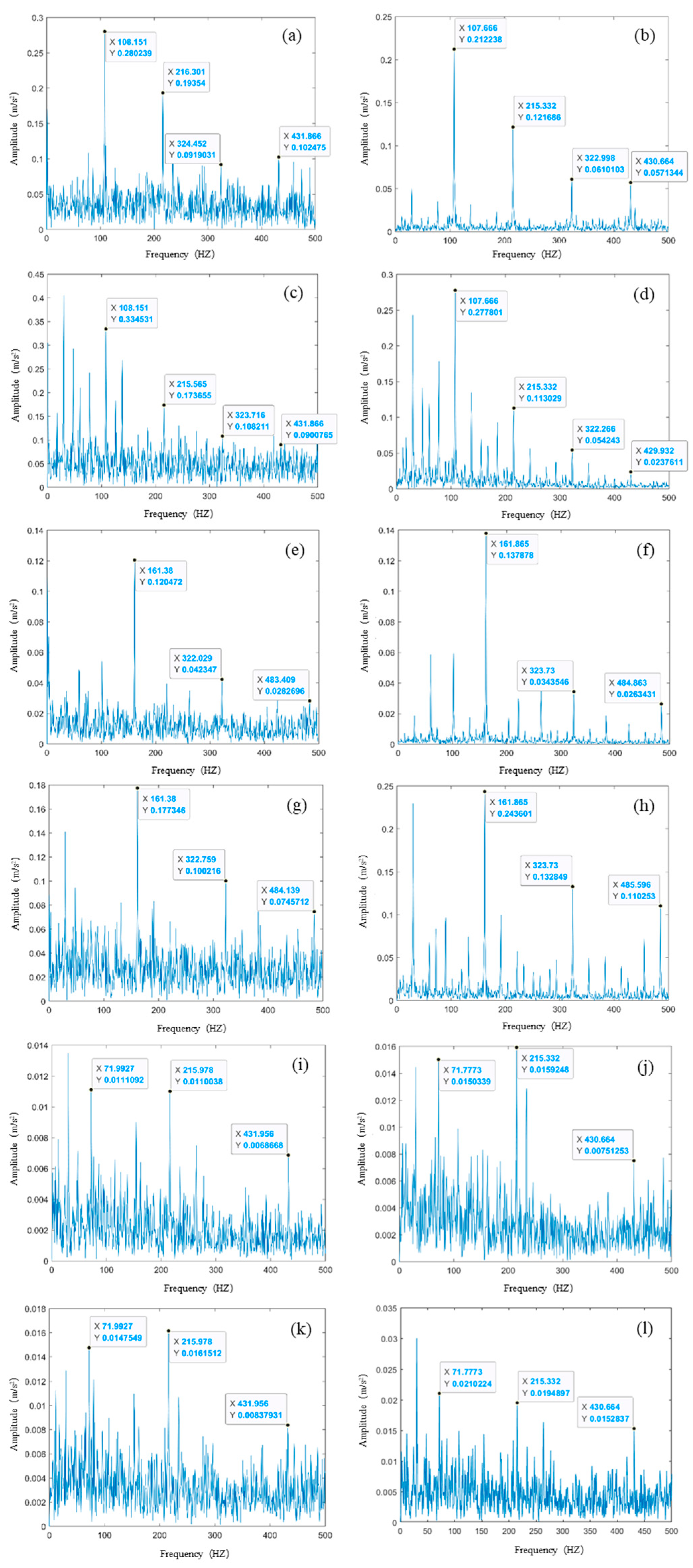
After the time-domain analysis, the model’s accuracy was further evaluated in the frequency domain using envelope spectrum analysis, a technique highly effective for identifying periodic impacts characteristic of bearing faults. Based on the bearing parameters and an operational speed of 1797 r/min, the theoretical characteristic fault frequencies were calculated as 107.36 Hz for an outer race fault (f_o), 162.19 Hz for an inner race fault (f_i), and 70.58 Hz for a rolling element fault (f_b).

As shown in Figure 4a–d, the dominant frequencies in the simulated (108.151 Hz) and experimental (107.666 Hz) spectra align closely with the theoretical outer race fault frequency, exhibiting minimal deviations of 0.74% and 0.28%, respectively. The spectra for inner race faults, shown in Figure 4e–h, exhibit greater complexity. This is attributable to the modulation of the fault frequency by the shaft’s rotational frequency, which produces distinct sidebands. Despite this complexity, the primary simulated (161.38 Hz) and experimental (161.865 Hz) fault frequencies show excellent agreement with the theoretical value, with deviations of only 0.50% and 0.20%. The rolling element fault spectra shown in Figure 4i–l are the most intricate, a consequence of the complex kinematics of the rolling elements. While the frequency deviations were slightly larger (2% for simulation and 1.7% for experimental), they remain well within acceptable limits. A crucial observation across all fault conditions is that the defect severity primarily influences the amplitude of the spectral peaks rather than their frequency location. This confirms that the model accurately captures the physical principle that fault magnitude governs vibration intensity rather than altering the fundamental spectral structure.

3.1.3. Time-Frequency Domain Validation

For a comprehensive time-frequency analysis, a feature extraction method combining Empirical Mode Decomposition (EMD) [48] and Singular Value Decomposition (SVD) [49] was employed. The rationale for this approach is the inherent stability of singular values. As intrinsic characteristics of a matrix, they exhibit robustness to minor perturbations in the signal data and thus serve as reliable fault feature vectors. The methodology involves first decomposing the vibration signal into a set of Intrinsic Mode Functions (IMFs). These IMFs are then used to construct a feature matrix, to which SVD is applied. The resulting singular values represent the signal’s energy distribution across different frequency bands.

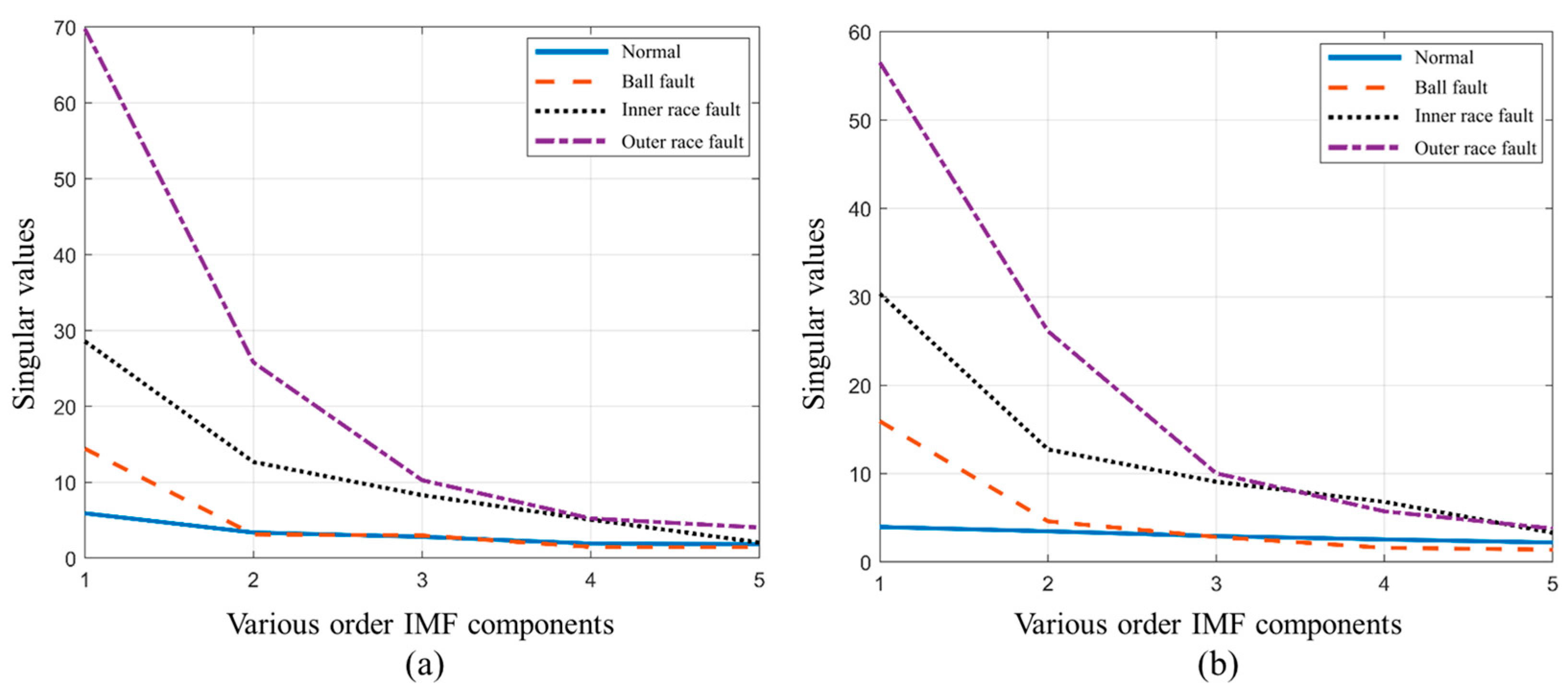
Figure 5 illustrates the trends of the first five singular values for both experimental and simulated signals, while

Table 4. Singular value entropy of actual signals and simulated model signals.

Bearing Condition	Actual Signal	Simulated Signal
Normal	1.8392	1.7553
Ball Fault	1.4957	1.521
Inner Race Fault	1.7264	1.7112
Outer Race Fault	1.5172	1.5602

presents the corresponding singular value entropy. A strong consistency is observed in the trends for both the singular values and the entropy across different bearing health states. Specifically, for all fault conditions, the first five singular values are markedly greater than those of a healthy bearing, whereas the singular value entropy is lower. This phenomenon is attributed to the concentration of vibration energy within specific fault-related frequency bands, which reduces the overall uncertainty and consequently the entropy of the signal’s energy distribution. These results demonstrate that the established simulation model accurately reflects the fault characteristics of bearings.

3.2. Baseline Model: Direct Transfer Without Domain Adaptation

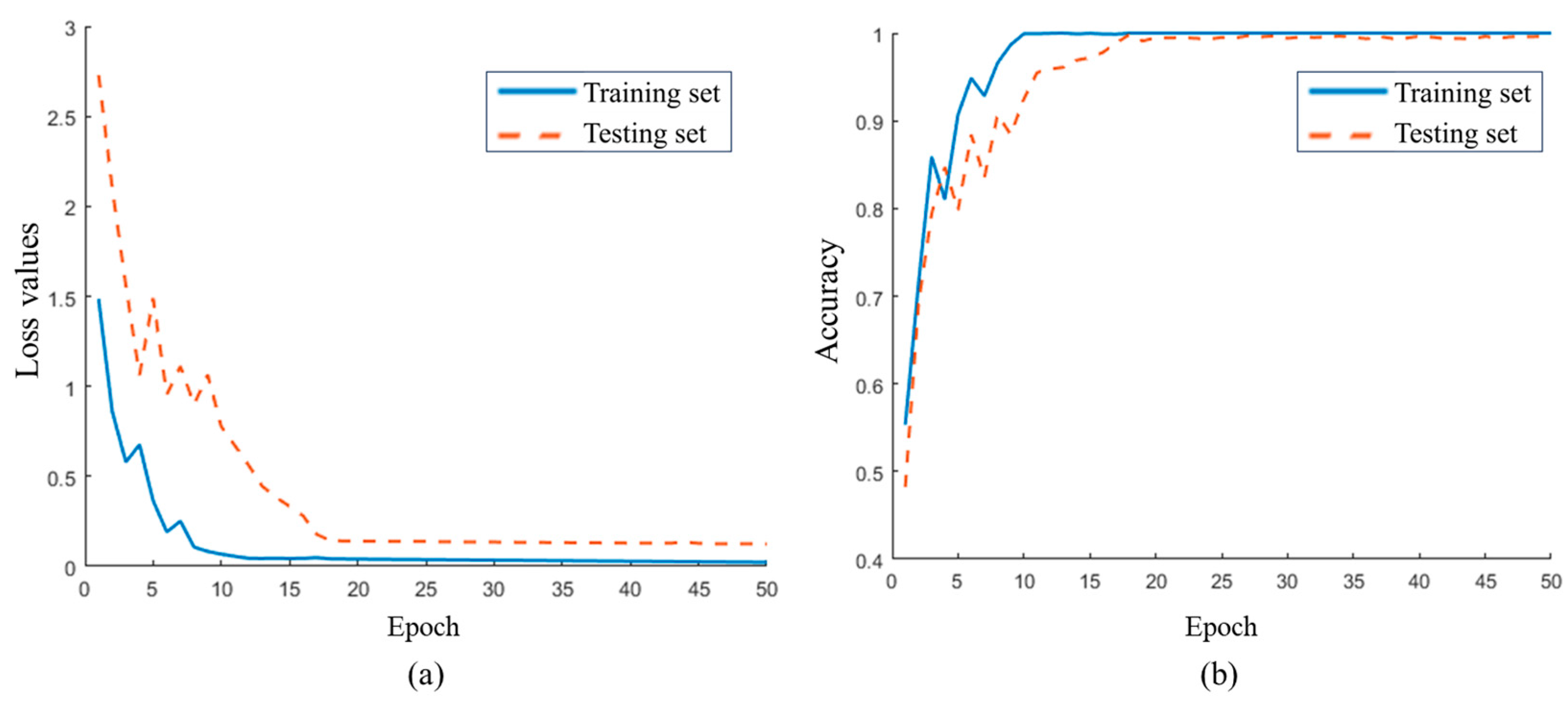
To establish a performance baseline and demonstrate the necessity of domain adaptation, a standard 1D CNN was initially evaluated. The model was first trained on the simulated dataset, where it exhibited strong convergence, as evidenced by the loss and accuracy curves in Figure 6. In Figure 6a, the loss value on the training set decreases continuously, dropping to a very low level after several epochs and approaching zero by the 10th epoch. On the test set, the loss also shows an overall downward trend, albeit with minor fluctuations in the first 10 epochs before stabilizing around 0.1. Similarly, the accuracy curve in Figure 6b reveals an inverse relationship with the loss, increasing as the loss declines. After some initial fluctuations in the first 15 epochs, the accuracy stabilizes, reaching 100% on the training set and 99.5% on the test set. These results confirm that the network parameters were effectively optimized for the source (simulation) domain.

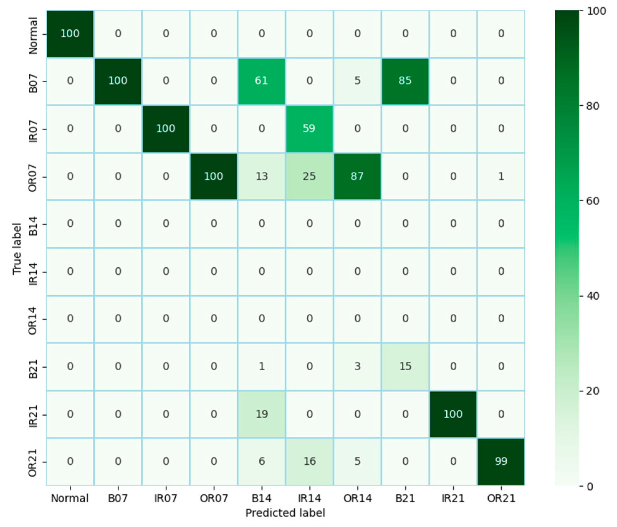
However, when this pre-trained model was directly applied to the target domain (experimental CWRU data) for fault diagnosis, its performance deteriorated significantly. The test set consisted of real-world data from the CWRU bearing dataset, encompassing 10 categories of bearing health conditions, with 100 samples per category and a signal length of 1024 for each sample. As shown in the confusion matrix (Figure 7), “normal” represents the healthy state, while B07, B14, and B21 denote rolling element faults of varying severities (0.007, 0.014, and 0.021 inches, respectively). Similarly, IR07, IR14, and IR21 indicate inner race faults, and OR07, OR14, and OR21 represent outer race faults. Despite identifying some patterns, the model achieved only 61.4% overall accuracy. Theoretically, a randomly initialized model would yield around 10% accuracy for a 10-class classification task. While the proposed model significantly outperforms this baseline, demonstrating that it has learned meaningful fault features from the training data, its performance remains limited due to domain discrepancies between the simulated training set and the real-world test data. This substantial drop in accuracy clearly reflects the inherent challenges of cross-domain fault diagnosis and highlights the need for transfer learning to bridge the gap between simulation and real-world applications. Thus, further refinement through domain adaptation is essential to improve the model’s diagnostic accuracy on experimental bearing data.

3.3. Proposed Model: Deep Domain Adaptation from Simulation to Reality

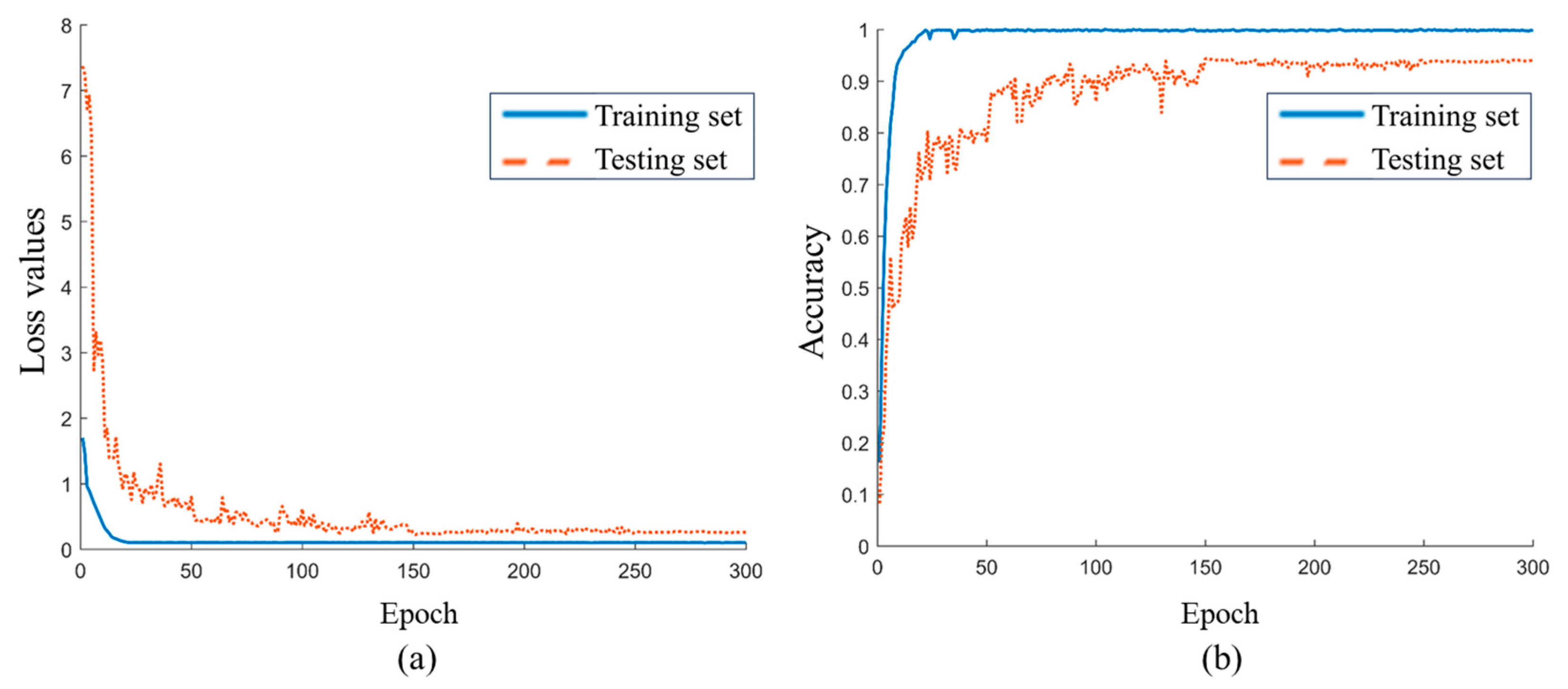
To address the domain shift problem, the proposed deep domain adaptation model was implemented and evaluated on the same simulation-to-real transfer task. As shown in Figure 8a, the model achieves 100% training accuracy by the 30th epoch, while on the test set, accuracy exceeds 93% by the 150th epoch and stabilizes between 93% and 94%. The final 30-iteration average test accuracy is 93.8%. Figure 8b illustrates the convergence of training and test loss values around the 30th and 150th epochs, respectively, reaching approximately 0.1 (training) and 0.25 (test). The higher test loss is expected, as the training set benefits from supervised learning, whereas the test set relies on transferred knowledge, leading to marginally weaker classification performance. To benchmark our approach against established methods, we compared it with the developed 1D CNN, DAN, and DANN. To ensure a fair evaluation, all comparative models utilized the same 1D CNN feature extraction backbone as detailed in Table 1 (Section 2.2.1). For DAN and DANN, the specific domain adaptation modules and loss functions were implemented strictly following the guidelines provided in their original studies [34,35] and [32,33], respectively. Both baseline models were trained in an end-to-end manner using the Adam optimizer with standard momentum settings. Additionally, for the DANN model, the domain adaptation parameter was dynamically adjusted following the standard schedule described in [32,33].

While accuracy serves as the primary metric for monitoring training progress and overall trends, a more comprehensive evaluation is necessary to assess the model’s robustness across specific fault classes. Therefore, the Precision, Recall, and F1 scores based on the confusion matrices were further calculated. As shown in

Table 5. Summary of predictive performance metrics among models.

Model	1D CNN	DAN	DANN	Proposed Model
Accuracy (%)	61.40	88.30	91.40	93.80
Precision (%)	48.84	87.59	91.70	94.93
Recall (%)	61.40	88.30	91.40	93.80
F1-Score (%)	49.95	86.85	91.37	93.37

, the 1D CNN performs poorly under domain discrepancy, achieving only 61.40% accuracy. More critically, its F1-score drops to 49.95%, and its precision is just 48.84%. This significant disparity suggests that the 1D CNN is biased toward certain classes while failing to generalize to others, leading to a high false-positive rate. In contrast, the domain adaptation baselines, DAN and DANN, show marked improvements. DAN achieves an F1-score of 86.85%, while DANN reaches 91.37%, reflecting more balanced classification performance. However, the proposed model outperforms all baselines, attaining the highest accuracy (93.80%) and F1-score (93.37%). Notably, it achieves a precision of 94.93%, significantly surpassing both DAN (87.59%) and DANN (91.70%). This high precision confirms that the proposed framework is not only accurate but also robust against false alarms.

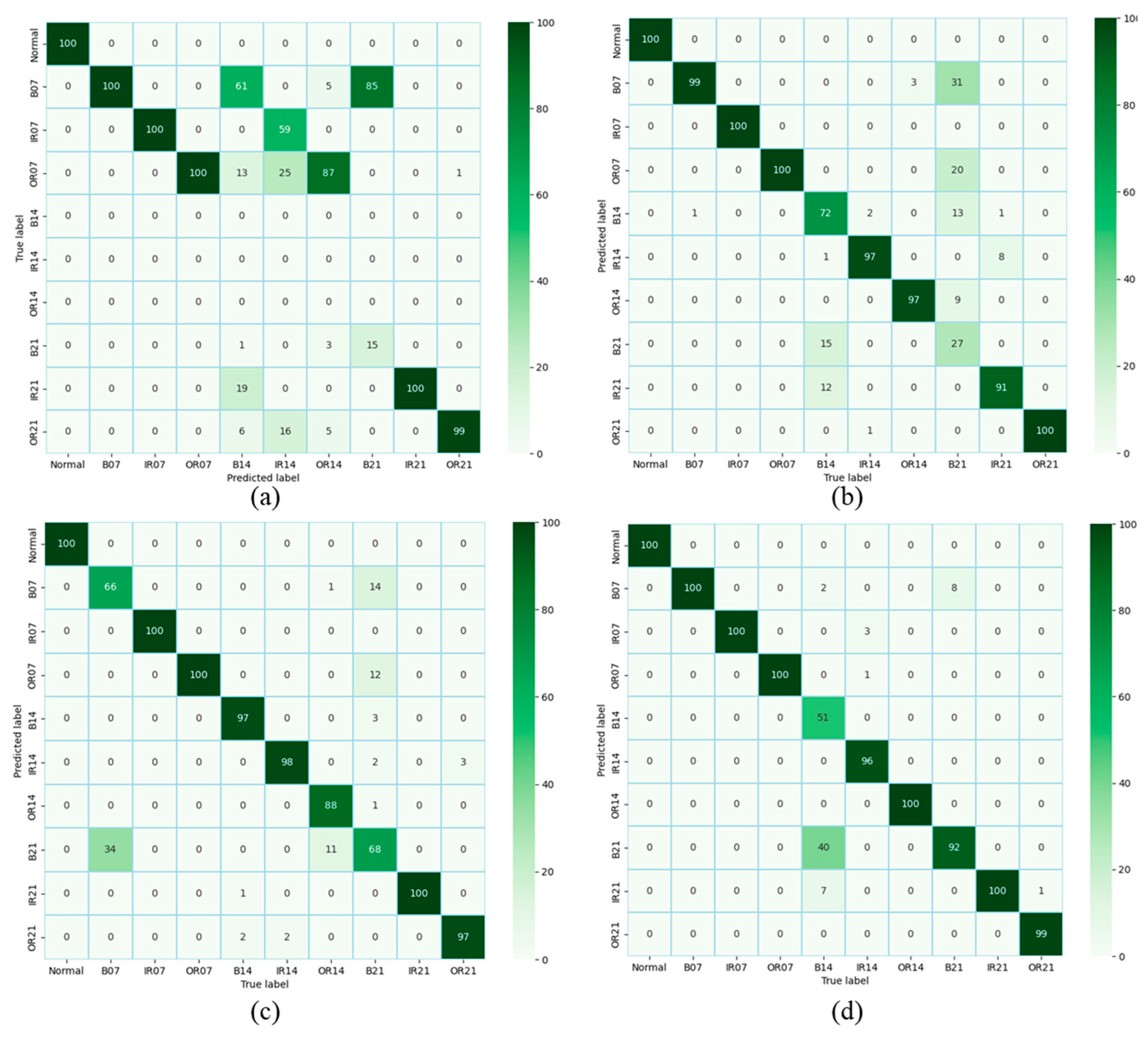
A deeper analysis of the confusion matrices in Figure 9 explains the source of the observed improvement. The results show that the three domain adaptation models outperform the 1D CNN baseline in both accuracy and recall rates across most categories, with the most notable enhancements in classifying B14, IR14, OR14, and B21. For a more detailed comparison between the proposed method and DAN/DANN, classifications are categorized as coarse and fine categories. Coarse classification is based on bearing health status, including normal conditions, inner race faults, outer race faults, and rolling element faults, while fine classification refers to different fault sizes within the same fault type, categorized as 07, 14, and 21. The confusion matrices reveal that DAN misclassifies 49 samples in coarse classification, while DANN reduces this to 35 misclassifications. In contrast, the proposed model achieves significantly better performance, misclassifying only 9 samples. All three models exhibit errors in fine classification, primarily in distinguishing rolling element fault sizes. However, the proposed model consistently surpasses DAN and DANN, demonstrating superior diagnostic capability for bearing faults.

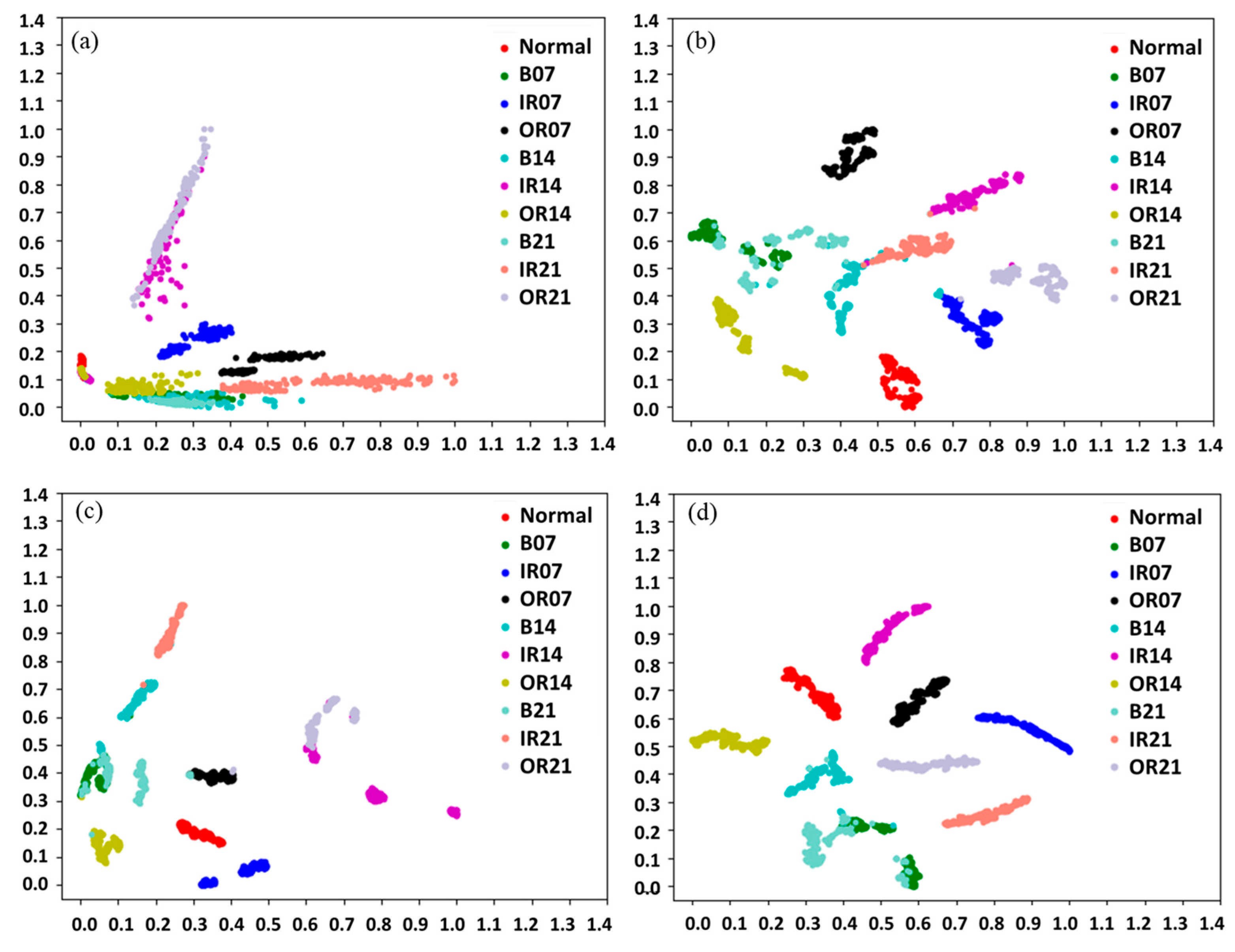
A t-SNE visual analysis was conducted to compare the feature distributions of the four models, as illustrated in Figure 10. The 1D CNN model shows poorly defined clusters, with fault categories heavily intermixed and no discernible boundaries. While the DAN exhibits improved classification performance compared to 1D CNN, with distinct boundaries between most fault categories, though significant overlap persists for B07 and B14. The DANN model further reduces overlapping compared to DAN but shows poorer aggregation of target features within the same category. In contrast, the proposed model achieves superior classification performance, with the 10 fault categories largely separated and minimal large-scale overlap. Although some overlap remains for B07, B14, and B21, the boundaries between different categories are more distinct. These results highlight the proposed model’s enhanced ability to generalize in the target domain, achieving both stronger inter-class separation and intra-class compactness.

3.4. Robustness Evaluation on Real-World Datasets

To further assess the model’s generalization capabilities and robustness, its performance was evaluated on more challenging transfer tasks using exclusively experimental data from the CWRU and Jiangnan University (JNU) databases [50].

3.4.1. Robustness to Varying Operating Conditions

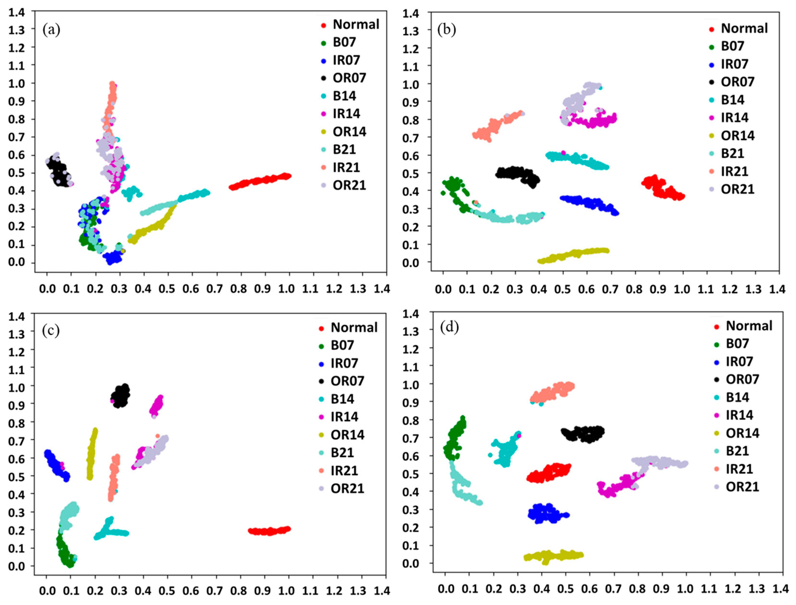
The model’s adaptability to varying operating conditions was evaluated using datasets from the CWRU database, recorded at different rotational speeds (

Table 6. Dataset configurations under different rotational speeds.

Dataset	A	B	C	D
Rotational Speed (r/min)	1790	1772	1750	1730

). Each dataset consists of 10 classes, with 1000 samples per class. The training and test sets were split in a 9:1 ratio, resulting in 900 and 100 samples, respectively. For transfer learning tasks across datasets with differing rotational speeds, the proposed model was benchmarked against 1D CNN, DAN, and DANN models. As shown in

Table 7. Fault diagnosis accuracy (%) under varying operating conditions.

Transfer Task	1D CNN	DAN	DANN	Proposed Method
A → B	85.9	97.2	98.3	99.2
A → C	73.3	92.3	93.4	96.8
A → D	59.1	86.9	88.8	91.1
B → C	84.5	97.8	98.6	99.3
B → D	75.6	92.2	92.9	97.1
C → D	84.9	97.1	97.9	99.3
Average Accuracy	77.22	93.91	94.98	97.1

, the proposed model consistently outperformed all baselines across six transfer tasks, achieving an average accuracy of 97.1%. This represents a significant improvement of 3.19% over DAN and 2.12% over DANN. Notably, even in the most challenging task with the largest speed discrepancy (A → D), the proposed model maintained an accuracy of 91.1%. The corresponding t-SNE visualizations in Figure 11 further confirm the proposed model’s superior ability to learn domain-invariant features, resulting in better clustering. A comparative analysis of Figure 10 and Figure 11, and Table 5, Table 6 and Table 7 demonstrates that transfer learning using simulated data yields better classification performance than methods relying on data from disparate operating conditions. This advantage becomes particularly pronounced when operating conditions exhibit significant discrepancies.

3.4.2. Robustness to Different Bearing Types

To evaluate the accuracy of the proposed model when applied to vibration signals from different bearings, datasets from the CWRU bearing database and the Jiangnan University (JNU) centrifugal fan rolling bearing fault diagnosis testbed were employed. The CWRU dataset includes vibration signals collected from drive-end SKF6205 and fan-end SKF6203 bearings, sampled at 12 kHz under rotational speeds of 1730 rpm and 1797 rpm, respectively. In contrast, the JNU dataset consists of single-row spherical roller bearings sampled at 50 kHz under a rotational speed of 1000 rpm. Due to differences in fault severity across the datasets, the experiment focused solely on classifying four health states rather than fault severity. The bearing configurations, including variations in bearing type, roller count, and sampling rate, are detailed in

Table 8. Parameters of bearing datasets.

	Dataset	Bearing Model	Bearing Type	Sampling Frequency	Roller Count	Rotational Speed
A	CWRU	SKF 6205	Deep Groove Ball Bearing	12 kHz	9	1797 rpm
B		SKF 6205	Deep Groove Ball Bearing	12 kHz	8	1730 rpm
C		SKF 6203	Deep Groove Ball Bearing	12 kHz	8	1797 rpm
D	JNU	N/A	Single-Row Spherical Roller Bearing	50 kHz	13	1000 rpm

. Each class contains 1000 samples to ensure consistent evaluation.

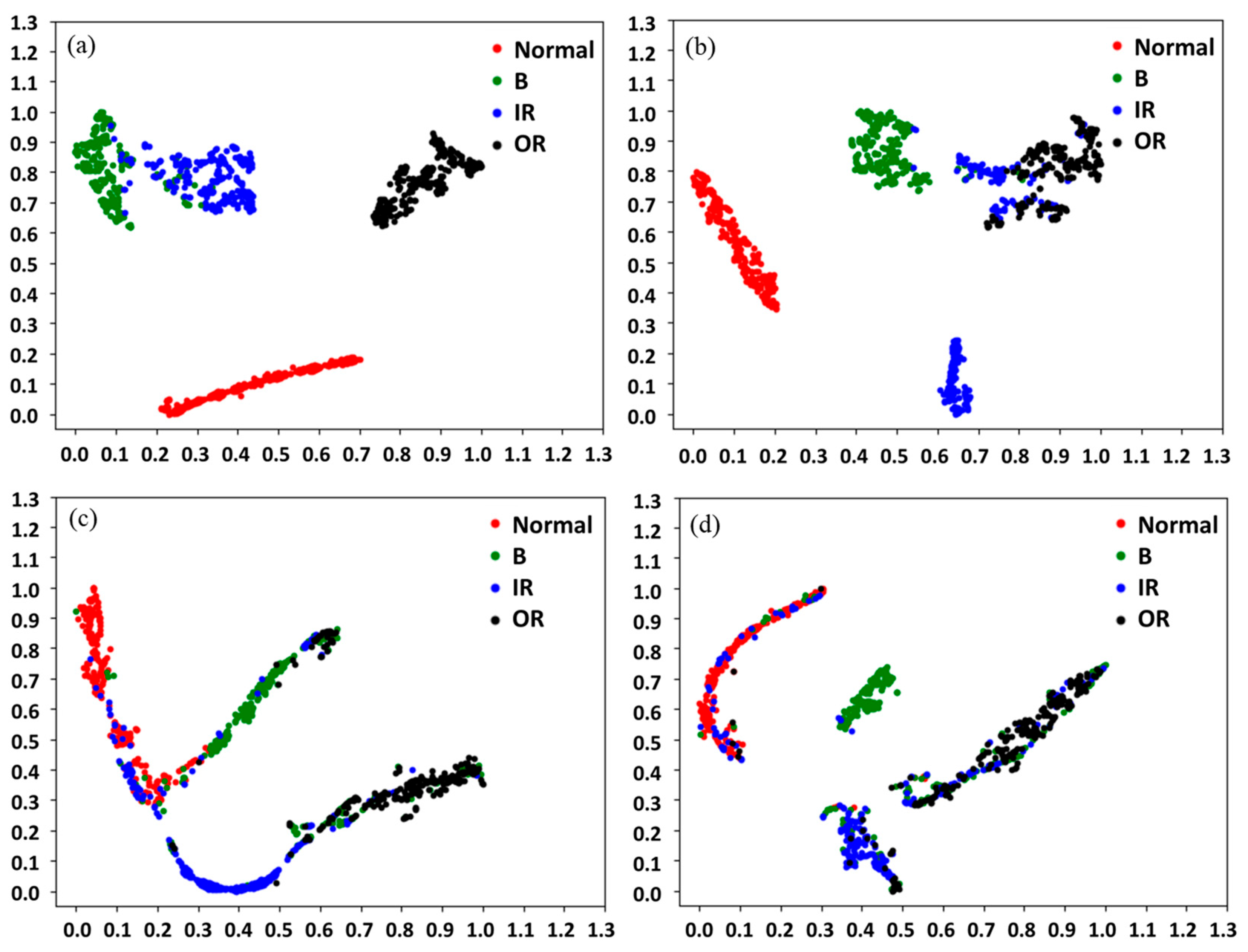
The proposed model was compared with 1D CNN, DAN, and DANN models for cross-dataset transfer learning. The results (

Table 9. Fault diagnosis accuracy (%) for cross-dataset tasks.

Transfer Task	1D CNN	DAN	DANN	Proposed Method
A → C	47.1	73.1	72.5	75.5
B → C	43.7	61.5	62.7	68.5
A → D	29.7	45.2	46.5	47.7
C → D	30.2	45.7	45.3	47.2
Average Accuracy	37.675	56.375	56.75	59.725

) and visualization analysis (Figure 12) reveal that the accuracy of tasks A → D and C → D is significantly lower than that of tasks A → C and B → C. This discrepancy arises because datasets A, B, and C are derived from the CWRU database, sharing the same sampling frequency and bearing type (deep groove ball bearings), whereas dataset D from JNU differs in bearing type, sampling frequency, and rotational speed. These findings highlight those variations in bearing type, sampling frequency, and rotational speed negatively impact classification accuracy, with larger discrepancies leading to more pronounced performance degradation.

3.4.3. Generalization Analysis and Practical Implications

The significant domain shift observed (accuracy drop to 61.4%) is physically attributed to the complexity of the real-world transmission path and environmental noise, which masks the clear fault signatures present in the FE simulation. From an engineering perspective, the rationale for employing the proposed MK-MMD domain adaptation is its ability to extract domain-invariant features. Since the fundamental mechanics of the bearing fault remain consistent between the physics-based simulation and the physical experiment, the domain adaptation layer functions as a non-linear filter. It aligns the feature distributions by suppressing the discrepancies caused by the variable transmission paths and noise floors, thereby isolating the consistent physical fault signatures common to both domains.

Regarding the generalization capability, the dual-dataset validation (CWRU and JNU) presented in the preceding sections confirms that the model’s robustness extends beyond a single experimental setup. This validation strategy aligns with recent protocols established in independent studies [51], demonstrating that the extracted features capture intrinsic fault mechanisms rather than dataset-specific artifacts. A critical insight emerging from this evaluation is that transfer learning performance is inversely proportional to the magnitude of the physical domain shift. While the model shows robustness to moderate variations in operating conditions (Section 3.4.1), large discrepancies, particularly the transition from deep groove ball bearings (CWRU) to single-row spherical roller bearings (JNU) combined with a drastic shift in sampling rate (12 kHz vs. 50 kHz), result in a notable decline in accuracy (Section 3.4.2). Crucially, however, the initial simulation-to-real transfer task achieved a higher accuracy (93.8%) than these challenging cross-database real-to-real tasks. This finding aligns with the simulation-driven philosophy discussed by Liu et al. [52], who demonstrated that physics-based simulation data can effectively bridge the domain gap when real-world fault data is scarce. Consequently, this study strongly supports the hypothesis that a strategy combining high-fidelity FE simulation with advanced deep domain adaptation offers a practical, scalable, and effective pathway. It addresses the limitation of data scarcity in industrial scenarios, providing a reliable foundation for developing intelligent fault diagnosis systems for real-world engineering applications.

4. Conclusions and Future Work

This study addressed the persistent challenge of insufficient training data for deep learning-based bearing fault diagnosis by proposing and validating a novel methodology that integrates high-fidelity finite element simulation with advanced transfer learning. The results demonstrate that a rigorously validated simulation model can effectively serve as a reliable training data source, bridging the gap between theoretical models and real-world applications.

The key contribution of this work lies in the development of a finite element model for rolling bearings under both healthy and faulty conditions using ANSYS/LS-DYNA. Rigorous validation across time, frequency, and time-frequency domains confirmed that the simulated data accurately capture the essential characteristics of real-world bearing faults. Critical metrics, including kurtosis (time domain), fault frequency harmonics (frequency domain), and energy distribution patterns (time-frequency domain) show deviations of less than 3% between simulation and experimental results. This high-fidelity agreement confirms the model’s reliability in generating synthetic fault data that closely mirrors empirical behavior, offering a robust foundation for data-driven fault diagnosis applications.

A lightweight 1D CNN was designed to analyze this data, achieving high accuracy on the simulated dataset. However, when directly applied to experimental data, performance dropped to 61.4%, quantitatively confirming a significant domain shift. To address this limitation, a deep domain adaptation method based on GANs and MK-MMD was introduced, successfully minimizing the discrepancy between simulation and real-world data and improving model generalization. The performance assessment demonstrates that the proposed transfer learning framework achieves exceptional accuracy, particularly under moderate domain shifts, with an average performance of 93.8%. Notably, it maintains robust fault diagnosis capability across varying operating conditions, reaching 97.1% accuracy. This validates its effectiveness in scenarios where real-world fault data is scarce.

Future research should focus on the following key directions to advance this work: (1) enhancing the fidelity of the finite element model by incorporating more complex fault scenarios (e.g., multiple-point defects or compound faults) while also conducting sensitivity analyses to quantify the impact of modeling simplifications (e.g., geometric idealizations and fixed friction coefficients) on diagnostic accuracy; (2) comprehensively benchmarking the framework against specialized time-series models (e.g., LSTMs, Transformers) and domain adaptation techniques to clarify its comparative strengths and limitations; and (3) transitioning the current offline model to an online, real-time diagnostic system by integrating real-time sensor data for immediate fault detection. These advancements would maximize the model’s industrial utility and further elevate its technological readiness.

References

1. Senthilnathan, N.; Babu, T.N.; Varma, K.S.D.; Rushmith, S.; Reddy, J.A.; Kavitha, K.V.N.; Prabha, D.R. Recent advancements in fault diagnosis of spherical roller bearing: A short review. J. Vib. Eng. Technol. 2024, 12, 6963–6977. [Google Scholar] [CrossRef] [Scilit]
2. Pandiyan, M.; Babu, T.N. Systematic review on fault diagnosis on rolling-element bearing. J. Vib. Eng. Technol. 2024, 12, 8249–8283. [Google Scholar] [CrossRef] [Scilit]
3. El-Thalji, I.; Jantunen, E. A summary of fault modelling and predictive health monitoring of rolling element bearings. Mech. Syst. Signal Process. 2015, 60, 252–272. [Google Scholar] [CrossRef] [Scilit]
4. Jimenez, J.J.M.; Schwartz, S.; Vingerhoeds, R.; Grabot, B.; Salaün, M. Towards multi-model approaches to predictive maintenance: A systematic literature survey on diagnostics and prognostics. J. Manuf. Syst. 2020, 56, 539–557. [Google Scholar] [CrossRef] [Scilit]
5. Anwarsha, A.; Narendiranath Babu, T. Recent advancements of signal processing and artificial intelligence in the fault detection of rolling element bearings: A review. J. Vibroeng. 2022, 24, 1027–1055. [Google Scholar] [CrossRef] [Scilit]
6. Xu, Z.; Saleh, J.H. Machine learning for reliability engineering and safety applications: Review of current status and future opportunities. Reliab. Eng. Syst. Saf. 2021, 211, 107530. [Google Scholar] [CrossRef] [Scilit]
7. Cerrada, M.; Sánchez, R.-V.; Li, C.; Pacheco, F.; Cabrera, D.; de Oliveira, J.V.; Vásquez, R.E. A review on data-driven fault severity assessment in rolling bearings. Mech. Syst. Signal Process. 2018, 99, 169–196. [Google Scholar] [CrossRef] [Scilit]
8. Li, J.; Luo, W.; Bai, M. Review of research on signal decomposition and fault diagnosis of rolling bearing based on vibration signal. Meas. Sci. Technol. 2024, 35, 92001. [Google Scholar] [CrossRef] [Scilit]
9. Kumar, R.; Anand, R.S. Bearing fault diagnosis using multiple feature selection algorithms with SVM. Prog. Artif. Intell. 2024, 13, 119–133. [Google Scholar] [CrossRef] [Scilit]
10. Kumbhar, S.G.; Desavale, R.G.; Dharwadkar, N.V. Fault size diagnosis of rolling element bearing using artificial neural network and dimension theory. Neural Comput. Appl. 2021, 33, 16079–16093. [Google Scholar] [CrossRef] [Scilit]
11. Soares, J.L.L.; Costa, T.B.; Moura, L.S.; Sousa, W.S.; Mesquita, A.L.A.; de Figueiredo, J.M.S.; Braga, D.S. Fault diagnosis of belt conveyor idlers based on gradient boosting decision tree. Int. J. Adv. Manuf. Technol. 2024, 132, 3479–3488. [Google Scholar] [CrossRef] [Scilit]
12. Zhao, R.; Yan, R.; Chen, Z.; Mao, K.; Wang, P.; Gao, R.X. Deep learning and its applications to machine health monitoring. Mech. Syst. Signal Process. 2019, 115, 213–237. [Google Scholar] [CrossRef] [Scilit]
13. Tamilselvan, P.; Wang, P. Failure diagnosis using deep belief learning based health state classification. Reliab. Eng. Syst. Saf. 2013, 115, 124–135. [Google Scholar] [CrossRef] [Scilit]
14. Zhang, S.; Hu, Y.; Jiang, A.; Li, J.; Su, X.; Jiang, W. Bearing fault diagnosis based on DTCWT and DBN. China Mech. Eng. 2017, 28, 532. [Google Scholar]
15. Zhu, J.; Hu, T.; Jiang, B.; Yang, X. Intelligent bearing fault diagnosis using PCA--DBN framework. Neural Comput. Appl. 2020, 32, 10773–10781. [Google Scholar] [CrossRef] [Scilit]
16. Gao, S.; Xu, L.; Zhang, Y.; Pei, Z. Rolling bearing fault diagnosis based on intelligent optimized self-adaptive deep belief network. Meas. Sci. Technol. 2020, 31, 55009. [Google Scholar] [CrossRef] [Scilit]
17. Wen, L.; Li, X.; Gao, L.; Zhang, Y. A new convolutional neural network-based data-driven fault diagnosis method. IEEE Trans. Ind. Electron. 2017, 65, 5990–5998. [Google Scholar] [CrossRef] [Scilit]
18. Fuan, W.; Hongkai, J.; Haidong, S.; Wenjing, D.; Shuaipeng, W. An adaptive deep convolutional neural network for rolling bearing fault diagnosis. Meas. Sci. Technol. 2017, 28, 95005. [Google Scholar] [CrossRef] [Scilit]
19. Pan, J.; Qu, L.; Peng, K. Sensor and actuator fault diagnosis for robot joint based on deep CNN. Entropy 2021, 23, 751. [Google Scholar] [CrossRef] [Scilit]
20. Shenfield, A.; Howarth, M. A novel deep learning model for the detection and identification of rolling element-bearing faults. Sensors 2020, 20, 5112. [Google Scholar] [CrossRef] [Scilit] [PubMed]
21. Zhu, Z.; Wang, H.; Liu, Z.; Meng, S. Fault diagnosis of wheelset bearings using deep bidirectional long short-term memory network. In Proceedings of the 2019 Prognostics and System Health Management Conference (PHM-Qingdao), Qingdao, China, 25–27 October 2019; pp. 1–7. [Google Scholar]
22. Xingyu, Q.U.; Peng, Z.; Junpeng, L.I. GRU-Based Fault Diagnosis Method for Ball Mill. Instrumentation 2020, 5, 19–29. [Google Scholar]
23. Braig, M.; Zeiler, P. Using data from similar systems for data-driven condition diagnosis and prognosis of engineering systems: A review and an outline of future research challenges. IEEE Access 2022, 11, 1506–1554. [Google Scholar] [CrossRef] [Scilit]
24. Leite, D.; Andrade, E.; Rativa, D.; Maciel, A.M.A. Fault detection and diagnosis in industry 4.0: A review on challenges and opportunities. Sensors 2024, 25, 60. [Google Scholar] [CrossRef] [Scilit]
25. Gao, Y.; Liu, X.Y.; Xiang, J.W. FEM Simulation-Based Generative Adversarial Networks to Detect Bearing Faults. IEEE Trans. Ind. Inform. 2020, 16, 4961–4971. [Google Scholar] [CrossRef] [Scilit]
26. Gao, Y.; Liu, X.Y.; Xiang, J.W. Fault Detection in Gears Using Fault Samples Enlarged by a Combination of Numerical Simulation and a Generative Adversarial Network. IEEE/ASME Trans. Mechatron. 2021, 27, 3798–3805. [Google Scholar] [CrossRef] [Scilit]
27. Pareek, K.A.; May, D.; Meszmer, P.; Ras, M.A.; Wunderle, B. Synthetic Data Generation Using Finite Element Method to Pre-Train an Image Segmentation Model for Defect Detection Using Infrared Thermography. J. Intell. Manuf. 2025, 36, 1879–1905. [Google Scholar] [CrossRef] [Scilit]
28. Ju, Z.; Chen, Y.; Qiang, Y.; Chen, X.; Ju, C.; Yang, J. A systematic review of data augmentation methods for intelligent fault diagnosis of rotating machinery under limited data conditions. Meas. Sci. Technol. 2024, 35, 122004. [Google Scholar] [CrossRef] [Scilit]
29. Zhao, Z.; Alzubaidi, L.; Zhang, J.; Duan, Y.; Gu, Y. A comparison review of transfer learning and self-supervised learning: Definitions, applications, advantages and limitations. Expert. Syst. Appl. 2024, 242, 122807. [Google Scholar] [CrossRef] [Scilit]
30. Tang, S.; Ma, J.; Yan, Z.; Zhu, Y.; Khoo, B.C. Deep transfer learning strategy in intelligent fault diagnosis of rotating machinery. Eng. Appl. Artif. Intell. 2024, 134, 108678. [Google Scholar] [CrossRef] [Scilit]
31. Misbah, I.; Lee, C.K.M.; Keung, K.L. Fault diagnosis in rotating machines based on transfer learning: Literature review. Knowl.-Based Syst. 2024, 283, 111158. [Google Scholar] [CrossRef] [Scilit]
32. Jin, Y.; Song, X.; Yang, Y.; Hei, X.; Feng, N.; Yang, X. An improved multi-channel and multi-scale domain adversarial neural network for fault diagnosis of the rolling bearing. Control Eng. Pract. 2025, 154, 106120. [Google Scholar] [CrossRef] [Scilit]
33. Meng, J.; Hu, D.; Lin, M.; Peng, J.; Wu, J.; Stroe, D.-I. A domain-adversarial neural network for transferable lithium-ion battery state of health estimation. IEEE Trans. Transp. Electrif. 2025, 11, 7732–7742. [Google Scholar] [CrossRef] [Scilit]
34. Long, M.; Cao, Y.; Wang, J.; Jordan, M. Learning transferable features with deep adaptation networks. In Proceedings of the 32nd International Conference on Machine Learning, Lille, France, 6–11 July 2015; pp. 97–105. [Google Scholar]
35. Long, M.; Cao, Y.; Cao, Z.; Wang, J.; Jordan, M.I. Transferable representation learning with deep adaptation networks. IEEE Trans. Pattern Anal. Mach. Intell. 2018, 41, 3071–3085. [Google Scholar] [CrossRef] [Scilit]
36. Wang, W.; Li, H.; Ding, Z.; Nie, F.; Chen, J.; Dong, X.; Wang, Z. Rethinking maximum mean discrepancy for visual domain adaptation. IEEE Trans. Neural Netw. Learn. Syst. 2021, 34, 264–277. [Google Scholar] [CrossRef] [Scilit]
37. Goodfellow, I.J.; Pouget-Abadie, J.; Mirza, M.; Xu, B.; Warde-Farley, D.; Ozair, S.; Courville, A.; Bengio, Y. Generative adversarial nets. In Proceedings of the 28th International Conference on Neural Information Processing Systems, Montreal, Canada, 8–13 December 2014; pp. 2672–2680. [Google Scholar]
38. Aggarwal, A.; Mittal, M.; Battineni, G. Generative adversarial network: An overview of theory and applications. Int. J. Inf. Manag. Data Insights 2021, 1, 100004. [Google Scholar] [CrossRef] [Scilit]
39. Chakraborty, T.; KS, U.R.; Naik, S.M.; Panja, M.; Manvitha, B. Ten years of generative adversarial nets (GANs): A survey of the state-of-the-art. Mach. Learn. Sci. Technol. 2024, 5, 11001. [Google Scholar] [CrossRef] [Scilit]
40. Eren, L. Bearing fault detection by one-dimensional convolutional neural networks. Math. Probl. Eng. 2017, 2017, 8617315. [Google Scholar] [CrossRef] [Scilit]
41. Eren, L.; Ince, T.; Kiranyaz, S. A generic intelligent bearing fault diagnosis system using compact adaptive 1D CNN classifier. J. Signal Process. Syst. 2019, 91, 179–189. [Google Scholar] [CrossRef] [Scilit]
42. Wu, G.; Yan, T.; Yang, G.; Chai, H.; Cao, C. A review on rolling bearing fault signal detection methods based on different sensors. Sensors 2022, 22, 8330. [Google Scholar] [CrossRef] [Scilit]
43. Patel, S.; Patel, S. Research progress on bearing fault diagnosis with signal processing methods for rolling element bearings. Noise Vib. Worldw. 2024, 55, 96–112. [Google Scholar] [CrossRef] [Scilit]
44. Burda, E.A.; Zusman, G.V.; Kudryavtseva, I.S.; Naumenko, A.P. An overview of vibration analysis techniques for the fault diagnostics of rolling bearings in machinery. Shock. Vib. 2022, 2022, 6136231. [Google Scholar] [CrossRef] [Scilit]
45. Cong, F.; Chen, J.; Dong, G.; Pecht, M. Vibration model of rolling element bearings in a rotor-bearing system for fault diagnosis. J. Sound. Vib. 2013, 332, 2081–2097. [Google Scholar] [CrossRef] [Scilit]
46. Smith, W.A.; Randall, R.B. Rolling element bearing diagnostics using the Case Western Reserve University data: A benchmark study. Mech. Syst. Signal Process. 2015, 64, 100–131. [Google Scholar] [CrossRef] [Scilit]
47. Pereverzyev, S. An Introduction to Artificial Intelligence Based on Reproducing Kernel Hilbert Spaces; Springer Nature: Cham, Switzerland, 2022. [Google Scholar]
48. Yu, H.; Baek, S.; Lee, J.; Sohn, I.; Hwang, B.; Park, C. Deep neural network-based empirical mode decomposition for motor imagery EEG classification. IEEE Trans. Neural Syst. Rehabil. Eng. 2024, 32, 3647–3656. [Google Scholar] [CrossRef] [Scilit] [PubMed]
49. Neto Ede, A.L.; Rodrigues, P.C. Kernel robust singular value decomposition. Expert Syst. Appl. 2023, 211, 118555. [Google Scholar] [CrossRef] [Scilit]
50. Li, K.; Ping, X.; Wang, H.; Chen, P.; Cao, Y. Sequential fuzzy diagnosis method for motor roller bearing in variable operating conditions based on vibration analysis. Sensors 2013, 13, 8013–8041. [Google Scholar] [CrossRef] [Scilit]
51. Liu, C.; Gryllias, K. Simulation-driven domain adaptation for rolling element bearing fault diagnosis. IEEE Trans. Ind. Inform. 2022, 18, 5760–5770. [Google Scholar] [CrossRef] [Scilit]
52. Shen, Q.; Zhang, Z. Fault diagnosis method for bearing based on attention mechanism and multi-scale convolutional neural network. IEEE Access 2024, 12, 12940–12952. [Google Scholar] [CrossRef] [Scilit]
Figure 1. (a) Schematic of the rolling bearing; (b) three-dimensional bearing model with fault configurations on the (c) outer raceway, (d) inner raceway, and (e) rolling element.
Applsci 16 01407 g001
Figure 2. Finite element mesh of the bearing components (red: outer race, yellow: inner race, green: rolling elements, brown: cage).
Applsci 16 01407 g002
Figure 3. Schematic diagram of the deep domain adaptation transfer learning method based on GANs and MK-MMD.
Applsci 16 01407 g003
Figure 4. Comparative envelope spectrum analysis of bearing fault signals: (a,b) outer race fault (0.1778 mm, simulated vs. experimental); (c,d) outer race fault (0.5334 mm, simulated vs. experimental); (e,f) inner race fault (0.1778 mm, simulated vs. experimental); (g,h) inner race fault (0.5334 mm, simulated vs. experimental); (i,j) rolling element fault (0.1778 mm, simulated vs. experimental); (k,l) rolling element fault (0.5334 mm, simulated vs. experimental).
Applsci 16 01407 g004
Figure 5. Comparative trends of the first five intrinsic singular values for bearing vibration signals: (a) experimental data; (b) simulation results.
Applsci 16 01407 g005
Figure 6. Training performance curves of the 1D CNN model: (a) loss variation; (b) accuracy variation.
Applsci 16 01407 g006
Figure 7. Confusion matrix of the 1D CNN model on experimental data after training on simulated data.
Applsci 16 01407 g007
Figure 8. Training performance curves of the proposed model: (a) loss variation; (b) accuracy variation.
Applsci 16 01407 g008
Figure 9. Confusion matrices of the evaluated models: (a) 1D CNN, (b) DAN, (c) DANN, and (d) the proposed model.
Applsci 16 01407 g009
Figure 10. t-SNE feature visualization comparing model generalization: (a) 1D CNN shows undefined clusters with heavily intermixed fault categories; (b) DAN improves boundary distinction but retains overlap in B07 and B14; (c) DANN reduces overlap but suffers from poor intra-class aggregation; (d) the proposed model achieves the best performance, maintaining clear boundaries despite minor mixing in B07, B14, and B21.
Applsci 16 01407 g010
Figure 11. t-SNE feature visualization across models for transfer task A → D: (a) 1D CNN exhibits severe feature mixing, failing to align domains; (b) DAN and (c) DANN improve boundary definition but struggle with loose clustering and misaligned categories; (d) the proposed model demonstrates superior domain adaptation, achieving clear class separation and high intra-class compactness.
Applsci 16 01407 g011
Figure 12. t-SNE feature visualization comparing intra-database and cross-database transfer tasks: (a) A → C and (b) B → C exhibit distinct, well-separated clusters, benefiting from consistent bearing types and sampling frequencies within the CWRU database; (c) A → D and (d) C → D show increased feature scattering and overlap.
Applsci 16 01407 g012