HGLN: Hybrid Gated Large-Kernel Network for Lightweight Image Super-Resolution

Abstract

Recent large-kernel based SISR methods often struggle to balance global structural consistency with local texture preservation while maintaining computational efficiency. To address this, we propose the Hybrid Gated Large-kernel Network (HGLN). First, the Hybrid Multi-Scale Aggregation (HMSA) decouples features into structural and detailed streams via dual-path processing, utilizing a modified Large Kernel Attention to capture long-range interactions. Second, the Local–Global Synergistic Attention (LGSA) recalibrates features by integrating local spatial context with dual global statistics (mean and standard deviation). Finally, the Structure-Gated Feed-forward Network (SGFN) leverages high-frequency residuals to modulate the gating mechanism for precise edge restoration. Extensive experiments demonstrate that HGLN outperforms state-of-the-art methods. Notably, on the challenging Urban100 dataset ($\times 4$), HGLN achieves significant PSNR gains with extremely low complexity (only 11G Multi-Adds), proving its suitability for resource-constrained applications.

1. Introduction

The primary objective of Single Image Super-Resolution (SISR) is to reconstruct high-quality images with rich details from their degraded low-resolution counterparts. This technology plays a pivotal role in various multimedia applications, ranging from enhancing mobile photography to optimizing video streaming quality. The landscape of SISR has been transformed since the advent of SRCNN [1]. Following this, deep architectures leveraging residual [2,3] and dense connections [4,5] have delivered remarkable improvements in reconstruction fidelity. However, the substantial computational overhead and memory requirements of these models often prohibit their deployment on edge devices with limited resources.

Consequently, the development of lightweight SISR models has garnered significant research interest. To mitigate computational redundancy, information distillation has emerged as a standard paradigm. Representative methods, such as IMDN [6], RFDN [7], AIDN [8], and the recently proposed FIWHN [9], adopt a hierarchical refinement strategy that progressively separates features to balance inference speed and performance. Beyond distillation, researchers have investigated alternative acceleration strategies. For example, sparsity-based methods like SMSR [10] and DIPNet [11] utilize dynamic masks to prune unnecessary computations in smooth regions. Meanwhile, efficient operator designs, such as the channel shuffling in ShuffleMixer [12], have been proposed for effective feature mixing. These innovations trace their roots back to early lightweight explorations like CARN [13], which utilized cascading structures to minimize parameter counts. Despite these strides, a majority of existing lightweight networks rely heavily on small-kernel convolutions, which inherently restricts their capacity to model broad contextual information.

Current CNN-based lightweight methods generally face two critical bottlenecks. First, they are constrained by limited effective receptive fields (ERF). Compared to Transformer-based architectures like SwinIR [14] or PCT [15], CNNs with small kernels often fail to capture global structural patterns. Lacking sufficient context, these models struggle to accurately reconstruct large-scale edges and repetitive textures. Although large-kernel designs like VAN [16] and Conv2Former [17] provide a potential solution, adapting them efficiently for lightweight SR remains a non-trivial challenge. Second, standard channel attention mechanisms (e.g., SE-Block [18]) depend heavily on Global Average Pooling (GAP). As highlighted in frequency-based [19] and higher-order statistics [20] studies, GAP tends to suppress feature variance, leading to the inevitable loss of high-frequency texture details that are crucial for perceptual quality. Specifically, relying solely on mean statistics hinders the network’s ability to distinguish between flat areas and texture-rich regions.

To overcome these limitations, we propose the Hybrid Gated Large-kernel Network (HGLN), which aims to achieve a synergy between maintaining structural consistency and preserving detailed textures. We design a Hybrid Multi-Scale Aggregation (HMSA) module to explicitly decouple features into a structural stream via down-sampling and a detailed stream via Large Kernel Attention. Furthermore, to address the texture loss associated with standard pooling, we introduce Local–Global Synergistic Attention (LGSA). This mechanism integrates local spatial context with dual-statistic descriptors (mean and standard deviation) for more discriminative feature recalibration. Finally, we propose a Structure-Gated Feed-forward Network (SGFN) to inject high-frequency residuals into the gating mechanism, thereby emphasizing edge restoration. By integrating these innovative designs, HGLN effectively captures multi-scale features while maintaining a compact computational footprint. As illustrated in Figure 1, our HGLN achieves a superior trade-off between reconstruction quality (PSNR) and model complexity (Parameters) compared to state-of-the-art methods.

The main contributions are summarized as follows:

• We propose HGLN, a lightweight architecture that balances long-range dependency modeling with local detail preservation through a frequency-aware hybrid design.
• We introduce the HMSA module for efficient frequency decoupling and the LGSA mechanism to enhance texture sensitivity using dual statistics, overcoming the limitations of standard global pooling.
• Extensive experiments demonstrate that HGLN achieves superior performance compared to state-of-the-art methods in terms of both reconstruction quality and computational efficiency.

2. Related Work

2.1. CNN-Based Single Image Super-Resolution

The field of Single Image Super-Resolution (SISR) underwent a paradigm shift with the introduction of deep learning techniques. This era began with the seminal SRCNN [1] framework, which successfully demonstrated the feasibility of learning a direct end-to-end mapping function between low-resolution and high-resolution image pairs. Following this breakthrough, research efforts shifted towards increasing network depth to boost reconstruction fidelity. For example, LapSRN [2] utilized a deep Laplacian pyramid architecture to progressively predict high-frequency residuals, facilitating the training of deeper networks, while EDSR [3] achieved significant performance gains by removing redundant batch normalization layers from standard residual blocks. To further capitalize on hierarchical features, RDN [4] combined residual connections with dense connectivity to create the Residual Dense Network. Moreover, to enhance representational power, DBPN [5] exploited iterative up-and-down sampling layers to provide an error feedback mechanism, effectively capturing mutual dependencies between low- and high-resolution features. While these deep architectures deliver impressive visual quality, they typically incur massive parameter counts and high computational costs (Multi-Adds), rendering them unsuitable for resource-constrained edge applications.

2.2. Lightweight Single Image Super-Resolution

To bridge the gap between high performance and deployment efficiency, lightweight SISR has attracted considerable attention. Early attempts, such as CARN [13], employed cascading mechanisms to ensure efficient information flow. Contemporary lightweight solutions can generally be classified into three distinct strategies. The first and most prevalent strategy is information distillation. Approaches like IMDN [6], RFDN [7], and AIDN [8] utilize a split-and-process strategy. By dividing features into preserved and processed pathways at each step, these methods achieve a significant reduction in channel redundancy. The second strategy involves exploring network sparsity. Techniques such as SMSR [10] and DIPNet [11] implement dynamic masking mechanisms to identify and skip redundant computations in smooth areas (e.g., flat backgrounds), thereby accelerating inference speed. The third strategy focuses on efficient operator design. For instance, ShuffleMixer [12] leverages channel shuffling combined with depth-wise convolutions for efficient feature mixing, while ACN [21] uses asymmetric convolution blocks to strengthen feature extraction capability without increasing inference burden. More recently, hybrid architectures [22] and State Space Models (SSMs) [23] have emerged as promising directions, specifically aiming for linear computational complexity. However, existing distillation-based and hybrid methods often treat all features uniformly, neglecting the inherent difference between low-frequency structures and high-frequency textures. This unified processing can lead to the insufficient restoration of fine details, necessitating a frequency-aware approach.

2.3. Large Kernel and Attention Mechanisms

Capturing long-range dependencies is essential for high-quality SR, particularly when recovering textures from severely downsampled inputs. Transformer-based models, such as SwinIR [14] and PCT [15], have set new performance benchmarks by utilizing self-attention mechanisms to model global interactions. However, the high computational complexity and memory footprint associated with attention mechanisms often lead to significant latency, impeding real-time deployment. As an alternative, Large Kernel Convolutions have been revisited as a cost-efficient surrogate for expanding receptive fields. Modern architectures like VAN [16] and Conv2Former [17] have demonstrated that carefully optimized large kernels (e.g., via decomposition or modulation) can achieve a performance comparable to Transformers while maintaining CNN-level efficiency. Recent advancements, such as A++ [24] and Hi-Mamba [23], further refine this paradigm through advanced attention mechanisms and state space modeling. Despite this progress, applying large kernels to lightweight SR faces a dilemma. Standard channel attention (e.g., SE-Block [18]) relies on Global Average Pooling (GAP), which suppresses feature variance and inevitably losses high-frequency details. Conversely, pure large-kernel designs often introduce excessive parameters. This highlights the need for a mechanism that can capture global contexts without relying on detail-suppressing pooling operations.

2.4. Motivation and Design Strategy

Synthesizing the limitations discussed above, current lightweight SR research faces three unresolved challenges that directly motivate the design of our HGLN:

• Frequency Indistinction in Distillation: Most distillation methods process features indiscriminately. To address this, we propose the HMSA module, which explicitly decouples features into frequency-specific streams, allowing the network to focus computational resources on restoring high-frequency details while preserving low-frequency structures.
• Loss of Detail in Global Context: Existing attention mechanisms either suffer from heavy computation (Self-Attention) or information loss due to GAP (Channel Attention). In response, we introduce the LGSA module. It leverages gated large-kernel convolutions to establish long-range dependencies efficiently, bypassing the detail-suppressing pooling operations found in standard attention blocks.
• Static Spatial Activation: Conventional activation functions lack spatial adaptability. To overcome this, we design the SGFN, which introduces a spatial gating mechanism to modulate activations dynamically, further enhancing the non-linear representation capability of the network.

By systematically addressing these specific bottlenecks, HGLN transitions from a simple combination of modules to a logically necessary architecture for high-performance lightweight SR.

3. Methodology

3.1. Overall Architecture

The primary objective of our proposed Hybrid Gated Large-kernel Network (HGLN) is to reconstruct a high-quality super-resolved image $I_{SR}\in {\mathbb{R}}^{3\times sH\times sW}$ from its corresponding low-resolution input $I_{LR}\in {\mathbb{R}}^{3\times H\times W}$, where s represents the scale factor. As depicted in Figure 2, the overall framework is structured into three distinct phases: shallow feature extraction, deep feature learning, and high-resolution reconstruction.

Shallow Feature Extraction. Upon receiving the input $I_{LR}$, we utilize a shallow extraction module $H_{head}$, typically consisting of a single $3\times 3$ convolutional layer. This step transforms the input from pixel space into a high-dimensional feature domain to capture basic visual elements, such as edges and corners. The resulting shallow feature map $F_0\in {\mathbb{R}}^{C\times H\times W}$ is obtained as follows:

$$F_0=H_{head}\left(I_{LR}\right).$$

(1)

These shallow features fulfill a dual role: they serve as the foundational input for the subsequent deep extraction stage and are simultaneously forwarded to the end of the network through a global residual connection to retain low-frequency information.

Deep Feature Extraction. At the core of HGLN lies the deep feature extractor $H_{body}$, which is tasked with generating hierarchical feature representations. It is constructed by stacking N units of the Hybrid Gated Large-kernel Block (HGLB).

Inside every HGLB, the three proposed components work in tandem to progressively enhance the features. First, the HMSA module separates the input features into different frequency streams, ensuring that fine-grained textures and global structures are handled with suitable receptive fields. Next, the LGSA recalibrates the features by integrating global statistics with local context, thereby filtering out redundant information. Finally, the SGFN applies spatial modulation to the activations using high-frequency residuals, boosting the network’s non-linear expressive capacity. The output of this deep feature extraction stage is denoted as $F_{deep}$:

$$F_{deep}=H_{body}\left(F_0\right).$$

(2)

High-Resolution Reconstruction. In the concluding phase, the initial shallow features are combined with the refined deep features via element-wise summation. Adopting this global residual learning strategy compels the network to prioritize learning high-frequency residuals rather than the full image content, which significantly stabilizes the training process. Subsequently, the fused features undergo upsampling via the reconstruction module $H_{tail}$ (generally comprising a convolution layer followed by PixelShuffle) to generate the final output:

$$I_{SR}=H_{tail}(F_0+F_{deep}).$$

(3)

3.2. Hybrid Multi-Scale Aggregation

In single image super-resolution, image features exhibit diverse frequency characteristics: low-frequency components represent global structures (e.g., shapes, backgrounds) that require large receptive fields, while high-frequency components correspond to fine details (e.g., textures, edges) that need local precision. Standard CNNs typically process these components uniformly with fixed kernels, leading to either insufficient context for structures or noise amplification for details. To resolve this dilemma, we propose the Hybrid Multi-Scale Aggregation (HMSA) module. The core idea is to explicitly decouple features into dual paths—a structure path and a detail path—allowing the network to apply distinct processing strategies tailored to the frequency of the information.

3.2.1. Dual-Path Feature Extraction

Let the input features to the HMSA module be $X\in {\mathbb{R}}^{C\times H\times W}$. We first project X and split it along the channel dimension into two distinct streams: structure components $X_{str}\in {\mathbb{R}}^{{\displaystyle \frac{C}{2}}\times H\times W}$ and detail components $X_{det}\in {\mathbb{R}}^{{\displaystyle \frac{C}{2}}\times H\times W}$.

(1) Structure Path. The structure path aims to capture robust low-frequency priors. Since structural information implies high redundancy and scale invariance, processing it at the original resolution is computationally wasteful. Therefore, we employ a down-sampling strategy. By applying Max Pooling, we filter out high-frequency noise and effectively expand the receptive field to capture global shapes. A depth-wise convolution then models the spatial context before upsampling. This process modulates the input features, highlighting the main structural skeleton:

$$Y_{str}=X_{str}\odot \varphi \left(\mathrm{Up}\left(\mathrm{DWConv}\left(\mathrm{MaxPool}\left(X_{str}\right)\right)\right)\right),$$

(4)

where $\varphi$ denotes the GELU activation function, $\mathrm{Up}(·)$ represents bilinear interpolation, and ⊙ is the Hadamard product.

(2) Detail Path (Modified LKA). The detail path is responsible for recovering fine-grained textures, which requires precise local modeling and long-range dependency to hallucinate missing details. To achieve this, we adopt a modified Large Kernel Attention (LKA) mechanism. While the original LKA in VAN [16] decomposes large kernels to capture long-range dependencies, it treats all features within the window equally. However, in SR, not all high-frequency signals are informative (e.g., noise vs. texture).

To overcome this limitation, we introduce a gating branch inspired by the Gated Linear Unit (GLU). As illustrated in Figure 3, two parallel branches are generated from $X_{det}$: an attention map branch $Attn$ and a content value branch V. The attention branch utilizes a large kernel (e.g., $9\times 9$) to view a wide context, while the value branch preserves the semantic information:

$$\begin{array}{cc}\hfill Attn& ={\mathrm{LK}}_{dw}\left(\varphi \left({\mathrm{Conv}}_{1\times 1}\left(X_{det}\right)\right)\right),\hfill \end{array}$$

(5)

$$\begin{array}{cc}\hfill V& ={\mathrm{Conv}}_{1\times 1}\left(X_{det}\right),\hfill \end{array}$$

(6)

where ${\mathrm{LK}}_{dw}$ represents the large-kernel depth-wise convolution. The final detail features are synthesized by modulating the value map with the attention map, allowing the network to selectively emphasize relevant high-frequency details:

$$Y_{det}=\mathrm{Proj}(Attn\odot V).$$

(7)

Finally, the outputs from the structure path and detail path are concatenated and fused via a $1\times 1$ convolution to restore the channel dimension:

$$Y_{fuse}=\mathrm{Conv}\left([Y_{str},Y_{det}]\right)\in {\mathbb{R}}^{C\times H\times W}.$$

(8)

Figure 3. Structure of the Modified Large Kernel Attention (LKA) module inspired by VAN [16]. Different colors denote distinct operations. This incorporates a value branch for gated feature modulation.

Figure 3. Structure of the Modified Large Kernel Attention (LKA) module inspired by VAN [16]. Different colors denote distinct operations. This incorporates a value branch for gated feature modulation.

3.2.2. Local-Global Synergistic Attention

Feature maps often contain redundant information across spatial and channel dimensions. Existing attention mechanisms typically focus on either global statistics (e.g., SE-Block uses GAP) or local contexts. However, relying solely on GAP leads to the loss of high-frequency variance, which is fatal for texture recovery. As shown in Figure 4, we propose the Local–Global Synergistic Attention (LGSA) to refine $Y_{fuse}$ by integrating both local spatial interactions and comprehensive global statistics.

First, we inject local spatial context into the features via a depth-wise convolution ($3\times 3$), ensuring that neighboring pixel relationships are preserved:

$$Y_{local}=Y_{fuse}+\mathrm{DWConv}\left(Y_{fuse}\right).$$

(9)

Next, we construct a comprehensive statistical descriptor. Unlike standard average pooling, we aggregate both the global mean $\mu$ (representing background intensity) and the standard deviation std (representing texture contrast) to form a descriptor $S\in {\mathbb{R}}^{C\times 1\times 1}$:

$$S=\mu \left(Y_{local}\right)+\mathrm{std}\left(Y_{local}\right).$$

(10)

This descriptor is processed by a Multi-Layer Perceptron (MLP) with a bottleneck structure to model channel-wise dependencies. The resulting attention weights A are applied to the fused features:

$$A=\sigma \left(W_2·\delta \left(W_1·S\right)\right),{\mathrm{HMSA}}_{out}=Y_{fuse}\odot A,$$

(11)

where $\sigma$ is the Sigmoid function and $\delta$ is ReLU. This mechanism ensures that informative features are emphasized while redundant ones are suppressed.

3.3. Structure-Gated Feed-Forward Network

Feed-forward Networks (FFN) are essential for feature transformation. Recently, the Gated-Dconv Feed-forward Network (GDFN), popularized by Restormer [25], has become a standard component in image restoration. GDFN controls information flow via a gating mechanism, computed as the element-wise product of the input features and their activated counterparts. However, we argue that the standard GDFN is suboptimal for super-resolution tasks. Its gating mechanism depends solely on the magnitude of feature activations. This implies that features with larger values are always preserved, while those with smaller values are suppressed. In SR, however, high-frequency details (e.g., subtle textures) often have low magnitudes but are structurally significant. Consequently, GDFN risks filtering out these critical details.

To address this limitation, we propose the Structure-Gated Feed-forward Network (SGFN). Conceptually, SGFN improves upon GDFN by injecting a frequency-aware prior into the gating mechanism. Instead of relying purely on magnitude, SGFN explicitly leverages high-frequency residuals to modulate the gate, ensuring that structurally complex regions receive higher activation regardless of their absolute intensity.

Implementation Details: The input feature map is first expanded to a higher dimension ${\mathbb{R}}^{2C\times H\times W}$ via a $1\times 1$ convolution and then split into two halves: $X_1$ and $X_2$. Similar to GDFN, $X_1$ generates the gating signal, and $X_2$ serves as the content.

Crucially, unlike GDFN, which directly applies an activation function, we introduce a high-frequency extraction branch. By subtracting the average-pooled version of $X_1$ from itself, we effectively create a high-pass filter that isolates edges and textures:

$$X_{hf}=X_1-\mathrm{AvgPool}\left(X_1\right).$$

(12)

This high-frequency component is then weighted by a learnable parameter $\alpha$ and added back to the activation branch. This injects structural awareness into the gate:

$$\mathrm{Gate}=\varphi \left(X_1\right)+\alpha ·X_{hf}.$$

(13)

The final output is obtained by modulating $X_2$ with this structure-aware gate, followed by a projection layer to restore the original channel dimension:

$$Y=X_2\odot \mathrm{Gate}.$$

(14)

Through this design, SGFN conceptually bridges the gap between magnitude-based gating and structure-based preservation, providing the theoretical justification for the performance gains observed in our ablation studies.

4. Experiments

4.1. Experimental Settings

Implementation Details: We implement HGLN using the PyTorch framework (version 2.1.0) and train all models on a workstation equipped with a single NVIDIA RTX 4090 GPU (24 GB VRAM). To ensure an ultra-lightweight design (<250K parameters), we configure the network with $N=8$ HGLB blocks and a feature channel width of $C=36$. The expansion ratio of the SGFN is set to 2. This compact configuration allows for a fair comparison with state-of-the-art efficient models like SAFMN [26] and ShuffleMixer [12], while significantly outperforming heavier baselines such as IMDN [6].

Training Strategy: Training is performed with a batch size of 32, utilizing $64\times 64$ LR patches randomly cropped from the training set. Data augmentation is applied via random horizontal flips and rotations (${90}^{\circ }$, ${180}^{\circ }$, ${270}^{\circ }$). Network parameters are optimized via the ADAM algorithm [27] with default momentum terms (${\beta }_1=0.9,{\beta }_2=0.99$). The learning rate is initialized at $1\times {10}^{-3}$ and progressively decayed to $1\times {10}^{-7}$ using a Cosine Annealing strategy [28] over the course of $1\times {10}^6$ iterations. The objective function ${\mathcal{L}}_{total}$ combines L1 pixel loss with FFT frequency loss to preserve both spatial structure and spectral fidelity.

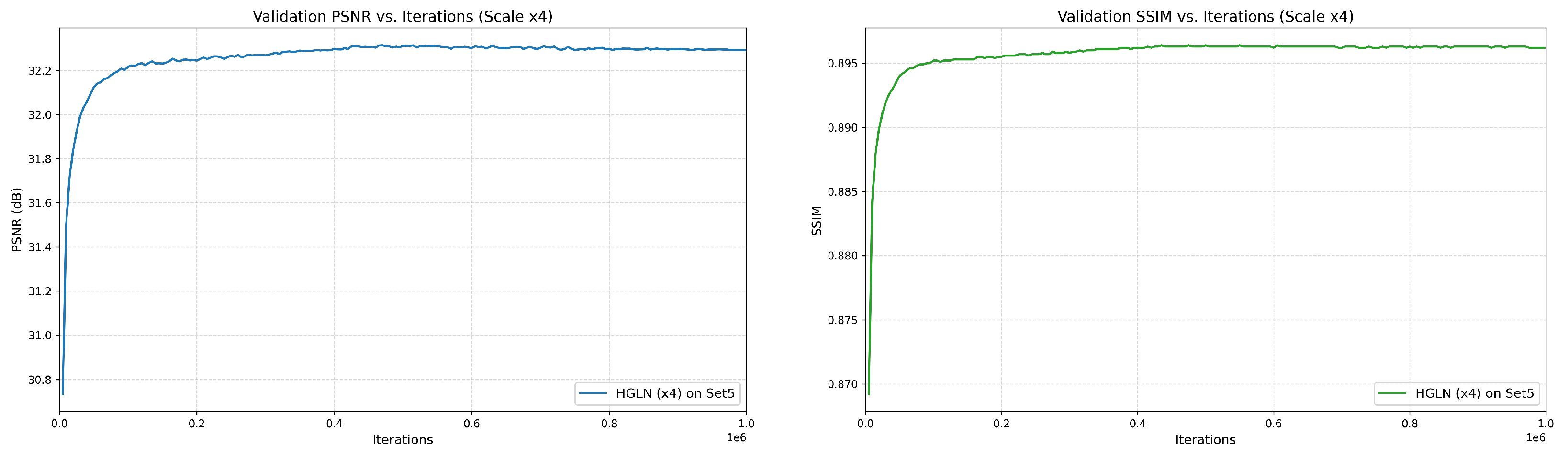
Training Stability Analysis: To verify the optimization stability of HGLN, we monitor the validation metrics throughout the training process. As illustrated in Figure 5, the validation curves for both PSNR and SSIM on the Set5 dataset ($\times 4$) demonstrate a consistent upward trajectory. Specifically, the model exhibits rapid convergence within the initial 200,000 iterations, followed by the fine-tuning of detailed textures in the subsequent stages. These smooth curves confirm that our Hybrid Gated Large-kernel architecture is robust and effectively mitigates gradient instability issues.

4.2. Datasets and Metrics

Datasets: To ensure a rigorous evaluation, we conduct experiments on widely recognized benchmark datasets. Network training utilizes the DF2K dataset, a consolidation of DIV2K [29] and Flickr2K [3], comprising a total of 3450 high-quality images with 2K resolution. This extensive collection provides diverse textural examples, facilitating the learning of robust feature representations applicable to real-world scenarios.

For testing, we assess model generalization across five standard benchmarks representing varied image complexities. Classical low-resolution scenarios are evaluated using Set5 [30] and Set14 [31]. To test performance on natural image textures and edges, we employ the B100 [32] dataset. Furthermore, to evaluate the reconstruction of complex geometric structures and aliasing-prone patterns (e.g., windows and grids), we utilize the challenging Urban100 [33] dataset. Finally, Manga109 [34] is included to verify the model’s ability to handle sharp lines and text within artistic illustrations.

Evaluation Metrics: Reconstruction fidelity is quantified using two standard metrics: Peak Signal-to-Noise Ratio (PSNR) for pixel-level accuracy and Structural Similarity Index (SSIM) for perceptual quality. Consistent with established SISR protocols, all calculations are performed on the Y channel (luminance) of the transformed YCbCr color space, as human vision is more sensitive to luminance intensity. Higher scores in both metrics indicate superior image restoration quality.

4.3. Quantitative Evaluation

We perform a comprehensive evaluation of the proposed HGLN against a wide spectrum of state-of-the-art (SOTA) lightweight SR methods. In the realm of lightweight super-resolution, a direct comparison of all methods in a single table can be misleading due to the vast differences in parameter counts and computational budgets (e.g., varying from 10 G to over 100 G Multi-Adds). To ensure a fair and structurally meaningful comparison, we categorize the competitors based on their architectural paradigms and computational intensity. Consequently, we conduct specific comparisons across three upscaling factors ($\times 2,\times 3,\times 4$), focusing on efficiency, architectural evolution, and state-of-the-art performance, respectively.

Positioning against Emerging Architectures: It is worth noting that the landscape of lightweight SR has recently evolved, with the emergence of hybrid architectures [22] and State Space Models (SSMs) such as Hi-Mamba [23]. While SSMs achieve linear complexity and impressive global modeling capabilities, they often encounter challenges regarding hardware compatibility (e.g., lack of optimized CUDA kernels for edge devices) and training stability. In contrast, HGLN is explicitly positioned as a pure CNN-based solution that rivals the receptive field of Transformers/SSMs through our proposed Hybrid Gated Large-kernel mechanism. By avoiding complex self-attention operators and state-space recursive calculations, HGLN maintains superior deployment friendliness and determinism on standard hardware, offering a pragmatic balance between the theoretical advantages of recent paradigms and the practical constraints of real-world edge applications.

Significance of Performance Margins. It is widely recognized that the field of lightweight SR has entered a phase of performance saturation. As state-of-the-art methods approach the theoretical upper bounds of reconstruction fidelity under strict parameter constraints, achieving large numerical leaps has become increasingly challenging. In this context, performance gains in the range of 0.05–0.2 dB are statistically significant and represent meaningful architectural breakthroughs rather than random variance. As demonstrated in the following comparisons, HGLN consistently achieves such margins (e.g., +0.26 dB on Manga109 $\times 2$), confirming the robustness of our design beyond statistical fluctuations.

In the following tables, the best performance is highlighted in bold.

(1) Evaluation on Scale $\times 2$: Efficiency Comparison: The $\times 2$ upscaling task generally preserves more original information, making it an ideal testing ground for ultra-lightweight architectures where every floating-point operation (FLOP) counts. In this subsection, we benchmark HGLN against methods designed for extreme efficiency (<100 G Multi-Adds), including the classic FSRCNN [35], the attention-based AIDN [8], and recent efficient operators like SAFMN [26] and ShuffleMixer [12].

As detailed in Table 1, HGLN demonstrates an unprecedented trade-off between reconstruction quality and computational cost:

• Breaking the Saturation Ceiling: On classical datasets like Set5 and Set14, performance gains are typically saturated in the lightweight domain. However, HGLN still manages to secure the top spot (38.08 dB on Set5), marginally outperforming heavier models.
• Handling High-Frequency Details: The advantage becomes substantial on the Manga109 dataset, which is replete with sharp text and high-contrast lines. While AIDN achieves a respectable 38.89 dB, HGLN surges to 39.15 dB, delivering a remarkable gain of 0.26 dB. This improvement is directly attributed to our Structure-Gated Feed-forward Network (SGFN), which injects high-frequency residuals into the gating mechanism, preventing the blurring of sharp boundaries that is common in ultra-lightweight models.
• Computational Economy: Perhaps most importantly, HGLN achieves these results with only 41 G Multi-Adds. Compared to AIDN (69 G), this represents a 40% reduction in computational load. This proves that our hybrid gated design is far more efficient at extracting informative features from low-degradation inputs than standard attention mechanisms, making it highly suitable for battery-powered devices.

Table 1. Quantitative comparison with Ultra-Lightweight Methods on Scale $\times 2$. The best results are bolded.

Method	Params [K]	GFLOPs	Set5	Set14	BSD100	Urban100	Manga109
			PSNR/SSIM	PSNR/SSIM	PSNR/SSIM	PSNR/SSIM	PSNR/SSIM
FSRCNN [35]	13	6	37.00/0.9558	32.63/0.9088	31.53/0.8920	29.88/0.9020	36.67/0.9710
AIDN [8]	323	69	38.07/0.9607	33.72/0.9192	32.18/0.8995	32.24/0.9289	38.89/0.9744
SAFMN [26]	228	52	38.00/0.9605	33.54/0.9177	32.16/0.8995	31.84/0.9256	38.71/0.9771
ShuffleMixer [12]	394	91	38.01/0.9606	33.63/0.9180	32.17/0.8995	31.89/0.9257	38.83/0.9774
HGLN(Ours)	192	41	38.08/0.9608	33.75/0.9189	32.24/0.9006	32.29/0.9298	39.15/0.9781

Table 1. Quantitative comparison with Ultra-Lightweight Methods on Scale $\times 2$. The best results are bolded.

Method	Params [K]	GFLOPs	Set5	Set14	BSD100	Urban100	Manga109
			PSNR/SSIM	PSNR/SSIM	PSNR/SSIM	PSNR/SSIM	PSNR/SSIM
FSRCNN [35]	13	6	37.00/0.9558	32.63/0.9088	31.53/0.8920	29.88/0.9020	36.67/0.9710
AIDN [8]	323	69	38.07/0.9607	33.72/0.9192	32.18/0.8995	32.24/0.9289	38.89/0.9744
SAFMN [26]	228	52	38.00/0.9605	33.54/0.9177	32.16/0.8995	31.84/0.9256	38.71/0.9771
ShuffleMixer [12]	394	91	38.01/0.9606	33.63/0.9180	32.17/0.8995	31.89/0.9257	38.83/0.9774
HGLN(Ours)	192	41	38.08/0.9608	33.75/0.9189	32.24/0.9006	32.29/0.9298	39.15/0.9781

(2) Evaluation on Scale $\times 3$: Comparison with Distillation Networks: At the intermediate $\times 3$ scale, we benchmarked HGLN against the established baseline of Information Distillation Networks, including CARN [13], IMDN [6], RFDN [7], and CFM [36]. These methods primarily rely on channel splitting and progressive refinement to reduce parameter redundancy, a paradigm that has dominated lightweight SR for years.

Table 2 highlights the architectural superiority of HGLN over these classical approaches:

• Limitations of Distillation: While IMDN and RFDN successfully reduce parameters, their reliance on small-kernel convolutions (typically $3\times 3$) inherently limits their ERF. Consequently, they struggle to capture global patterns in complex scenes. For instance, on Urban100, IMDN achieves 28.17 dB.
• Superiority of Large Kernels: In contrast, HGLN leverages the Hybrid Multi-Scale Aggregation (HMSA) module to explicitly decouple structure and detail features. By employing a modified large-kernel mechanism, HGLN outperforms IMDN by 0.10 dB (28.27 dB vs. 28.17 dB) on Urban100.
• Parameter Efficiency: This performance gain is particularly impressive given that HGLN uses only 28% of the parameters (196K vs. 703K) required by IMDN. Similarly, compared to RFDN, which is an optimized version of IMDN, HGLN maintains a clear lead in both PSNR and SSIM across all datasets. This confirms that our large-kernel strategy provides a more effective mechanism for feature representation than traditional distillation blocks, offering a better “Pareto frontier” between model size and performance.

Table 2. Quantitative comparison with classic distillation methods in terms of Scale $\times 3$. HGLN outperforms these baselines with significantly fewer parameters. The best results are bolded.

Method	Params [K]	GFLOPs	Set5	Set14	BSD100	Urban100	Manga109
			PSNR/SSIM	PSNR/SSIM	PSNR/SSIM	PSNR/SSIM	PSNR/SSIM
CARN [13]	1592	119	34.29/0.9255	30.29/0.8407	29.06/0.8034	28.06/0.8493	33.50/0.9440
IMDN [6]	703	72	34.36/0.9270	30.32/0.8417	29.09/0.8046	28.17/0.8519	33.61/0.9445
RFDN [7]	541	42	34.41/0.9273	30.34/0.8420	29.09/0.8050	28.21/0.8525	33.67/0.9449
CFM [36]	319	34	34.37/0.9272	30.33/0.8419	29.09/0.8060	28.02/0.8495	33.49/0.9441
HGLN(Ours)	196	19	34.46/0.9278	30.47/0.8446	29.17/0.8070	28.27/0.8541	34.01/0.9466

Table 2. Quantitative comparison with classic distillation methods in terms of Scale $\times 3$. HGLN outperforms these baselines with significantly fewer parameters. The best results are bolded.

Method	Params [K]	GFLOPs	Set5	Set14	BSD100	Urban100	Manga109
			PSNR/SSIM	PSNR/SSIM	PSNR/SSIM	PSNR/SSIM	PSNR/SSIM
CARN [13]	1592	119	34.29/0.9255	30.29/0.8407	29.06/0.8034	28.06/0.8493	33.50/0.9440
IMDN [6]	703	72	34.36/0.9270	30.32/0.8417	29.09/0.8046	28.17/0.8519	33.61/0.9445
RFDN [7]	541	42	34.41/0.9273	30.34/0.8420	29.09/0.8050	28.21/0.8525	33.67/0.9449
CFM [36]	319	34	34.37/0.9272	30.33/0.8419	29.09/0.8060	28.02/0.8495	33.49/0.9441
HGLN(Ours)	196	19	34.46/0.9278	30.47/0.8446	29.17/0.8070	28.27/0.8541	34.01/0.9466

(3) Evaluation on Scale $\times 4$: Comparison with SOTA Methods. The $\times 4$ scale presents the most severe degradation challenge, requiring the network to hallucinate substantial missing high-frequency details. Here, we conduct a definitive comparison against the most competitive State-of-the-Art (SOTA) methods, including the sparsity-based SMSR [10], the attention-based DIPNet [11], and we revisit the strong competitors ShuffleMixer [12] and SAFMN [26] to demonstrate HGLN’s robustness under extreme conditions.

Table 3 validates that HGLN achieves a dominating performance on complex benchmarks, effectively solving the “large receptive field vs. low complexity” dilemma.

• Robustness on Complex Structures: On the Urban100 dataset, which contains rich architectural details and repeating grids, HGLN reaches 26.22 dB, consistently surpassing DIPNet (26.16 dB) and ShuffleMixer (26.08 dB). The improvement of 0.14 dB over ShuffleMixer is critical in lightweight SR, indicating that our gating mechanism effectively suppresses noise while the large kernels capture the long-range dependencies necessary for reconstructing regular grids.
• Structural Integrity: On Manga109, HGLN achieves 30.85 dB, exceeding ShuffleMixer (30.65 dB) by a remarkable margin of 0.20 dB. The high SSIM score (0.9112) further confirms that our dual-path processing successfully maintains the structural integrity of lines, avoiding the aliasing artifacts common in other methods.
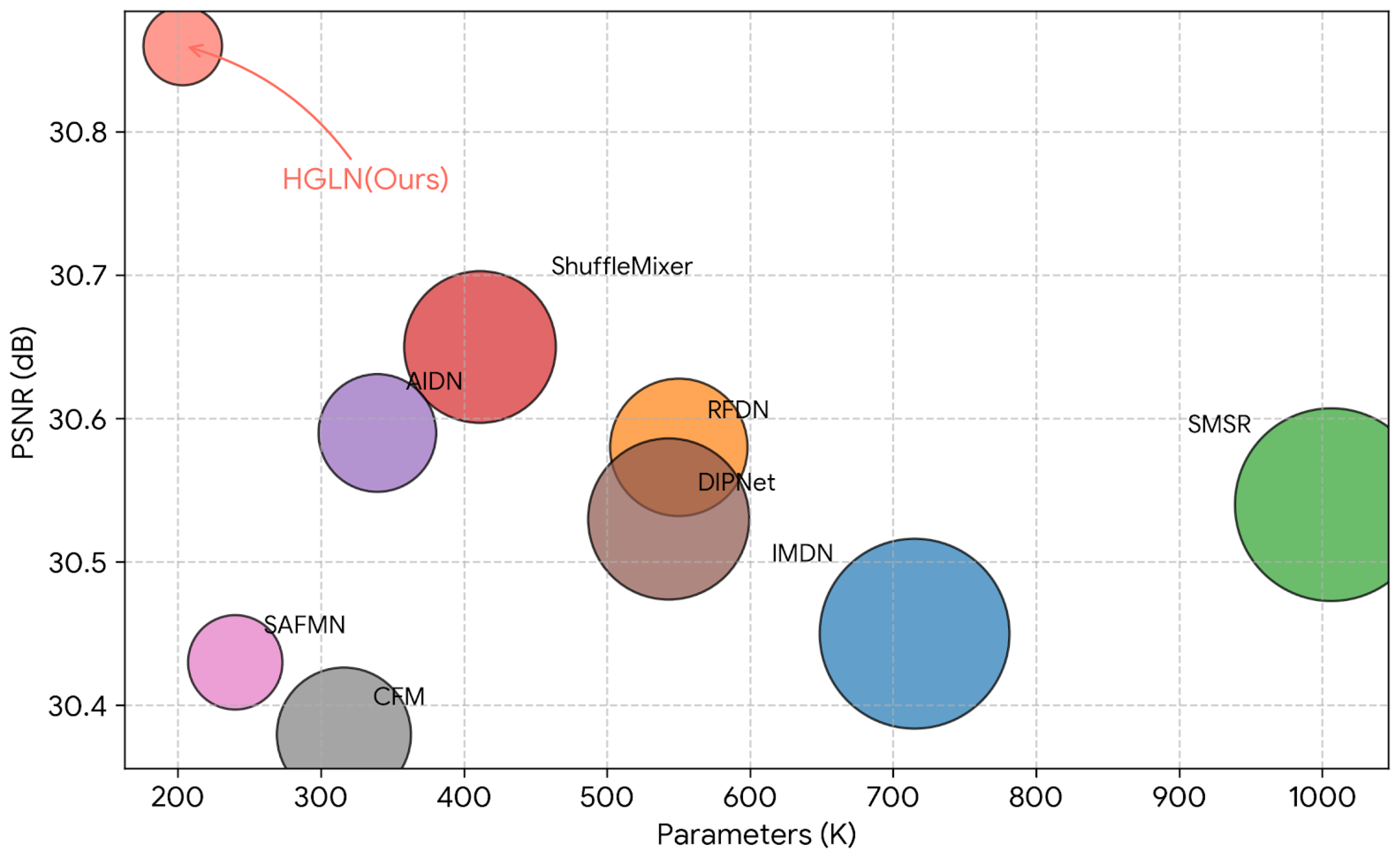
• Deployment Feasibility: Most importantly, HGLN achieves these SOTA results with the lowest computational cost among all deep methods—only 11 G Multi-Adds. This represents a 31% reduction compared to DIPNet (16G) and a staggering 60% reduction compared to ShuffleMixer (28G). This extreme efficiency implies that HGLN can be deployed on edge devices with significantly lower latency and power consumption, marking a substantial step forward for practical SISR applications.

Table 3. Quantitative comparison with State-of-the-Art (SOTA) Methods on Scale $\times 4$. HGLN achieves the best performance on complex datasets (Urban100, Manga109) with the lowest computational cost. The best results are bolded.

Method	Params [K]	GFLOPs	Set5	Set14	BSD100	Urban100	Manga109
			PSNR/SSIM	PSNR/SSIM	PSNR/SSIM	PSNR/SSIM	PSNR/SSIM
SMSR [10]	1006	42	32.12/0.8932	28.55/0.7808	27.55/0.7351	26.11/0.7868	30.54/0.9085
SAFMN [26]	240	14	32.18/0.8948	28.60/0.7813	27.58/0.7359	25.97/0.7809	30.43/0.9063
DIPNet [11]	543	16	32.20/0.8950	28.58/0.7811	27.59/0.7364	26.16/0.7879	30.53/0.9087
ShuffleMixer [12]	411	28	32.21/0.8953	28.66/0.7827	27.61/0.7366	26.08/0.7835	30.65/0.9093
HGLN(Ours)	203	11	32.29/0.8963	28.73/0.7842	27.64/0.7384	26.22/0.7879	30.85/0.9112

Table 3. Quantitative comparison with State-of-the-Art (SOTA) Methods on Scale $\times 4$. HGLN achieves the best performance on complex datasets (Urban100, Manga109) with the lowest computational cost. The best results are bolded.

Method	Params [K]	GFLOPs	Set5	Set14	BSD100	Urban100	Manga109
			PSNR/SSIM	PSNR/SSIM	PSNR/SSIM	PSNR/SSIM	PSNR/SSIM
SMSR [10]	1006	42	32.12/0.8932	28.55/0.7808	27.55/0.7351	26.11/0.7868	30.54/0.9085
SAFMN [26]	240	14	32.18/0.8948	28.60/0.7813	27.58/0.7359	25.97/0.7809	30.43/0.9063
DIPNet [11]	543	16	32.20/0.8950	28.58/0.7811	27.59/0.7364	26.16/0.7879	30.53/0.9087
ShuffleMixer [12]	411	28	32.21/0.8953	28.66/0.7827	27.61/0.7366	26.08/0.7835	30.65/0.9093
HGLN(Ours)	203	11	32.29/0.8963	28.73/0.7842	27.64/0.7384	26.22/0.7879	30.85/0.9112

4.4. Qualitative Architectural Analysis

While quantitative metrics demonstrate the performance superiority of HGLN, it is equally important to understand the architectural distinctions that lead to these improvements. In

Table 4. Qualitative comparison between HGLN and state-of-the-art lightweight SR methods.

Method	Core Paradigm	Kernel	Attention	Key Design
IMDN [6]	Distillation	$3\times 3$	CCA	Progressive feature splitting
RFDN [7]	Distillation	$3\times 3$	ESA	Residual feature distillation
SMSR [10]	Sparsity	$3\times 3$	Sparse Mask	Pruning in smooth regions
ShuffleMixer [12]	Efficient Operator	$7\times 7$ (Sim.)	Projection	Channel shuffle mixing
SAFMN [26]	Modulation	$3\times 3$	Scaled	Spatially adaptive modulation
HGLN (Ours)	Hybrid Gated	$9\times 9$	Dual-Gated	Decoupled structure & detail

, we provide a qualitative comparison between HGLN and other representative lightweight methods.

As summarized in the table, most existing lightweight networks (e.g., IMDN, RFDN, SAFMN) rely on small-kernel convolutions (typically $3\times 3$) and standard attention mechanisms. Although efficient, these designs inherently limit the effective receptive field. In contrast, HGLN introduces a hybrid paradigm that explicitly decouples structural and detailed features. By leveraging large-kernel convolutions ($9\times 9$) and the structure-aware SGFN, HGLN effectively balances long-range dependency capture with local detail preservation.

4.5. Model Complexity Analysis

In real-world scenarios, particularly for mobile and edge devices, the deployment of Super-Resolution models is constrained not only by reconstruction quality but also by hardware limitations such as memory bandwidth and battery capacity. Therefore, we conduct a deep analysis of model complexity from two distinct perspectives: Parameter Efficiency (storage footprint) and Computational Efficiency (inference latency and power consumption).

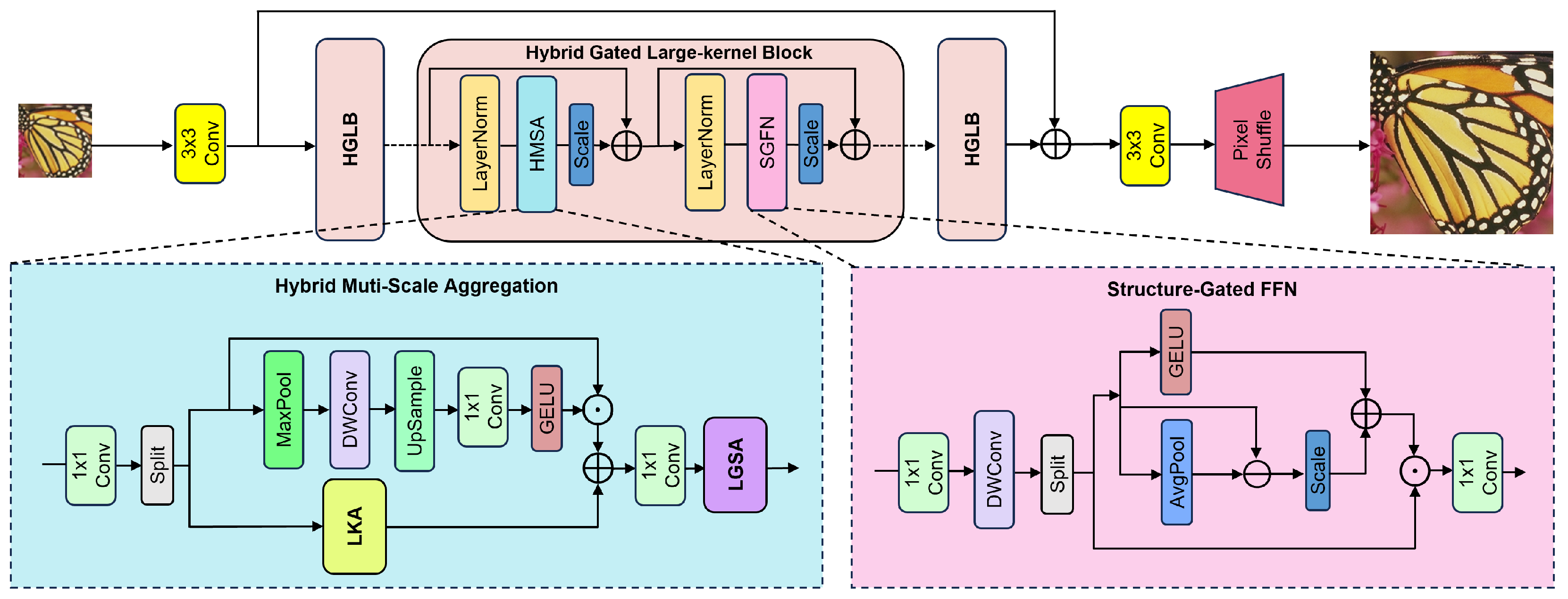
Parameter Efficiency: As illustrated in the “Params” column of our comparison tables, HGLN maintains an extremely compact size. At scale $\times 4$, the model contains only 203 K parameters. When compared to the attention-based AIDN (339 K), HGLN reduces the model size by approximately 40%. More strikingly, compared to the pruning-based SMSR (1006 K), which relies on sparsity to speed up inference but requires a large number of parameters to maintain capacity, HGLN requires merely 20% of its parameters. This compactness is attributed to our HMSA module, which employs a split–transform–merge strategy. By processing structural and detail features in parallel streams with halved channels, we significantly reduce feature redundancy without sacrificing representational power.

Computational Efficiency: While parameter count determines storage, the number of Multi-Adds (FLOPs) is a more direct indicator of execution speed and energy efficiency. HGLN demonstrates the lowest computational cost among all compared deep networks. Calculating on a $1280\times 720$ output at $\times 4$ scale, HGLN consumes only 11 G Multi-Adds.

• Compared to DIPNet (16 G), which is designed for efficiency, HGLN achieves a 31% reduction in computations.
• Compared to ShuffleMixer (28 G), HGLN reduces the workload by a massive 60%.
• Even when pitted against the highly optimized SAFMN (14 G), our model saves roughly 21% of computations while delivering higher PSNR scores (e.g., +0.25 dB on Urban100).

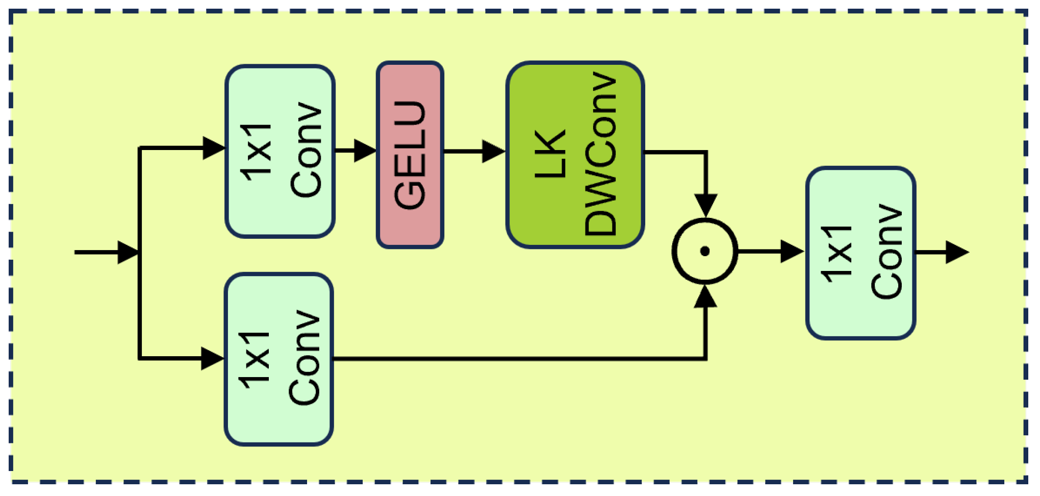
This ultra-low computational cost is primarily achieved by our use of large-kernel depth-wise convolutions within the LKA branch, which expands the receptive field with negligible arithmetic cost compared to standard dense convolutions.

Consequently, HGLN achieves a superior Pareto frontier between performance and complexity. The combination of minimal storage requirements and ultra-low FLOPs makes HGLN an ideal candidate for real-time applications on resource-constrained edge devices, ensuring longer battery life and lower heat generation during high-fidelity image reconstruction.

4.6. Visual Quality Comparison

While quantitative metrics like PSNR and SSIM provide an objective measure of reconstruction accuracy, they do not always align perfectly with human perceptual judgment. Therefore, we further evaluate the perceptual quality of the reconstructed images by inspecting the restoration results on challenging benchmarks.

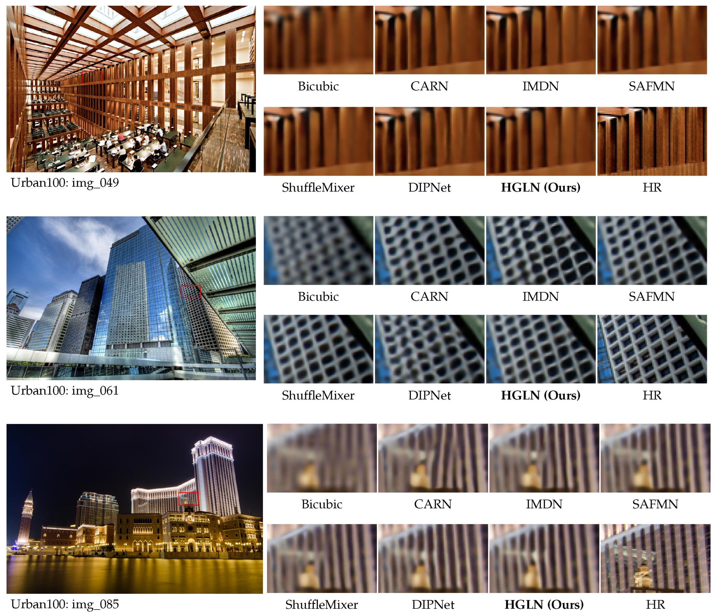
(1) Restoration of Architectural Structures: Restoring repetitive geometric patterns remains a significant challenge, often leading to aliasing artifacts. Figure 6 presents comparisons on the Urban100 dataset. It is evident that small-kernel-based methods like IMDN and SAFMN fail to capture global periodic information, resulting in severe Moiré patterns and structural distortions in img_049 and img_061. In contrast, HGLN leverages the HMSA module to effectively capture long-range dependencies. By expanding the effective receptive field, our model successfully resolves aliasing ambiguities, restoring sharp and correct grid structures that closely match the Ground Truth.

(2) Restoration of Text and Characters: In addition to geometric structures, the legibility of text is a critical metric for real-world SR applications, such as document restoration and screen content enhancement. Figure 7 illustrates the performance on text-heavy images from Manga109 (“Hamlet”) and Set14 (“ppt3”).

• Complex Artistic Text: As shown in the top row (“Hamlet”), the comic text contains varying stroke widths and high-contrast edges. Competitors like ShuffleMixer and IMDN tend to produce over-smoothed results, where distinct strokes merge into “mushy” blobs, severely compromising readability. This occurs because simple channel-mixing operations often act as low-pass filters, discarding high-frequency edge information. However, HGLN maintains the structural integrity of the strokes, delivering clear separation between characters.
• Screen Content Text: Similarly, in the “ppt3” example (bottom row), which simulates a digital screen scenario with small fonts, HGLN exhibits a distinct advantage. While other methods introduce ringing artifacts (ghosting shadows around letters) or fail to reconstruct the sharp corners of the alphabet, HGLN effectively suppresses these artifacts.

Figure 7. Visual comparison of text reconstruction capabilities ($\times 4$). The top row shows the results on Hamlet (Manga109), and the bottom row shows the results on ppt3 (Set14). By arranging the comparisons vertically, we highlight the fine-grained details. HGLN (Ours) demonstrates superior performance in recovering sharp character edges and suppressing blurring artifacts in both scenarios.

Figure 7. Visual comparison of text reconstruction capabilities ($\times 4$). The top row shows the results on Hamlet (Manga109), and the bottom row shows the results on ppt3 (Set14). By arranging the comparisons vertically, we highlight the fine-grained details. HGLN (Ours) demonstrates superior performance in recovering sharp character edges and suppressing blurring artifacts in both scenarios.

This superior text restoration capability is attributed to our SGFN. By explicitly gating the feature flow with high-frequency residuals, SGFN ensures that sharp boundaries are preserved and enhanced, making HGLN highly robust for restoring content with rich semantic information.

4.7. Ablation Study

To thoroughly investigate the effectiveness of the proposed HGLN, we conduct comprehensive ablation studies on the challenging Urban100 dataset ($\times 4$). All ablation models are trained on the DF2K dataset. To balance experimental efficiency and reliability, we adopt a rapid validation protocol: all variants are trained for 200,000 iterations with a batch size of 32 using the Adam optimizer (${\beta }_1=0.9,{\beta }_2=0.999$). The initial learning rate is set to $2\times {10}^{-4}$ and halved at 100,000 iterations. Except for the specific module being tested, all other configurations remain consistent with the final HGLN model to ensure fair comparisons.

(1)

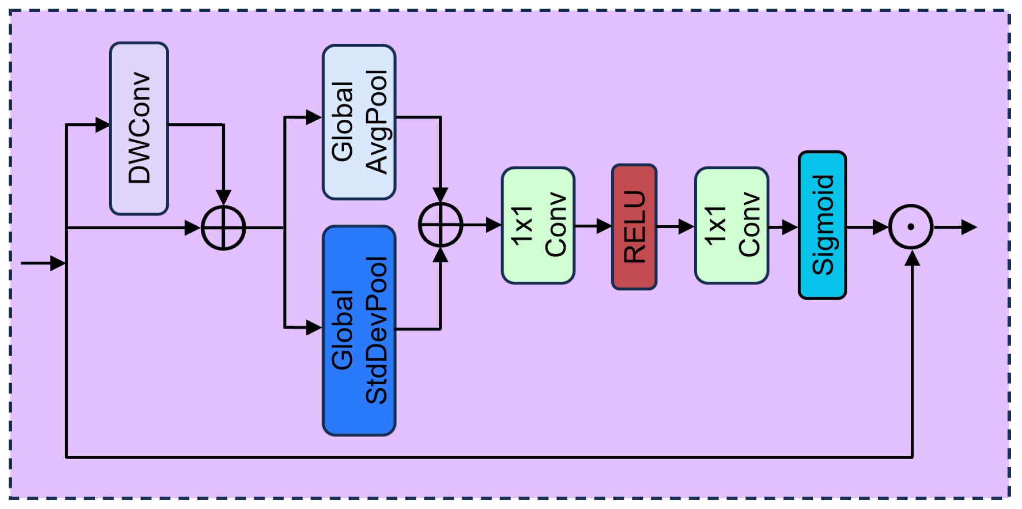
Effectiveness of Core Components: The architectural superiority of HGLN stems from its three novel components: the Hybrid Multi-Scale Aggregation (HMSA) module, the Local–Global Synergistic Attention (LGSA), and the Structure-Gated Feed-forward Network (SGFN). To validate their individual contributions, we replace them with their standard counterparts in the existing literature:

• HMSA → LKA (Large Kernel Attention) [16];
• LGSA → SE-Block (Squeeze-and-Excitation) [18];
• SGFN → GDFN (Gated-Dconv Feed-forward Network) [25].

The quantitative results are summarized in

Table 5. Ablation study on core components. Our proposed modules (HMSA, LGSA, SGFN) are replaced by standard baselines (LKA, SE-Block, GDFN) to verify their effectiveness. The best results are bolded.

Model Variant	Param. (K)	M-Adds (G)	PSNR (dB)	SSIM
HMSA → LKA	126.62	6.96	25.72	0.7730
LGSA → SE-Block	200.35	10.68	26.01	0.7816
SGFN → GDFN	202.73	10.82	26.02	0.7821
HGLN (Full)	203.30	10.82	26.04	0.7827

. First, replacing HMSA with the standard LKA leads to a drastic performance degradation of 0.32 dB in PSNR (25.72 dB vs. 26.04 dB). Although LKA significantly reduces the parameter count to 126.62 K, its reliance on simple depth-wise convolutions limits its ability to capture complex feature correlations. In contrast, our HMSA leverages a dual-path design to aggregate both local identity and long-range dependencies, proving indispensable for high-fidelity reconstruction. Second, replacing LGSA with the standard SE-Block results in a 0.03 dB drop. While the SE-Block captures global channel interdependencies, it neglects local statistical information. LGSA addresses this by incorporating local variance, which is crucial for texture awareness. Third, the SGFN outperforms the standard GDFN by 0.02 dB. This confirms that the proposed structure-aware gating mechanism is more effective at preserving high-frequency details than the conventional gating used in Restormer.

(2)

Internal Mechanisms of LGSA and SGFN: We further delve into the micro-designs of our attention and feed-forward modules. specifically, we investigate the necessity of the standard deviation branch in LGSA (w/o Std) and the high-frequency injection path in SGFN (w/o HF-Inject).

As shown in

Table 6. Ablation study on the internal mechanisms. We investigate the impact of the standard deviation branch in LGSA and the High-Frequency Injection in SGFN. The best results are bolded.

Module	Variant	PSNR (dB)	SSIM
LGSA	w/o Std (Mean Only)	26.02	0.7819
	Full LGSA	26.04	0.7827
SGFN	w/o HF-Inject	26.03	0.7823
	Full SGFN	26.04	0.7827

, removing the standard deviation branch (‘w/o Std’) leads to a performance drop of 0.02 dB. Theoretically, while mean pooling extracts background intensity, the standard deviation serves as a contrast detector, capturing the richness of local textures. The combination of both statistics enables robust feature recalibration. Similarly, omitting the High-Frequency Injection (‘w/o HF-Inject’) results in a 0.01 dB degradation. This injection strategy acts as a structural prior, guiding the network to focus on edges and boundaries. Considering that these components introduce virtually zero computational overhead, they are highly cost-effective designs for enhancing perceptual quality.

(3)

Impact of Kernel Size: The kernel size k in the HMSA module determines the ERF of the network. We analyze the trade-off between receptive field expansion and optimization difficulty by varying k from 5 to 11.

The results in

Table 7. Ablation study on the kernel size (k) of the HMSA module. The results indicate that $9\times 9$ provides the optimal trade-off. The best results are bolded.

Kernel ($\mathit{k}\times \mathit{k}$)	Param. (K)	M-Adds (G)	PSNR (dB)	SSIM
$5\times 5$	187.18	9.90	25.99	0.7809
$7\times 7$	194.09	10.29	26.03	0.7821
9 × 9	203.30	10.82	26.04	0.7827
$11\times 11$	214.82	11.49	25.99	0.7816

reveal an interesting trend. Increasing k from 5 to 9 yields consistent gains, improving PSNR from 25.99 dB to a peak of 26.04 dB. This validates that larger kernels effectively capture long-range dependencies, which are crucial for hallucinating high-frequency architectural details in Urban100. However, further enlarging k to 11 brings no improvement, with performance dropping back to 25.99 dB. This suggests that excessively large kernels may introduce optimization difficulties due to sparse correlations or vanishing gradients in depth-wise convolutions. Consequently, we adopt $k=9$ as the optimal setting, achieving the best balance between model complexity (203.30 K parameters) and restoration fidelity.

4.8. Internal Mechanism and Interpretability

In this section, we provide a deeper investigation into the working mechanism of HGLN from two perspectives: the ERF and the intermediate feature response.

4.8.1. Effective Receptive Field Analysis

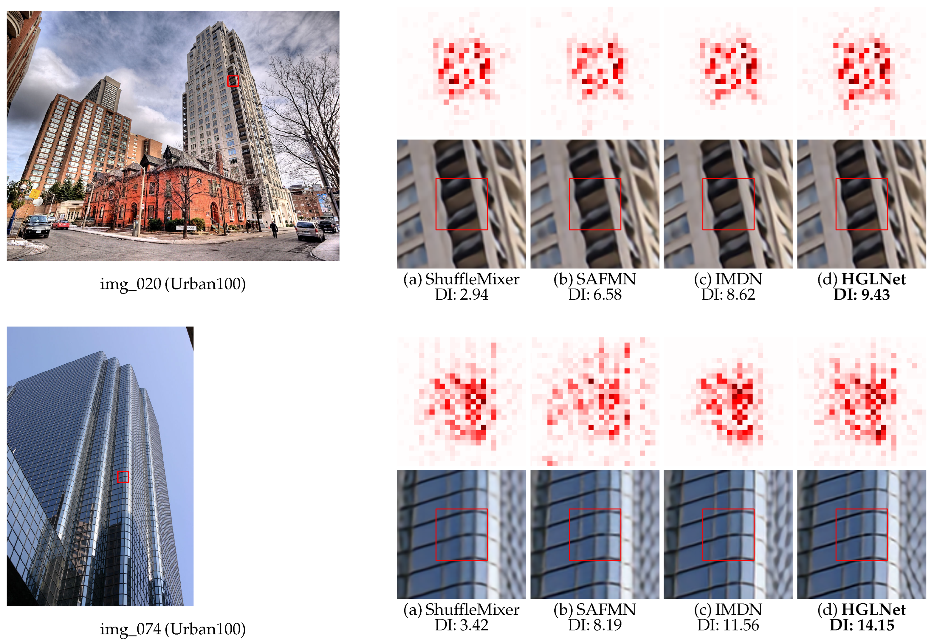
To verify whether HGLN truly utilizes long-range dependencies as designed, we employ the Local Attribution Map (LAM) [37] method. LAM visualizes the pixel usage of the input image that contributes the most to the reconstruction of a specific patch. Figure 8 compares the LAM results and the corresponding Diffusion Index (DI) [37] of HGLN against state-of-the-art lightweight models (ShuffleMixer, SAFMN, and IMDN) on the Urban100 dataset.

It is important to note that the Diffusion Index (DI) serves as a critical quantitative metric for the scope of information utilization. Mathematically, DI quantifies the spatial distribution of contributing pixels in the input image. A higher DI value indicates a broader Effective Receptive Field (ERF), implying that the model is capable of harnessing a wider-ranging spatial context to reconstruct local details. In the ill-posed problem of super-resolution, local information is often insufficient to recover missing high-frequency textures. Therefore, a high DI score signifies that the network can successfully perform non-local reasoning, aggregating useful features (such as repetitive geometric patterns) from distant regions to correct aliasing and hallucinate realistic details.

• Wider Effective Receptive Field (High DI vs. Low DI): As illustrated in Figure 8, the red areas represent the pixels that contribute significantly to the reconstruction. It is evident that the attribution maps of competitive models like ShuffleMixer and SAFMN are confined to a very small local region (e.g., ShuffleMixer only achieves a DI of 2.94 on img_020). This low DI suggests a “tunnel vision” limitation: these models rely heavily on immediate neighboring pixels and fail to utilize surrounding texture information effectively, often leading to blurred edges in complex structures.
• Global Dependency Capture: In contrast, HGLN activates a significantly broader range of pixels, extending along the direction of the structural textures. On img_074, HGLN achieves a remarkable DI score of 14.15, which is nearly $4\times$ higher than that of ShuffleMixer (3.42). This substantial increase in DI confirms that our hybrid gated large-kernel design successfully breaks the locality constraint of standard CNNs, enabling the model to capture long-range dependencies that are essential for consistent structural restoration.

This visualization provides strong empirical evidence that our large-kernel hybrid design successfully expands the ERF. By aggregating information from a wider context, HGLN can reconstruct repetitive patterns more accurately, avoiding the hallucinations common in local-window-based methods.

4.8.2. Intermediate Feature Visualization

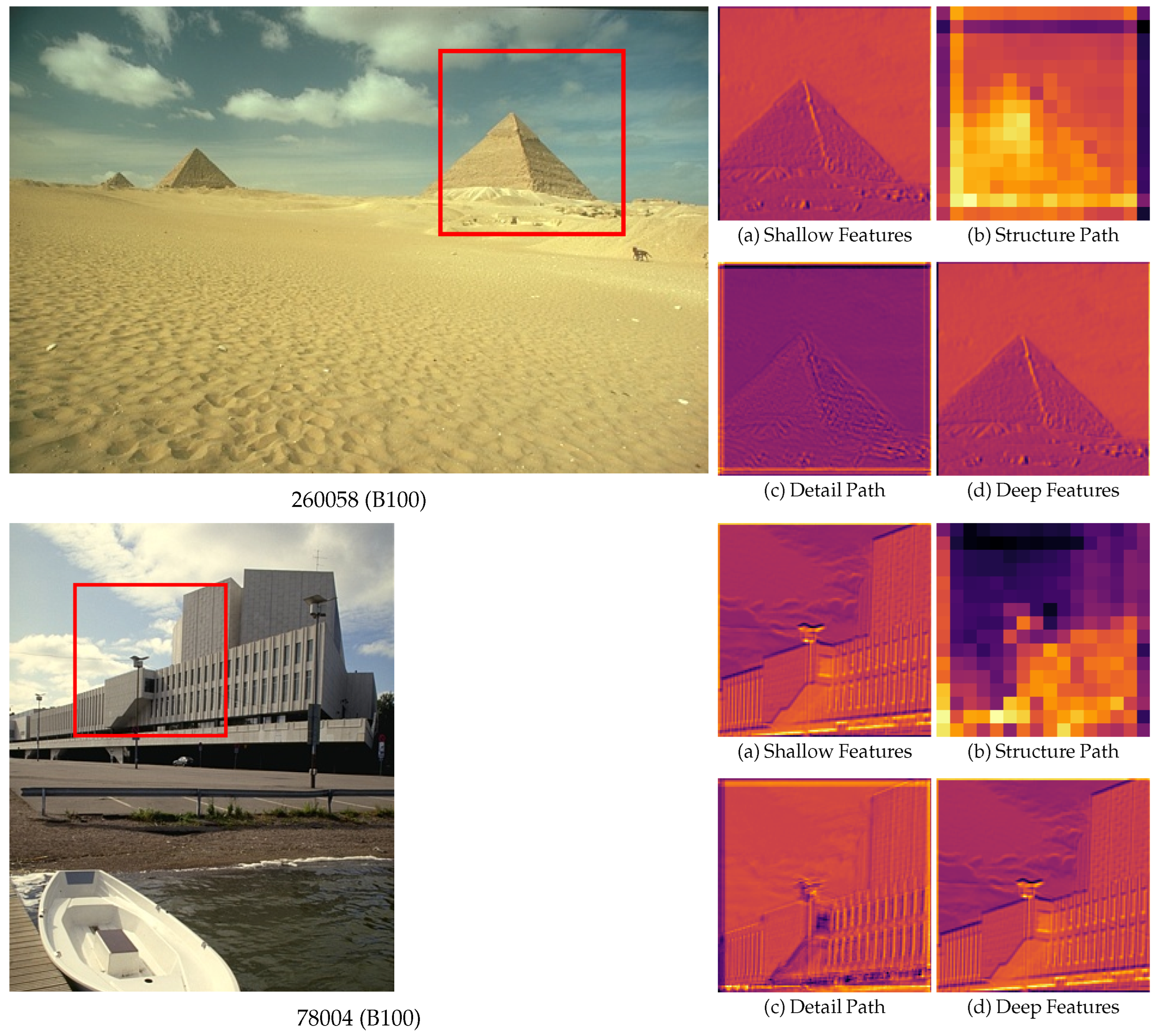
To further validate the frequency decoupling mechanism of our proposed Hybrid Multi-Scale Aggregation (HMSA) module, we visualize the intermediate feature maps produced by its two internal pathways: the Structure Path and the Detail Path.

As shown in Figure 9, we visualize the feature responses on samples from the BSD100 dataset:

• Structure Path (Low-Frequency): The Structure Path (Figure 9b) mainly activates on the global shapes and skeletal outlines of the objects (e.g., the building edges in the bottom row). It effectively suppresses high-frequency noise, confirming its role in capturing structural priors.
• Detail Path (High-Frequency): Conversely, the Detail Path (Figure 9c), powered by Large Kernel Attention (LKA), exhibits strong activation in regions with rich textures (e.g., the pyramid surface in the top row). This demonstrates that the large-kernel design is crucial for preserving fine-grained details.

The distinct activation patterns between the two paths verify the effectiveness of our hybrid strategy in separating and processing different frequency components.

Figure 9. Visualizations of intermediate feature maps. Top Row: Sample 260058 (landscape scene), showing texture details on the pyramid surface activated by the Detail Path. Bottom Row: Sample 78004 (portrait scene), highlighting the structural edges of the building in the Structure Path. In each group, the left panel shows the HR image where the red box indicates the Region of Interest (ROI), and (a–d) visualize the shallow, structure, detail, and deep features, respectively.

Figure 9. Visualizations of intermediate feature maps. Top Row: Sample 260058 (landscape scene), showing texture details on the pyramid surface activated by the Detail Path. Bottom Row: Sample 78004 (portrait scene), highlighting the structural edges of the building in the Structure Path. In each group, the left panel shows the HR image where the red box indicates the Region of Interest (ROI), and (a–d) visualize the shallow, structure, detail, and deep features, respectively.

5. Conclusions

In this paper, we proposed a novel HGLN for efficient and accurate single-image super-resolution. Addressing the critical challenge of balancing computational efficiency with reconstruction fidelity, we introduced a suite of architectural innovations designed to maximize the effective receptive field while minimizing parameter redundancy. Specifically, the HMSA module decouples features into structural and detailed streams, utilizing large-kernel convolutions to explicitly capture long-range dependencies and global periodic patterns. Meanwhile, the LGSA overcomes the limitations of standard global pooling by incorporating local context embeddings and dual-statistic descriptors, enabling highly discriminative feature recalibration. Furthermore, the SGFN leverages a high-frequency injection mechanism to adaptively emphasize edge and texture restoration. Extensive quantitative experiments on standard benchmarks demonstrate that HGLN achieves superior performance compared to state-of-the-art lightweight methods. Qualitative evaluations, including visual comparisons on urban scenes and text, along with Local Attribution Map (LAM) analysis, further empirically validate that HGLN successfully resolves aliasing artifacts and utilizes a broader range of input pixels for reconstruction.

Limitations and Future Research Directions

Despite the promising performance of HGLN, challenges and avenues remain for future exploration:

• Generalization to Real-World Degradations: Currently, HGLN is optimized for the standard bicubic degradation model, which assumes a noise-free input. However, in practical applications—especially under low-light conditions—images are inevitably corrupted by sensor thermal noise, typically modeled as Additive White Gaussian Noise (AWGN). HGLN is designed to aggressively recover high-frequency details via the SGFN module; there is a potential risk that the network might interpret random noise patterns as valid textures, leading to artifact amplification. In this work, we have not exhaustively evaluated this trade-off between detail restoration and noise suppression. In the future, we plan to address this by incorporating Gaussian noise into the training data augmentation pipeline or exploring a joint denoising-and-super-resolution framework to enhance the model’s robustness against sensor noise.
• Hardware Optimization for Large Kernels: Although HGLN maintains a low parameter count, the use of large-kernel convolutions (e.g., $9\times 9$) can sometimes lead to higher memory access costs on specific hardware accelerators compared to small kernels. Future work will focus on optimizing the inference efficiency through structural re-parameterization techniques or model quantization (e.g., INT8 quantization) to facilitate deployment on edge devices.
• Extension to Video Super-Resolution: HGLN’s strong ability to capture structural information makes it a potential candidate for video tasks. We plan to explore the use of temporal alignment modules to adapt the HGLN architecture for Video Super-Resolution (VSR), aiming to maintain temporal consistency while restoring high-frequency details.