SRNN: Surface Reconstruction from Sparse Point Clouds with Nearest Neighbor Prior

Abstract

Surface reconstruction from 3D point clouds has a wide range of applications. In this paper, we focus on the reconstruction from raw, sparse point clouds. Although some existing methods work on this topic, the results often suffer from geometric defects. To solve this problem, we propose a novel method that optimizes a neural network (referred to as signed distance function) to fit the Signed Distance Field (SDF) from sparse point clouds. The signed distance function is optimized by projecting query points to its iso-surface accordingly. Our key idea is to encourage both the direction and distance of projection to be correct through the supervision provided by a nearest neighbor prior. In addition, we mitigate the error propagated from the prior function by augmenting the low-frequency components in the input. In our implementation, the nearest neighbor prior is trained with a large-scale local geometry dataset, and the positional encoding with a specified spectrum is used as a regularization for the optimization process. Experiments on the ShapeNetCore dataset demonstrate that our method achieves better accuracy than SDF-based methods while preserving smoothness.

1. Introduction

Surface reconstruction is a fundamental problem in computer graphics and 3D vision, involving fitting a continuous surface to a discrete set of points. With the advancement of scanning devices and point cloud reconstruction methods, sparse point clouds are now accessible to more people and offer various possibilities for downstream applications, such as model reconstruction, generation, 3D printing, and more. However, reconstructing meshes from sparse point clouds without normal vectors is challenging for reconstruction pipelines designed for dense inputs, particularly in maintaining smoothness and robustness when generating the underlying surface.

Sparse point clouds produced by a completion/generation method typically contain 2048 or 4096 points (some methods provide up to 16k points through up-sampling but not natively). However, traditional reconstruction methods are evaluated with about 16k to 100k points [1,2,3,4,5,6]. These traditional methods designed for dense point clouds are not suitable for sparse point clouds. Recently, several reconstruction methods have been proposed to convert sparse data into 3D meshes. Based on the reconstruction pipeline of Neural-Pull [1], OSP [7] introduces a data-driven on-surface prior designed for sparse point clouds as supervision. GeoUDF [8] and SuperUDF [9] attempt to directly predict an Unsigned Distance Field (UDF) instead of an SDF with a neural network, making it much faster to reconstruct a field but harder to extract a high-quality surface. In summary, methods based on neural SDF representations exhibit weakness in accuracy, while methods predicting UDFs struggle with geometric defects (e.g., producing spikes).

To reconstruct more accurate and smoother surfaces from sparse point clouds, we propose an SDF-based reconstruction pipeline to get smooth and watertight (if it is closed) meshes. Based on the observation of existing methods and their results, we address a fundamental problem: How to constrain values and signs without explicit knowledge about point normals or surface directions? To solve this issue, we introduce a data-driven local geometric prior, the nearest neighbor prior, as a supervision for an Multilayer Perceptron (MLP) to fit the object’s SDF. It predicts the nearest neighbor of a query point on the underlying surface by implicitly fitting a local surface patch. Since the MLP fits the prior rather than the ground truth values of the SDF, systematic errors inherited from the prior inevitably persist in the reconstruction. To mitigate the inherent errors propagated from the prior and regularize the MLP against overfitting to the prior, we insert a specially designed positional encoding (PE) layer into the MLP as a data augmentation. This PE layer encodes input values with a set of low-frequency sine and cosine functions, effectively reducing high-frequency error inherited from the local prior function by augmenting the low-frequency components in the input. We implement a projection-based optimization pipeline inspired by [1] with our nearest neighbor prior and PE layer.

We evaluate our method on the ShapeNetCore dataset. The comparison shows that our approach produces meshes with better accuracy compared to SDF-based methods, and achieves significantly better geometric quality than the UDF-based method while preserving competitive precision. Ablation studies about the prior function and PE layer validate their effectiveness while demonstrating that the PE layer makes the MLP converge more stably. Our contributions are listed below.

• We introduce the nearest neighbor prior, a novel data-driven, local geometric prior as supervision for optimizing a neural network to fit SDFs from sparse point clouds without normal vectors.
• We introduce an idea to augment low-frequency components implemented by a positional encoding layer, serving as a regularization of the optimization process.
• We validate the effectiveness of our method through experiments on diverse objects and extensive ablation studies.

2. Related Works

2.1. Surface Reconstruction from Point Cloud

Surface reconstruction aims to approximate continuous surfaces from discrete point samples, a fundamentally ill-posed problem due to the vast solution space. This inherent ill-posedness necessitates regularization strategies in all reconstruction methods to ensure smoothness or fairness of the resulting surface [10,11].

Early analytical approaches leverage mathematical constructs such as Voronoi diagrams [12], parametric surfaces [13], and Poisson equations [2,14] to generate triangle meshes or indicator fields, where parametric continuity ($C^1$ or $C^2$) is inherently guaranteed by these formulations. Template-based techniques like RANSAC [15] and Polyfit [16] assemble parametric primitives (e.g., planes, cubes, cones) to model underlying surfaces. While individual primitives maintain simplicity and geometric perfection, their combinations may exhibit artifacts such as misaligned edges/faces and face limitations in representing complex shapes through finite primitive types. The continuity of neural networks as universal function approximators has enabled new reconstruction paradigms. Atzmon et al. [17] establish that MLPs can represent arbitrary piecewise-linear surfaces (polygon meshes), a capability later extended to convolutional neural networks (CNNs) by Gadelha et al. [4]. The Deep Geometric Prior [3] implements this concept through overlapping surface patches individually modeled by MLPs. Alternative approaches like Point2Mesh [18] and SAIL-S3 [19] employ multiple MLPs to fit implicit field components rather than explicit surface patches. Global feature-based learning methods [20,21,22] replace optimization for each object with inference of pre-trained models to accelerate the reconstruction process, though they face challenges in rotation invariance [23] and generalization to unseen object categories. To address these limitations, recent local-feature approaches have emerged, including Meshlet [23], PatchNets [6], IF-Nets [24], ConvOccNet [25], SSRNet [5], and Neural Kernel [26], which prioritize localized geometric characteristics over global representations.

The methods described above have limitations when applied to sparse point clouds due to their reliance on dense sampling. Early approaches exclusively utilized dense point clouds (typically containing 16k to 100k points) with normal vectors, followed by methods supporting normal-free dense point clouds. Recently, several methods for sparse point clouds have emerged. Meshlet [23] can reconstruct from 5k points, while subsequent methods demonstrate compatibility with even sparser inputs. A projection-based optimization schema was introduced by Neural Pull [1] and later adopted by OSP [7], which has proven effective for sparse point cloud processing. Neural Pull was originally developed for dense point clouds. When adapted to sparse inputs, it replaces the nearest neighbors of query points with those from the input cloud. This strategy lacks integrated learning mechanisms. In contrast, OSP introduces a data-driven On-Surface Prior as a surrogate for ground truth SDF values, specifically engineered to address point cloud sparsity. GeoUDF [8] and SuperUDF [9] adopt UDFs instead of SDFs, motivated by UDF’s advantages in learning local geometric features and eliminating computationally intensive optimization steps. Current methodologies exhibit characteristic trade-offs: SDF-based approaches lag slightly in terms of accuracy, whereas UDF-based methods frequently introduce surface artifacts such as distorted boundary regions.

2.2. Representing Fields with Neural Networks

Implicit field is an important shape representation, including the binary indicator field, different types of distance fields, and the radiance field. Traditionally, an implicit field is stored as a discrete lookup table. Recently, neural networks have become a popular representation of fields to implement optimizable fields. In addition to naively using a ReLU-activated MLP to represent a field, SIREN [27] first leverages periodic activation functions to represent fields and their derivatives. A SIREN has a fixed parameter ${\omega }_0$, which denotes the frequency scaling factor of the sine activation function. It dictates an upper bound on the frequencies the network is capable of representing. IDF [28] reconstructs a base field and a displacement field separately with two SIRENs having different ${\omega }_0$. NeuS [29], an extension of NeRF [30], models SDFs through a differentiable volume rendering pipeline. To reconstruct high-frequency geometry details that NeuS has difficulty learning, HF-NeuS [31] employs positional encoding (PE) to decompose input coordinates into multiple frequency bands. Most of these methods focus on high-resolution input and high-frequency details, but there is less research on how to maintain large-scale smoothness of neural distance fields.

3. Approach

3.1. Problem Statement

Given a sparse point cloud $P=\left\{\mathbf{p}\right|\mathbf{p}\in {\mathbb{R}}^3\}$, surface reconstruction means to construct a triangle mesh S with the same shape as P. Our method utilizes an optimizable signed distance function $f_d$ to fit the SDF of the target surface S. For any point $\mathbf{q}\in {\mathbb{R}}^3$, $f_d\left(\mathbf{q}\right)$ represents the estimated signed distance from $\mathbf{q}$ to the surface. $f_{\mathrm{NN}}$ denotes nearest neighbor prior, which predicts the nearest neighbor ${\mathbf{p}}_{\mathrm{NN}}$ on the target surface S from the query point $\mathbf{q}$ and its KNN in P (detailed in Section 3.3). For clarity, the terminology “signed distance function” refers to the optimizable network, and “SDF” refers to the target signed distance field in the following sections.

3.2. Overview

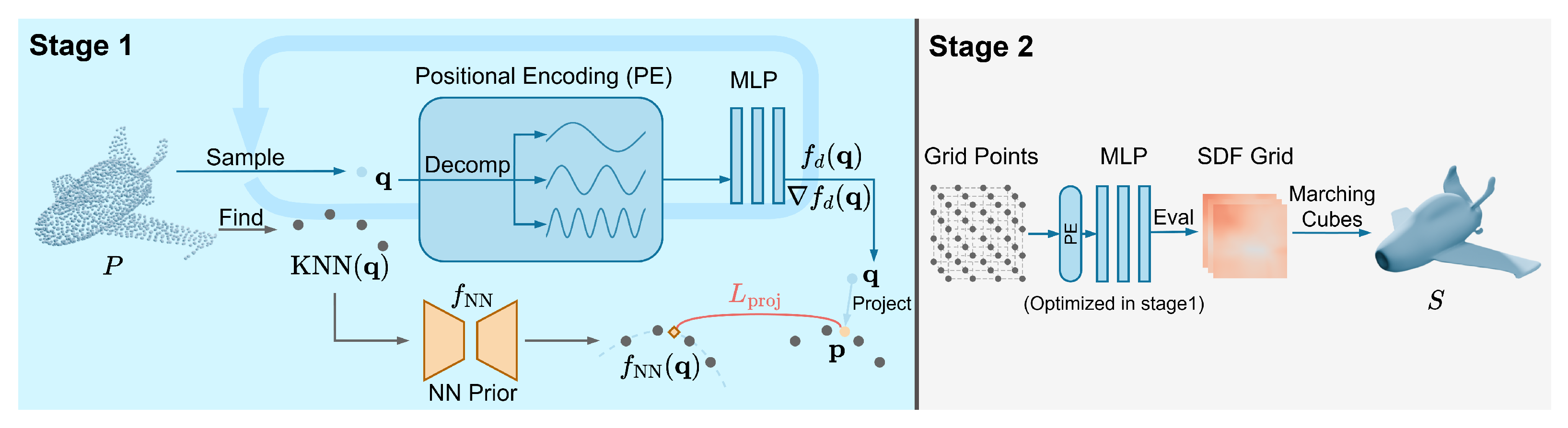
To reconstruct a surface S from a sparse point cloud P, we first optimize the signed distance function $f_d$ to fit the shape of P, then extract its iso-surface to obtain S. Figure 1 illustrates the optimization process (stage 1) and the extraction process (stage 2), where stage 1 is the deterministic stage.

In stage 1, we train $f_d$ to fit the SDF under supervision from a pre-trained data-driven nearest neighbor prior. The signed distance function $f_d$ represented by a neural network will be optimized to minimize a projection loss $L_{\mathrm{proj}}$, which is defined as the distance between the projected point $\mathbf{p}$ derived from $f_d$ and the nearest neighbor ${\mathbf{p}}_{\mathrm{NN}}$ estimated by the prior function $f_{\mathrm{NN}}$. The accuracy of the $f_d$ is reflected by the accuracy of the projection, which is measured by $L_{\mathrm{proj}}$, to achieve normal-free optimization. To encourage the iso-surface of $f_d$ to be more stable and smooth, we add a positional encoding (PE) layer with low-frequency bands in the network representing $f_d$ as regularization.

In stage 2, we uniformly divide the space into voxels and evaluate the SDF value at each grid point using the learned signed distance function $f_d$ in stage 1. Subsequently, we apply the marching cubes algorithm to each voxel for iso-surface extraction to generate the final mesh.

3.3. Nearest Neighbor Prior

The sparsity of point clouds and the lack of point normal information make it impractical to obtain accurate ground truth values of SDFs, which poses significant challenges for direct SDF learning. Therefore, we employ a projection-based optimization approach to optimize the signed distance function. As formulated by Equation (1), a query point $\mathbf{q}$ is projected along the gradient vector $\nabla f_d\left(\gamma \left(\mathbf{q}\right)\right)$ to obtain a projected point $\mathbf{p}$.

$$\mathbf{p}=\mathrm{proj}\left(\mathbf{q}\right)=\mathbf{q}-f_d\left(\gamma \left(\mathbf{q}\right)\right)·{\displaystyle \frac{\nabla f_d\left(\gamma \left(\mathbf{q}\right)\right)}{\parallel \nabla f_d\left(\gamma \left(\mathbf{q}\right)\right)\parallel }}$$

(1)

$\gamma \left(\mathbf{q}\right)$ in Equation (1) denotes the vector obtained by encoding the query point $\mathbf{q}$ through the positional encoding layer (more details are discussed in Section 3.4). Through the comparison between the projected point and the nearest neighbor ${\mathbf{p}}_{\mathrm{NN}}$ predicted by the prior function, we optimize the signed distance function without explicit SDF supervision.

We employ a pre-trained data-driven nearest neighbor prior $f_{\mathrm{NN}}$ to approximate the ground truth value of projection, providing supervision for optimizing $f_d$. Formally, the definition of the nearest neighbor prior function is as follows (Equation (2)): Given a query point $\mathbf{q}$ and its corresponding set $T=\mathrm{KNN}(\mathbf{q},P)$ of K-nearest neighbors in point cloud P, $f_{\mathrm{NN}}$ estimates the nearest neighbor ${\mathbf{p}}_{\mathrm{NN}}$ to the query point $\mathbf{q}$ on the local surface patch determined by T.

$$f_{\mathrm{NN}}(\mathbf{q},T)={\mathbf{p}}_{\mathrm{NN}}$$

(2)

For network implementation, we use a PointNet encoder to extract a geometric feature from the KNN set T, followed by an MLP decoder that regresses the coordinates of ${\mathbf{p}}_{\mathrm{NN}}$. This encoder-decoder network is trained to minimize Euclidean distance between its predicted nearest neighbors and the ground truth values obtained from reference meshes.

The nearest neighbor prior provides supervision during the optimization of the signed distance function $f_d$. Therefore, the accuracy and smoothness properties of the signed distance function are directly influenced by the quality of the prior. While reconstruction tests offer a straightforward way to measure the quality of a prior, such an empirical evaluation suffers from two limitations: (1) high computational costs when performing reconstruction on the whole test set; and (2) inability to decouple errors originating from the optimization process itself. To enable direct quantification of the prediction error of a prior function, we perform some differential analysis on the prediction results.

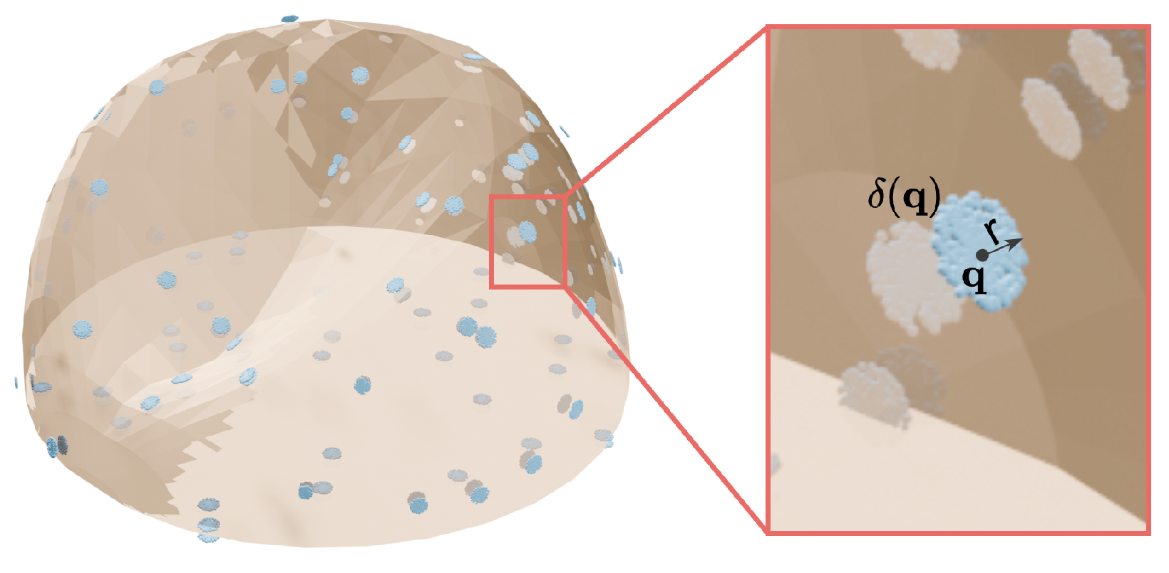
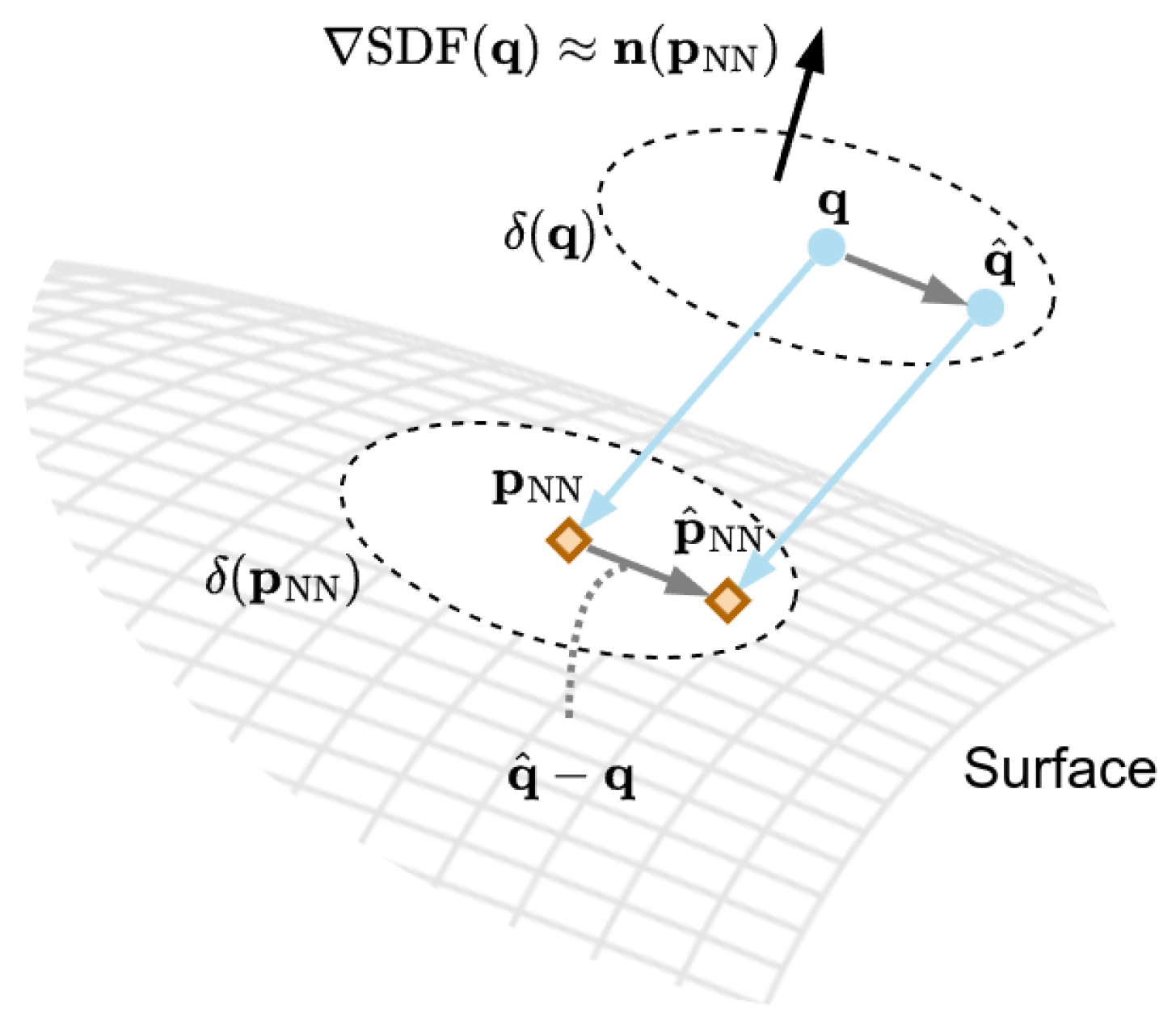
Mathematically, the surface of an object is differentiable almost everywhere, implying that the SDF and its iso-surfaces inherit this differentiable property. We argue the prior function should also maintain similar differentiability, as it supervises $f_d$ to approximate the SDF. To quantify this requirement, we propose a numerical approach for assessing the differentiability of a prior function. As illustrated in Figure 2, given a query point $\mathbf{q}$ and its nearest neighbor ${\mathbf{p}}_{\mathrm{NN}}$ on the surface, the disk neighborhoods $\delta \left(\mathbf{q}\right)$ and $\delta \left({\mathbf{p}}_{\mathrm{NN}}\right)$ should be approximately parallel when their radius becomes sufficiently small. The parallelism enables linear approximation of the nearest neighbor: for any perturbed point $\widehat{\mathbf{q}}\in \delta \left(\mathbf{q}\right)$, the nearest neighbor $f_{\mathrm{NN}}\left(\widehat{\mathbf{q}}\right)$ can be approximated by its first-order Taylor expansion ${\mathbf{p}}_{\mathrm{NN}}+(\widehat{\mathbf{q}}-\mathbf{q})$. The approximation error at $\widehat{\mathbf{q}}$ is $\parallel f_{\mathrm{NN}}\left(\widehat{\mathbf{q}}\right)-({\mathbf{p}}_{\mathrm{NN}}+\widehat{\mathbf{q}}-\mathbf{q}){\parallel }_2$. Larger average approximation error of all $\widehat{\mathbf{q}}\in \delta \left(\mathbf{q}\right)$ indicates less smoothness, because the prior function $f_{\mathrm{NN}}$ is sensitive to small tangential perturbations, thereby suggesting non-differentiability through failure of linear approximation.

To evaluate the average approximation error $E_{\mathrm{tangent}}\left(\mathbf{q}\right)$ over the disk neighborhood $\delta \left(\mathbf{q}\right)$, we sample sufficient perturbed points on it and average the error on each point according to Equation (3) (the KNN set T in Equation (2) is omitted for simplicity):

$$\begin{array}{cc}\hfill E_{\mathrm{tangent}}\left(\mathbf{q}\right)& ={\displaystyle \frac{1}{A\left(\delta \right(\mathbf{q}\left)\right)}}{\int }_{\widehat{\mathbf{q}}\in \delta \left(\mathbf{q}\right)}{∥f_{\mathrm{NN}}\left(\widehat{\mathbf{q}}\right)-({\mathbf{p}}_{\mathrm{NN}}+\widehat{\mathbf{q}}-\mathbf{q})∥}_2\hfill \\ \hfill & \approx {\displaystyle \frac{1}{\left|D\right(\mathbf{q}\left)\right|}}\sum _{\widehat{\mathbf{q}}\in D\left(\mathbf{q}\right)}{∥f_{\mathrm{NN}}\left(\widehat{\mathbf{q}}\right)-({\mathbf{p}}_{\mathrm{NN}}+\widehat{\mathbf{q}}-\mathbf{q})∥}_2\hfill \end{array}$$

(3)

where $A\left(\delta \right(\mathbf{q}\left)\right)$ denotes the area of the disk neighborhood $\delta \left(\mathbf{q}\right)$ and $\left|D\right(\mathbf{q}\left)\right|$ represents the number of sampled points within the $\delta \left(\mathbf{q}\right)$. In practice, we uniformly sample $D\left(\mathbf{q}\right)$ from $\delta \left(\mathbf{q}\right)$, where Figure 3 shows an example of some sets sampled from a beanbag sofa. The distribution of $E_{\mathrm{tangent}}$ of all possible query points around the entire point cloud P reflects the differentiability of a prior function. The more concentrated the $E_{\mathrm{tangent}}$ distribution and the smaller the $E_{\mathrm{tangent}}$ values, the better the differentiability of the prior function. A well-posed prior function should be insensitive to small tangential perturbations. In contrast, an excessive variation would compromise its ability to provide a smooth supervision for $f_d$, potentially inducing some non-differentiable artifacts such as lots of micro spikes.

3.4. Low-Frequency Positional Encoding as a Regularization

The signed distance function $f_d$ may inherit systematic errors from its supervision, as the optimization process minimizes deviations only from the nearest neighbor prior $f_{\mathrm{NN}}$, rather than from the ground truth SDF values. This implies that precise fitting of $f_d$ to $f_{\mathrm{NN}}$ predictions does not strictly equate to proper SDF reconstruction, as any inherent limitations in the prior’s geometric approximation may be propagated to the signed distance function. In practice, $f_d$ may converge to the overall shape of the object quickly, but keep “oscillating” slightly during the following iterations, leading to bubbles or holes in some cases. To address this issue, we introduce a low-frequency positional encoding layer as a regularization for the optimization process (i.e., stage 1 in Figure 1).

The positional encoding (PE) layer serves as a data augmentation strategy integrated into $f_d$ to mitigate the tendency of overfitting $f_{\mathrm{NN}}$. Empirical observations from surfaces reconstructed by existing methods reveal that low-frequency components convey more stable geometric information when the input point cloud is highly sparse. This evidence motivates us to encode the input coordinates with a set of low-frequency sine and cosine functions. In our implementation, the period of each trigonometric function is greater than $1/2$. As the object is scaled to fit into a unit cube, a period greater than $1/2$ means a very low frequency. This effectively reduces high-frequency error inherited from the local prior function.

More specifically, the positional encoding layer tends to fit the low-frequency components. The input coordinates $\mathbf{x}\in {\mathbb{R}}^3$ are transformed into components ${\gamma }_l,{\gamma }_{l+1},\cdots ,{\gamma }_h$ spanning frequencies from $2^l\pi$ to $2^h\pi$. As defined in Equation (4), the final input vector $\gamma \left(\mathbf{x}\right)$ concatenates all components and the original coordinates:

$$\gamma \left(\mathbf{x}\right)=w_l{\gamma }_l\oplus w_{l+1}{\gamma }_{l+1}\oplus \cdots \oplus w_h{\gamma }_h\oplus \mathbf{x}$$

(4)

Here, each ${\gamma }_i$ represents a component at a specific frequency, defined as the concatenation $\sin \left(2^i\pi \mathbf{x}\right)\oplus \cos \left(2^i\pi \mathbf{x}\right)$. $w_i$ denotes the corresponding weight assigned to this frequency component ${\gamma }_i$ (defined as in Equation (5)), which is progressively increased with the intermediate variable $r_i$ influenced by the time-dependent parameter $\alpha$ (as shown in Equations (6) and (7)) [31].

$$w_i=\left(1-\cos \left(\pi r_i\right)\right)/2$$

(5)

$$r_i=\mathrm{clamp}\left(\alpha (h-l+1)-i,0,1\right)$$

(6)

$$\alpha ={\alpha }_0+{\displaystyle \frac{\mathrm{batch}\mathrm{index}}{\mathrm{number}\mathrm{of}\mathrm{batches}}}$$

(7)

Theoretically, $f_d\left(\mathbf{x}\right)$ maintains equivalent approximation capacity to $f_d\left(\gamma \left(\mathbf{x}\right)\right)$ since $\mathbf{x}$ is a part of $\gamma \left(\mathbf{x}\right)$. However, explicit low-frequency components in $\gamma \left(\mathbf{x}\right)$ accelerate convergence to the overall structure during finite optimization iterations. In addition, the frequency spectrum varies temporally through component weights $w_l,w_{l+1},\cdots ,w_h$. The spectral bandwidth expands with increasing $\alpha$, gradually incorporating higher frequency components during optimization. This temporal variation acts as implicit regularization to mitigate overfitting to the prior function.

3.5. Loss Functions for Reconstruction

We design a loss function that quantifies the difference between the signed distance function’s zero iso-surface and the target surface S through sampling. Since neither the zero iso-surface nor the target surface is accessible during optimization, samples on the iso-surface and S are approximated separately. Samples on the signed distance function’s zero iso-surface are obtained by projecting randomly sampled query points according to Equation (1). Samples on S are approximated by a data-driven prior function $f_{\mathrm{NN}}$ that estimates the real nearest neighbor of $\mathbf{q}$ on S. The average Euclidean distance between these samples is the loss function we used.

For a query point $\mathbf{q}$ near the surface, the projected point $\mathbf{p}$ (in Equation (1)) effectively approximates $\mathbf{q}$’s nearest neighbor on the current zero iso-surface. Because $\mathbf{q}$ is near S, we should be able to locate its nearest neighbor on S with a small local surface patch near $\mathbf{q}$, which is determined by the KNN of $\mathbf{q}$ in P. Therefore, we can locate the point on S through $f_{\mathrm{NN}}(\mathbf{q},\mathrm{KNN}(\mathbf{q},P))$. While such local neighborhoods exhibit significant geometric diversity that precludes simple analytical modeling, we observe that recurrent local patterns often transcend object categories. These observations motivate us to design a neural network representing $f_{\mathrm{NN}}$. The projection loss defined in Equation (8) is the average Euclidean distance between projected points and nearest neighbors estimated by $f_{\mathrm{NN}}$, where $\mathrm{proj}\left(\mathbf{q}\right)=\mathbf{p}$ is a projected point computed by Equation (1). To ensure translation invariance, each point within $\mathrm{KNN}(\mathrm{q},P)$ is transformed to $\mathbf{q}$’s local space via Equation (9) for position independence. After this transformation, we can pass only $\mathrm{KNN}(\mathbf{q},P)$ to $f_{\mathrm{NN}}$ because $\mathbf{q}$ is always at the origin.

$$\begin{array}{cc}\hfill L_{\mathrm{proj}}(P,Q)& ={\displaystyle \frac{1}{\left|Q\right|}}\sum _{\mathbf{q}\in Q}\parallel \mathrm{proj}\left(\mathbf{q}\right)-f_{\mathrm{NN}}(\mathbf{q},T){\parallel }_2\hfill \\ \hfill & ={\displaystyle \frac{1}{\left|Q\right|}}\sum _{\mathbf{q}\in Q}\parallel \mathbf{p}-f_{\mathrm{NN}}(\mathbf{q},\mathrm{KNN}(\mathbf{q},P)){\parallel }_2\hfill \end{array}$$

(8)

$$\forall \mathbf{t}\in \mathrm{KNN}(\mathbf{q},P),\mathbf{t}\leftarrow \mathbf{q}-\mathbf{t}$$

(9)

An accurate projection consists of both accurate direction and distance. The nearest neighbor loss in Equation (8) only constrains the product of direction and distance. If only $L_{\mathrm{proj}}$ is applied to $f_d$, it will focus on projecting the query points to the nearest neighbor, not caring about the distance value. The result may be slower convergence or even wrong details of the shape. We resolve this issue by applying Eikonal regularization as Equation (10) to encourage the unit gradient magnitude, which is an intrinsic property of a valid SDF. Our composite loss function defined in Equation (11) balances projection accuracy with Eikonal regularization through ${\lambda }_1$ and ${\lambda }_2$.

$$L_{\mathrm{reg}}\left(Q\right)={\displaystyle \frac{1}{\left|Q\right|}}\sum _{\mathbf{q}\in Q}|{\parallel \nabla f_d\left(\mathbf{q}\right)\parallel }_2-1|$$

(10)

$$L_{\mathrm{total}}={\lambda }_1{L}_{\mathrm{Proj}}+{\lambda }_2{L}_{\mathrm{reg}}$$

(11)

4. Experiments

4.1. Dataset

Point Cloud Dataset We use the seven largest categories from the ShapeNetCore v1 dataset for training and evaluation. For each object, we uniformly sample a point cloud (containing 2048 points) using Poisson Disk Sampling. Each category is then divided into a training set and a test set in a 7:3 ratio. The generated point cloud representation of objects is used for training (or testing) the nearest neighbor prior network and performing reconstruction tests.

To train the nearest neighbor prior network, we sample 8192 query points around each point cloud by adding random offsets from points in it. The offset added to a point follows a normal distribution $N(0,\sigma )$, where $\sigma$ is the distance between the point and its K-th nearest neighbor in the point cloud. The prior network takes $\mathrm{KNN}(\mathbf{q},P)$ (already transformed to $\mathbf{q}$’s local space according to Equation (9)) as input, and is supervised by the distance from $\mathbf{q}$ to the ground truth mesh. We combine and randomly shuffle the input-label pairs from all categories to construct the prior dataset.

Reconstruction Testset In total, we use 700 objects (100 per category) for testing, which are selected from the test set by using the IFPS (Iterative Farthest Point Sampling) algorithm. During each iteration, the algorithm identifies the object that maximizes the sum of Chamfer Distance to all previously unselected objects, thereby selecting representative objects that are distinct from each other.

4.2. Metrics

The reconstructed surface is measured by both accuracy and normal consistency. For accuracy, CD (Chamfer Distance) and F-score are employed. For normal consistency, we adopt the absolute value of the cosine of the angle between the normals of the reconstructed surface and those of the ground truth mesh.

In practice, CD is calculated as the mean Euclidean distance (Equation (12)) of sufficient (300k) sampled points on the reconstructed and ground truth surfaces, where lower values indicate better reconstruction accuracy. The F-score measures the harmonic mean of precision and recall under a distance threshold of 0.001, with higher values (closer to 1.0) reflecting more accurate surface reconstruction.

$$\mathrm{CD}(P_a,P_b)={\displaystyle \frac{1}{2n}}(\sum _{\mathbf{p}\in P_a}\underset{\mathbf{q}\in P_b}{\min }{\parallel \mathbf{p}-\mathbf{q}\parallel }_2+\sum _{\mathbf{p}\in P_b}\underset{\mathbf{q}\in P_a}{\min }{\parallel \mathbf{p}-\mathbf{q}\parallel }_2)$$

(12)

We find that ShapeNetCore v1 does not provide vertex normals, and the calculation of normal vectors is challenging due to geometric constraints. Specifically, a large number of polygonal meshes are non-watertight, non-manifold, and even non-orientable within the dataset. As shown in Figure 4, the mesh faces exhibit inconsistent orientation where the front and back faces are interlaced. Consequently, it is difficult to achieve global consistency of normals by face-flipping operations. We consider that the normal of the same point can be “bidirectional” when calculating the normal consistency. The normal vector of the reconstructed surface is denoted as $\mathbf{n}\left(\mathbf{p}\right)$, and the normal vector of the ground truth mesh is denoted as $\mathbf{n}\left({\mathbf{p}}_{\mathrm{ref}}\right)$. The absolute value of the dot product between $\mathbf{n}\left(\mathbf{p}\right)$ and $\mathbf{n}\left({\mathbf{p}}_{\mathrm{ref}}\right)$ is taken as the cosine similarity while calculating the normal consistency as in Equation (13). Higher normal consistency values indicate better alignment between reconstructed and ground truth surface normals, with a value of 1 representing perfect consistency.

$$\begin{array}{cc}\hfill \mathrm{NC}(S_{\mathrm{recons}},S_{\mathrm{ref}})& \approx {\displaystyle \frac{1}{\left|P_{\mathrm{recons}}\right|}}\sum _{\mathbf{p}\in P_{\mathrm{recons}}}\left|\cos (\mathbf{n}\left(\mathbf{p}\right),\mathbf{n}\left({\mathbf{p}}_{\mathrm{ref}}\right))\right|\hfill \\ \hfill & ={\displaystyle \frac{1}{\left|P_{\mathrm{recons}}\right|}}\sum _{\mathbf{p}\in P_{\mathrm{recons}}}\left|\mathbf{n}\left(\mathbf{p}\right)·\mathbf{n}\left({\mathbf{p}}_{\mathrm{ref}}\right)\right|\hfill \end{array}$$

(13)

4.3. Setup

The hyperparameter settings are as follows. For $f_{\mathrm{NN}}$, the value of K for the KNN is set to 100, the initial learning rate is ${10}^{-4}$, the number of training epochs is 3 (where each epoch implies training with the entire training set once), and the optimizer used is the Cosine Annealing LR Scheduler and Adam Optimizer with a period of 1 epoch and a minimum learning rate of ${10}^{-5}$. The batch size for training $f_{\mathrm{NN}}$ is 4096.

For $f_d$, we set the projection loss weight ${\lambda }_1=100$ and the weight of the Eikonal loss ${\lambda }_2=1$ in Equation (11). Regarding the positional encoding layer, the lower bound parameter l in Equation (5) is −3 (corresponding to a frequency of $2^{-3}\pi$), and the upper bound parameter h is 2 (corresponding to a frequency of $2^2\pi$), and the initialization of the positional encoding weight ${\alpha }_0$ in Equation (7) is 0.3. The initial learning rate is ${10}^{-4}$, the optimizer used is the Adam Optimizer, the batch number for the optimization of $f_d$ is 30,000, and the batch size of the query points during the optimization of $f_d$ is 4096.

4.4. Evaluation and Comparison

We compare our method with three baselines: Neural Pull (NP) [1], On-Surface Prior (OSP) [7], and GeoUDF [8]. Both NP and OSP utilize an optimizable neural network to represent a signed distance function, but OSP employs a data-driven prior function instead of NP’s fixed approximation as its supervision. GeoUDF generates a UDF through a forward pass of its neural network and extracts the iso-surface by solving a global optimization problem.

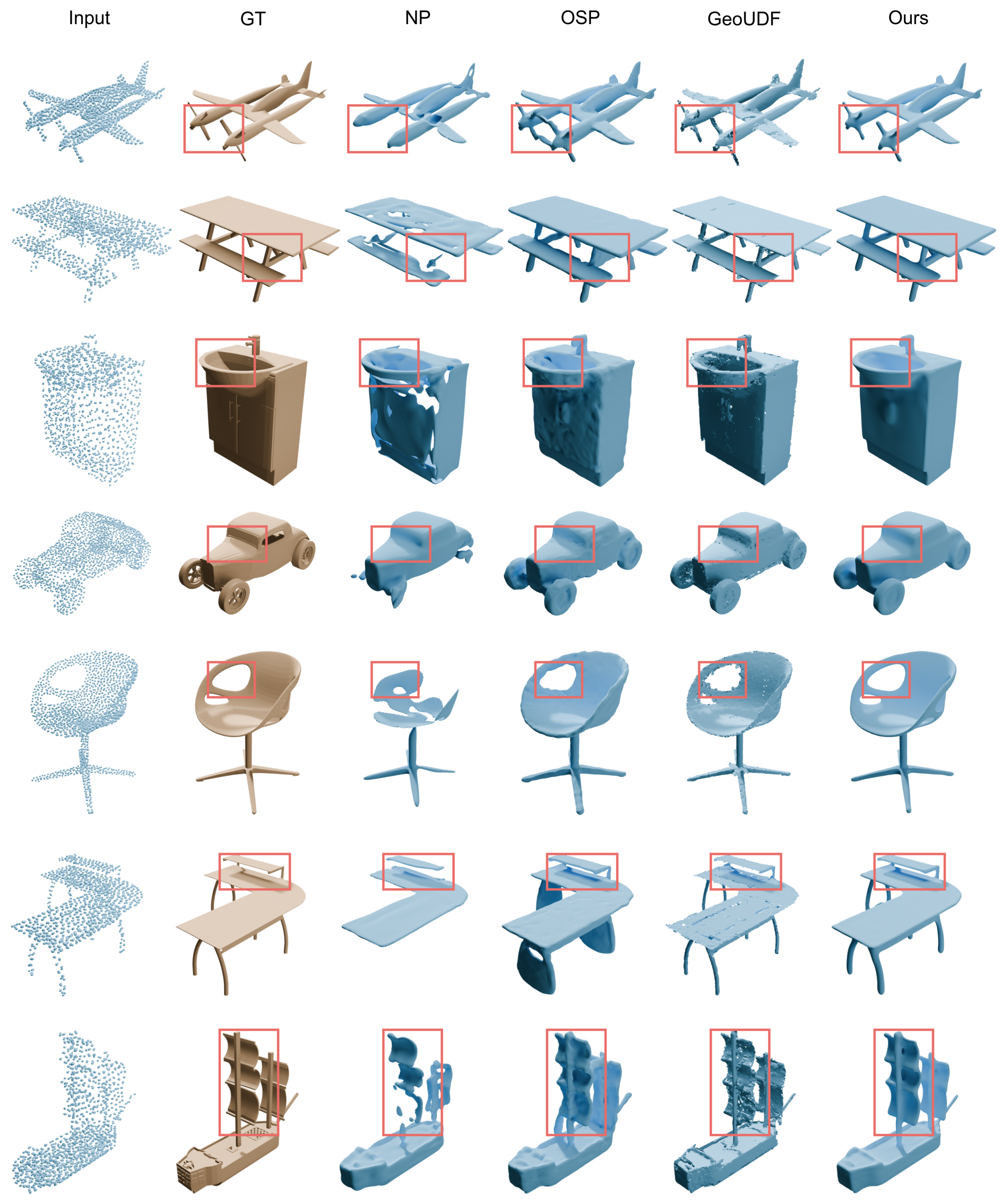
We evaluate all methods on 700 objects mentioned in Section 4.1. For NP, OSP, and our method, we optimize 30k iterations on each point cloud. For NP, 512 query points are sampled in each iteration. For OSP and our method, 4096 query points are sampled. Finally, we extract the 0.003 iso-surface of the signed distance function. We use the official implementation of GeoUDF and keep all configurations unchanged. Quantitative results are shown in Figure 5, in which we can see that our method achieves better accuracy than NP and OSP. In the first row of Figure 5, NP fails to reconstruct the propeller of the airplane, and OSP fuses the two propellers together. Conversely, our method achieves a complete and distinct reconstruction of the airplane propellers. In the second row, concerning the reconstruction of the table, NP leads to the absence of the table legs, and OSP merges the table legs with the tabletop. However, our method reconstructs the table legs with complete and clear structure. In the seventh row, NP loses the mast structure and yields a fragmented sail, while the OSP connects the sail with the hull and generates an uneven sail surface. In contrast, our method maintains the complete structure of the mast and sail as well as the smoothness of the sail surface. From quantitative results in

Table 1. Average CD ($\times {10}^3$).

Category	NP	OSP	Ours	GeoUDF
airplane	8.036	6.722	4.248	1.423
bench	6.560	6.067	4.184	1.600
cabinet	8.165	7.745	5.285	2.237
car	9.594	8.107	6.005	2.809
chair	8.776	6.618	4.253	1.501
table	9.384	6.207	3.987	1.526
vessel	6.494	7.064	4.613	1.535
average	8.144	6.933	4.654	1.804

,

Table 2. Average F-score (with a threshold of 0.001).

Category	NP	OSP	Ours	GeoUDF
airplane	0.960	0.986	0.997	1.000
bench	0.967	0.990	0.994	1.000
cabinet	0.950	0.976	0.990	1.000
car	0.919	0.972	0.989	1.000
chair	0.955	0.985	0.993	1.000
table	0.949	0.991	0.997	1.000
vessel	0.969	0.981	0.992	1.000
average	0.953	0.983	0.993	1.000

and

Table 3. Normal consistency.

Category	NP	OSP	Ours	GeoUDF
airplane	0.905	0.907	0.927	0.905
bench	0.855	0.886	0.910	0.887
cabinet	0.905	0.920	0.946	0.935
car	0.844	0.853	0.868	0.814
chair	0.894	0.906	0.937	0.921
table	0.899	0.925	0.949	0.940
vessel	0.904	0.887	0.911	0.905
average	0.887	0.898	0.921	0.901

, we can also see that our reconstructed surfaces achieve lower CD and higher F-score within each category than NP and OSP.

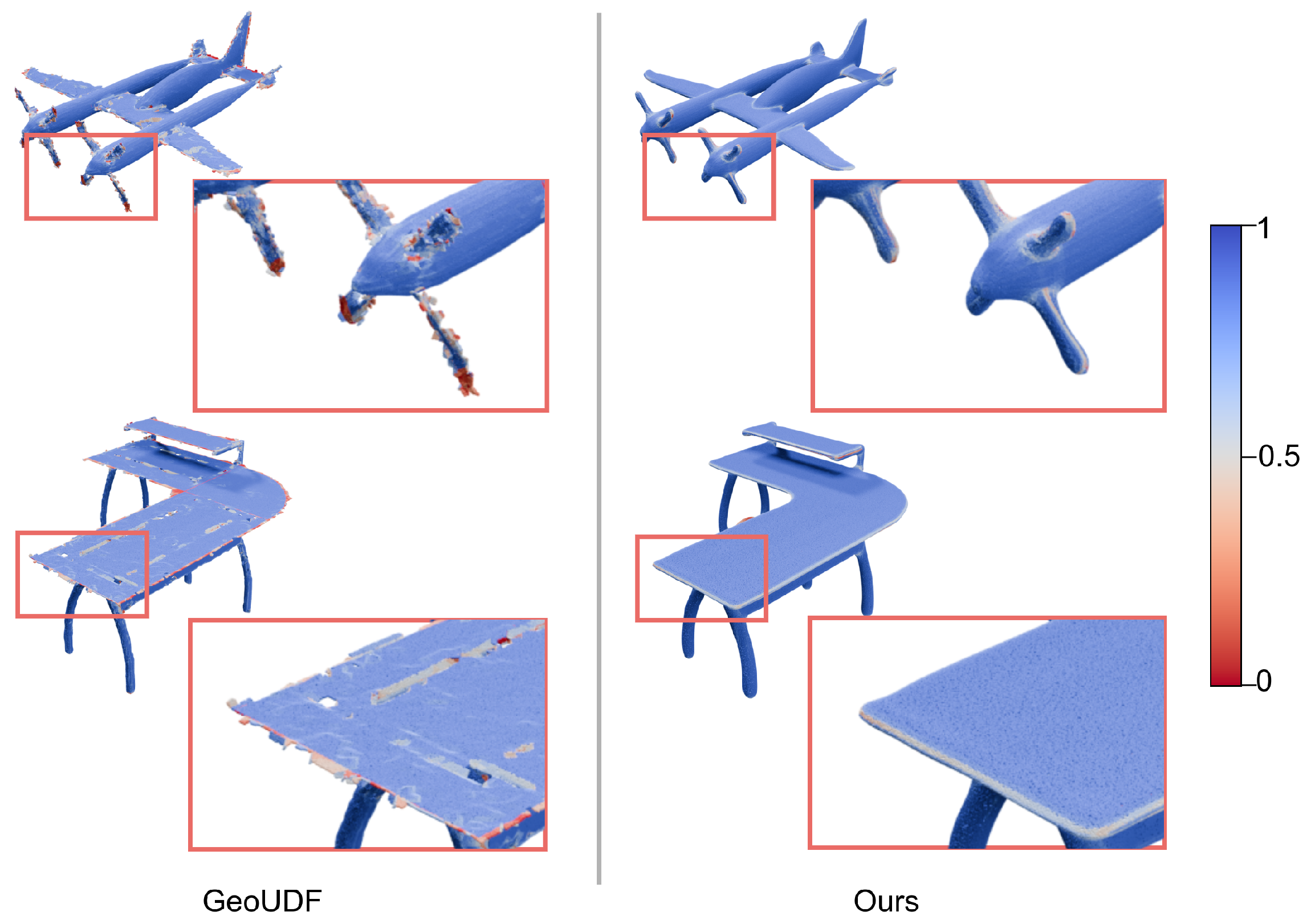
Results demonstrate that although GeoUDF achieves superior accuracy in terms of CD and F-Score metrics compared to our method, it exhibits significantly weaker normal consistency. More precisely, GeoUDF slightly surpasses OSP on NC (0.901 vs. 0.898) but is inferior to our method. This limitation stems from GeoUDF’s use of UDF as an intermediate representation, precluding the application of the marching cubes algorithm to extract surfaces. Although GeoUDF proposes an extraction algorithm approximating marching cubes, this algorithm exhibits inherent flaws that degrade the quality of reconstructed surfaces. To illustrate this issue, we select two generally intact reconstructions produced by GeoUDF (Figure 5) and visualize their normal consistency through color mapping (Figure 6). The results reveal that GeoUDF produces many spikes at edge regions, leading to poor normal consistency in these areas and consequently a lower overall normal consistency. In contrast, our method maintains integrity and smoothness across all regions. Meshes obtained from surface reconstruction are typically used for rendering or subsequent manual modeling. Since both of the processes rely on normals, the defects in the results of GeoUDF affect their usability. In conclusion, GeoUDF achieves high accuracy in reconstruction but lacks practicality. Our method, by employing SDF as the intermediate representation and marching cubes for extraction, ensures that the reconstruction result is a closed manifold.

We also compare our method with the comparative methods in terms of computational and memory requirements as shown in

Table 4. Computational and memory requirements.

Mertic	NP	OSP	GeoUDF	Ours
Runtime (s)	310	662	31	1204
GPU Memory (MiB)	670	880	4910	4346
CPU Memory (MiB)	1063	1086	5895	1700

. We evaluate the four methods by reconstructing the surface of the same object: NP takes 370 s, with a GPU memory usage of 670 MiB and a CPU memory usage of 1063 MiB. OSP requires 662 s, consuming 880 MiB of GPU memory and 1086 MiB of CPU memory. GeoUDF completes in 31 s, while occupying 4910 MiB of GPU memory and 5895 MiB of CPU memory. Our method takes 1204 s, with a GPU memory usage of 4346 MiB and a CPU memory usage of 1700 MiB. Although our method requires the longest time, it achieves superior reconstruction quality, making such a trade-off acceptable.

4.5. Error Analysis and Evaluation of Nearest Neighbor Prior Function

We evaluate the smoothness of different prior functions by analyzing the distribution of the tangent error metric (defined in Equation (3)). Three priors are compared: (1) approximating the nearest neighbor on the surface with the nearest neighbor in the point cloud (employed by NP [1]); (2) predicting the unsigned distance to the surface according to KNN (On-Surface Prior, employed by OSP [7]); (3) predicting the nearest neighbor on the surface according to KNN (our nearest neighbor prior). Since the On-Surface Prior predicts distances rather than points, its error cannot be directly compared with the other two priors. To enable a unified evaluation, the OSP predictions are converted to nearest neighbors according to Equation (14).

$${\mathbf{p}}_{\mathrm{NN}}=\mathbf{q}-f_{\mathrm{OSP}}\left(\mathbf{q}\right)·{\displaystyle \frac{\nabla f_{\mathrm{OSP}}\left(\mathbf{q}\right)}{\parallel \nabla f_{\mathrm{OSP}}\left(\mathbf{q}\right)\parallel }}$$

(14)

To analyze the differentiability of the prior functions, we first sample seed points (denoted as $\mathbf{b}$) on the GT mesh and generate query points by perturbing seed points along their normal vectors (denoted as $\mathbf{n}\left(\mathbf{b}\right)$) with random offsets ranging from −0.001 to 0.001. For each query point $\mathbf{q}$, we establish a local frame $\{\mathbf{n}\left(\mathbf{b}\right),{\mathbf{t}}_1,{\mathbf{t}}_2\}$ using Gram–Schmidt orthogonalization, where ${\mathbf{t}}_1$ and ${\mathbf{t}}_2$ span the tangent plane. Within this tangent plane, we sample 10 points uniformly distributed in a circular region of radius $r_{\delta }={10}^{-3}$ centered at $\mathbf{q}$. These samples constitute a set $D\left(\mathbf{q}\right)$ to approximate the disk neighborhood $\delta \left(\mathbf{q}\right)$ as Equation (3). Finally, we compute the tangent error metric $E_{\mathrm{tangent}}\left(\mathbf{q}\right)$ for each prior function at every query point using this configuration.

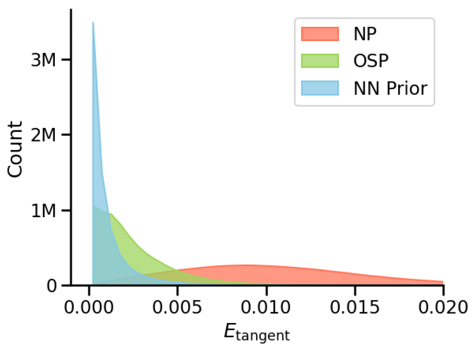
Figure 7 presents the distribution of the tangent error metric for the three prior functions. We analyze the interval [0, 0.02], which encompasses the tangent error values for the majority of query points, by dividing it into uniform sub-intervals of width 5 × 10⁻⁴. The distribution curve of tangent error values is generated by counting the number of query points falling within each sub-interval. The results indicate that our nearest neighbor prior achieves the narrowest error distribution and the lowest error values among the compared methods, suggesting better differential smoothness properties.

4.6. Ablation Study

To validate the effectiveness of the nearest neighbor prior and the positional encoding layer, we conduct ablation studies on the reconstruction test set. The experimental results demonstrate that $f_d$ supervised by the nearest neighbor prior produces more accurate and smoother surfaces, and the PE layer helps to reduce failure cases associated with convergence.

4.6.1. Prior Function

Because $f_d$ always requires supervision, we cannot remove the prior function from the reconstruction pipeline. To validate the effectiveness of our nearest neighbor (NN) prior, we compare it with the On-Surface Prior without using the PE layer.

Table 5. Comparison between nearest neighbor prior and On-Surface Prior.

Metric	NN Prior	On-Surface Prior
CD ($\times {10}^3$)	4.895	6.933
F-Score	0.991	0.983
Normal Consistency	0.913	0.898

shows that the NN prior consistently outperforms the On-Surface Prior across all evaluated metrics.

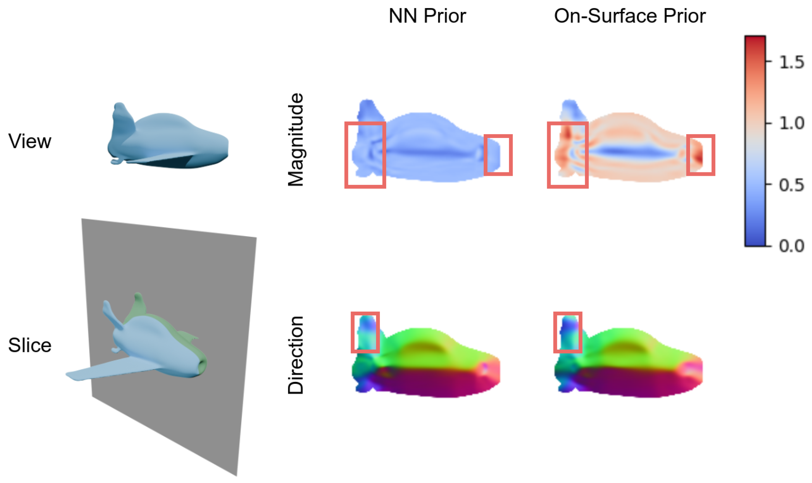
Moreover, a fundamental property of SDF is that its gradient vector at any point is a unit vector. For a signed distance function represented by an MLP, Eikonal regularization constrains the magnitude of the MLP’s gradients. Gradients of $f_d$ on a representative plane are visualized in Figure 8. The visualization reveals that gradients optimized with the On-Surface Prior exhibit more pronounced variations in both magnitude and direction. In comparison, our nearest neighbor prior generates gradients with greater stability and consistency.

4.6.2. Positional Encoding

The low-frequency positional encoding layer and the progressive training strategy serve as a regularization during the optimization process of $f_d$. In this section, we conduct ablation studies on (1) the PE layer, (2) the selection of spectrum, and (3) the choice of the initial value of the progressive parameter $\alpha$.

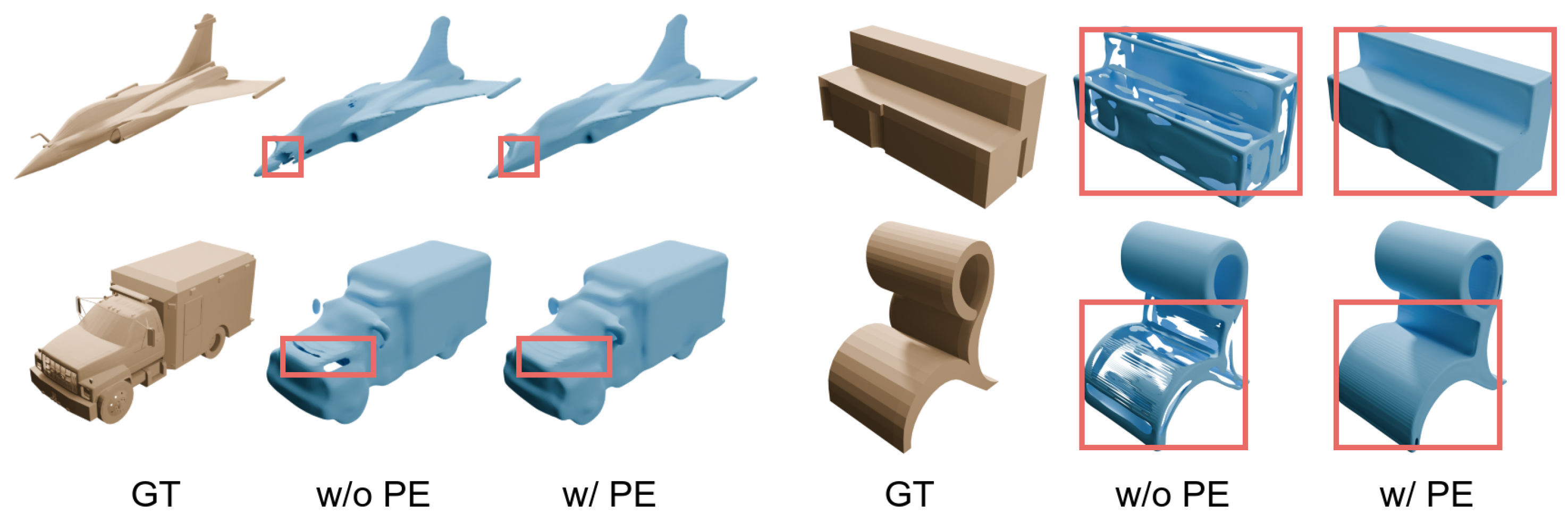
To illustrate how the PE layer affects the optimization process, we remove it from $f_d$ during surface reconstruction.

Table 6. Metrics with/without PE.

Metric	w/PE	w/o PE
CD ($\times {10}^3$)	4.654	4.895
F-Score	0.993	0.991
Normal Consistency	0.921	0.913

shows that removing the PE layer leads to measurable decreases in all metrics. Our analysis of reconstructed surfaces reveals two observations: (1) the PE layer provides no significant improvement for objects that can be reconstructed precisely without PE; (2) it mitigates failure cases associated with convergence. Examples in Figure 9 highlight this behavior: surfaces reconstructed without PE (middle column) exhibit convergence instability, while surfaces reconstructed with PE (right column) maintain structural integrity and stability.

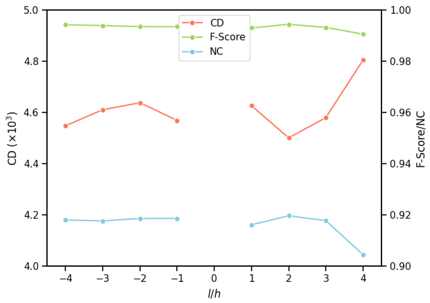
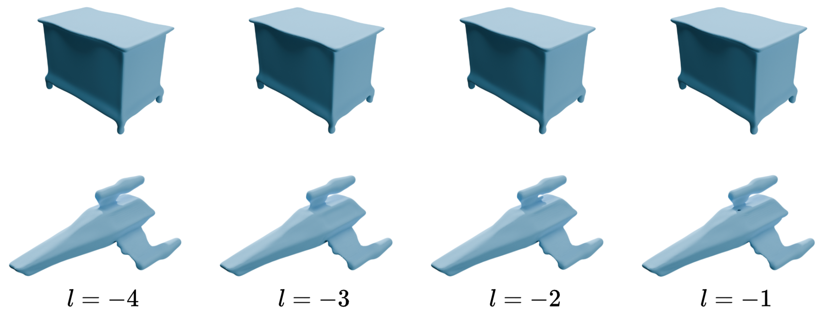
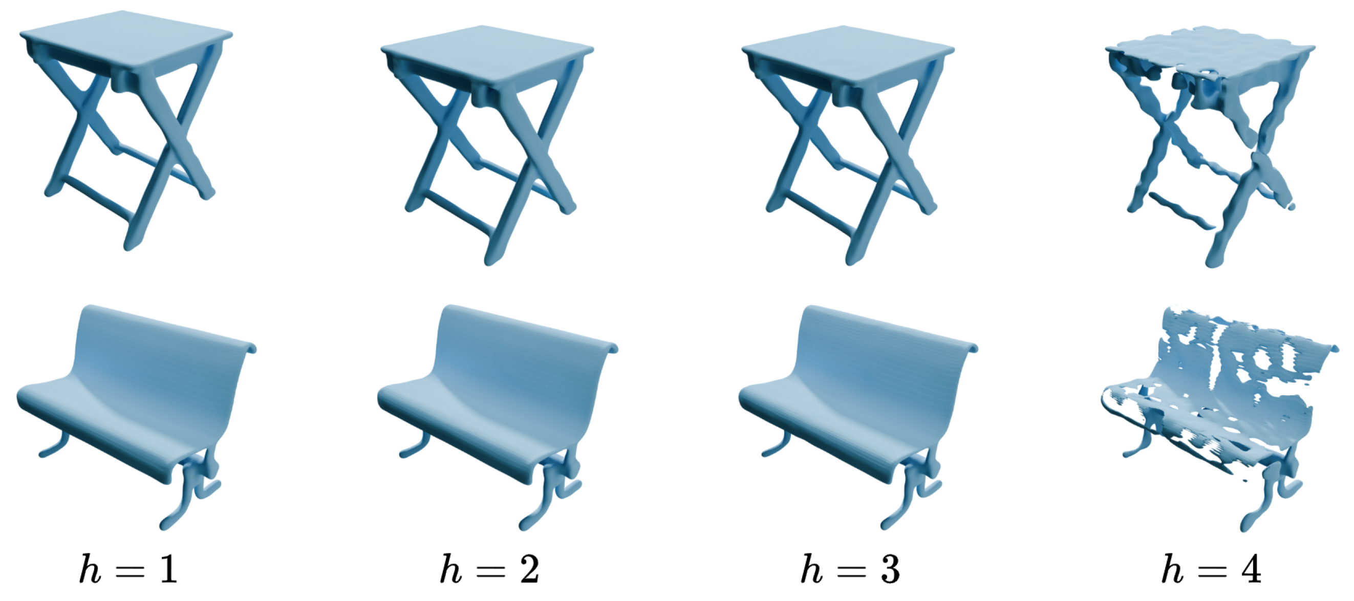
The selected frequency bounds l and h determine the frequency composition in $\gamma \left(\mathbf{x}\right)$, influencing the spectrum that $f_d$ tends to fit during optimization. To evaluate the impact of these spectral range parameters, we conduct ablation studies by either fixing l and varying h or fixing h and varying l from their default values $l=-3$, $h=2$ (corresponding to the spectrum $\{1/8\pi ,1/4\pi ,1/2\pi ,\pi ,2\pi ,4\pi \}$). Figure 10 presents the experiment results. (1) When adjusting the lower bound l within $[-4,-1]$ while maintaining $h=2$, CD shows little variation within this range. A small decrease occurs when lower-frequency components are added, suggesting that incorporating lower-frequency components slightly improves reconstruction accuracy. Meanwhile, both F-score and normal consistency remain nearly unchanged across different l values, indicating that the improvement is limited. Examples shown in Figure 11 support this conclusion. (2) When adjusting the upper bound h within $[1,4]$ (with $l=3$ fixed), the best performance occurs at $h=2$. Notably, introducing the component $h=4$ (corresponding to frequency $16\pi$) leads to significant degradation across all evaluation metrics. This demonstrates that even a relatively high-frequency component may negatively impact the reconstruction result, as evidenced by the examples in Figure 12.

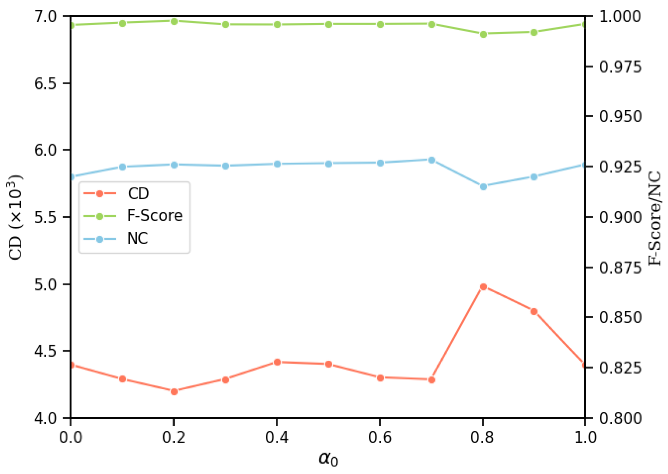
We also validated the rationality of selecting the initial value ${\alpha }_0=0.3$ for the progress parameter $\alpha$, which controls the weight $w_i\in [0,1]$ for each component ${\gamma }_i$. We manually select a representative subset, including 8 distinct objects from each category (56 objects in total) for this ablation study. The results shown in Figure 13 demonstrate that surface quality degrades significantly when ${\alpha }_0>0.7$, with all metrics showing noticeable deterioration. Within the range ${\alpha }_0\in [0,0.7]$, the metrics remain stable with only marginal variations. We set ${\alpha }_0=0.3$ within this stable interval to provide adequate optimization margin for the subsequent progressive increase of $\alpha$.

4.6.3. Rotation Invariance

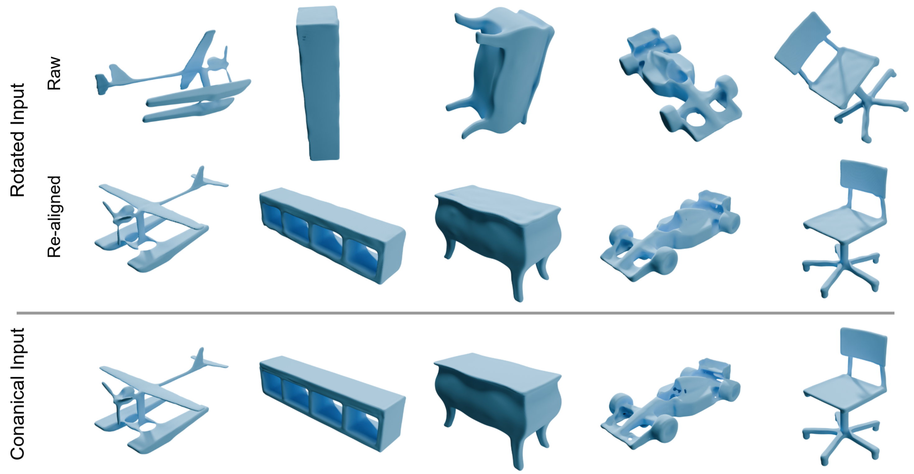
Our method possesses the property of rotation invariance. We evaluate this property using the same dataset employed in the ${\alpha }_0$ ablation study. By applying a random rotation transformation to the input point cloud before reconstruction, we obtained the comparative metrics (compared with the ${\alpha }_0=0.3$ ablation study) presented in

Table 7. Metrics with/without rotation.

Metric	Rotated Input	Canonical Input
CD ($\times {10}^3$)	4.658	4.291
F-Score	0.995	0.996
Normal Consistency	0.913	0.926

. Performing marching cubes in an oblique view causes more aliasing than in a canonical view, and this leads to stair-step artifacts on the reconstructed surface. Therefore, the reconstructed results obtained after rotating will have higher CD values and lower F-score and normal consistency values. However, even with rotation, CD, F-score, and normal consistency exhibit only marginal changes. This minimal performance degradation confirms that our method maintains satisfactory reconstruction accuracy under arbitrary rotations, with all metrics remaining within acceptable tolerance thresholds. Some examples shown in Figure 14 also illustrate that the precision and smoothness of reconstructed surfaces are not obviously affected by rotation of the input.

4.7. Application

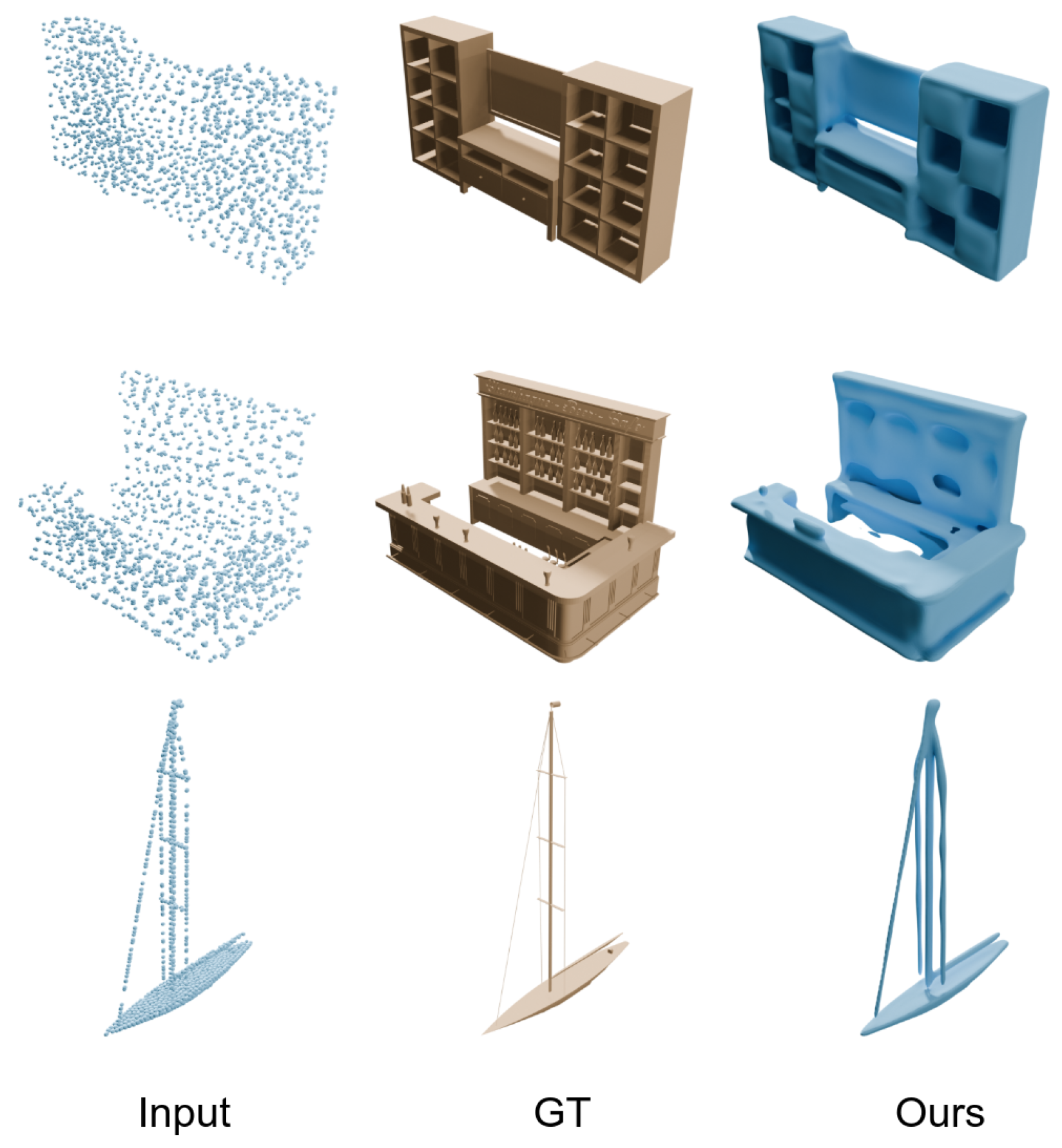
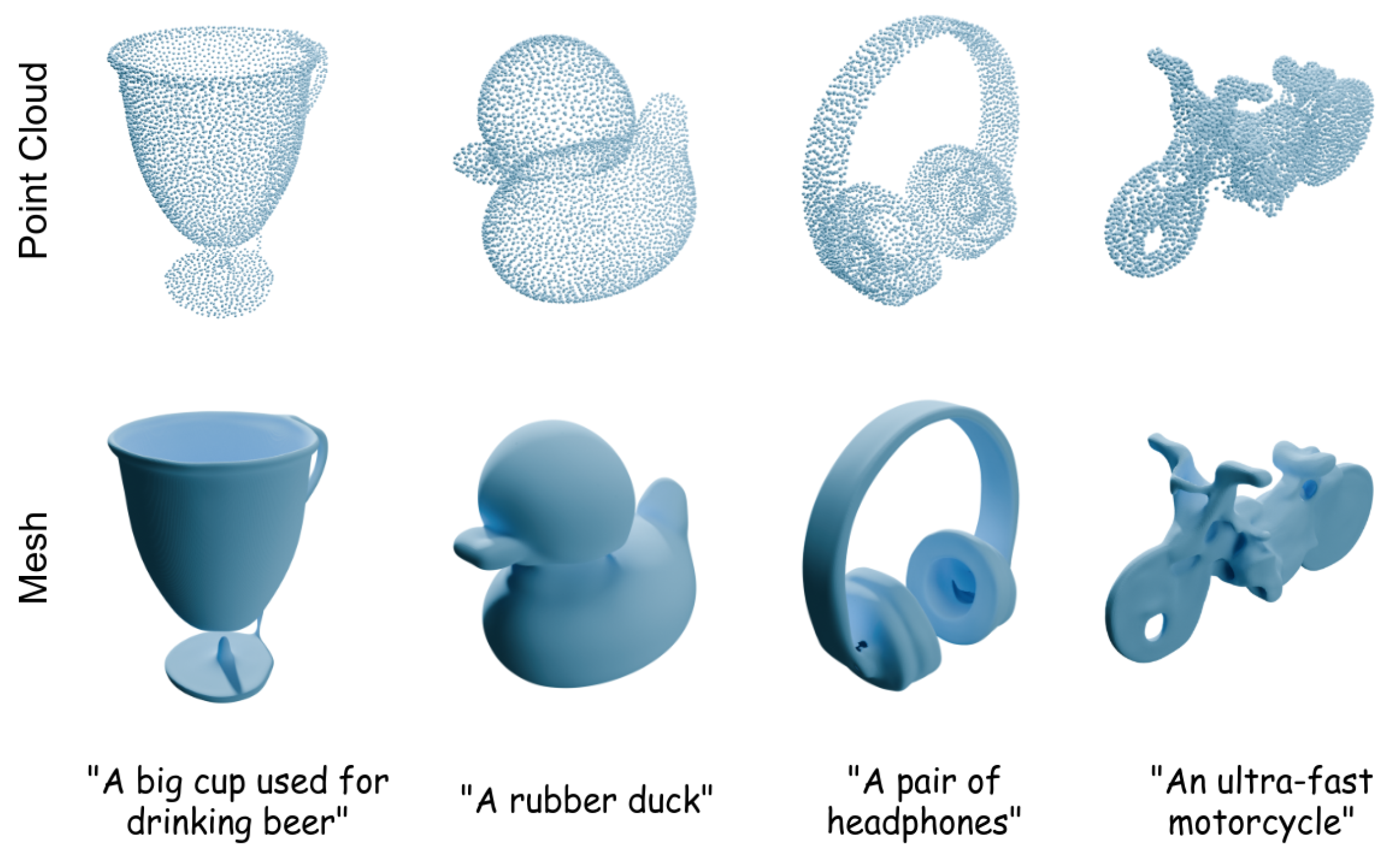
To explore a possible way for achieving 3D generation, we utilize the Point-E [32] (a point cloud generation model) to generate point clouds, then reconstruct the surface. Point-E can generate point clouds with a density of 4096 points. Figure 15 presents surface reconstruction results obtained by first guiding Point-E with text prompts to generate point clouds, followed by processing through our method. All these results are outside the seven object categories used in this paper and lack corresponding reference results. However, our method can still reconstruct complete and accurate surface. Experimental tests indicate that our method needs about 4 GiB of GPU memory and can finish surface reconstruction with just a single RTX 2060 GPU at the least. Therefore, combining a higher-quality point cloud generation model with our surface reconstruction method offers a way to explore the possibility of a low-cost 3D generation pipeline.

5. Conclusions and Discussion

In this paper, we introduce a novel surface reconstruction method for sparse point clouds. Our method can reconstruct smooth, watertight surfaces robustly against sparsity and diversity. The experiments demonstrate the effectiveness of our nearest neighbor prior and the low-frequency positional encoding layer.

Our method sometimes fails to precisely reconstruct shapes with many concave or thin structures, such as a cabinet with many storage units or a vessel with a long, thin mast (as shown in Figure 16). For regular, concave structures like storage units, the current density of query points may not be sufficient to make the MLP converge well. For the thin structures, our nearest neighbor prior may provide inaccurate nearest neighbors, resulting in missing details in the reconstructed shape. We plan to design a non-uniform sampling method or an auxiliary loss to enhance the quality of such local areas while preserving the overall structure. On the other hand, as an optimization-based method, we also have to balance between time and quality. Therefore, improving the efficiency of our method through a well-designed optimization process is also valuable.

References

1. Ma, B.; Han, Z.; Liu, Y.S.; Zwicker, M. Neural-Pull: Learning Signed Distance Function from Point clouds by Learning to Pull Space onto Surface. In Proceedings of the 38th International Conference on Machine Learning; Meila, M., Zhang, T., Eds.; PMLR: Cambridge, MA, USA, 2021; Volume 139, pp. 7246–7257. [Google Scholar]
2. Kazhdan, M.; Hoppe, H. Screened poisson surface reconstruction. ACM Trans. Graph. ToG 2013, 32, 29. [Google Scholar] [CrossRef]
3. Williams, F.; Schneider, T.; Silva, C.; Zorin, D.; Bruna, J.; Panozzo, D. Deep geometric prior for surface reconstruction. In 2019 IEEE/CVF Conference on Computer Vision and Pattern Recognition (CVPR); IEEE: Piscataway, NJ, USA, 2019; pp. 10130–10139. [Google Scholar]
4. Gadelha, M.; Wang, R.; Maji, S. Deep manifold prior. In 2021 IEEE/CVF International Conference on Computer Vision Workshops (ICCVW); IEEE: Piscataway, NJ, USA, 2021; pp. 1107–1116. [Google Scholar]
5. Yuan, G.; Fu, Q.; Mi, Z.; Luo, Y.; Tao, W. SSRNet: Scalable 3D Surface Reconstruction Network. IEEE Trans. Vis. Comput. Graph. 2023, 29, 4906–4919. [Google Scholar] [CrossRef] [PubMed]
6. Tretschk, E.; Tewari, A.; Golyanik, V.; Zollhöfer, M.; Stoll, C.; Theobalt, C. Patchnets: Patch-based generalizable deep implicit 3D shape representations. In Computer Vision—ECCV 2020; Springer: Cham, Switzerland, 2020; pp. 293–309. [Google Scholar]
7. Ma, B.; Liu, Y.S.; Han, Z. Reconstructing surfaces for sparse point clouds with on-surface priors. In 2022 IEEE/CVF Conference on Computer Vision and Pattern Recognition (CVPR); IEEE: Piscataway, NJ, USA, 2022; pp. 6315–6325. [Google Scholar]
8. Ren, S.; Hou, J.; Chen, X.; He, Y.; Wang, W. Geoudf: Surface reconstruction from 3d point clouds via geometry-guided distance representation. In 2023 IEEE/CVF International Conference on Computer Vision (ICCV); IEEE: Piscataway, NJ, USA, 2023; pp. 14214–14224. [Google Scholar]
9. Tian, H.; Zhu, C.; Shi, Y.; Xu, K. SuperUDF: Self-supervised UDF Estimation for Surface Reconstruction. IEEE Trans. Vis. Comput. Graph. 2023, 30, 5965–5975. [Google Scholar] [CrossRef] [PubMed]
10. Botsch, M.; Kobbelt, L.; Pauly, M.; Alliez, P.; Lévy, B. Polygon Mesh Processing; CRC Press: Boca Raton, FL, USA, 2010. [Google Scholar]
11. Huang, Z.; Wen, Y.; Wang, Z.; Ren, J.; Jia, K. Surface Reconstruction from Point Clouds: A Survey and a Benchmark. IEEE Trans. Pattern Anal. Mach. Intell. 2024, 46, 9727–9748. [Google Scholar] [CrossRef] [PubMed]
12. Amenta, N.; Bern, M.; Kamvysselis, M. A new Voronoi-based surface reconstruction algorithm. In SIGGRAPH98: The 25th International Conference on Computer Graphics and Interactive Techniques; Association for Computing Machinery: New York, NY, USA, 1998; pp. 415–421. [Google Scholar] [CrossRef]
13. Barhak, J.; Fischer, A. Parameterization and reconstruction from 3D scattered points based on neural network and PDE techniques. IEEE Trans. Vis. Comput. Graph. 2001, 7, 1–16. [Google Scholar] [CrossRef]
14. Kazhdan, M.; Bolitho, M.; Hoppe, H. Poisson surface reconstruction. In Proceedings of the Fourth Eurographics Symposium on Geometry Processing; Eurographics Association: Goslar, Germany, 2006; pp. 61–70. [Google Scholar]
15. Schnabel, R.; Wahl, R.; Klein, R. Efficient RANSAC for Point-Cloud Shape Detection. Comput. Graph. Forum 2007, 26, 214–226. [Google Scholar] [CrossRef]
16. Nan, L.; Wonka, P. Polyfit: Polygonal surface reconstruction from point clouds. In 2017 IEEE International Conference on Computer Vision (ICCV); IEEE: Piscataway, NJ, USA, 2017; pp. 2353–2361. [Google Scholar]
17. Atzmon, M.; Haim, N.; Yariv, L.; Israelov, O.; Maron, H.; Lipman, Y. Controlling neural level sets. Adv. Neural Inf. Process. Syst. 2019, 32, 182. [Google Scholar]
18. Hanocka, R.; Metzer, G.; Giryes, R.; Cohen-Or, D. Point2Mesh: A self-prior for deformable meshes. ACM Trans. Graph. 2020, 39, 126. [Google Scholar] [CrossRef]
19. Zhao, W.; Lei, J.; Wen, Y.; Zhang, J.; Jia, K. Sign-agnostic implicit learning of surface self-similarities for shape modeling and reconstruction from raw point clouds. In 2021 IEEE/CVF Conference on Computer Vision and Pattern Recognition (CVPR); IEEE: Piscataway, NJ, USA, 2021; pp. 10256–10265. [Google Scholar]
20. Liao, Y.; Donne, S.; Geiger, A. Deep marching cubes: Learning explicit surface representations. In 2018 IEEE/CVF Conference on Computer Vision and Pattern Recognition; IEEE: Piscataway, NJ, USA, 2018; pp. 2916–2925. [Google Scholar]
21. Mescheder, L.; Oechsle, M.; Niemeyer, M.; Nowozin, S.; Geiger, A. Occupancy networks: Learning 3D reconstruction in function space. In 2019 IEEE/CVF Conference on Computer Vision and Pattern Recognition (CVPR); IEEE: Piscataway, NJ, USA, 2019; pp. 4460–4470. [Google Scholar]
22. Park, J.J.; Florence, P.; Straub, J.; Newcombe, R.; Lovegrove, S. Deepsdf: Learning continuous signed distance functions for shape representation. In 2019 IEEE/CVF Conference on Computer Vision and Pattern Recognition (CVPR); IEEE: Piscataway, NJ, USA, 2019; pp. 165–174. [Google Scholar]
23. Badki, A.; Gallo, O.; Kautz, J.; Sen, P. Meshlet priors for 3D mesh reconstruction. In 2020 IEEE/CVF Conference on Computer Vision and Pattern Recognition (CVPR); IEEE: Piscataway, NJ, USA, 2020; pp. 2849–2858. [Google Scholar]
24. Chibane, J.; Alldieck, T.; Pons-Moll, G. Implicit functions in feature space for 3D shape reconstruction and completion. In 2020 IEEE/CVF Conference on Computer Vision and Pattern Recognition (CVPR); IEEE: Piscataway, NJ, USA, 2020; pp. 6970–6981. [Google Scholar]
25. Peng, S.; Niemeyer, M.; Mescheder, L.; Pollefeys, M.; Geiger, A. Convolutional occupancy networks. In Computer Vision—ECCV 2020; Springer: Cham, Switzerland, 2020; pp. 523–540. [Google Scholar]
26. Huang, J.; Gojcic, Z.; Atzmon, M.; Litany, O.; Fidler, S.; Williams, F. Neural kernel surface reconstruction. In 2023 IEEE/CVF Conference on Computer Vision and Pattern Recognition (CVPR); IEEE: Piscataway, NJ, USA, 2023; pp. 4369–4379. [Google Scholar]
27. Sitzmann, V.; Martel, J.N.P.; Bergman, A.W.; Lindell, D.B.; Wetzstein, G. Implicit neural representations with periodic activation functions. In Proceedings of the 34th International Conference on Neural Information Processing Systems; Curran Associates Inc.: Red Hook, NY, USA, 2020. [Google Scholar]
28. Yifan, W.; Rahmann, L.; Sorkine-hornung, O. Geometry-Consistent Neural Shape Representation with Implicit Displacement Fields. In Proceedings of the Tenth International Conference on Learning Representations, Virtual, 25 April 2022. [Google Scholar]
29. Wang, P.; Liu, L.; Liu, Y.; Theobalt, C.; Komura, T.; Wang, W. NeuS: Learning neural implicit surfaces by volume rendering for multi-view reconstruction. In Proceedings of the 35th International Conference on Neural Information Processing Systems; Curran Associates Inc.: Red Hook, NY, USA, 2021. [Google Scholar]
30. Mildenhall, B.; Srinivasan, P.P.; Tancik, M.; Barron, J.T.; Ramamoorthi, R.; Ng, R. NeRF: Representing scenes as neural radiance fields for view synthesis. Commun. ACM 2021, 65, 99–106. [Google Scholar] [CrossRef]
31. Wang, Y.; Skorokhodov, I.; Wonka, P. HF-NeuS: Improved Surface Reconstruction Using High-Frequency Details. Adv. Neural Inf. Process. Syst. 2022, 35, 1966–1978. [Google Scholar]
32. Nichol, A.; Jun, H.; Dhariwal, P.; Mishkin, P.; Chen, M. Point-E: A System for Generating 3D Point Clouds from Complex Prompts. arXiv 2022, arXiv:2212.08751. [Google Scholar] [CrossRef]
Figure 1. The reconstruction pipeline. In stage 1, the MLP is optimized to minimize L NN (described in Equation (8)). The left part illustrates an iteration of the optimization process. After optimization, the MLP fits the shape of P. In stage 2, we evaluate the MLP at grid points to obtain an SDF grid and run marching cubes to extract a surface.
Applsci 16 01210 g001
Figure 2. Illustration of nearest neighbor approximation in the disk neighborhood. A query point q and its surface nearest neighbor p NN have disk neighborhoods δ ( q ) and δ ( p NN ) (dashed). The arrow q ^ q shows a small perturbation of q within δ ( q ) . p NN + ( q ^ q ) gives the approximation of the nearest neighbor of q ^ .
Applsci 16 01210 g002
Figure 3. Disk neighborhoods sampled to compute E tangent for a beanbag sofa. The surface is rendered with transparency to show the neighborhoods inside. For clarity, the radius of a neighborhood (r) is scaled to 10 times the actual value used in our computations.
Applsci 16 01210 g003
Figure 4. Examples of objects with disordered patch orientations in the ShapeNetCore dataset. (Blue represents the front faces, red represents the back faces. The results are rendered with Blender (Blender Foundation, Amsterdam, The Netherlands) version [4.5]).
Applsci 16 01210 g004
Figure 5. Comparison between NP [1], OSP [7], GeoUDF [8], and our method.
Applsci 16 01210 g005
Figure 6. Some defects (small holes and burrs) on the surfaces reconstructed by GeoUDF, where colors vary continuously from blue (high normal consistency, values near 1) to red (low normal consistency, values near 0).
Applsci 16 01210 g006
Figure 7. Distribution of tangent error. We plot this distribution curve with bin width 5 × 10⁻⁴. Our nearest neighbor prior has the lowest tangent error and the most concentrated error distribution.
Applsci 16 01210 g007
Figure 8. Gradient of f d optimized with nearest neighbor prior (left) and On-Surface Prior (right) at the z = 0.0176 plane. Because the query points are only sampled around the input point cloud, the rest of the unit cube is masked.
Applsci 16 01210 g008
Figure 9. Comparison between surface reconstructed with PE and without PE.
Applsci 16 01210 g009
Figure 10. Effect of frequency range selection on reconstruction (left: keeping h = 2 constant while varying parameter l; right: keeping l = 3 constant while modifying h).
Applsci 16 01210 g010
Figure 11. Reconstructed surfaces with different l values ( h = 2 fixed). There is no significant difference in the rendered results.
Applsci 16 01210 g011
Figure 12. Reconstructed surfaces with different h values ( l = 3 fixed). Degeneration can be observed when h = 4 .
Applsci 16 01210 g012
Figure 13. Effect of initial value for the optimization schedule parameter ( α 0 ) on reconstruction.
Applsci 16 01210 g013
Figure 14. Surfaces reconstructed from randomly rotated point clouds. The first row shows surfaces reconstructed from rotated input, the second row shows the same surfaces but re-aligned (rotated back) to the canonical view, and the third row shows surfaces reconstructed directly from the canonical input.
Applsci 16 01210 g014
Figure 15. Point cloud generated by Point-E (the upper row) and the reconstructed surfaces (the lower row).
Applsci 16 01210 g015
Figure 16. Some failure cases.
Applsci 16 01210 g016