


Abstract
Pollen identification is critical for melissopalynology (honey authentication), ecological monitoring, and allergen tracking, yet manual microscopic analysis remains labor-intensive, subjective, and error-prone when multiple grains overlap in realistic samples. Existing automated approaches often fail to address multi-grain scenarios or lack systematic comparison across classical and deep learning paradigms, limiting their practical deployment. This study proposes a subinstance-based classification framework combining YOLOv12n object detection for grain isolation, independent classification via classical machine learning (ML), convolutional neural networks (CNNs), or Vision Transformers (ViTs), and majority voting aggregation. Five classical classifiers with systematic feature selection, three CNN architectures (ResNet50, EfficientNet-B0, ConvNeXt-Tiny), and three ViT variants (ViT-B/16, ViT-B/32, ViT-L/16) are evaluated on four datasets (full images vs. isolated grains; raw vs. CLAHE-preprocessed) for four berry pollen species (Ribes nigrum, Ribes uva-crispa, Lonicera caerulea, and Amelanchier alnifolia). Stratified image-level splits ensure no data leakage, and explainable AI techniques (SHAP, Grad-CAM++, and gradient saliency) validate biological interpretability across all paradigms. Results demonstrate that grain isolation substantially improves classical ML performance (F1 from 0.83 to 0.91 on full images to 0.96–0.99 on isolated grains, +8–13 percentage points), while deep learning excels on both levels (CNNs: F1 = 1.000 on full images with CLAHE; ViTs: F1 = 0.99). At the instance level, all paradigms converge to near-perfect discrimination (F1 ≥ 0.96), indicating sufficient capture of morphological information. Majority voting aggregation provides +3–5% gains for classical methods but only +0.3–4.8% for deep models already near saturation. Explainable AI analysis confirms that models rely on biologically meaningful cues: blue channel moments and texture features for classical ML (SHAP), grain boundaries and exine ornamentation for CNNs (Grad-CAM++), and distributed attention across grain structures for ViTs (gradient saliency). Qualitative validation on 211 mixed-pollen images confirms robust generalization to realistic multi-species samples. The proposed framework (YOLOv12n + SVC/ResNet50 + majority voting) is practical for deployment in honey authentication, ecological surveys, and fine-grained biological image analysis.
1. Introduction
Pollen identification plays an important role in ecology, agriculture, and food quality control. In melissopalynology, microscopic examination of pollen grains remains the primary method for verifying the botanical origin of honey. This process is notoriously labor-intensive, time-consuming, and prone to human error, especially when analysts face large sample volumes or must distinguish morphologically similar taxa [1]. The growing demand for high-throughput analysis—across real-time allergen monitoring, large-scale biodiversity surveys, and routine honey authentication—has intensified the need for automated, objective, and scalable systems for pollen identification [2]. Automated image-based classification supported by machine learning offers a promising direction to reduce manual workload and improve reproducibility.
Traditional melissopalynology, established by Pfister in 1895, has been the gold standard for determining both the botanical and geographical origin of honey for well over a century [3]. Analysts identify and count pollen grains to confirm monofloral honey labels and detect adulteration, but this expert-driven process is slow, costly, and depends on a small number of specialists. Identification is often slow, tedious, and to some extent subjective, particularly when differentiating species with very similar morphologies [1]. For instance, pollen from Rubus fruticosus (blackberry) and Rubus idaeus (raspberry) is difficult to distinguish under the microscope, yet these plants grow in different ecological conditions, making precise identification relevant for determining geographical origin [4]. Because of these challenges, inconsistencies may arise between analysts, or even within the work of the same analyst over time.
Various molecular and spectroscopic techniques have been proposed as alternatives or complements to microscopy, including DNA metabarcoding, Fourier transform infrared spectroscopy, and mass-spectrometry-based chemometrics [5], while these methods offer higher taxonomic resolution or improved automation, they also introduce new limitations, such as high operating costs, lack of quantitative information (e.g., for DNA metabarcoding) and dependence on large reference databases [6]. Thus, there remains a strong need for methods that preserve the morphological interpretability of microscopy but incorporate the speed and objectivity of automated analysis.
Automated pollen classification from microscopic images introduces its own technical challenges. Pollen grains vary in appearance depending on their orientation, level of focus, illumination, preservation state, and degree of clustering with neighboring grains [1]. Additional image artifacts, such as dust, background structures, or out-of-focus regions, can further degrade classification performance [7]. A successful automated system must therefore learn stable, species-specific morphological cues while remaining robust to noise and natural variation. A related difficulty is the need for high-quality annotated datasets, ideally containing hundreds or thousands of well-labeled images per pollen type [2]. Such datasets are costly to produce and are often incomplete, making the development of robust models even more challenging.
Pollen grains themselves carry important biological and ecological information. As the male gametophytes of seed plants, they enable fertilization by transporting genetic material from one flower to another. Their durable outer wall, the exine, makes pollen highly resistant to decay, allowing grains to persist in soil, sediments, and honey [8]. For these reasons, palynology provides valuable insights into plant distribution, climate history, and ecological interactions. Automated identification systems stand to greatly enhance this work by enabling rapid analysis of large datasets that would not be feasible using manual inspection.
The following four pollen types from economically and ecologically important berry-producing shrubs were selected for this study: blackcurrant (Ribes nigrum), gooseberry (Ribes uva-crispa), haskapberry (Lonicera caerulea L. var. kamtschatica Sevast.), and serviceberry (Amelanchier alnifolia Nutt.). These genera are characterized by distinctive but fine-grained morphological differences. Capture of such subtle geometric and textural cues—often visible only when grains are optimally oriented—remains a central difficulty for automated systems. Nevertheless, accurate identification of these species is critical not only for ecological studies but also for the food industry, as these plants contribute to high-value monofloral honeys and berry-derived bee products.
The primary novelty is a subinstance-based classification framework: images are decomposed into individual pollen grains via YOLOv12n detection, classified independently, then aggregated via majority voting. This instance-level approach yields better discrimination and reduces confounding effects from background artifacts compared to whole-image classification, while maintaining interpretability through explicit grain boundaries and enabling direct quantification of pollen composition in mixed samples, essential for honey authentication. The objective of this research is to evaluate how whole-image and instance-level classification workflows perform across classical and deep learning methods, and to determine which combination yields the highest accuracy and robustness for fine-grained berry pollen identification. Performance improvements through the integration of object detection with classification are demonstrated, providing a practical pathway toward real-world applications in honey authentication, ecological monitoring, and automated palynology. To further validate practical applicability, the trained models were qualitatively assessed on an additional dataset of 211 mixed-pollen images containing multiple species per field, confirming that the YOLOv12n detector successfully segments individual grains for independent classification without requiring majority voting aggregation.
Beyond quantitative performance metrics, understanding how and why predictions are made by models is critical for building trust and enabling scientific insight. Therefore, explainable artificial intelligence (XAI) techniques were employed to interpret model decisions across all three paradigms as follows: SHAP (SHapley Additive exPlanations) analysis for classical feature-based models, Grad-CAM++ for CNNs, and gradient-based attention visualization for Vision Transformers. These complementary interpretability methods reveal which morphological features, spatial regions, or image patches drive classification, providing validation that biologically meaningful patterns rather than spurious correlations are learned by models.
1.1. Research Problems and Challenges
Despite the progress in automated pollen classification, several critical challenges remain unresolved in the literature. First, multi-grain and cluttered samples. Most existing datasets and methods focus on isolated, well-prepared single-grain images, ignoring the reality of honey and environmental samples where multiple overlapping grains, debris, and background artifacts coexist [9,10,11]. Second, fine-grained species discrimination. Distinguishing morphologically similar pollen taxa (e.g., closely related berry species) requires capturing subtle textural and geometric cues that are sensitive to grain orientation, focus quality, and illumination [1,7]. Third, lack of systematic comparison. Prior studies typically evaluate either classical machine learning or deep learning in isolation, without systematically comparing their performance under identical conditions or exploring hybrid workflows that combine detection with classification [12,13]. Fourth, interpretability and trustworthiness. Many deep learning approaches operate as black boxes, providing no insight into which morphological features drive predictions—a critical limitation for scientific validation and regulatory acceptance. Finally, limited dataset diversity and size. High-quality annotated datasets for specific applications (e.g., berry pollen for honey authentication) remain scarce, and model robustness across acquisition conditions or temporal variation is rarely assessed [2].
1.2. Main Contributions
The following contributions are made to address the above challenges:
- Subinstance-based classification framework for multi-grain scenarios: A complete pipeline is proposed, combining YOLOv12n object detection for grain isolation, independent classification of individual instances, and majority voting aggregation for image-level predictions. This approach is designed to explicitly handle cluttered, multi-grain images representative of real-world honey samples.
- Systematic cross-paradigm comparison: A comprehensive evaluation is conducted, comparing classical machine learning (five classifiers with feature selection), convolutional neural networks (three architectures), and Vision Transformers (three variants) under identical experimental conditions, including stratified image-level splits and multiple preprocessing variants (raw vs. CLAHE; full images vs. isolated grains). This enables fair, reproducible assessment of performance trade-offs across paradigms.
- Explainable AI validation across all paradigms: Complementary XAI techniques are applied—SHAP for classical methods, Grad-CAM++ for CNNs, gradient saliency for ViTs—to verify that models rely on biologically meaningful morphological features (exine ornamentation, grain boundaries, texture) rather than spurious correlations, thereby enhancing scientific interpretability and trust.
- Practical deployment guidelines and generalizability: Actionable recommendations are provided for real-world deployment (YOLOv12n + SVC/ResNet50 + majority voting), qualitative validation is demonstrated on 211 mixed-species images, and a framework is established that is generalizable to other fine-grained biological image analysis tasks beyond pollen (e.g., plankton, cell morphology, and entomology).
Reproducibility and Code Availability
All training, evaluation, and visualization scripts are publicly available in the repository [14] on Zenodo. The code includes the following: YOLO/CNN/ViT training and evaluation scripts; feature calculation and classical ML pipelines; SHAP, Grad-CAM++, and ViT attention visualizations; and a benchmarking script to reproduce the timing ranges reported in Methods. No models or results files are included; users will need to prepare their own datasets following the structure described in the main text and train models locally to reproduce the reported numbers.
2. Related Works
The classification of pollen grains has undergone a substantial transformation: from a purely manual, expert-driven discipline to a field increasingly dominated by automated and machine learning-based methods. For much of the 20th century, pollen identification was entirely entrusted to palynologists, relying on their decades of training and deep familiarity with subtle morphological traits under light microscopy [3]. While this traditional approach remains foundational, it suffers from the following inherent limitations: it is slow, expensive, and constrained by the availability of specialists. The demand for faster, scalable, and objective methods has therefore driven the development of automated image-based pollen classification.
The first generation of automated systems leveraged classical image processing combined with machine learning. Researchers extracted handcrafted features such as size, shape, texture, or other morphological descriptors from digital microscopic images, and then trained classifiers such as SVM or Random Forests (RF) [12,13]. These methods laid important groundwork by showing that even simple feature sets could yield reasonable classification accuracy. However, they remained sensitive to variability in sample preparation, imaging conditions, overlapping grains or debris, and often performed poorly for more challenging or diverse pollen sets.
Because of limitations in scale and diversity of data, early datasets were often small or narrowly focused. A milestone in the field was the release of Pollen13K, the first large-scale microscope pollen grain image dataset, comprising more than 13,000 images collected from aerobiological samples, and covering several pollen categories (e.g., pollen, debris, and anomalous grains) [15]. The availability of Pollen13K enabled broader experimentation: baseline classification pipelines using both classical and deep learning methods were tested on realistic, noisy images containing multiple or overlapping particles, not just ideal, clean single-grain photos [15].
Following Pollen13K, other public datasets were introduced. The POLLEN73S dataset comprises 2523 images across 73 pollen types collected from the Brazilian savannah [16]. The authors of POLLEN73S reported that deep convolutional neural networks, especially DenseNet201 and ResNet50, achieved the highest classification accuracy, with 95.7% and 94.0%, respectively. Another dataset, POLLEN23E, contains 805 images distributed among 23 pollen types from Brazilian flora [17]. More recently, the Cretan Pollen Dataset (CPD) was released: 4034 images of 20 Mediterranean pollen species, often used to emulate honey-related pollen diversity typical for Europe [9].
Having such datasets enabled impressive rapid progress in deep learning-based pollen classification. For example, a recent work, APFA-Net (attention-guided pollen feature aggregation network), demonstrated that a carefully designed deep model with channel-wise attention and feature aggregation significantly outperformed prior methods. On POLLEN73S, POLLEN23E, and Cretan Pollen datasets, APFA-Net achieved F-measure values of 97.37%, 97.66%, and 98.39%, respectively [9]. Another recent trend has been to embrace modern CNN architectures and transfer learning: for instance, a comparative study of eleven transfer learning models reported classification accuracy between 92.9% and 97.2%, with top performance from models like ResNeSt-101 or SE-ResNeXt [10].
Nevertheless, even with this progress, existing works exhibit several limitations, especially when considered in the context of honey authentication or mixed-pollen samples. First, most of the public datasets (POLLEN73S, POLLEN23E, and CPD) consist of well-prepared, single-pollen-grain images, often centered and isolated. This makes classification easier, but does not reflect real-world samples such as honey, where one microscopic field may contain multiple pollen grains, overlapping grains, debris, or non-pollen particles combined in complex mixtures. As pointed out by earlier authors, dataset nature strongly influences method performance; methods trained on “clean” single-grain images may perform poorly on cluttered, multi-grain images gathered from honey or environmental samples [9,10,11].
Second, many studies limit themselves to a narrow selection of models: either classical machine learning with handcrafted features or a small subset of deep architectures. While the classical pipelines are relatively simple and interpretable, their performance lags behind modern deep learning, especially on large and diverse datasets. On the other hand, deep learning studies often ignore preprocessing steps such as instance segmentation or object detection; they typically treat each image as containing just one pollen grain and perform direct classification. This neglects a key challenge for honey or environmental samples: the presence of multiple, potentially overlapping grains and background noise, which may significantly degrade performance in realistic settings.
Some prior works addressed segmentation rather than whole-image classification. For example, Chung & Rodríguez proposed a method for automatic pollen grain and exine segmentation, allowing separation of the grain’s shell (exine) from its inner part [18]. This is conceptually important because the exine ornamentation often carries species-specific morphological cues. However, segmentation alone does not solve the full problem of classification in mixed or cluttered images.
Other efforts aimed to improve generalization of deep models under challenging conditions. For instance, a recent study combined generative modeling, data augmentation (including manifold mixup), and ensemble learning to build a robust pollen imagery classification framework for aerobiological samples, not just ideal single-grain images [19,20]. Their system, using EfficientNet-based backbones, achieved high weighted F1-scores and recognition accuracy in the context of the competitive challenge on Pollen13K. Still, none of these works addressed the problem of fine-grained classification of closely related pollen taxa (e.g., different berry species) under real-world, mixed-grain conditions, or systematically compared classical feature-based pipelines with modern deep learning on both whole-image and instance-based workflows.
In summary:
- Early automated pollen classification used handcrafted features and classical ML, showing feasibility but with limited robustness to noise and imaging artifacts.
- Larger public datasets (Pollen13K, POLLEN73S, POLLEN23E, and CPD) substantially accelerated deep-learning-based classifier development.
- Modern deep models (DenseNet, ResNet, APFA-Net, and EfficientNet) achieve very high accuracy on curated, single-grain datasets.
- Yet, critical gaps remain: few studies tackle real-world mixed-pollen images or systematically compare whole-image versus instance-level pipelines, especially for fine-grained, closely related species relevant for honey authentication. Furthermore, interpretability through explainable AI has been largely overlooked.
3. Materials
The plant material used in this study originated from a genetic resource collection maintained by the Department of Horticultural Crop Breeding, National Institute of Horticultural Research (NIHR), Skierniewice, Poland. The experiment took place in 2025 and involved four distinct berry species: Ribes nigrum L., Ribes uva-crispa L., Lonicera caerulea var. kamtschatica Sevast., and Amelanchier alnifolia Nutt. These plants were cultivated in 50 L containers within a controlled greenhouse environment situated in the Pomological Orchard, NIHR (coordinates: 51°57′43.3″ N 20°09′34.8″ E). This setting ensured standardized growth conditions, facilitating accurate comparative analyses between species. Flowers of each species were collected one day before anthesis and matured at 19 °C in the laboratory. On the day of anthesis, pollen grains were carefully transferred onto Petri dishes containing a thin layer of agar medium, initially applied separately for each species and subsequently as a mixed sample. High-resolution photographic documentation was performed using a VHX-7000N KEYENCE digital microscope (Keyence, Osaka, Japan). The number of samples is represented in Table 1 for the full dataset, with sample images presented in Figure 1 and in Table 2, with exemplary full images shown in Figure 2 and Figure 3 for subimages.
Table 1.
Distribution of pollen grain images in the dataset.
Figure 1.
Representative examples from the original dataset. Each panel shows a single microscopic field containing a pollen grain of the labeled species: (a) Blackcurrant (Ribes nigrum), (b) Gooseberry (Ribes uva-crispa), (c) Haskapberry (Lonicera caerulea L. var. kamtschatica Sevast.), and (d) Serviceberry (Amelanchier alnifolia Nutt.). Images are shown at the acquisition resolution used in the study.
Table 2.
Distribution of pollen grain subimages extracted using YOLOv12 at the confidence level 0.9.
Figure 2.
Representative example from the mixed-pollen dataset. This microscopic field contains multiple pollen grains from different species occurring simultaneously, typical of real-world honey samples. The YOLOv12n detector successfully segments individual grains for subsequent species-level classification, enabling quantitative pollen composition analysis without manual grain isolation. Such mixed-species images (211 total) were used for qualitative validation of the detection and classification pipeline but lack ground truth labels for rigorous quantitative evaluation.
Figure 3.
Example YOLOv12n-extracted pollen subinstances (confidence threshold 0.9). Each panel shows a single detected and cropped pollen grain used for downstream classification: (a) blackcurrant, (b) gooseberry, (c) haskapberry, and (d) serviceberry.
In addition to the single-species images used for model training and quantitative evaluation, a complementary mixed-pollen dataset was prepared, comprising 211 microscopic fields containing multiple pollen grains from different species within the same image (see Figure 2 for a representative example). Such mixed-species samples closely approximate real-world honey authentication scenarios, where microscopic slides typically contain heterogeneous pollen populations reflecting the diverse floral sources visited by foraging bees. This dataset enables qualitative assessment of the proposed detection-classification pipeline under realistic conditions: individual grains are identified and segmented by the YOLOv12n detector regardless of their spatial proximity or species identity, and species labels are assigned to each detected grain independently by the trained classifier. Crucially, this workflow obviates the need for majority voting aggregation; each grain is classified autonomously, and the resulting per-grain classifications directly support downstream quantitative analysis such as computing species percentages or absolute grain counts per sample, essential metrics for monofloral honey certification.
A fundamental limitation of the mixed-pollen dataset is the absence of ground truth labels for individual grains. Species identity annotation for each grain in cluttered, overlapping configurations was found to be prohibitively labor-intensive and prone to annotation errors, particularly for morphologically similar taxa. Consequently, quantitative performance metrics (accuracy and F1 score, etc.) could not be computed on these datasets. However, qualitative visual inspection of detection bounding boxes and classification assignments on the 211 mixed images revealed consistent and plausible results, with detected grains exhibiting species labels that were concordant with their visual morphology. This qualitative validation provided confidence that models trained on isolated single-species subimages generalized effectively to the more challenging mixed-grain scenario. The mixed-pollen dataset is made available from the corresponding author upon reasonable request.
4. Methods
The proposed classification framework integrates three complementary paradigms: classical machine learning, CNNs, and ViTs evaluated under both whole-image and subinstance-level workflows. Figure 4 illustrates the complete pipeline: microscopic images are first processed via YOLOv12n object detection to extract individual pollen grain subinstances; these subinstances, along with the original full images (optionally CLAHE-preprocessed), are then classified via the following: (1) classical ML with handcrafted feature extraction, feature selection, and traditional classifiers, (2) CNN architectures trained end-to-end on raw pixels, or (3) ViT models leveraging self-attention mechanisms. For subinstance datasets, image-level predictions are aggregated via majority voting, and all methods are evaluated using metrics including accuracy, F1 score, and explainable AI validation.
Figure 4.
Overview of the proposed pollen classification framework combining YOLOv12n detection, three classification paradigms (Classical ML, CNNs, and ViTs), and majority voting aggregation.
A state-of-the-art object detection framework was employed to implement this subinstance-based approach. Specifically, the YOLOv12n (You Only Look Once version 12, nano variant) architecture was utilized, a highly efficient and accurate real-time object detection model designed to enable rapid inference while maintaining strong detection performance [21]. This model incorporates a small object detection layer that is crucial for detecting small and overlapping objects characteristic of microscopic pollen samples [22]. YOLOv12n was selected because its favorable balance between computational efficiency and accuracy renders it practical for processing large numbers of microscopic images without excessive computational overhead [23,24].
4.1. YOLO Model Training
The YOLOv12n model was trained on a dataset of manually annotated pollen images spanning all four target species. The training dataset was split into 80% training and 20% validation samples, with a total batch size of 8 images processed across 100 epochs using early stopping with a patience of 20 epochs. The model was optimized using automatic optimizer selection with a learning rate schedule, including a 3-epoch warmup phase followed by cosine annealing [25]. Data augmentation was applied during training, including horizontal flips (probability 0.5), random hue/saturation/value perturbations (HSV-h 0.015, HSV-s 0.7, and HSV-v 0.4), and random translations (up to 10% of image dimensions), alongside mosaic augmentation and random erasing (probability 0.4) to improve model robustness [26]. The model was trained on Apple Silicon M2 hardware (MPS device) with mixed-precision training enabled (AMP) for efficient memory utilization.
The training convergence is evidenced by the results presented in Table 3, which shows steady improvement across key metrics. The model achieved a mean Average Precision at IoU = 0.50 (mAP50) of approximately 0.898 and mAP50–95 of 0.658 on the validation set by epoch 64, with precision and recall both exceeding 0.85. Notably, the validation loss stabilized around 0.95–1.00 for box localization and 1.25–1.35 for class probability, indicating well-calibrated predictions without overfitting. The early stopping mechanism halted training before epoch 100 to prevent degradation, confirming that the model learned robust and generalizable pollen detection features.
Table 3.
YOLOv12n detection model performance summary. Training convergence achieved early stopping at epoch 64 with strong validation metrics indicating robust pollen localization without overfitting.
4.2. Pollen Grain Extraction
Following successful training (Figure 5 and Figure 6), the YOLOv12n model was deployed to extract individual pollen grains from the original microscopic images. For each image in the dataset, bounding box predictions along with associated confidence scores were generated by the model. To ensure high-quality subinstances suitable for downstream classification, a strict confidence threshold of 0.9 was applied, meaning that only detections with at least 90% predicted probability of containing a pollen grain were retained. This conservative threshold prioritizes precision over recall, with borderline detections and potential false positives being eliminated to avoid introducing noise and ambiguity into the classification stage. Although mAP50–95 is moderate (0.623) due to overlapping grains and clutter, the high-precision regime (confidence > 0.9) yields clean crops for classification, which is the critical objective. Manual inspection (Figure 6) confirms that retained boxes accurately isolate grains; exhaustive pixel-level recall is less important than providing reliable subinstances for downstream classifiers.
Figure 5.
YOLOv12n training dynamics across 64 epochs. The eight panels show the following: (top row) box loss, classification loss, and DFL loss for training and validation sets; (middle row) precision, recall, and mAP50; and (bottom row) mAP50–95. Steady convergence of validation metrics and stabilization of loss values confirm robust model learning and absence of overfitting.
Figure 6.
Example validation batch predictions from YOLOv12n. Bluebounding boxes indicate detected pollen grains overlaid on microscopic images. Visual inspection confirms accurate localization of individual grains with minimal false positives, supporting the model’s suitability for high-confidence subinstance extraction.
For each detected bounding box, an individual subimage is then cropped and extracted, creating a new, cleaner dataset wherein each file contains exactly one pollen grain. These extracted subimages form the foundation for the downstream classification workflow. This pre-processing step is critical for multiple reasons: first, the input is standardized for the classifier by ensuring that each image contains a single, centered pollen grain rather than a complex scene with multiple overlapping or partially visible grains. Such standardization is difficult to achieve through manual slide preparation alone and represents a key advantage of the automated approach. Second, by isolating the objects of interest, a more controlled and predictable environment is created for the classification algorithms, allowing them to focus entirely on the subtle morphological features—including exine reticulation patterns, aperture count, surface texture, and overall grain shape—that distinguish one pollen type from another. Without this isolation, classifiers must contend with background artifacts, variable illumination, and spatial heterogeneity introduced by neighboring grains, all of which degrade discriminative performance. Third, the extraction at high confidence ensures that ambiguous or partial detections are discarded, dataset quality is maintained, and the prevalence of mislabeled or corrupted subinstances that might otherwise confound model learning is reduced.
The resultant collection of high-confidence pollen subinstances thus provides a robust and interpretable foundation for the comparative classification studies presented in subsequent sections.
4.3. Feature Extraction and Selection
The second stage of the pipeline is focused on the extraction of discriminative features from the isolated pollen subinstances, followed by systematic feature selection to identify the most informative descriptors for classification.
4.3.1. Feature Extraction
A comprehensive multi-modal feature extraction approach combining color, texture, and shape descriptors was employed. For full microscopic images, 41 features per image were extracted: 21 color features derived from RGB histogram statistics and 6 additional color measures computed from the image channels, alongside 20 texture features based on established texture analysis methods. For pollen subinstances extracted via YOLOv12n (confidence threshold 0.9), this framework was extended to 66+ features by incorporating 25 shape descriptors that capture the geometric properties of the isolated pollen grain.
Color Features (21 Features)
Color features were computed from the RGB color space. For each channel (red, green, and blue), five histogram-based statistical measures were calculated: mean, standard deviation, kurtosis, skewness, and entropy. These were designed to capture the distributional properties of pixel intensities across the spectrum. Additionally, six direct image statistics were computed as follows: mean and standard deviation for each of the three color channels, yielding a total of 21 color features. These features encode chromatic information that may vary among pollen species due to differences in exine pigmentation and surface structure.
Texture Features (20 Features)
Texture analysis was performed on the grayscale representation of each image. Two complementary texture analysis methods were employed as follows: the Grey Level Co-occurrence Matrix (GLCM) [27] and the Gray Level Run-length Matrix (GLRLM) [28]. The GLCM was used to capture spatial relationships between pixel intensities by computing co-occurrence statistics at multiple angles (0°, 45°, 90°, and 135°) and distances. Nine GLCM-based features were extracted as follows: contrast, correlation, energy, homogeneity, angular second moment (ASM), dissimilarity, autocorrelation, cluster prominence, and inverse difference. These features characterize the fine-grained surface texture of the exine, including reticulation patterns and granulosity. GLRLM features were computed to capture run-length statistics across different directions, yielding 11 additional features: short run emphasis, long run emphasis, grey level non-uniformity, run-length non-uniformity, run percentage, low and high grey level run emphasis, and four combined emphasis measures. Together, these 20 texture features provided a rich descriptor of the pollen surface microstructure.
Shape Features (25+ Features, Subinstances Only)
For subimages containing isolated pollen grains, shape and morphological descriptors were additionally extracted from the largest contour detected via image binarization and contour analysis. These features included the following: area, perimeter, major and minor axis lengths (from ellipse fitting), eccentricity, orientation, solidity, extent, equivalent diameter, and Feret diameter statistics (maximum, minimum, mean, and aspect ratio). Convex hull properties such as convex area, convex perimeter, convexity, and hull ratio were computed to characterize deviations from convex form. Derived shape factors were computed, including compactness, circularity, roundness, aspect ratio, elongation, and rectangularity. Finally, seven Hu invariant moments were computed, which are rotation-, scale-, and translation-invariant descriptors of object shape. These 25+ shape features directly encode the morphological characteristics of individual grains, such as the prolate, oblate, or spheroidal form characteristic of different species.
4.3.2. Experimental Datasets
To systematically evaluate the contribution of image preprocessing and feature granularity, four datasets with complementary properties were created as follows:
- Full Images (RAW): Complete microscopic fields containing multiple pollen grains, extracted directly from the source images without preprocessing. Each image is described by 41 features (color + texture).
- Full Images (CLAHE): The same full microscopic fields after contrast-limited adaptive histogram equalization (CLAHE) preprocessing. CLAHE enhances local contrast while avoiding over-amplification of noise, improving feature distinctiveness. Again, 41 features are extracted per image.
- Subinstances (RAW): Individual pollen grains extracted by YOLOv12n at confidence threshold 0.9 from raw microscopic images, without preprocessing. This threshold ensures high-quality detections for classification, that were evaluated through preliminary experiments and render the substantial gain in accuracy of the method. Each isolated grain is described by 66+ features (color + texture + shape).
- Subinstances (CLAHE): Individual pollen grains extracted from CLAHE-preprocessed microscopic fields. Contrast enhancement is applied before YOLO extraction, isolating grains with enhanced visibility. These subinstances are also described by 66+ features.
This four-way experimental design was created to disentangle the effects of image preprocessing and instance-level isolation from the effects of feature selection and classifier choice. By comparing performance across these datasets, it could be determined whether preprocessing and subinstance extraction genuinely improve classification, or whether improvements arise from other factors.
4.3.3. Feature Selection
Given the high-dimensional feature spaces (41 features for full images, 66+ for subinstances), systematic feature selection was applied to identify the most discriminative and non-redundant features for each dataset. Feature selection serves multiple purposes: reduction of model complexity, mitigation of the curse of dimensionality, improvement of computational efficiency, and enhancement of model interpretability by highlighting the most informative descriptors.
Importantly, feature selection was performed globally across the entire dataset, not within individual training folds. This approach is appropriate for the following reasons: (1) Feature selection identifies which morphological/textural features are informative for the classification task overall, independent of any particular train/test split; (2) Global selection prevents data leakage by avoiding feature-target associations being examined within training sets; (3) It produces a stable, interpretable, and reproducible feature set; (4) It is standard practice in machine learning pipelines as implemented in widely used libraries (e.g., scikit-learn). The selected global feature set was then used consistently across all 10 repeated train/test splits, with hyperparameter tuning via Optuna performed via cross-validation within each training set.
Eight feature selection methods spanning filter, wrapper, and embedded approaches were implemented as follows:
- Variance Ranking: Removes zero-variance features entirely, then ranks remaining features by variance. This filter approach eliminates features lacking discriminative power [29].
- ANOVA F-test (SelectKBest): Ranks features by their univariate F-statistic with respect to class labels. This parametric filter method assumes normally distributed features and is sensitive to mean differences across classes [30].
- Mutual Information (SelectKBest): Ranks features by their mutual information with the class label, capturing non-linear dependencies without distributional assumptions [31].
- Fast Correlation-Based Filter (FCBF): An SU-based (symmetrical uncertainty) filter method that selects features highly correlated with the class while eliminating redundant features that are highly correlated with other selected features. FCBF is particularly suited to high-dimensional spaces [32].
- Random Forest Feature Importance: Computes feature importance based on out-of-bag impurity decrease in an ensemble of 500 decision trees. This tree-based method captures non-linear feature interactions and is robust to feature scaling [33].
- Logistic Regression with L1 Regularization (Lasso): Performs feature selection via the absolute coefficients of an L1-penalized logistic regression model trained on standardized features. L1 regularization encourages sparsity, naturally performing feature selection [34].
- Permutation Importance (Random Forest): Measures feature importance as the decrease in model performance when feature values are randomly permuted, providing a model-agnostic estimate of feature contribution [35].
- Recursive Feature Elimination (RFE) with Logistic Regression: A wrapper method that iteratively removes features and retrains a logistic regression estimator, recursively eliminating the least important features until the target number is reached [36].
For each method, the top 30 features were selected from each dataset. To generate a consensus selection robust to methodological variations, ensemble voting was applied: a feature was retained in the final ensemble set if it was selected by at least 3 out of 8 methods (ensemble threshold = 3). The strengths and weaknesses of individual methods are balanced by this ensemble approach, the influence of any single selection algorithm is reduced, and the complementary information provided by different perspectives is leveraged.
The resulting feature subsets were formed to serve as input for the comparative classification study described in the following section. By reducing the feature space from 41 to approximately 20–30 features (depending on ensemble overlap), substantial improvements in computational efficiency and model interpretability were achieved while discriminative power was preserved.
4.4. Classification
4.4.1. Classical Approaches
Following feature extraction and selection, a comprehensive battery of machine learning and deep learning classifiers was evaluated across all four datasets (full images RAW/CLAHE, subinstances RAW/CLAHE). This comparative approach allows for the assessment of not only the relative strengths of classical versus modern deep learning methods, but also how image granularity and preprocessing interact with classifier choice.
4.4.2. Classifier Ensemble
Five distinct classifier families spanning classical machine learning and modern neural network architectures were implemented as follows:
Random Forest (RF)
An ensemble tree-based method that aggregates predictions from 100 to 800 decision trees, each trained on random feature subsets and bootstrap samples. The number of trees, maximum tree depth (4–40), and maximum features per split (0.3–1.0) were optimized using Optuna over 25–30 trials [37]. Random Forest is particularly effective for capturing non-linear feature interactions, handles mixed feature types naturally, and provides built-in feature importance estimates [38]. The balanced_subsample class weighting was applied to mitigate potential class imbalance in the pollen datasets.
Support Vector Classifier with RBF Kernel (SVC_RBF)
A margin-based classifier that finds the optimal separating hyperplane in a high-dimensional feature space induced by the radial basis function kernel. The regularization parameter C (range: to ) and the kernel bandwidth (range: to ) were tuned via Optuna. SVC with RBF kernel is versatile for non-linear classification and has proven effective for fine-grained biological classification tasks [39]. Feature standardization via StandardScaler was applied before training.
k-Nearest Neighbors (kNN)
An instance-based method that classifies each test sample based on the majority vote among its k nearest neighbors in the training set. The value of k (1–25), distance weighting scheme (uniform vs. distance-weighted), and the Minkowski distance parameter p (1 or 2, corresponding to Manhattan and Euclidean metrics) were optimized. KNN is a non-parametric baseline that makes minimal assumptions about feature distributions [40]. Feature standardization was applied to ensure distance calculations are not dominated by high-variance features.
Logistic Regression (LogReg)
A linear probabilistic classifier that models the log-odds of class membership as a linear function of features. The L-BFGS solver was employed with maximum iterations set to 5000 to ensure convergence. Logistic regression provides interpretable decision boundaries and serves as a classical linear baseline. Features were standardized before training [41].
Extreme Learning Machine (ELM)
A single-hidden-layer neural network with randomly initialized input weights and analytically solved output weights [42]. ELM offers computational efficiency compared to gradient-based deep learning while still capturing non-linear relationships. ELM was implemented via the TfELM library, and the number of hidden neurons (100–6000, log-scale) and activation function (mish, relu, sigmoid, tanh, and swish) were optimized using Optuna over 30 trials [43]. ELM hyperparameters were optimized on the training set for each repeat to ensure fair comparison with other tuned methods.
4.4.3. Experimental Protocol
All classifiers were evaluated under a repeated stratified train/test split protocol with image-level grouping for subinstance datasets, specifically the following:
- Full Images: For each of 10 repeated splits, the full-image dataset was randomly partitioned into 80% training and 20% test samples (stratified by class to maintain class balance). Hyperparameters for RF, SVC, and KNN were optimized independently for each repeat via internal Optuna studies on the training set (5–30 trials per method per repeat). LogReg was trained without hyperparameter tuning using default settings. Each trained classifier was evaluated on the held-out test set, and both instance-level and aggregate metrics were recorded.
- Subinstances with Image-Level Aggregation: For subinstance datasets, image-level grouped k-fold splits were employed to prevent data leakage: all subimages derived from the same original microscopic image were assigned to either the training or test set, never split between them. This ensures that the evaluation measures true generalization to unseen images rather than memorization of similar cropped instances from the same source image. For each of 10 repeated splits:
- (a)
- Hyperparameter optimization was performed on the training images using Optuna.
- (b)
- Each classifier was trained on all subimages from training images.
- (c)
- Predictions were generated for all subimages in the test set.
- (d)
- Subimage-level predictions were aggregated to image-level via majority voting: for each original image, the class receiving the most votes among its constituent subinstances was selected as the final image-level prediction.
- (e)
- Both subimage-level and image-level metrics were computed and recorded.
This two-level evaluation scheme reveals both the fine-grained discriminative power of individual grains and the robustness of majority voting aggregation.
4.4.4. Computational Implementation
All experiments were implemented in Python 3.11 using scikit-learn for classical methods (RandomForest, SVC, KNN, and LogisticRegression), TfELM for the Extreme Learning Machine, and Optuna for Bayesian hyperparameter optimization. Feature standardization via z-score normalization was applied within sklearn pipelines to ensure consistency. Hyperparameter optimization employed the MedianPruner with 5 warmup steps to accelerate trial pruning. Results from each repeat and method were incrementally appended to CSV files, enabling resumable experiments and incremental result aggregation.
The systematic comparison across five classifiers, four datasets, ten repeated splits, and comprehensive metrics yields approximately 200 result entries per dataset, providing a statistically robust evaluation landscape for determining which combinations of image granularity, preprocessing, and classifier choice optimize pollen identification performance.
4.5. Deep Learning with CNNs
Complementing the classical machine learning approaches, three state-of-the-art CNN architectures pretrained on ImageNet were employed and fine-tuned for pollen classification. This deep learning pipeline enabled direct learning of hierarchical feature representations from raw pixel data, eliminating the need for manual feature engineering and capturing complex morphological patterns inherent in microscopic pollen imagery.
4.5.1. Architectural Choices
Three modern CNN architectures representing different design philosophies were selected as follows:
ResNet50
A residual network with 50 layers that employs skip connections to facilitate gradient flow through deep networks. ResNet50 is widely adopted in computer vision and serves as a strong baseline for transfer learning [44]. Its depth enables the capture of multi-scale spatial hierarchies, from low-level edge and texture patterns to high-level semantic structures [45]. The final classification layer was replaced with a new fully connected layer adapted to the number of pollen classes (4 classes).
EfficientNet-B0
A mobile-friendly architecture designed via neural architecture search to optimize the trade-off between model size, computational cost, and accuracy. EfficientNet-B0 employs depthwise separable convolutions and compound scaling of depth, width, and resolution. This architecture is particularly suited for scenarios where computational efficiency is valued, making it practical for deployment on resource-constrained devices while maintaining competitive accuracy [46]. The final classification layer was adapted to match the number of classes.
ConvNeXt-Tiny
A modern architecture that revisits and modernizes classical ConvNet designs by incorporating insights from Vision Transformers, such as larger receptive fields, normalization strategies, and activation functions. ConvNeXt-Tiny represents a contemporary approach to pure convolutional modeling and has demonstrated strong performance across various computer vision tasks [47]. Its architectural simplicity combined with modern training practices makes it a valuable addition to the comparison.
4.5.2. Transfer Learning Protocol
All three models used ImageNet pretraining with two-phase fine-tuning: (1) head-only training (50% epochs, lr ) with frozen backbone, followed by (2) full network fine-tuning (50% epochs, lr ). Both phases employed cosine annealing and early stopping (patience 20 epochs).
4.5.3. Training Configuration
Models were trained for 100 epochs on batches of 32 images using cross-entropy loss with standard augmentation (horizontal flips, color jitter, resize-crop to ). Early stopping halted training if validation accuracy did not improve for 20 consecutive epochs. All experiments used GPU hardware (CUDA).
4.5.4. Evaluation Strategy
CNN models were evaluated using the same four experimental datasets and dual-level evaluation protocols as classical methods (subimage and image-level metrics).
4.6. Deep Learning with ViTs
Parallel to the convolutional approaches, three ViT architectures pretrained on ImageNet-21K were assessed and fine-tuned for pollen identification. Unlike CNNs that impose strict locality via convolutional filters, ViTs decompose images into fixed-size patches, which are then embedded via linear projection and processed by multi-head self-attention mechanisms applied across all patches to capture long-range dependencies. This architectural shift enables direct modeling of global image structure, potentially advantageous for integrating morphological cues distributed across the entire grain [48].
4.6.1. Architectural Choices
ViT-B/16 (Base, Patch Size 16 × 16)
A canonical ViT configuration is employed, consisting of 12 transformer encoder blocks with 12 attention heads and embedding dimension 768 [49]. The input image is divided into non-overlapping patches (at resolution), with each patch linearly projected to a 768-dimensional token. Finer patch tokenization is utilized to preserve spatial detail, which may be beneficial for capturing subtle exine texture variations and aperture structures [49]. The original ImageNet-21K classification head was replaced with a new linear layer adapted to the four pollen classes.
ViT-B/32 (Base, Patch Size 32 × 32)
Architecturally identical to ViT-B/16 in terms of encoder depth and embedding dimension, but employing coarser patches yielding tokens per image. This reduction in sequence length accelerates training and inference at the cost of decreased spatial resolution. Coarser patches may suffice for global shape discrimination but risk losing fine-grained texture information critical for distinguishing morphologically similar species [50].
ViT-L/16 (Large, Patch Size 16 × 16)
A substantially larger variant comprising 24 transformer encoder blocks with 16 attention heads and embedding dimension 1024, yielding approximately 307 million parameters compared to ViT-B/16’s 86 million. This increased capacity enables richer feature representations and deeper hierarchical abstraction. However, larger models risk overfitting on smaller datasets absent sufficient regularization or data augmentation, necessitating careful hyperparameter tuning [51].
4.6.2. Transfer Learning Protocol
ViT models used ImageNet-21K pretraining with identical two-phase fine-tuning as CNNs: head-only training (lr , 50% epochs), then full network fine-tuning (lr , 50% epochs). Both phases employed cosine annealing and early stopping (patience 20 epochs).
4.6.3. Training Configuration
ViT models were trained for 100 epochs on batches of 16 images (smaller due to self-attention memory overhead) with augmentation (flips, rotation ±15°, color jitter, affine transforms) and ImageNet normalization. Early stopping halted training after 20 epochs without validation improvement. All experiments used GPU hardware (CUDA).
4.6.4. Evaluation Strategy
ViT models were evaluated using identical four-dataset and dual-level protocols as classical and CNN methods. Classical models were tuned via Optuna with cross-validation due to their low computational cost. For CNNs and ViTs, we adopted widely accepted transfer learning protocols (pretraining, two-phase fine-tuning, cosine scheduling, early stopping, and standard augmentations) across multiple strong architectures rather than exhaustive hyperparameter sweeps, to respect a fixed compute budget. All methods were evaluated on identical stratified splits and preprocessing variants to ensure fairness.
4.7. Explainable Artificial Intelligence Methods
Accurate predictions alone are not sufficient for scientific applications; interpretability is therefore required to verify that models rely on biologically meaningful morphological cues rather than dataset artifacts or spurious correlations. To this end, a suite of complementary Explainable AI (XAI) techniques was implemented, aligned with each modeling paradigm: SHAP for feature-based classical models, Grad-CAM++ for convolutional networks, and gradient-based saliency mapping for Vision Transformers. Both global and local explanations were provided, enabling cross-paradigm validation of the learned representations and facilitating biological interpretation.
4.7.1. SHAP Analysis for Classical Feature-Based Models
For classifiers built on hand-engineered descriptors, identification of the features that drive decisions is critical for interpretability and domain validation. SHAP (SHapley Additive exPlanations) [52], a model-agnostic framework grounded in cooperative game theory, was applied to quantify per-feature contributions to individual predictions and to obtain aggregated importance scores.
Implementation Details
KernelExplainer with 50 background samples analyzed the best ELM model (single_clahe) on 100 stratified validation samples. Mean absolute SHAP values ranked features by importance and generated class-specific beeswarm plots to identify whether color statistics, texture, or morphological descriptors dominated discrimination between the four berry pollen taxa.
4.7.2. Grad-CAM++ for CNNs
To localize the spatial cues exploited by CNN architectures, Grad-CAM++ [53], an enhanced class activation mapping technique with finer localization than classical Grad-CAM, was used.
Implementation Details
Grad-CAM++ heatmaps for ResNet50, EfficientNet-B0, and ConvNeXt-Tiny (single_clahe) were upsampled to input resolution and overlaid on validation images to assess whether activations focused on biologically plausible regions (exine ornamentation, apertures, and grain boundaries) or background artifacts, with cross-architecture consistency evaluated.
4.7.3. Gradient-Based Saliency for ViTs
Interpretation of ViTs was approached with methods that respect their patch-tokenization and global attention mechanism. Gradient-based saliency mapping [54] was therefore adopted, and pixel-wise gradients were aggregated to the patch level to expose which image regions the transformer relied upon.
Implementation Details
Gradient saliency for ViT-B/16, ViT-B/32, and ViT-L/16 (single_clahe) was computed and pooled to patch-level granularity (16 × 16 or 32 × 32 pixels). The top 40% high-attention patches were visualized to assess patch-size effects on spatial resolution and identify whether fine or coarse patch tokenization captured local texture versus larger-scale shape cues.
4.8. Computational Footprint and Deployment Feasibility
We report approximate ranges measured under typical mid-range lab hardware for the image sizes used in this study: YOLOv12n detection—training 1–3 h (GPU), CPU-only 6–12 h; inference 8–15 ms per 1024 × 1024 image (GPU) or 120–250 ms (CPU). ResNet50—fine-tuning 20–40 min (GPU), 2–4 h (CPU); inference 1–2 ms per 224 × 224 crop (GPU) or 8–15 ms (CPU). ViT-B/16—fine-tuning 45–90 min (GPU), 5–8 h (CPU); inference 3–5 ms per crop (GPU) or 20–35 ms (CPU). Classical SVC—training minutes (CPU), inference < 1 ms per crop (CPU). End-to-end, total per-image latency (detection plus per-grain classification of tens of grains) is typically <0.2 s on a mid-range GPU and 0.3–1.7 s on CPU-only. These ranges support both batch and near real-time use in laboratory conditions; GPU-accelerated or quantized edge deployments can further reduce latency. A simple benchmarking script will be provided to reproduce timings on user hardware.
5. Results
5.1. Classical Machine Learning Classification
Five classical machine learning classifiers (Random Forest, SVC with RBF kernel, K-Nearest Neighbors, Logistic Regression, and ELM) were evaluated across the four experimental datasets. Table 4 reports macro-averaged F1 scores at the image level, corresponding to final classification decisions obtained either via majority-voting aggregation of subinstance predictions (for subinstance datasets) or via direct classification of full microscopic fields with its standrad deviation represented as Table 5.
Table 4.
Image-level F1 macro scores for classical machine learning classifiers across datasets. Results represent final image-level predictions after majority voting aggregation (for subimage datasets) or direct classification (for full images). Feature-selected variants (via ANOVA-F, L1-LogReg, RFE-LogReg, and ensemble methods) are included. Best performance per dataset highlighted. ELM uses a TfELM backend.
Table 5.
Standard deviations (SD) of F1 macro scores across repeated data splits for classical machine learning classifiers. Results correspond to the same datasets and methods as Table 4. SD values demonstrate stability and consistency of performance across multiple experimental runs, with no significant variability patterns detected between methods or preprocessing variants.
Key findings from classical machine learning evaluation include the following: (1) subimage-based approaches substantially outperform full-image classification, with mean F1 scores improving from 0.83 to 0.85 (full images) to 0.93–0.96 (subimages); (2) SVC_RBF and ELM achieve the highest performance (F1 0.97–0.99 on subimages); (3) systematic feature selection (L1-LogReg, RFE-LogReg, and ensemble) improves performance over all-feature models, while FCBF underperforms consistently; and (4) CLAHE preprocessing provides modest gains (1–2 percentage points). Table 6 presents subimage-level F1 scores (before majority voting aggregation), revealing the contribution of aggregation to final performance.
Table 6.
Subimage-level F1 macro scores for classical machine learning classifiers. These represent predictions on individual isolated pollen grains (before majority voting aggregation). Lower scores compared to image-level, reflect the inherent difficulty of single-grain discrimination without contextual cues. Feature-selected variants included, ensemble selections, generally perform best.
Majority voting aggregation improves mean F1 scores by approximately 3–5 percentage points (e.g., L1-LogReg features: 0.91 subimage-level to 0.96 image-level). This aggregation benefit is consistent across all classifiers except FCBF, which underperforms at both levels (F1 0.76–0.77 subimage, 0.85–0.87 image).
5.2. CNN Results
Three CNN architectures (ResNet50, EfficientNet-B0, and ConvNeXt-Tiny) were evaluated using transfer learning with ImageNet pretraining. Table 7 presents image-level F1 scores across all datasets.
Table 7.
Image-level F1 macro scores for CNN architectures across datasets. Results represent final image-level predictions after majority voting aggregation (for subimage datasets) or direct classification (for full images). Three modern CNN architectures (ResNet50, EfficientNet-B0, and ConvNeXt-Tiny) were evaluated using transfer learning with ImageNet pretraining. Two-phase fine-tuning (head-only, then full network) was applied with early stopping (patience 20 epochs). Models were trained on RGB images with standard data augmentation (horizontal flips and color jitter).
CNNs achieve near-perfect performance on full images: mean F1 of 1.000 on CLAHE (all three architectures) and 0.967 on RAW (ResNet50 and EfficientNet-B0 reach 1.000). This represents an 11–17 percentage point improvement over classical methods. On subimage datasets, CNN performance converges with classical approaches: F1 0.993 on RAW subimages and 0.971 on CLAHE subimages, representing only 0–3 percentage points improvement over classical best results. ResNet50 demonstrates the most consistent performance across all datasets (F1 ≥ 0.987). Standard deviations of F1 macro were tracked across all CNN runs and preprocessing variants; no significant patterns or interactions were detected, with SD remaining stable at typical values of 0.01–0.03 (see Table 5 for classical method SD values, which remain constant across paradigms). Table 8 presents CNN subimage-level performance before aggregation.
Table 8.
Subimage-level F1 macro scores for CNNs. These scores reflect predictions on individual isolated pollen grains before majority voting aggregation. Comparison with image-level results quantifies the benefit of aggregating multiple grain classifications. EfficientNet-B0 on CLAHE subimages shows notable variability, suggesting potential overfitting or training instability.
Aggregation gains are minimal for CNNs on RAW subimages (+0.7%) but more pronounced on CLAHE subimages (+4.8%). ResNet50 demonstrates consistent performance across preprocessing conditions, while EfficientNet-B0 shows sensitivity to CLAHE (subimage-level F1 = 0.851).
5.3. ViT Results
Three ViT variants (ViT-B/16, ViT-B/32, and ViT-L/16) were evaluated, all pretrained on ImageNet-21K and fine-tuned using the same protocol as CNNs. Table 9 presents image-level F1 scores across all datasets.
Table 9.
Image-level F1 macro scores for ViT architectures across datasets. ViTs (ViT-B/16, ViT-B/32, and ViT-L/16) were pretrained on ImageNet-21K and fine-tuned using identical two-phase transfer learning (head-only, then full network) with early stopping (patience 20 epochs). Images were resized to with standard augmentation. ViT architectures employ patch-based self-attention rather than convolutions, enabling direct modeling of global image structure. Results are compared against CNN (ResNet50, EfficientNet-B0, and ConvNeXt-Tiny) and classical best performers (SVC_RBF, ELM with feature selection).
ViTs achieve a mean F1 of 0.990 on RAW full images and 0.986 on CLAHE full images, marginally exceeding CNNs on RAW (+2.3%) but slightly underperforming on CLAHE (−1.4%). On subimage datasets, ViT performance converges with CNN and classical results: mean F1 of 0.991 (RAW) and 0.993 (CLAHE). ViT-B/16 and ViT-L/16 demonstrate consistent performance across datasets, while ViT-B/32 shows greater variability. Standard deviations of F1 macro were tracked across all ViT runs and preprocessing variants; no significant patterns or interactions were detected, with SD remaining stable at typical values of 0.005–0.02, consistent with classical and CNN findings.
Table 10 presents ViT subimage-level performance before aggregation.
Table 10.
Subimage-level F1 macro scores for ViTs. These represent predictions on individual isolated pollen grains before majority voting. Subimage-level scores are consistently high (0.984–0.990), indicating that ViTs achieve strong fine-grained discrimination. Aggregation gains from majority voting are minimal (0.5–0.9%), comparable to CNN results and substantially lower than classical methods (3–5%), confirming that ViTs (like CNNs) learn highly confident and discriminative grain-level representations.
ViT subimage-level F1 scores range from 0.984 to 0.990, with minimal aggregation gains (+0.3–0.7%). ViTs demonstrate superior robustness to CLAHE preprocessing compared to CNNs at the subimage level (mean F1 0.986 vs. 0.923).
Why ViTs Do Not Significantly Outperform CNNs: A Contextual Analysis
The results show convergence of ViT and CNN performance, particularly at the instance level. This observation warrants deeper analysis. Several factors explain why ViTs do not achieve substantial gains over CNNs in this pollen classification task as follows:
- Dataset characteristics favor local feature extraction: The dataset consists of isolated 224 × 224 pollen grain images—morphologically rich but spatially limited. Pollen-discriminative features (exine ornamentation, grain boundaries, surface texture, reticulation patterns) are primarily local and fine-grained, properties best captured by the local receptive fields of CNNs. ViTs excel when discriminative information is distributed globally across the image or when complex spatial dependencies exist (e.g., ImageNet scenes, medical imaging with pathology patterns). Single-grain setting does not systematically expose global context-aggregation strengths of ViTs.
- Data regime and model capacity mismatch: ViTs (especially ViT-L) have significantly higher model capacity than CNNs, requiring larger training datasets to avoid overfitting and to fully leverage their expressiveness. With approximately 2400 full-image training samples (or 7000 subimages after YOLOv12n extraction), we operate in a regime where CNNs (ResNet50, EfficientNet-B0, ConvNeXt-Tiny) are well-matched to data size. ViTs may actually underperform in this low-data regime due to insufficient training examples to justify their additional parameters, despite regularization (dropout, early stopping, transfer learning).
- Feature interpretability and domain expertise alignment: The XAI analysis (Grad-CAM++, attention maps, gradient saliency) reveals that both architectures learn biologically meaningful features. However, CNN attention maps are more spatially localized and interpretable for domain experts—highlighting specific grain morphologies, exine ornamentation, and apertures. ViT attention patterns, by contrast, can be more globally distributed and harder to map onto biological structures of interest. For pollen identification, where expert interpretability and regulatory acceptance are important, CNNs offer practical advantages.
- Scenarios where ViTs would be expected to excel: In problem settings with (a) much larger datasets (10 k–100 k+ images per class) where model capacity becomes an advantage; (b) high-resolution inputs (1024 × 1024 or larger) where global context and long-range self-attention provide benefits; (c) complex multi-object scenes requiring global scene understanding; or (d) diverse pose/orientation variation requiring rotation-invariant global reasoning—ViTs would likely provide substantial advantages. None of these characteristics systematically characterize our task.
- Convergence insight: Subinstance isolation simplifies the problem: The convergence of CNN and ViT performance at the instance level (both achieving F1 ≥ 0.99 on isolated grains) suggests that once the classification task is sufficiently simplified and localized—by isolating individual grains via detection—the architectural differences between paradigms become less critical. Both models learn core discriminative morphological information effectively, supporting the robustness of the subinstance framework as a design principle independent of downstream architecture choice.
5.4. Comparative Summary
Table 11 provides an integrated comparison across all three methodological approaches. Key findings: (1) Deep learning methods substantially outperform classical approaches on full images (+10–17 percentage points); (2) performance converges on subimages across all methods (F1 0.96–0.99), with only 1–3 percentage points separating classical from deep learning; (3) majority voting aggregation benefit decreases from classical methods (+3–5%) to CNNs (+0.7–4.8%) to ViTs (+0.3–0.7%); (4) ResNet50 and ViT-B/16 demonstrate superior architectural stability across preprocessing conditions.
Table 11.
Comparative summary of image-level F1 macro scores across classical machine learning, CNN, and ViT methods. Mean scores represent aggregation across all classifiers or architecture variants within each method family. Performance convergence on subimage datasets contrasts with substantial differences on full images, highlighting the impact of instance-level isolation on classification difficulty.
5.5. Explainable AI: Model Interpretability Analysis
To validate that high classification accuracy derives from biologically meaningful morphological cues rather than spurious correlations or dataset artifacts, XAI techniques were applied across all three modeling paradigms. SHAP analysis quantified feature importance for classical models, Grad-CAM++ visualized spatial attention for CNNs, and gradient-based saliency mapping revealed patch-level focus for ViTs.
5.5.1. SHAP Feature Importance for Classical Models
SHAP analysis was conducted on the best-performing classical pipeline: ELM trained on single_clahe with 41 hand-engineered features. Table 12 presents the top 10 features ranked by mean absolute SHAP value across 100 validation samples and four pollen classes.
Table 12.
Top 10 features by SHAP importance for ELM pollen classification. Mean absolute SHAP values quantify each feature’s average contribution to predictions across all classes. Blue channel descriptors dominate, followed by texture measures.
Blue channel statistical moments dominated feature importance, with Hist_B_Skewness (SHAP = 0.091), Hist_B_Std (0.069), and Img_B_Std (0.062) ranking first, second, and third, respectively. This blue-channel dominance likely reflects species-specific differences in exine pigmentation and optical properties under transmitted light microscopy. Green channel descriptors (entropy, standard deviation, skewness, and kurtosis) occupied ranks 4–5 and 8–10, indicating complementary chromatic information. Texture features contributed modestly: GLCM_Cluster_Prominence ranked sixth (SHAP = 0.033) and GLRLM_GLN ninth (0.029), suggesting that surface ornamentation patterns provide secondary discriminative cues after color-based features.
Notably, three features exhibited zero SHAP importance: GLCM_Autocorrelation, GLRLM_LRLGE, and GLRLM_LRHGE. These features were effectively ignored by the ELM classifier, indicating redundancy with other descriptors or a lack of discriminative power for the four berry pollen taxa. This finding validates the feature selection strategies employed earlier (L1-LogReg, RFE), which systematically removed uninformative features while preserving the most salient descriptors.
The prominence of statistical moments (skewness, kurtosis, and standard deviation) over raw mean values suggests that the shape of color distributions: asymmetry, tail weight, and variability contains more species-specific information than average intensity. This aligns with biological expectations: pollen exine texture creates spatially heterogeneous color distributions rather than uniform tints, and distribution shape captures this heterogeneity more effectively than simple averages.
5.5.2. Grad-CAM++ Spatial Attention for CNNs
Grad-CAM++ heatmaps were generated for ResNet50, EfficientNet-B0, and ConvNeXt-Tiny trained on single_clahe. Figure 7 presents representative visualizations for a blackcurrant pollen sample, with red regions indicating high attention (features strongly influencing prediction) and blue regions indicating low attention.
Figure 7.
Grad-CAM++ spatial attention maps for three CNN architectures classifying a blackcurrant pollen sample. All models correctly predicted blackcurrant with confidence 1.000. Red regions indicate high attention; blue regions indicate low attention. All three architectures focus consistently on individual pollen grains, particularly grain boundaries and internal exine structures, while largely ignoring background regions. This spatial selectivity validates that CNNs learn biologically meaningful morphological features.
All three CNN architectures exhibited remarkably consistent spatial attention: activations concentrated on individual pollen grain locations while background regions (slide substrate and debris) received minimal attention. Within grains, models focused on grain boundaries—the interface between exine and the surrounding medium—and internal exine ornamentation patterns. This localization demonstrates that CNNs successfully learned to discriminate species-specific morphological cues rather than relying on spurious background correlations.
ResNet50 and ConvNeXt-Tiny produced spatially diffuse attention patterns covering entire grains with moderate intensity, while EfficientNet-B0 generated more punctate, high-intensity focal regions on specific grain substructures. This difference likely reflects architectural properties: EfficientNet’s depthwise separable convolutions may produce sharper, more localized receptive fields compared to ResNet’s standard convolutions or ConvNeXt’s large-kernel designs. Despite these differences in heatmap texture, all models converged on grain-centric attention, indicating architectural robustness in learning the core discriminative features.
Critically, no models exhibited substantial attention to background artifacts, slide edges, or scale bars—potential confounds that could enable spurious classification via dataset-specific cues. This negative finding provides strong evidence that the trained CNNs generalized based on pollen morphology rather than memorizing extraneous image properties. The consistency of grain-focused attention across independently trained architectures further strengthens this interpretation, as convergent solutions from diverse inductive biases suggest discovery of true underlying structure.
5.5.3. Gradient Saliency and Patch Attention for ViTs
Gradient-based saliency maps were computed for ViT-B/16, ViT-B/32, and ViT-L/16 trained on single_clahe. Figure 8 presents attention visualizations for a blackcurrant sample, including continuous gradient heatmaps (top row) and discrete high-attention patch masks (bottom row).
Figure 8.
Gradient-based attention visualizations for three ViT variants classifying a blackcurrant pollen sample. Top row: continuous gradient saliency heatmaps showing pixel-level importance. Bottom row: discrete high-attention patches (red overlays) corresponding to top 40% saliency regions. ViT-B/32 (coarse 32 × 32 patches) captures broad grain locations and overall spatial layout. ViT-B/16 and ViT-L/16 (fine 16 × 16 patches) focus more precisely on individual grain boundaries and internal structures. All models correctly predicted blackcurrant with confidence > 0.99.
ViTs exhibited qualitatively different attention patterns compared to CNNs. Gradient saliency maps for ViTs were less spatially precise, with attention distributed more broadly across multiple grains and surrounding regions. This diffuse attention likely reflects the global self-attention mechanism: unlike CNNs’ local receptive fields that inherently focus on specific spatial locations, ViTs aggregate information across all patches via attention weights, creating less localized sensitivity gradients.
Patch granularity strongly influenced attention resolution. ViT-B/32 with coarse 32 × 32-pixel patches (7 × 7 = 49 tokens per image) produced broad, low-resolution attention masks that captured overall grain locations but lacked fine spatial detail. In contrast, ViT-B/16 and ViT-L/16 with finer 16×16-pixel patches (14 × 14 = 196 tokens) generated higher-resolution attention patterns that more precisely delineated individual grain boundaries. This resolution dependence demonstrates a fundamental trade-off in ViT design: coarser patches reduce sequence length and computational cost but sacrifice spatial localization, while finer patches enable detailed attention at the expense of increased memory and computation.
Notably, ViT attention extended beyond grain boundaries to include adjacent background patches more frequently than CNN attention. This may reflect ViTs’ capacity for long-range context modeling: by attending to spatial relationships between foreground (pollen) and background (substrate), ViTs could implicitly learn to segment grains from surroundings as part of the classification process. However, this broader attention also introduces the risk of background confounds—if dataset artifacts correlate with classes, ViTs’ global attention could exploit them. The consistently high validation accuracy (F1 0.99) suggests this risk was minimal in the current dataset, but underscores the importance of careful dataset curation for ViT training.
5.5.4. Cross-Method Interpretability Synthesis
Integrating findings across XAI modalities reveals both convergence and divergence in how different model families approach pollen classification, as follows:
Convergent Findings
All methods: classical, CNN, and ViT demonstrated reliance on grain-centric features. SHAP analysis identified color distribution properties (blue/green channel moments) and texture measures (GLCM, GLRLM) computed from grain regions as most important for classical models. Grad-CAM++ showed CNNs focusing spatial attention on grain locations. ViT gradient saliency similarly concentrated on grain patches. This three-way convergence provides strong triangulated evidence that the classification task is genuinely solved via pollen morphology rather than spurious correlations. When independently developed methods with different inductive biases all point to the same source of discriminative information, confidence in biological validity increases substantially.
Divergent Patterns
Spatial precision varied systematically: CNNs exhibited sharp, grain-boundary-aligned attention; ViTs showed diffuse, context-inclusive attention; classical SHAP provided no spatial information (feature-based rather than pixel-based attribution). This divergence reflects fundamental architectural differences. CNNs’ convolutional inductive bias enforces local spatial structure, producing inherently localized explanations. ViTs’ global self-attention enables distributed information aggregation, yielding less spatially constrained explanations. Classical methods’ feature-based representations discard spatial structure entirely, operating on summary statistics rather than pixel arrangements. These differing explanation modalities are complementary: SHAP answers which features matter, Grad-CAM answers where in the image CNNs look, and ViT saliency answers which patches transformers weigh heavily.
In summary, the multi-method XAI analysis provides rigorous, interpretable evidence that all three modeling paradigms—classical feature-based learning, convolutional networks, and Vision Transformers—derive predictions from biologically meaningful pollen morphology. The convergence of distinct interpretability techniques on grain-centric features strongly supports the validity and trustworthiness of the automated classification system for practical deployment in melissopalynology and honey authentication.
6. Discussion
In this section, the empirical findings are synthesized, their theoretical implications are interpreted, and the results are contextualized within the broader landscape of fine-grained biological image analysis.
6.1. Classical Machine Learning: Strengths and Limitations
Classical machine learning methods with systematic feature selection achieved strong performance on the subinstance classification task, with best-performing SVCs reaching F1 scores of 0.97–0.99 on subimage datasets. These results validate the efficacy of hand-engineered feature descriptors for capturing morphological and textural characteristics of isolated pollen grains. Specifically, the combination of color histogram statistics (21 features), GLCM and GLRLM texture features (20 features), and morphological shape descriptors (25+ features for subimages) provides a comprehensive representation of species-specific grain properties. The convergence of L1-Logistic Regression and RFE feature selection methods, both reducing dimensionality from 66+ to 27–28 features while improving generalization performance by 1–2%, demonstrate that feature selection is not merely computational optimization but essential for removing redundant and noisy features that degrade classifier performance.
The aggregation of per-grain predictions via majority voting provided substantial benefit (3–5% F1 improvement from subimage-level 0.91 to image-level 0.96), indicating that classical classifiers produce less confident individual predictions and benefit from ensemble-like aggregation. This ensemble effect is conceptually similar to RF’s bootstrap aggregation or boosting methods’ weighted voting, but operates at the instance level rather than the model level. The robustness of this aggregation gain across RF, SVC, KNN, Logistic Regression, and ELM suggests that majority voting is a general-purpose mechanism orthogonal to classifier choice, exploiting the statistical principle that aggregating multiple noisy estimates reduces variance.
However, performance on full microscopic images was substantially lower (F1 0.83–0.91 compared to 0.96–0.99 on subimages), indicating that classical methods struggle to leverage contextual information from complex, multi-grain scenes. The 8–13 percentage point degradation likely reflects the loss of spatial information inherent in hand-engineered feature vectors. When computing histogram statistics, texture matrices, or morphological descriptors on full images containing multiple overlapping grains, the resulting features become averaged or confounded representations of heterogeneous structures rather than species-specific signatures. CNNs and ViTs, conversely, preserve spatial structure through hierarchical convolutional filters or patch-based attention, enabling them to selectively attend to discriminative regions and suppress background noise.
The consistent underperformance of FCBF (F1 0.75–0.87) warrants specific discussion. Fast Correlation-Based Feature Filter employs Symmetrical Uncertainty to identify redundant features and eliminate those that provide no additional information beyond a minimal subset. For this pollen classification task, FCBF’s aggressive redundancy elimination appears to discard features that, while correlated, still contribute complementary discriminative power. This failure mode highlights a general limitation of filter-based feature selection: correlation does not imply redundancy in the context of nonlinear classifiers like SVC-RBF or ELM, which can leverage subtle feature interactions that linear correlation measures cannot detect.
6.2. Deep Learning: CNNs and Vision Transformers
CNNs achieved near-perfect performance on full images (F1 = 1.000 on CLAHE), substantially outperforming classical methods (+17.0% absolute improvement). This superior performance reflects CNNs’ ability to learn hierarchical, spatially aware representations directly from raw pixels as follows: low-level convolutional layers capture edge orientations, textures, and local patterns; mid-level layers compose these into larger-scale structures like pore arrangements or exine reticulation; and high-level layers encode species-specific global morphologies. The end-to-end optimization via backpropagation ensures that learned features are maximally discriminative for the classification objective, rather than relying on domain expert intuition about which hand-crafted features might be informative.
Furthermore, transfer learning via ImageNet pretraining provides a strong inductive bias. Although ImageNet contains natural images of animals, objects, and scenes visually distinct from microscopic pollen, the low- and mid-level features learned (edge detectors, texture patterns, and shape primitives) are generalizable to pollen imagery. The two-phase fine-tuning protocol (head-only training followed by full-network unfreezing) balances rapid task adaptation with preservation of these useful priors, a strategy validated across numerous computer vision domains.
On subimage datasets, however, CNN performance converged with classical methods (F1 0.97–0.99 compared to classical 0.96–0.99). This plateau suggests that isolating individual grains removes the spatial context advantage that CNNs normally exploit. When each image contains exactly one centered, isolated pollen grain against a clean background, the discriminative information becomes primarily morphological: grain shape (prolate, oblate, and spheroidal), surface texture (reticulate, psilate, and striate), and aperture configuration (tricolporate and triporate). These are precisely the attributes that hand-crafted shape features (eccentricity, solidity, and Hu moments) and texture features (GLCM contrast, correlation, and energy) are designed to quantify. CNNs must learn implicit representations of these morphological properties through convolutional filters, whereas classical methods have direct access to explicit geometric descriptors.
The minimal aggregation gains for CNNs on RAW subimages (+0.7% from subimage-level 0.986 to image-level 0.993) contrast sharply with classical methods’ 3–5% gains. This difference reflects CNNs’ higher single-instance confidence: when a CNN assigns a probability of 0.95 to a grain being Ribes nigrum, this prediction is typically well-calibrated and requires minimal correction via aggregation. Classical methods, producing more uncertain predictions (e.g., SVC decision function values near the margin), benefit substantially from majority voting’s error-correction effect.
Vision Transformers provided competitive or marginal improvements over CNNs. On full RAW images, ViTs achieved F1 = 0.990 compared to CNN F1 = 0.967 (+2.3%), but on CLAHE full images, ViTs slightly underperformed CNNs (0.986 vs. 1.000, −1.4%). On subimages, ViT performance was essentially identical to CNN performance (0.99 for both methods). The minimal improvements suggest that the self-attention mechanism’s ability to model long-range dependencies provides little advantage over CNNs’ hierarchical local receptive fields for this task. Pollen grains, even in full microscopic images, exhibit relatively local discriminative features (exine texture within a few dozen pixels, aperture structure within small regions); global context spanning the entire image is less critical than for tasks like scene understanding or object detection in cluttered natural images.
The architectural comparison reveals important robustness considerations. ResNet50 demonstrated consistent performance across all datasets (F1 ≥ 0.987), while EfficientNet-B0 exhibited sensitivity to CLAHE preprocessing (F1 = 0.851 subimage-level on CLAHE, 13% below ResNet50). This sensitivity likely reflects EfficientNet’s compound scaling and depthwise separable convolutions, which optimize for computational efficiency but may sacrifice robustness to input distribution shifts. ResNet’s skip connections and residual learning provide architectural regularization that facilitates gradient flow and stabilizes learning, potentially explaining its superior generalization across preprocessing conditions.
Similarly, ViT-B/16 (patch size 16) consistently outperformed ViT-B/32 (patch size 32), particularly on CLAHE full images (F1 0.994 vs. 0.976). Finer patch tokenization enables better capture of fine-grained morphological details critical for distinguishing species with subtle exine texture differences. However, ViT-L/16 (a substantially larger model with 307M parameters compared to ResNet50’s 25M) provided no performance improvement over ViT-B/16, suggesting that model capacity beyond a certain threshold yields diminishing returns for this relatively constrained classification task (four classes, thousands of training samples).
6.3. Subinstance Framework: Full Images vs. Subimages
A central hypothesis of this work is that decomposing microscopic images into isolated pollen subinstances improves classification by reducing confounding effects and standardizing input. The results strongly support this hypothesis for classical machine learning: subimage classification achieved F1 = 0.96–0.99 compared to full-image F1 = 0.83–0.91, an absolute improvement of 8–13 percentage points. Majority voting aggregation further improved image-level predictions by 3–5%, demonstrating the robustness of the subinstance-based ensemble approach.
However, for deep learning methods, the advantage of subinstance isolation diminishes or reverses. CNNs achieved F1 = 1.000 on CLAHE full images, essentially unchanged from subimage performance (F1 = 0.987 CLAHE subimages), and ViTs similarly converged (F1 0.986 full CLAHE vs. 0.993 subimage CLAHE). This finding suggests that deep learning architectures can effectively leverage contextual information from full images, multiple grains’ spatial arrangements, relative sizes, and background texture to compensate for the isolated instance advantage that classical methods require.
The theoretical explanation lies in the nature of learned representations. Classical methods’ hand-crafted features are global aggregates (mean, variance, histogram bins) that conflate information from all pixels in the input, making them sensitive to spatial heterogeneity. Deep learning methods’ hierarchical features are spatially localized through convolutional receptive fields or attention masks, enabling selective focus on discriminative regions while ignoring background clutter. The subinstance isolation thus removes information that classical methods cannot exploit but that deep learning methods can leverage.
From a practical deployment perspective, this finding suggests two viable strategies: (1) for resource-constrained settings where interpretability is valued, deploy YOLOv12n + classical SVC with feature selection, achieving F1 0.96–0.99 with minimal computational cost and explicit morphological features and (2) for maximum accuracy settings, deploy CNNs or ViTs directly on full images, achieving F1 ≥ 0.99 without requiring instance-level detection and extraction. The choice depends on operational constraints, interpretability requirements, and tolerance for computational cost.
6.4. Preprocessing Impact: CLAHE Effects
Contrast-limited adaptive histogram equalization (CLAHE) preprocessing produced divergent effects across methods and datasets. For classical methods, CLAHE had minimal impact on full images (F1 0.85 RAW vs. 0.83 CLAHE, a slight degradation) and modest positive impacts on subimages (F1 0.94–0.96 both conditions). For CNNs on full images, CLAHE dramatically improved performance (F1 0.967 RAW to 1.000 CLAHE, +3.3%), achieving perfect classification. This improvement likely reflects CLAHE’s enhancement of local texture contrast, making exine reticulation patterns and pore structures more visually salient for convolutional filters to detect.
However, on subimages, EfficientNet-B0 performance degraded substantially with CLAHE (F1 0.993 RAW to 0.945 CLAHE, −4.8%), while ResNet50 remained stable (F1 0.983 both conditions). This architectural sensitivity suggests that EfficientNet’s compound scaling and mobile-optimized convolutions introduce brittleness to input distribution shifts induced by preprocessing. The interaction between CLAHE contrast enhancement and depthwise separable convolutions may amplify high-frequency noise or create artifacts that confound classification, whereas ResNet’s standard convolutions with batch normalization provide greater robustness.
For ViTs, CLAHE produced mixed results: ViT-B/32 performance declined on CLAHE full images (F1 0.982 RAW to 0.976 CLAHE), while ViT-B/16 and ViT-L/16 remained stable or improved slightly. Coarser patch tokenization (32 × 32 pixels) may lose fine-grained contrast details that CLAHE enhances, making finer patches (16 × 16) more effective for exploiting preprocessing benefits.
These results highlight a critical but often-overlooked consideration in deep learning pipelines: preprocessing-architecture interactions are complex and task-dependent. Standard practices of applying CLAHE or other histogram normalization may improve performance for some architectures while degrading others. Practitioners should empirically evaluate preprocessing strategies for each target architecture rather than assuming universal benefits. Future work incorporating neural architecture search or learned preprocessing could automatically optimize these interactions.
6.5. Aggregation Mechanisms and Confidence Calibration
Majority voting aggregation from subimage-level to image-level predictions revealed important insights into classifier calibration and confidence. Classical methods showed the largest aggregation gains (+3–5%), CNNs showed moderate gains (+0.7–4.8%), and ViTs showed minimal gains (+0.3–0.7%). This decreasing pattern reflects increasing confidence in single-instance predictions: classical methods produce individual grain predictions with lower confidence, benefiting substantially from aggregation’s variance reduction; deep learning methods produce more confident predictions that require minimal post hoc correction.
This gradient of aggregation benefit suggests that deep learning approaches learn more discriminative single-instance representations. A well-trained CNN or ViT not only achieves high accuracy but also produces well-calibrated probability estimates: when it assigns probability 0.95 to a class, that class is correct approximately 95% of the time. Classical methods, particularly those with weaker regularization or simpler decision boundaries, may produce overconfident or underconfident predictions that benefit from the statistical smoothing inherent in majority voting.
The practical implication is that subinstance-based aggregation provides the greatest benefit precisely where it is most needed: for classical methods where computational constraints or interpretability requirements preclude deep learning deployment. For deep learning methods, the marginal aggregation benefit suggests that direct single-instance classification may suffice, potentially simplifying the pipeline by eliminating the need for YOLOv12n detection and extraction. However, the robustness advantages of aggregation, reducing the impact of individual misclassifications due to grain orientation artifacts or preparation artifacts, may still justify the two-stage approach in production settings where reliability is paramount.
6.6. Limitations
Several limitations constrain the generalizability and applicability of the following findings:
- Sample acquisition: Constrained to short anthesis windows, so the current four-species dataset reflects one season. Full-field images include overlapping grains and debris, making the task more challenging than single-grain public benchmarks. High subinstance F1 stems from detection-driven decomposition rather than trivial data; overfitting safeguards (transfer learning, augmentation, early stopping, and regularization) are detailed in Section 4, and training curves showed no divergence.
- Dataset Scope: Evaluation focused on four berry-producing plant species (Ribes nigrum, Ribes uva-crispa, Lonicera caerulea L. var. kamtschatica Sevast., Amelanchier alnifolia Nutt.) with relatively balanced sample sizes. Generalization to other pollen types, particularly morphologically diverse taxa or rare species with limited training data, remains unknown. The methods’ robustness to class imbalance typical in ecological or honey authentication scenarios (where one or two species dominate and others rarely appear) was not systematically evaluated.
- Microscopy Standardization: All images derived from a single microscopy setup with consistent illumination, magnification, and camera settings. Robustness to variations in microscope optical systems (different objectives, condensers), or digital acquisition (camera sensors, color calibration) remains untested. Cross-laboratory generalization is a critical challenge for real-world adoption.
- Mixed dataset: The study did not evaluate performance on mixed-species samples containing pollen from multiple taxa within a single image, a common scenario in environmental monitoring or honey authentication. The ability to detect and classify multiple species simultaneously, potentially with overlapping grains, remains an open question. Apart from the dataset analyzed here, an additional dataset of mixed pollen images is provided, that can be used directly using the proposed method. The problem is lack of ground truth labels for individual grains in mixed images, complicating evaluation.
- XAI Interpretability Constraints: While XAI techniques provided valuable insights into model decision-making, interpretation remains partly subjective and qualitative. SHAP values quantify feature importance but do not explain why blue channel skewness discriminates species—biological mechanisms linking optical properties to taxonomic differences require domain expert validation. Grad-CAM++ heatmaps localize spatial attention but cannot distinguish whether models exploit exine ornamentation versus grain shape versus contextual cues. Gradient saliency for ViTs revealed patch-level attention, but the distributed nature of self-attention mechanisms complicates precise attribution. Future work incorporating structured causal models or mechanistic interpretability could provide a deeper understanding of learned representations.
6.7. Future Directions
Several promising avenues for extending this work warrant investigation, as follows:
- Multi-year and cross-acquisition expansion: Broaden species coverage beyond the four berry pollens and collect data across seasons, microscopes, and acquisition conditions to assess temporal and domain robustness. This includes cross-year validation and cross-laboratory testing once additional data become available.
- Ensemble Methods: Combine predictions from classical, CNN, and ViT models via stacking, weighted averaging, or learned aggregation to potentially exceed individual method performance. The complementary strengths, classical methods’ explicit morphological features, CNNs’ local texture modeling, and ViTs’ global context suggest that ensemble fusion could capture diverse sources of discriminative information. Meta-learning approaches could automatically learn optimal ensemble weights for different sample types.
- Ground Truth Annotation for Mixed-Pollen Datasets: Develop semi-automated or crowdsourced annotation protocols to establish ground truth species labels for individual grains in mixed-pollen images. Active learning could iteratively select ambiguous detections for expert review, progressively building a labeled mixed-species validation set. Alternatively, consensus labeling across multiple trained models or palynology experts could provide probabilistic ground truth. A rigorously labeled mixed-pollen dataset would enable quantitative evaluation of detection and classification pipelines under realistic honey authentication conditions, identifying failure modes (e.g., overlapping grains, rare species, and debris confusion) that single-species datasets cannot reveal. Such validation is essential for regulatory acceptance and deployment in commercial honey testing laboratories.
- Uncertainty Quantification: Implement Bayesian neural networks, Monte Carlo dropout, deep ensembles, or conformal prediction to quantify prediction uncertainty and flag ambiguous cases for manual review. Uncertainty-aware systems could achieve higher effective accuracy by rejecting low-confidence predictions, critical for applications requiring high assurance such as regulatory honey authentication or clinical allergen identification.
- Cross-Microscopy and Cross-Laboratory Validation: Evaluate model robustness across different microscopy setups, staining protocols, illumination conditions, and sample preparation methods typical of diverse palynology laboratories. Domain adaptation techniques, such as adversarial training, batch normalization across domains, or test-time adaptation, could improve generalization to out-of-distribution imaging conditions without requiring retraining.
- Rare Species and Imbalanced Datasets: Extend evaluation to more diverse pollen types, including rare or underrepresented species typical of ecological surveys or mixed-floral honeys. Few-shot learning, meta-learning, or synthetic minority oversampling could enable classification of species with limited training samples. Cost-sensitive learning, or focal loss, could address severe class imbalance without sacrificing minority class performance.
- Deployment Optimization: Profile computational requirements (inference latency, throughput, memory, energy) across methods for real-time or edge deployment scenarios. Model compression via pruning, quantization, or knowledge distillation could enable deployment of high-accuracy models on resource-constrained devices such as embedded microscopy systems or mobile platforms. Neural architecture search could discover architectures optimized for accuracy-efficiency trade-offs.
- Multimodal Fusion: Integrate microscopic imagery with complementary data modalities, such as hyperspectral imaging, fluorescence microscopy, or Raman spectroscopy, to improve discrimination of morphologically similar species. Multimodal fusion via late integration (ensemble predictions) or early integration (concatenate features or fuse embeddings) could leverage orthogonal sources of information.
- Generative Data Augmentation: Apply generative adversarial networks (GANs), diffusion models, or variational autoencoders to synthesize realistic pollen images for data augmentation or rare species upsampling. Generative models could interpolate within the pollen morphological space to create novel training samples reflecting natural variation, improving model robustness without requiring additional microscopy.
- CLAHE Analysis Across Paradigms: Principled investigation of CLAHE’s effects across models and processing regimes, including the following: (i) frequency domain characterization (Fourier/PSD and wavelets) to quantify emphasis on mid/high spatial frequencies; (ii) measurement of pre/post distribution shifts for classical descriptors and deep embeddings (e.g., KS, MMD, and Fréchet distance); and (iii) assessment of interactions with data regime (full images vs. subinstances) and architecture (CNNs vs. ViTs) via controlled ablations.
- Alternative Aggregation Strategies: Beyond majority voting, compare weighted voting (by detection confidence), soft voting (averaging class probabilities), uncertainty-aware aggregation (Monte Carlo dropout, ensemble variance), rank-based voting, and learnable aggregation (attention-weighted, meta-learned), while preliminary experiments showed only +0.1–0.3% F1 gains in balanced datasets, systematic evaluation under diverse conditions and imbalanced scenarios would provide deployment guidance.
- Interpretability and Model Explainability: Extend XAI techniques (Grad-CAM++, SHAP, gradient saliency) to provide automated interpretable rationales for classifications, fostering trust among palynologists and enabling validation and refinement of model decisions in deployment contexts.
7. Conclusions
A subinstance-based framework for automated pollen identification decomposes complex microscopic images via YOLOv12n detection and aggregates per-grain classifications, improving classical method performance by 8–13 percentage points while enabling direct comparison of classical machine learning, CNNs, and Vision Transformers under fair conditions. Key findings: (1) convergence across paradigms on isolated grains (F1 0.96–0.99) with deep learning providing only marginal 1–3% improvements, suggesting deployment choice should be guided by interpretability and computational constraints rather than accuracy alone; (2) XAI validation (SHAP, Grad-CAM++, saliency) confirms that high performance derives from biologically meaningful grain morphology, texture, and aperture cues; and (3) SD stability (0.01–0.03) across methods supports robustness and reproducibility. For practical deployment, a hybrid approach combining YOLOv12n detection, classical SVC or ResNet50 classification, and majority voting provides robust F1 0.99 performance. The subinstance-based methodology generalizes to fine-grained biological image analysis tasks (microorganism identification, cell classification, phytoplankton discrimination, pathogen detection) wherever individual objects can be isolated from complex scenes.
Author Contributions
Conceptualization, A.M.-C. and K.S.; methodology, K.S.; software, K.S. and A.K.; validation, K.S. and A.M.; formal analysis and calculations, K.S.; investigation and data curation, K.S.; resources and provision of biological materials and domain expertise, A.M. and A.M.-C.; Writing—original draft preparation, K.S.; writing—review and editing, K.S., A.M., A.M.-C. and A.K.; visualization and software assistance, A.K.; supervision, A.M.-C.; project administration, K.S. All authors have read and agreed to the published version of the manuscript.
Funding
This research received no external funding. This study was carried out as part of the statutory activities of the National Institute of Horticultural Research in Skierniewice, Poland (ZBS/7/2021).
Data Availability Statement
The data and code supporting the findings of this study are available from the corresponding author upon reasonable request.
Acknowledgments
The authors are grateful to Stanisław Pluta and Łukasz Seliga for providing access to the plant materials used in the experiments. The authors thank Tomasz Wierzbicki and Antoni Olbrysz for their contributions to the preliminary software implementation and initial experiments on pollen classification.
Conflicts of Interest
The authors declare no conflicts of interest.
References
- Kubera, E.; Kubik-Komar, A.; Kurasiński, P.; Piotrowska-Weryszko, K.; Skrzypiec, M. Detection and Recognition of Pollen Grains in Multilabel Microscopic Images. Sensors 2022, 22, 2690. [Google Scholar] [CrossRef] [Scilit] [PubMed]
- Olsson, O.; Karlsson, M.; Persson, A.S.; Smith, H.G.; Varadarajan, V.; Yourstone, J.; Stjernman, M. Efficient, automated and robust pollen analysis using deep learning. Methods Ecol. Evol. 2021, 12, 850–862. [Google Scholar] [CrossRef] [Scilit]
- Puścion-Jakubik, A.; Borawska, M.H.; Socha, K. Modern Methods for Assessing the Quality of Bee Honey and Botanical Origin Identification. Foods 2020, 9, 1028. [Google Scholar] [CrossRef] [Scilit] [PubMed]
- Leoni, V.; Kast, C.; Bütikofer, U.; Giupponi, L.; Portmann, R. Identification of pollen types of beekeeping interest by non-targeted mass spectrometry. JSFA Rep. 2025, 5, 62–73. [Google Scholar] [CrossRef] [Scilit]
- Leponiemi, M.; Freitak, D.; Moreno-Torres, M.; Pferschy-Wenzig, E.M.; Becker-Scarpitta, A.; Tiusanen, M.; Vesterinen, E.J.; Wirta, H. Honeybees’ foraging choices for nectar and pollen revealed by DNA metabarcoding. Sci. Rep. 2023, 13, 14753. [Google Scholar] [CrossRef] [Scilit]
- Hawkins, J.; de Vere, N.; Griffith, A.; Ford, C.R.; Allainguillaume, J.; Hegarty, M.J.; Baillie, L.; Adams-Groom, B. Using DNA Metabarcoding to Identify the Floral Composition of Honey: A New Tool for Investigating Honey Bee Foraging Preferences. PLoS ONE 2015, 10, e0134735. [Google Scholar] [CrossRef] [Scilit]
- Zhang, T.; Jia, X.; Cui, Y.; Zhang, H. GGD-YOLOv8n: A Lightweight Architecture for Edge-Computing-Optimized Allergenic Pollen Recognition with Cross-Scale Feature Fusion. Symmetry 2025, 17, 849. [Google Scholar] [CrossRef] [Scilit]
- Wang, J.; Kambhampati, S.; Allen, D.K.; Chen, L.Q. Comparative Metabolic Analysis Reveals a Metabolic Switch in Mature, Hydrated, and Germinated Pollen in Arabidopsis thaliana. Front. Plant Sci. 2022, 13, 836665. [Google Scholar] [CrossRef] [Scilit]
- Mahmood, T.; Choi, J.; Park, K.R. Artificial intelligence-based classification of pollen grains using attention-guided pollen features aggregation network. J. King Saud Univ.-Comput. Inf. Sci. 2023, 35, 740–756. [Google Scholar] [CrossRef] [Scilit]
- Rostami, M.A.; Balmaki, B.; Dyer, L.A.; Allen, J.M.; Sallam, M.F.; Frontalini, F. Efficient pollen grain classification using pre-trained Convolutional Neural Networks: A comprehensive study. J. Big Data 2023, 10, 151. [Google Scholar] [CrossRef] [Scilit]
- Viertel, P.; König, M. Pattern recognition methodologies for pollen grain image classification: A survey. Mach. Vis. Appl. 2022, 33, 18. [Google Scholar] [CrossRef] [Scilit]
- Ding, X.; Liu, J.; Yang, F.; Cao, J. Random radial basis function kernel-based support vector machine. J. Frankl. Inst. 2021, 358, 10121–10140. [Google Scholar] [CrossRef] [Scilit]
- Solorio-Ramírez, J.L.; Jiménez-Cruz, R.; Villuendas-Rey, Y.; Yáñez-Márquez, C. Random forest Algorithm for the Classification of Spectral Data of Astronomical Objects. Algorithms 2023, 16, 293. [Google Scholar] [CrossRef] [Scilit]
- Struniawski, K.; Machlanska, A.; Marasek-Ciolakowska, A.; Konopka, A. Pollen Classification Code Release: YOLOv12n Detection, Classical ML, CNN and ViT Classification with XAI Visualizations. 2025. [CrossRef]
- Battiato, S.; Ortis, A.; Trenta, F.; Ascari, L.; Politi, M.; Siniscalco, C. POLLEN13K: A Large Scale Microscope Pollen Grain Image Dataset. In Proceedings of the 2020 IEEE International Conference on Image Processing (ICIP), Virtual, 25–28 September 2020; pp. 2456–2460. [Google Scholar] [CrossRef] [Scilit]
- Astolfi, G.; Gonçalves, A.B.; Menezes, G.V.; Borges, F.S.B.; Astolfi, A.C.M.N.; Matsubara, E.T.; Alvarez, M.; Pistori, H. POLLEN73S: An image dataset for pollen grains classification. Ecol. Inform. 2020, 60, 101165. [Google Scholar] [CrossRef] [Scilit]
- Valiente, J.M.; Martín-Osuna, J.J.; Peral, A.M.; Escriche, I. Assisting monofloral honey classification by automated pollen identification based on convolutional neural networks. Ecol. Inform. 2025, 90, 103340. [Google Scholar] [CrossRef] [Scilit]
- Chung, F.; Rodríguez, T. Automatic Pollen Grain and Exine Segmentation from Microscope Images. arXiv 2015, arXiv:1503.05767. [Google Scholar] [CrossRef] [Scilit]
- Murkute, J. Robust Pollen Imagery Classification with Generative Modeling and Mixup Training. arXiv 2021, arXiv:2102.13143. [Google Scholar] [CrossRef] [Scilit]
- Chen, X.; Ju, F. Automatic Classification of Pollen Grain Microscope Images Using a Multi-Scale Classifier with SRGAN Deblurring. Appl. Sci. 2022, 12, 7126. [Google Scholar] [CrossRef] [Scilit]
- Nguyen, T. Improve Underwater Object Detection through YOLOv12 Architecture and Physics-informed Augmentation. arXiv 2025, arXiv:2506.23505. [Google Scholar] [CrossRef] [Scilit]
- Zhou, C.; He, H.; Zhou, H.; Ge, F.; Yu, P. MSRT-DETR: A novel RT-DETR model with multi-scale feature sequence for cell detection. Biomed. Signal Process. Control 2025, 103, 107378. [Google Scholar] [CrossRef] [Scilit]
- Liu, J.; Sun, P.; Yuan, Y.; Chen, Z.; Tian, K.; Gao, Q.; Li, X.; Xia, L.; Zhang, J.; Xu, N. YOLOv12 Algorithm-Aided Detection and Classification of Lateral Malleolar Avulsion Fracture and Subfibular Ossicle Based on CT Images: Multicenter Study. JMIR Med. Inform. 2025, 13, e79064. [Google Scholar] [CrossRef] [Scilit] [PubMed]
- Tang, G.; Fei, X.; Duan, W.; Yan, R.; Wu, X.; Wang, M. Construction of an efficient blood cell detection model for small targets and overlapping areas. AIP Adv. 2025, 15, 095033. [Google Scholar] [CrossRef] [Scilit]
- Zhang, C.; Shao, Y.; Sun, H.; Xing, L.; Zhao, Q.; Zhang, L. The WuC-Adam algorithm based on joint improvement of Warmup and cosine annealing algorithms. Math. Biosci. Eng. 2023, 21, 1270–1285. [Google Scholar] [CrossRef] [Scilit]
- Ataman, F. Data Augmentation Techniques in Deep Image Processing. In Deep Learning in Medical Signal and Image Processing; GI Global: Hershey, PA, USA, 2025; pp. 231–262. [Google Scholar] [CrossRef] [Scilit]
- Pare, S.; Bhandari, A.; Kumar, A.; Singh, G. An optimal color image multilevel thresholding technique using grey-level co-occurrence matrix. Expert Syst. Appl. 2017, 87, 335–362. [Google Scholar] [CrossRef] [Scilit]
- Dash, S.; Senapati, M.R. Gray level run length matrix based on various illumination normalization techniques for texture classification. Evol. Intell. 2018, 14, 217–226. [Google Scholar] [CrossRef] [Scilit]
- Ebenuwa, S.H.; Sharif, M.S.; Alazab, M.; Al-Nemrat, A. Variance Ranking Attributes Selection Techniques for Binary Classification Problem in Imbalance Data. IEEE Access 2019, 7, 24649–24666. [Google Scholar] [CrossRef] [Scilit]
- Shaker, F.; Raad Shaker Alnaily, R.; Naeem Turky, S.; Kareem Wanas, E.; Sadiq Sadon, S. Machine Learning-Based Heart Disease Detection with ANOVA Feature Selection. J. Al-Qadisiyah Comput. Sci. Math. 2025, 17, 258–268. [Google Scholar] [CrossRef] [Scilit]
- Ait Kerroum, M.; Hammouch, A.; Aboutajdine, D. Textural feature selection by joint mutual information based on Gaussian mixture model for multispectral image classification. Pattern Recognit. Lett. 2010, 31, 1168–1174. [Google Scholar] [CrossRef] [Scilit]
- Gopika, N.; Kowshalaya M.E., A.M. Correlation Based Feature Selection Algorithm for Machine Learning. In Proceedings of the 2018 3rd International Conference on Communication and Electronics Systems (ICCES), Coimbatore, India, 15–16 October 2018; pp. 692–695. [Google Scholar] [CrossRef] [Scilit]
- Janitza, S.; Celik, E.; Boulesteix, A.L. A computationally fast variable importance test for random forests for high-dimensional data. Adv. Data Anal. Classif. 2016, 12, 885–915. [Google Scholar] [CrossRef]
- Ng, A.Y. Feature selection, L1 vs. L2 regularization, and rotational invariance. In Proceedings of the Twenty-First International Conference on Machine Learning-ICML’04; ACM Press: New York, NY, USA, 2004; ICML’04; p. 78. [Google Scholar] [CrossRef] [Scilit]
- Huang, N.; Lu, G.; Xu, D. A Permutation Importance-Based Feature Selection Method for Short-Term Electricity Load Forecasting Using Random Forest. Energies 2016, 9, 767. [Google Scholar] [CrossRef] [Scilit]
- Ahmed, R.; Fahad, N.; Miah, M.S.U.; Hossen, M.J.; Morol, M.K.; Mahmud, M.; Mostafizur Rahman, M. A novel integrated logistic regression model enhanced with recursive feature elimination and explainable artificial intelligence for dementia prediction. Healthc. Anal. 2024, 6, 100362. [Google Scholar] [CrossRef] [Scilit]
- Akiba, T.; Sano, S.; Yanase, T.; Ohta, T.; Koyama, M. Optuna: A Next-generation Hyperparameter Optimization Framework. arXiv 2019, arXiv:1907.10902. [Google Scholar] [CrossRef] [Scilit]
- Parmar, A.; Katariya, R.; Patel, V. A Review on Random Forest: An Ensemble Classifier. In International Conference on Intelligent Data Communication Technologies and Internet of Things (ICICI) 2018; Springer International Publishing: Berlin/Heidelberg, Germany, 2018; pp. 758–763. [Google Scholar] [CrossRef] [Scilit]
- Wang, J.; Chen, Q.; Chen, Y. RBF Kernel Based Support Vector Machine with Universal Approximation and Its Application. In Advances in Neural Networks–ISNN 2004; Springer: Berlin/Heidelberg, Germany, 2004; pp. 512–517. [Google Scholar] [CrossRef] [Scilit]
- Kramer, O. K-Nearest Neighbors. In Dimensionality Reduction with Unsupervised Nearest Neighbors; Springer: Berlin/Heidelberg, Germany, 2013; pp. 13–23. [Google Scholar] [CrossRef] [Scilit]
- Qin, J.; Lou, Y. L1-2 Regularized Logistic Regression. In Proceedings of the 2019 53rd Asilomar Conference on Signals, Systems, and Computers, Pacific Grove, CA, USA, 3–6 November 2019; pp. 779–783. [Google Scholar] [CrossRef] [Scilit]
- Struniawski, K.; Kozera, R.; Konopka, A. Performance of Selected Nature-Inspired Metaheuristic Algorithms Used for Extreme Learning Machine. In Computational Science–ICCS 2023; Springer Nature: Cham, Switzerland, 2023; pp. 498–512. [Google Scholar] [CrossRef] [Scilit]
- Struniawski, K.; Kozera, R. TfELM: Extreme Learning Machines framework with Python and TensorFlow. SoftwareX 2024, 27, 101833. [Google Scholar] [CrossRef] [Scilit]
- Mascarenhas, S.; Agarwal, M. A comparison between VGG16, VGG19 and ResNet50 architecture frameworks for Image Classification. In Proceedings of the 2021 International Conference on Disruptive Technologies for Multi-Disciplinary Research and Applications (CENTCON), Bengaluru, India, 19–21 November 2021. [Google Scholar] [CrossRef] [Scilit]
- Konopka, A.; Struniawski, K.; Kozera, R. Performance Analysis of Residual Neural Networks in Soil Bacteria Microscopic Image Classification. In Proceedings of the Modelling and Simulation’2023: The 2023 European Simulation and Modelling Conference; Vingerhoeds, W.R., De Saqui-Sannes, P., Eds.; 2023. [Google Scholar]
- Kansal, K.; Chandra, T.B.; Singh, A. ResNet-50 vs. EfficientNet-B0: Multi-Centric Classification of Various Lung Abnormalities Using Deep Learning. Procedia Comput. Sci. 2024, 235, 70–80. [Google Scholar] [CrossRef] [Scilit]
- Xia, J.; Yin, Y.; Li, X. An Efficient Medical Image Classification Method Based on a Lightweight Improved ConvNeXt-Tiny Architecture. arXiv 2025, arXiv:2508.11532. [Google Scholar] [CrossRef] [Scilit]
- Heo, J.; Seo, S.; Kang, P. Exploring the differences in adversarial robustness between ViT- and CNN-based models using novel metrics. Comput. Vis. Image Underst. 2023, 235, 103800. [Google Scholar] [CrossRef] [Scilit]
- Hong, S.; Wu, J.; Zhu, L.; Chen, W. Brain tumor classification in VIT-B/16 based on relative position encoding and residual MLP. PLoS ONE 2024, 19, e0298102. [Google Scholar] [CrossRef] [Scilit]
- Srivastava, D.; Niedzielski, A. Vision Transformer for Transient Noise Classification. arXiv 2025, arXiv:2510.06273. [Google Scholar] [CrossRef] [Scilit]
- Azam, M.T.; Balaha, H.M.; Ali, K.M.; Mekky, N.E.; Hikal, N.A.; Ghazal, M.; Gondim, D.D.; Mistry, A.; El-Baz, A. A Novel Vit-Based Multi-Scaled and Rotation-Invariance Approach for Precise Differentiation Between Meningioma and Solitary Fibrous Tumor. In Proceedings of the 2024 IEEE International Symposium on Biomedical Imaging (ISBI), Athens, Greece, 27–30 May 2024; pp. 1–4. [Google Scholar] [CrossRef] [Scilit]
- Lundberg, S.; Lee, S.I. A Unified Approach to Interpreting Model Predictions. arXiv 2017, arXiv:1705.07874. [Google Scholar] [CrossRef] [Scilit]
- Chattopadhay, A.; Sarkar, A.; Howlader, P.; Balasubramanian, V.N. Grad-CAM++: Generalized Gradient-Based Visual Explanations for Deep Convolutional Networks. In Proceedings of the 2018 IEEE Winter Conference on Applications of Computer Vision (WACV), Lake Tahoe, NV, USA, 12–15 March 2018; pp. 839–847. [Google Scholar] [CrossRef] [Scilit]
- Simonyan, K.; Vedaldi, A.; Zisserman, A. Deep Inside Convolutional Networks: Visualising Image Classification Models and Saliency Maps. arXiv 2014, arXiv:1312.6034. [Google Scholar] [CrossRef] [Scilit]
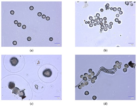
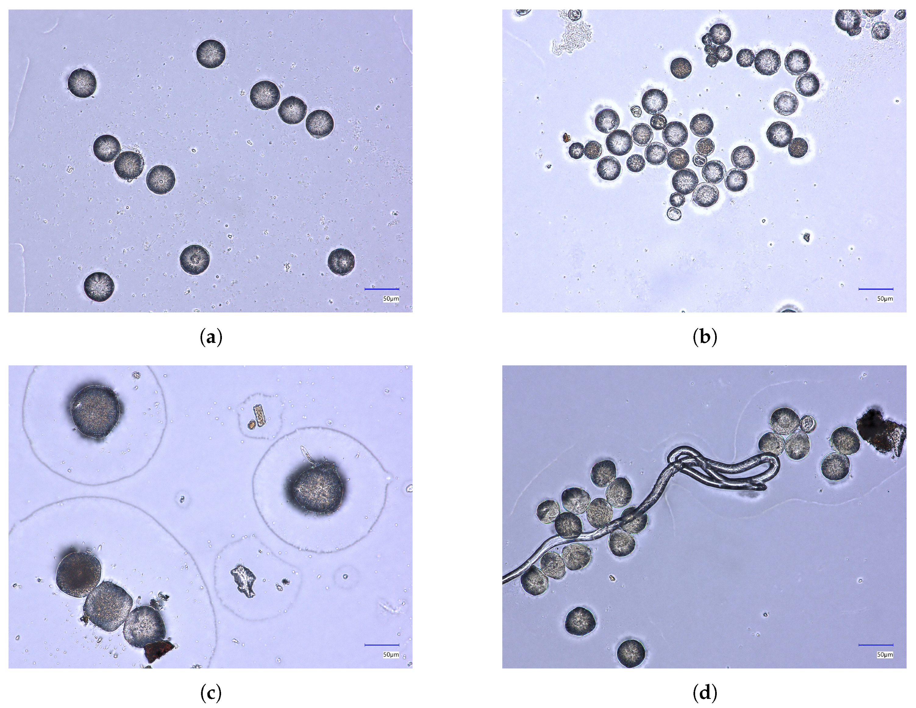
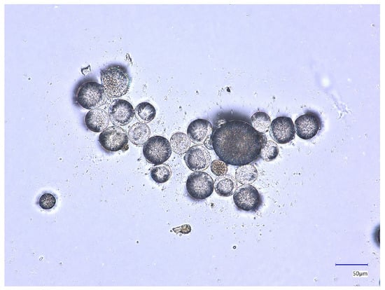
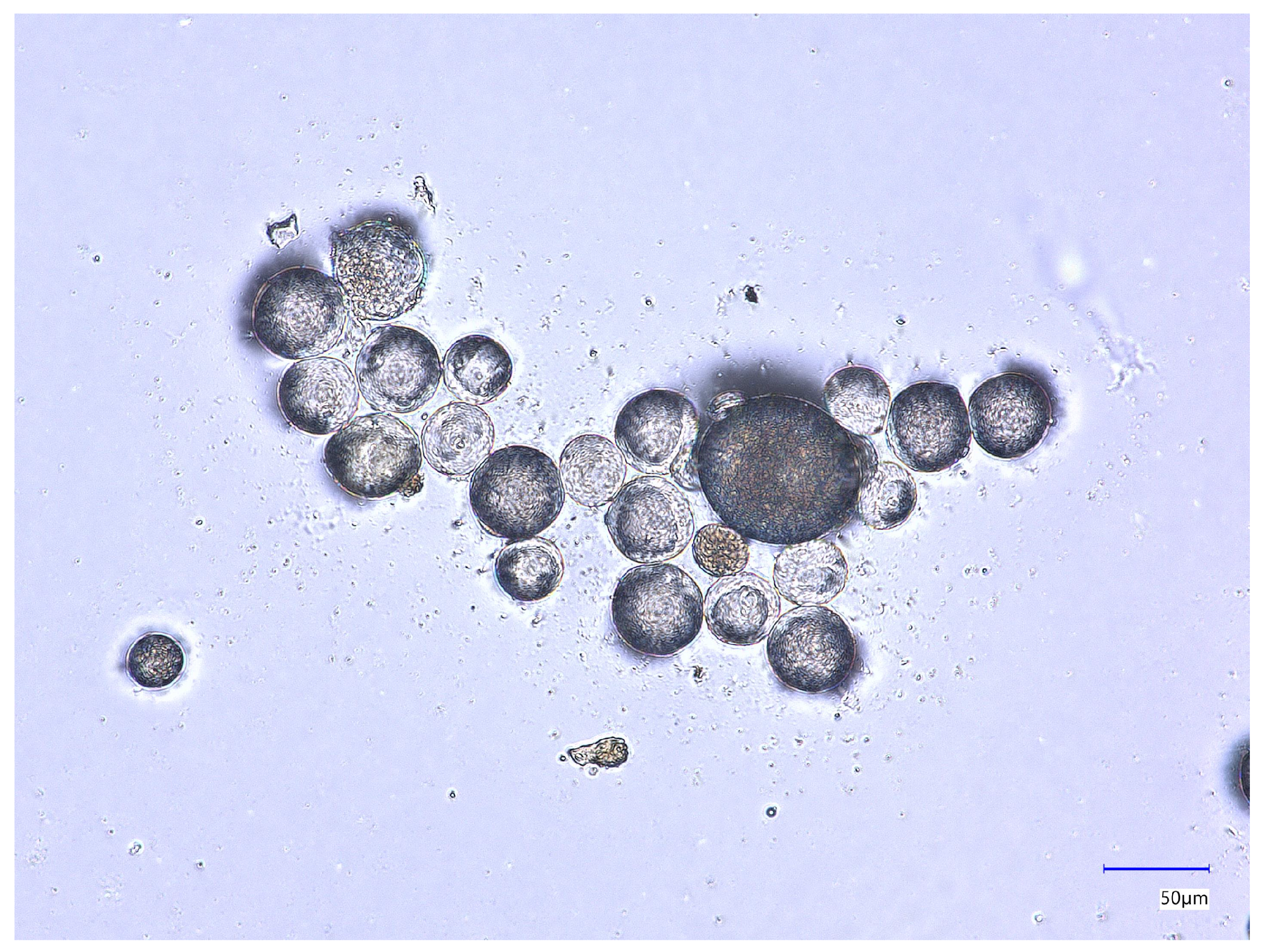
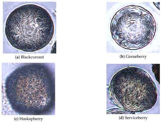
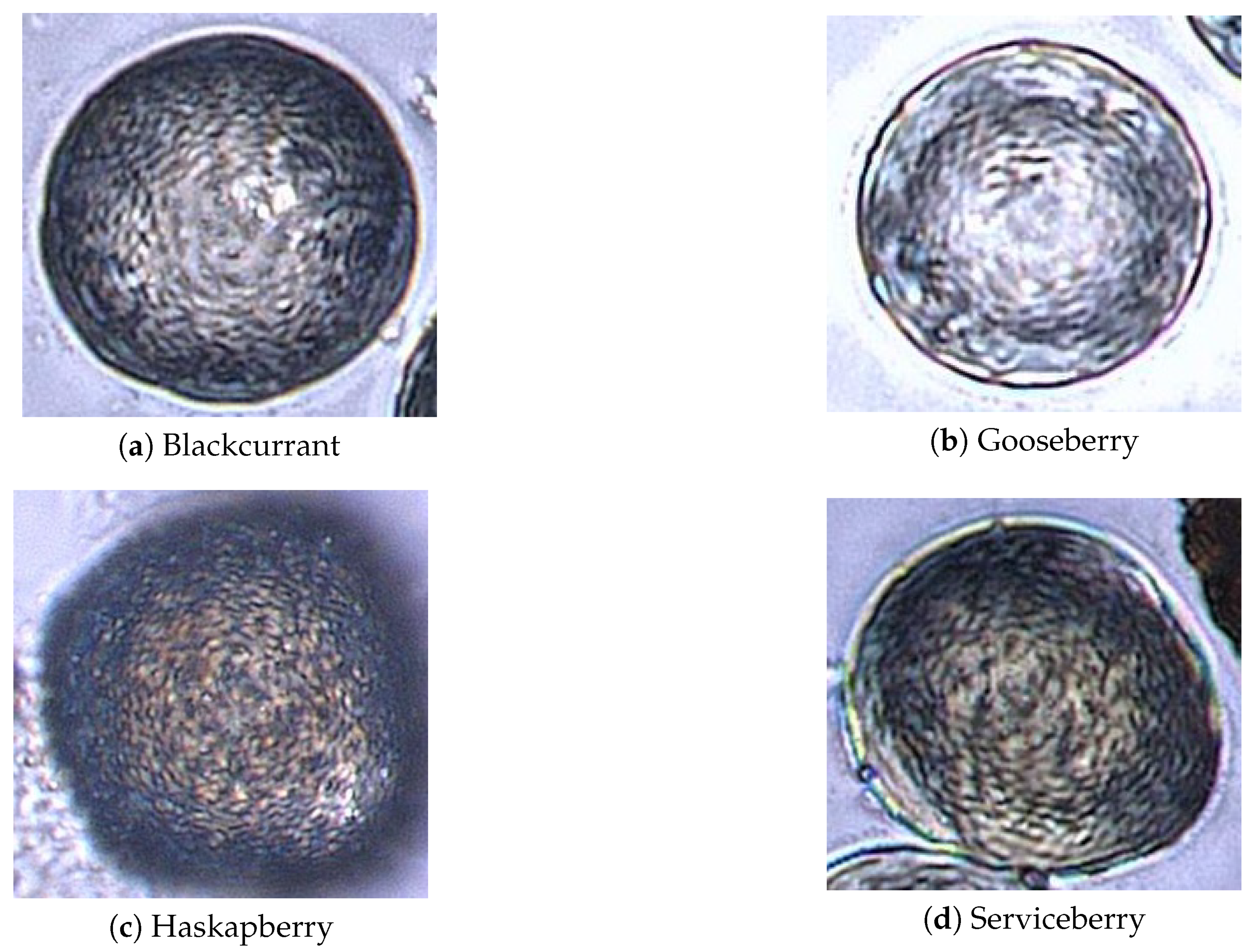
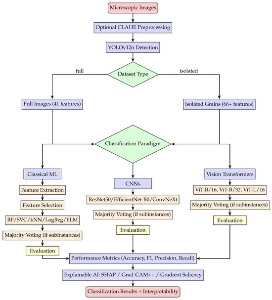
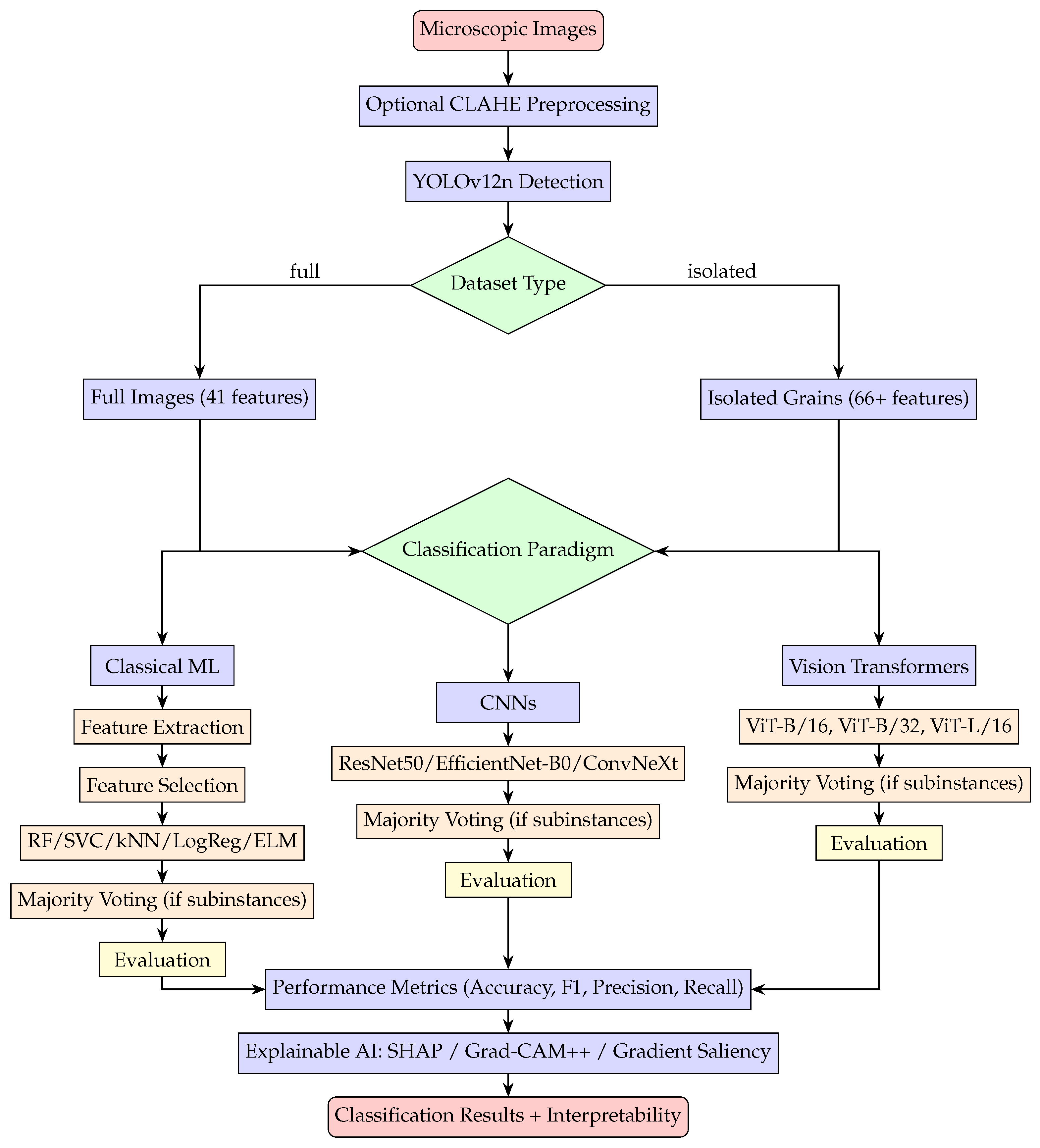
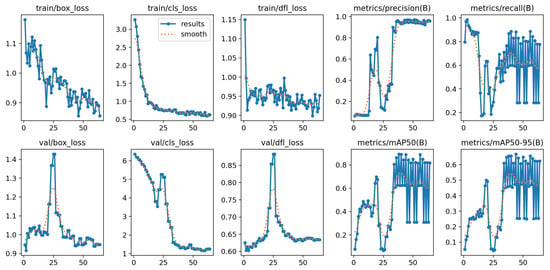
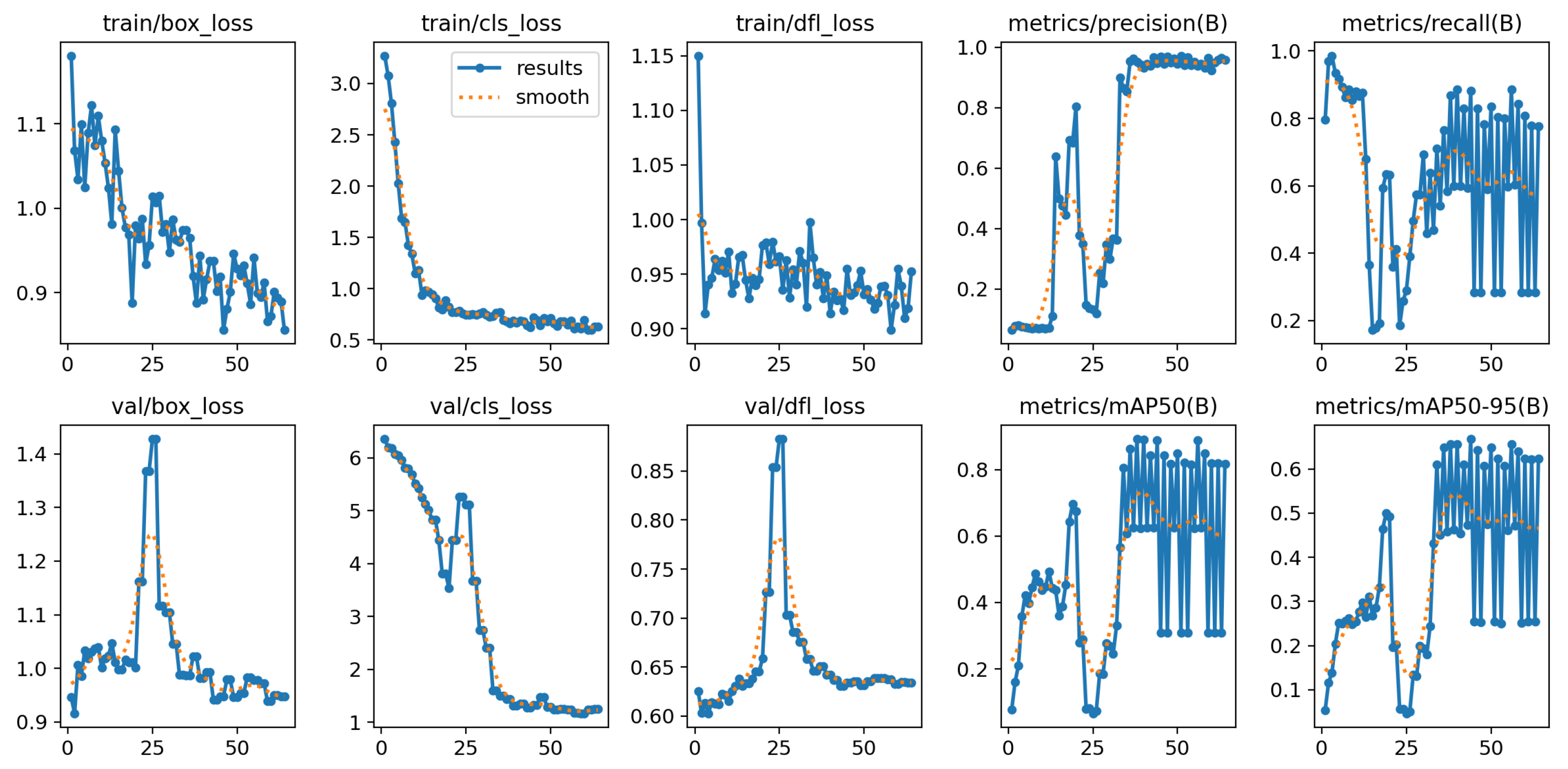
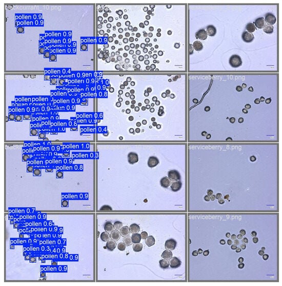
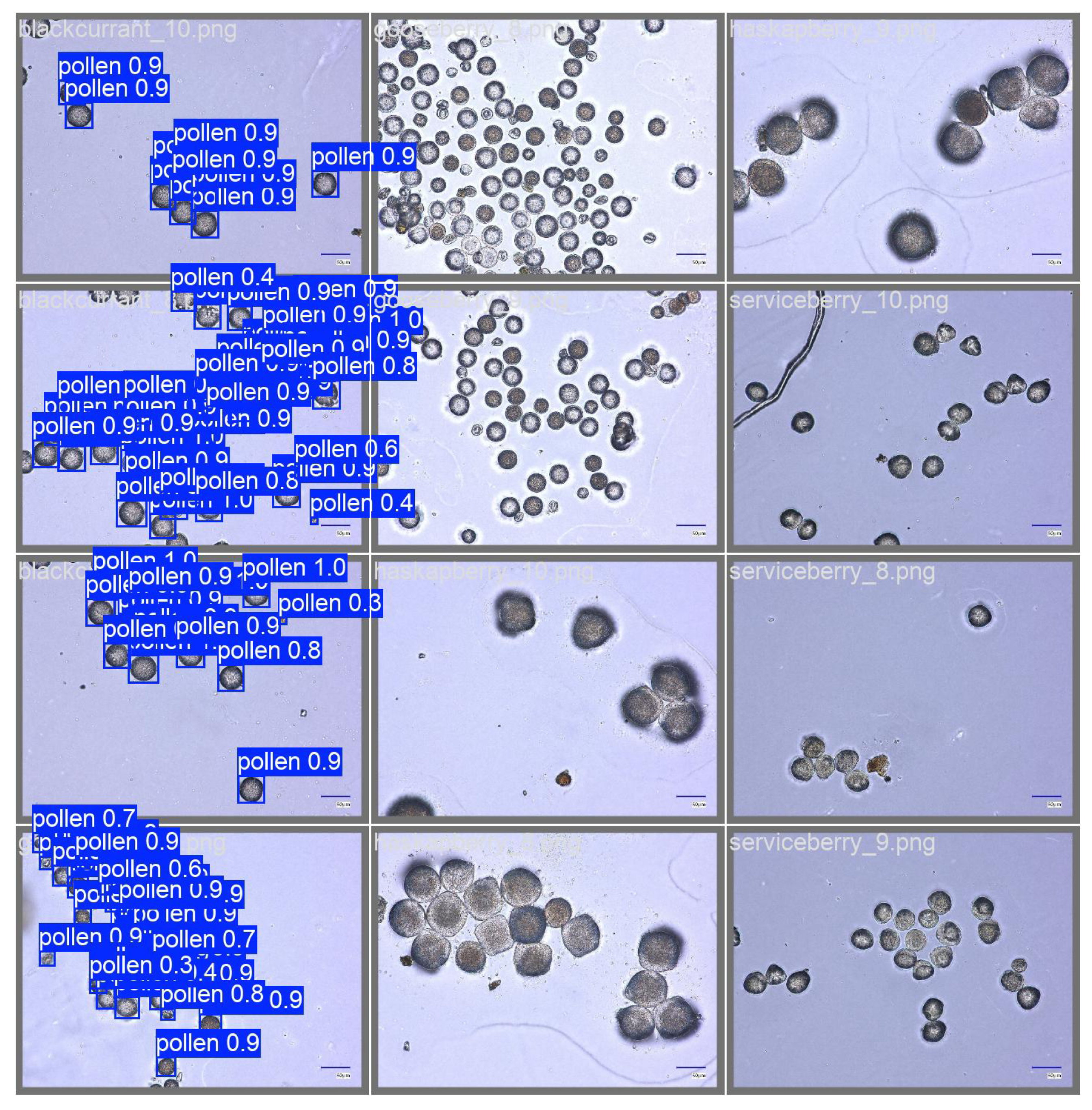
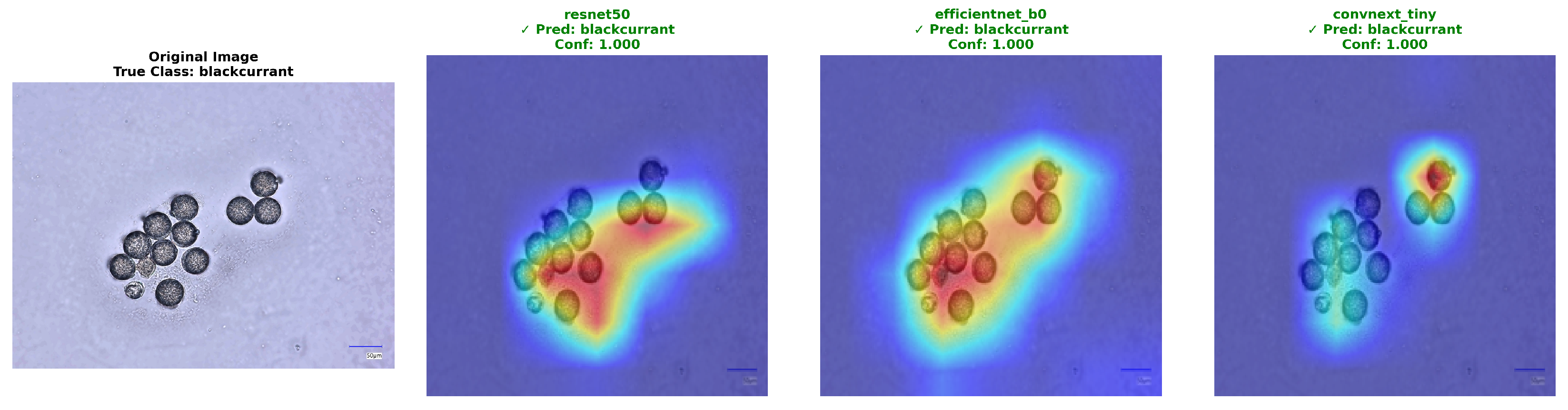
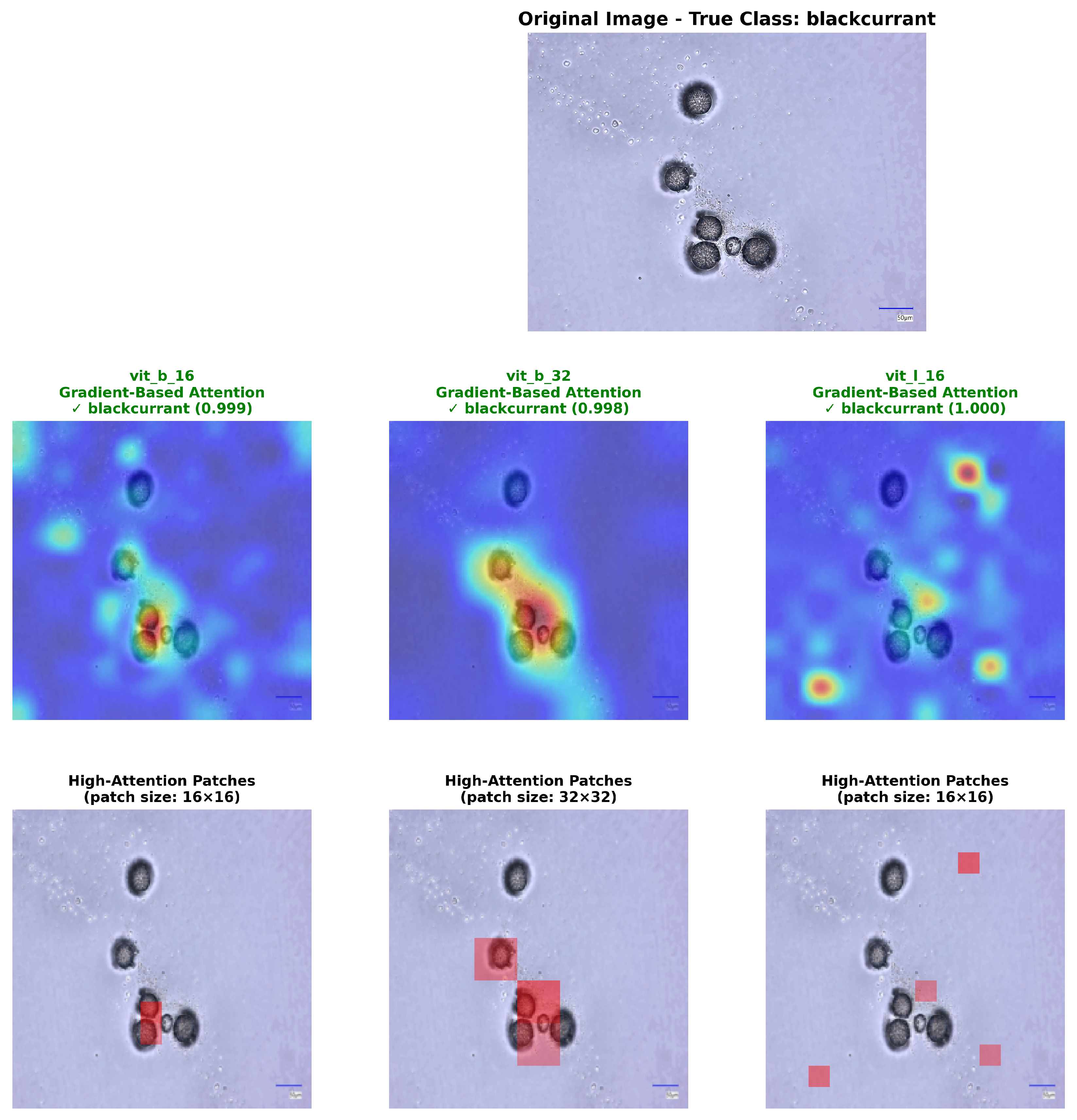

Disclaimer/Publisher’s Note: The statements, opinions and data contained in all publications are solely those of the individual author(s) and contributor(s) and not of MDPI and/or the editor(s). MDPI and/or the editor(s) disclaim responsibility for any injury to people or property resulting from any ideas, methods, instructions or products referred to in the content. |
© 2026 by the authors. Licensee MDPI, Basel, Switzerland. This article is an open access article distributed under the terms and conditions of the Creative Commons Attribution (CC BY) license.