Article

Improved Variational Mode Decomposition for Magnetotelluric Data Denoising Combined with Transformer Neural Network

1
Key Laboratory of Intraplate Volcanoes and Earthquakes (China University of Geosciences, Beijing), Ministry of Education, Beijing 100083, China
2
State Key Laboratory of Deep Earth Exploration and Imaging, School of Geophysics and Information Technology, China University of Geosciences (Beijing), Beijing 100083, China
3
Shanghai Key Laboratory of Submarine Resources, Tongji University, Shanghai 200092, China
4
School of Ocean and Earth Science, Tongji University, Shanghai 200092, China
*
Author to whom correspondence should be addressed.
Appl. Sci. 2026, 16(18), 8931; https://doi.org/10.3390/app16188931
Submission received: 3 August 2026 / Revised: 7 September 2026 / Accepted: 7 September 2026 / Published: 8 September 2026
(This article belongs to the Special Issue Applied Geophysical Imaging and Data Processing, 2nd Edition)

Abstract

Magnetotelluric (MT) transfer-function estimation is severely challenged by strong industrial interference and random noise in complex observation environments. Here, we introduce a hybrid denoising framework that integrates Transformer-based interference identification with particle swarm optimization–variational mode decomposition (PSO-VMD). The Transformer identifies and suppresses strong high-frequency interference while preserving and reconstructing low-frequency signals. PSO-VMD adaptively optimizes the decomposition parameters to isolate and remove noise-dominated components and recover high-frequency signals. By integrating the complementary outputs of the two stages, the proposed framework achieves broadband reconstruction of MT time series. Experiments using synthetic and field data demonstrate that the method robustly suppresses complex interference and noise and substantially improves the accuracy and stability of MT transfer-function estimation. These results demonstrate that the proposed framework provides an effective approach for MT data processing in complex noise environments.

1. Introduction

Magnetotelluric (MT) is a natural-source electromagnetic (EM) geophysical method widely used to investigate subsurface electrical resistivity. Typically, time series of orthogonal EM fields are observed and frequency-dependent transfer functions, including impedance tensors and induction arrows, are estimated using linear regression algorithms [1]. The quality of the estimated transfer functions is essential for obtaining a reliable subsurface resistivity model. Various approaches in the time and frequency domains have been developed over the last few decades [2,3,4,5,6,7,8,9,10,11], some of which are briefly reviewed below.
In general, a typical MT data processing workflow includes the following steps: (1) time series are subdivided into overlapping data segments, followed by cascaded decimation; (2) each data segment is pre-whitened and tapered with a Hanning or Hamming window; (3) Fourier transforms are applied to obtain the Fourier coefficients, which are then corrected for the instrument response; (4) the spectral density matrix is calculated, and data segments are then pre-selected according to coherence and other quality criteria; and (5) regression procedures, generally regarded as robust estimation techniques, are then performed to obtain optimal transfer functions. Based on these basic processing steps, various statistical methods and time-series denoising algorithms have been proposed. In practice, robust estimation techniques, generally implemented in the frequency domain and are based on either the dependent variable (electric field data) [2,4,7,12] or the predictor variable (magnetic field data) [13]. These techniques are often combined with remote-reference methods [2,5,6,14,15]. When synchronously observed array data are available, multivariate linear regression methods, including multivariate robust remote reference estimation techniques [16], frequency-domain independent component analysis [17,18] and principal component analysis [3,19,20], can effectively improve processing quality.
In addition, time-domain approaches have also been developed for MT response estimation and noise suppression. Spagnolini [21] proposed an adaptive time-domain impedance tensor estimation method that improves the robustness of impedance estimates against transient noise. Approaches involving time-series preselection and/or denoising can improve data quality. Santarato and Spagnolini [22] developed a directional noise cancelation technique to identify and suppress impulsive EM interference based on its polarization characteristics. Wavelet transform (WT) and/or Hilbert–Huang transform (HHT) have been employed for data segment preselection [23,24]. More recently, EWT has been applied to non-stationary signal denoising because of its adaptive decomposition capability, demonstrating effective noise suppression while preserving signal characteristics [25]. Polarization analysis in the discrete wavelet domain has also been proposed to identify and suppress temporally localized cultural noise by exploiting differences in the polarization characteristics of natural MT signals and anthropogenic interference [26]. Methods using Wiener filtering with reference data [27] and compressive sensing [28] have been used to replace or reconstruct noisy data segments. However, these approaches may still be ineffective when noise-contaminated data segments dominate.
Furthermore, mode decomposition techniques have been widely used for MT data denoising because of their solid mathematical foundations and strong signal-processing capabilities. Chen et al. [29] applied empirical mode decomposition (EMD), and Li et al. [30] further employed variational mode decomposition (VMD) to improve the robustness of MT data processing. More recently, Guo et al. employed VMD to derive the instantaneous spectrum of non-stationary MT signals and combined it with signal–noise separation techniques to improve the reliability of impedance estimates, particularly for short-duration observations [31]. Unlike EMD, VMD formulates signal decomposition as a constrained variational optimization problem and simultaneously estimates the center frequencies and bandwidths of all modes, resulting in improved decomposition stability and reduced mode mixing [32]. Since the denoising performance of VMD strongly depends on the choice of the mode number and penalty factor, adaptive optimization methods, such as particle swarm optimization (PSO), sparrow search algorithm (SSA), and beluga whale optimization (BWO), have been introduced to optimize these parameters [33,34,35]. Wang et al. [36] combined VMD with wavelet thresholding and mathematical morphology filtering (MMF) to further suppress residual high-frequency noise while preserving useful low-frequency components discarded during decomposition. Nevertheless, VMD-based methods still rely heavily on parameter optimization, and separating strong interference from weak low-frequency MT signals remains challenging under complex noise conditions.
In addition, artificial neural networks have demonstrated advantages in time-series analysis and processing, including noise identification and removal and signal reconstruction and prediction, demonstrating their considerable potential in geoscience [37]. Generally, supervised learning requires manually labeled training data based on predefined criteria (e.g., data quality and signal correlation) [11]. Common neural network architectures, such as convolutional neural networks (CNNs), long short-term memory (LSTM), U-Net, and gated recurrent units (GRUs), have been used either independently or in combination to handle noise and contaminated MT data and suppress EM noise with typical morphological features [9,10,38]. CNNs and U-Net are effective in extracting local and multiscale features, but their ability to model long-range temporal dependencies is relatively limited. LSTM and GRU networks are more suitable for modeling temporal dependencies, although their recurrent structures may increase computational costs and reduce efficiency for long sequences. For instance, Li et al. [10] proposed a two-step method using CNNs for signal–noise separation and an LSTM network for model training using CNN-denoised data. Using an LSTM network, Tian et al. [39] utilized synchronously observed data from a reference station deployed in an underground laboratory as the training set for a data-driven model to reconstruct noisy segments at local stations. Multiple channels can be used in combination for neural network training and noise suppression [40]. More recently, Transformer-based models [41] have demonstrated considerable potential in geophysical and vibration signal processing owing to their ability to capture long-range dependencies and global temporal correlations.
Furthermore, sparse coding and dictionary learning algorithms have been employed for EM noise suppression. Feng et al. [42] developed a K-SVD dictionary learning algorithm to enhance the processing of marine MT signals. A combination of deep convolutional learning classification and dictionary learning denoising has demonstrated advantages in achieving fully adaptive sparse decomposition of MT data [43]. Similar methods integrating mathematical morphology filtering, convolutional networks, sparse coding, and dictionary learning have been developed in previous studies [44,45,46,47]. Generally, repeated trials are often required to determine appropriate parameter values to achieve satisfactory results with these methods, making them challenging to apply in practice.
A common limitation of the aforementioned methods, however, is that misclassification may occur when persistent noise is present in time series or when noise-contaminated and clean data exhibit similar morphological features, making it difficult to distinguish noise from useful signals, particularly at longer periods. Furthermore, the effectiveness and reliability of noise suppression depend heavily on the representativeness of the training data. Inadequate coverage of diverse signal and noise characteristics may compromise the model’s generalization ability when applied to unseen noise patterns.
In this study, we develop a joint MT denoising framework that couples Transformer-based interference identification with PSO-optimized VMD to address strong localized interference and random noise. The Transformer identifies and localizes interference-contaminated segments, which are subsequently removed and reconstructed by linear interpolation. Meanwhile, PSO-VMD adaptively optimizes the number of modes (i.e., the number of intrinsic mode functions) and penalty factor (i.e., a balancing parameter that controls the bandwidth of each mode) for signal decomposition, enabling the separation and removal of noise-dominated components and the recovery of high-frequency MT signals. The outputs of the two complementary denoising pathways are then integrated to reconstruct the final broadband MT time series. By combining the temporal discrimination capability of the Transformer with the adaptive decomposition capability of PSO-VMD, the proposed framework simultaneously suppresses strong interference and random noise while preserving diagnostically important low-frequency information. The resulting improvement in signal quality enhances the robustness of MT transfer-function estimation under complex noise conditions.

2. Theory and Method

2.1. Variational Mode Decomposition

VMD is an adaptive decomposition method for non-stationary signals [32]. It decomposes an input signal f ( t ) (i.e., electric and magnetic components of MT time series) into K band-limited intrinsic mode functions (IMFs), u k ( t ) , characterized by distinct center frequencies ω k . Accordingly, the original signal can be reconstructed as follows:
f t = k = 1 K u k t .
Dragomiretskiy and Zosso [32] provided a detailed mathematical formulation and solution procedure for VMD. Here, we briefly review the basic procedure. The analytic signal of each mode is first obtained using the Hilbert transform [48] and then demodulated to the baseband using its center frequency, allowing its bandwidth to be estimated. VMD subsequently minimizes the sum of the estimated bandwidths subject to the reconstruction constraint in Equation (1). By introducing a quadratic penalty factor α and a Lagrange multiplier function, the constrained problem is reformulated as an augmented Lagrangian problem and solved using the alternating direction method of multipliers (ADMM) [32,49,50]. The modal components and their center frequencies are iteratively updated until the convergence criterion is satisfied.
The decomposition performance of VMD is affected by the mode number K and the penalty factor α . Improper selection of these parameters may lead to under-decomposition, over-decomposition, or poor mode separation [51]. Therefore, PSO is introduced to adaptively optimize K and α .

2.2. PSO-Based Optimization of VMD Parameters

2.2.1. Basic Principle of PSO

PSO is a population-based intelligent optimization algorithm inspired by the foraging behavior of bird flocks [52]. In PSO, each candidate solution is regarded as a particle in the search space. Each particle has two attributes: positions and velocities. During iteration, particles update their search directions according to their individual best positions and the global best position of the swarm [52].
Assume that the positions and velocities of the i -th particle at the t -th iteration are x i t and v i t , respectively. The individual best position is denoted by p i , and the global best position is denoted by g . The velocity and position are updated as follows:
v i t + 1 = v i t + c 1 r 1 p i x i t + c 2 r 2 g x i t ,
x i t + 1 = x i t + β v i t + 1 ,
where c 1 and c 2 are learning factors, r 1 and r 2 are random numbers uniformly distributed in [0, 1], and β is a step-size factor. Through iterative updates, the particle swarm gradually approaches the optimal solution.

2.2.2. PSO-VMD Parameter Optimization

In the proposed PSO-VMD method, each particle represents a candidate parameter combination:
x i = K i , α i ,
where K i is the candidate mode number and α i is the candidate penalty factor. For each particle, VMD is performed using the corresponding parameter combination, and the decomposition quality is evaluated using a fitness function.
First, the reconstructed signal is obtained by summing all the IMFs, and the reconstruction error is calculated as follows:
E r e c = 1 L t = 1 L f t k = 1 K u k t 2 ,
where L is the signal length, f ( t ) is the input signal, and u k ( t ) is the k -th IMF obtained by VMD.
To evaluate the concentration of the noise component in a specific IMF, the noise concentration index is defined as follows:
C = ρ k n R n 1 ρ ¯ o ,
where ρ k = c o r r u k ( t ) , n ( t ) , t Ω n , is the absolute correlation coefficient between the k -th IMF and the detected noise pattern n ( t ) within the detected noise region Ω n . The dominant noise mode is determined as k n = a r g m a x k ρ k , and ρ k n is the corresponding maximum correlation coefficient. The term
R n = t Ω n u k n 2 t k = 1 K t Ω n u k 2 t ,
denotes the proportion of energy associated with the dominant noise mode within the detected noise region, and ρ ¯ o is defined as follows:
ρ ¯ o = 1 K 1 k = 1 k k n K ρ k .
The three factors in Equation (6) characterize complementary aspects of noise concentration. Specifically, ρ k n measures the similarity between the dominant noise mode and the detected noise pattern, while R n characterizes the energy concentration of the dominant noise mode within Ω n . In contrast, ρ ¯ o reflects noise-related components in the remaining modes, and 1 ρ ¯ o therefore quantifies noise leakage. The multiplicative form ensures that a high C is obtained only when the noise is strongly correlated and energetically concentrated in the dominant mode, with limited leakage into the remaining modes. Since all three factors are bounded between 0 and 1, C satisfies: 0 C 1 .
The theoretical maximum C = 1 corresponds to the ideal case where ρ k n = 1 , R n = 1 , and ρ ¯ o = 0 . In this scenario, the dominant noise mode is perfectly correlated with the detected noise pattern, the modal energy within the detected noise region is concentrated in this mode, and the remaining modes contain no correlated noise component. For practical signals, C is generally smaller than 1, and a larger C indicates a higher concentration of the detected noise component in a single mode with less leakage into the remaining modes.
The modal energy entropy is calculated as follows:
H = k = 1 K p k ln p k ,
p k = E k j = 1 K E j ,
E k = t = 1 L u k 2 t ,
where p k denotes the normalized energy fraction of the k -th IMF. Lower energy entropy indicates a more concentrated modal energy distribution.
Accordingly, the fitness function is formulated as follows:
F = w 1 E r e c + w 2 1 C + w 3 H .
The weighting coefficients are set to w 1 = 0.3 , w 2 = 0.5 , and w 3 = 0.2 , with w 1 + w 2 + w 3 = 1 . Following the weighted-sum principle [53], the weights reflect the relative importance of the three criteria. A larger weight is assigned to the noise concentration term, as concentrating the noise component in a specific mode is the primary objective of the proposed method, while reconstruction fidelity and modal energy distribution are treated as complementary criteria. Finally, the optimal VMD parameters are obtained by minimizing the fitness function:
K * , α * = a r g min K , α F ,
In this study, the particle population size and maximum number of iterations are set to 18 and 10, respectively. The PSO search ranges for the optimal VMD parameters are K 2 ,   12 and α 1000 ,   8000 . These ranges were selected to cover practical and meaningful decomposition conditions while avoiding excessive under-decomposition or over-decomposition [54]. For VMD, τ = 0 , D C = 0 , i n i t = 1 , and t o l = 10 7 are adopted, following the conventional VMD implementation [32]. These settings are consistent with the uploaded implementation. The detailed procedure is summarized in Algorithm 1.
Algorithm 1: PSO of VMD Parameters
Input: MT time series f(t), search ranges of K and α, population size N, maximum number of iterations G, learning factors c 1 and c 2 , and step-size factor β.
Output: Optimal VMD parameters K * ,   α * .
1. Initialize particle positions x i 0 = [ K i 0 , α i 0 ] and velocities v i 0 , i = 1,2 , , N ;
2. For each particle, perform VMD using x i 0 = [ K i 0 , α i 0 ] ;
3. Calculate the fitness value:
                                                    F i = w 1 E r e c + w 2 1 C + w 3 H ;
4. Set the personal best position p i = x i 0 , and set the global best position as the position of the particle with the minimum fitness value;
5. while g   < G and the stopping criterion is not satisfied do
6.         g = g + 1
7.         for i = 1 : N do
8.                Update particle velocities:
                                     v i g = v i g 1 + c 1 r 1 p i x i g 1 + c 2 r 2 x b e s t x i g 1 ;
9.                Apply velocity constraints;
10.              Update particle position:
                                                                x i g = x i g 1 + β v i g ;
11.                Apply boundary constraints to K i g and α i g ;
12.                Perform VMD decomposition using the updated x i g = [ K i g , α i g ] ;
13.                Calculate the current fitness value F i g ;
14.       end for
15.       for i = 1 : N do
16.             if F i g < F ( p i )   then
17.                 p i = x i g
18.             end if
19.             if F i g < F x b e s t   then
20.                 x b e s t = x i g
21.             end if
22.         end for
23. end while
24. Return x b e s t = [ K * , α * ] .
Finally, the optimal particle g is selected as the optimal VMD parameter combination K * α * . Compared with empirical parameter selection, the PSO-based strategy can automatically search for suitable VMD parameters, thereby improving the adaptivity and stability of VMD for non-stationary MT signals.

2.3. Intelligent Filtering

To further suppress transient spike interference while preserving the underlying MT signal, an intelligent filtering strategy is applied to the reconstructed signal obtained from VMD. Instead of directly removing abnormal samples, the proposed method first detects transient spike regions using multiple complementary criteria and then reconstructs these regions according to the local statistical characteristics of neighboring normal samples. Specifically, the reconstructed signal is first obtained as follows:
y t = k = 2 K u k t ,
where u k ( t ) denotes the k -th IMF. The first IMF, which mainly contains low-frequency noise, is excluded from the reconstruction. To identify abnormal samples, amplitude, local statistical deviation, and signal gradient are jointly considered. The local trend is first estimated using a median filter [55]:
m t = M e d F i l t y t } ,
where MedFilt{·} denotes the median filtering operator with a specified window length, and m(t) represents the estimated local trend of the reconstructed signal. Three detection masks are then constructed based on amplitude, local deviation, and gradient, respectively. The final spike mask is obtained as follows:
M t = M a t M s t M g t ,
where M a ( t ) , M s ( t ) , and M g ( t ) denote the amplitude-, statistical-, and gradient-based detection masks, respectively. The detected regions are subsequently expanded using morphological dilation to ensure complete coverage of the transient interference.
For each detected abnormal region, the local trend is estimated using a median filter, while the local fluctuation is synthesized using a first-order autoregressive (AR(1)) process estimated from the surrounding normal signal [56]:
z t = ϕ z t 1 + ε t ,
where ϕ is the autoregressive coefficient and ε ( t ) is a Gaussian innovation term. The reconstructed signal within the abnormal region is then generated as follows:
y ^ t = m t + z t ,
where m ( t ) denotes the local trend estimated from neighboring normal samples. Finally, to avoid abrupt discontinuities between the reconstructed and original signal segments, a weighted transition is applied over a short interval on both sides of each reconstructed region. Within the transition interval, the reconstructed signal is gradually blended with the original signal using smoothly varying weights. A Savitzky–Golay filter [57,58] is then applied to further suppress local fluctuations introduced by the reconstruction and to improve signal continuity. The reconstructed signal can be expressed as follows:
y f t = y ^ ( t ) , t Ω n y t , t Ω n ,
where Ω n denotes the detected abnormal region.
In this study, the filtering parameters were selected according to the temporal scale and statistical characteristics of the transient spike interference. The gradient threshold was adaptively determined as the 99.5th percentile of the gradient distribution to identify unusually abrupt variations. The detected intervals were subsequently expanded to cover the transition regions of the spikes, while neighboring normal samples were used for AR(1) estimation. Finally, Savitzky–Golay smoothing was applied locally to reduce discontinuities introduced by signal reconstruction.

2.4. Transformer-Based Noise Identification

An Anomaly Transformer model [59] is used to identify strong interference in MT time series. Given an input sequence X R N × d , token embedding and positional embedding are first applied to obtain high-dimensional temporal features. The embedded sequence is then fed into stacked Transformer encoder layers, which consist of anomaly-attention modules, feed-forward networks, residual connections, and layer normalization. The structure of the Anomaly Transformer used for time-series noise identification is shown in Figure 1.
To enable the Transformer model to learn the intrinsic temporal characteristics of MT signals, a dedicated noise identification dataset was constructed before model training. The original MT observations were first normalized using Z-score normalization to reduce amplitude differences among channels. Subsequently, a sliding-window strategy was adopted to segment the continuous time series into fixed-length samples, each containing local temporal information and long-range correlation characteristics.
The constructed dataset mainly consists of MT signals with weak interference, which are regarded as normal patterns for unsupervised anomaly detection. The model learns the temporal association characteristics of normal MT signals during training without requiring manual labels. During testing, typical strong interference signals, including abrupt disturbances and pulse-like noise, are selected and labeled to evaluate the ability of the trained model to identify abnormal segments.
After training, the Transformer model generates anomaly scores based on the discrepancy between the prior association and series association. Segments with high anomaly scores are identified as strong-interference segments and are subsequently processed in the denoising procedure.
The core component of the model is the anomaly-attention mechanism, which simultaneously models global temporal dependencies and local neighborhood dependencies. Specifically, the hidden features from the previous layer are linearly projected to generate the query, key, value, and learnable scale parameter: Q = X W Q , K = X W K , V = X W V , and σ = X W σ . Based on the learnable scale parameter, a Gaussian kernel is employed to construct the prior association, which explicitly characterizes the local correlation around each timestamp:
P i , j l = 1 2 π σ i exp j i 2 2 σ i 2 .
Meanwhile, the series association is obtained using the standard self-attention mechanism [41], in which the scaled query-key similarities are normalized by the softmax function to obtain the attention weights:
S = S o f t m a x Q K T d m o d e l ,
where the softmax function is defined as S o f t m a x z i = e x p z i / j = 1 n e x p z j for a vector z = z 1 ,   ,   z n .
For normal MT signals, long-range temporal dependencies dominate the sequence, resulting in a noticeable discrepancy between the prior association and the series association. In contrast, strong interference noise is generally characterized by impulsive and locally continuous patterns, causing the learned series association to concentrate on local neighborhoods and become more similar to the prior association. Therefore, the discrepancy between the two associations can effectively distinguish abnormal interference from normal MT signals. Following the original Anomaly Transformer, the association discrepancy is quantified using the symmetric Kullback–Leibler (KL) divergence [60],
AssDis P , S = 1 L l = 1 L KL P l S l + KL S l P l ,
where P and S denote the prior association and series association, respectively; P l and S l represent the corresponding association distributions at the l -th Transformer encoder layer; L is the total number of Transformer encoder layers; and K L denotes the Kullback–Leibler divergence. Accordingly, A s s D i s P S represents the layer-averaged association discrepancy between the prior and series associations.
To improve the robustness of noise identification, the association discrepancy is further combined with the sequence reconstruction error to calculate the anomaly score:
S c o r e X = S o f t m a x A s s D i s | X X ^ | 2 2 ,
where X and X ^ denote the input and reconstructed sequences, respectively; A s s D i s is the association discrepancy defined in Equation (22); S o f t m a x A s s D i s is used as the normalized association-discrepancy-based weighting term; denotes the Hadamard product (element-wise multiplication); and | | 2 2 denotes the squared L 2 -norm used to quantify the sequence reconstruction error. Time points with anomaly scores exceeding a predefined threshold are identified as strong-interference points. The detected noise intervals are subsequently used as prior information in the subsequent denoising stage, enabling the proposed framework to suppress interference while preserving the intrinsic characteristics of MT signals.

2.5. Workflow of the Proposed Method

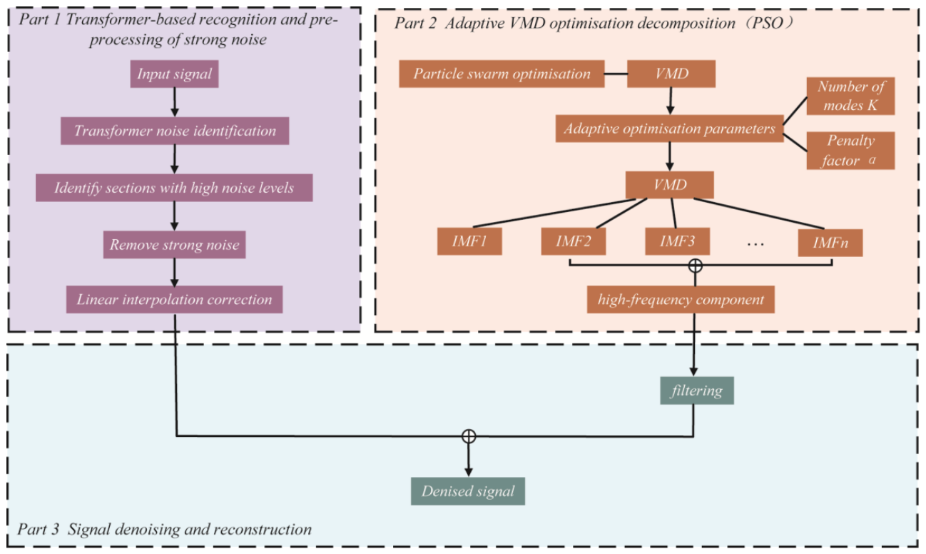
The proposed framework consists of three main stages: Transformer-based strong interference identification and preprocessing, PSO-optimized adaptive VMD and filtering, and final signal reconstruction. The workflow is shown in Figure 2.
First, the original MT time series is fed into the trained Transformer-based anomaly detection model. The model identifies strong interference segments based on anomaly scores, and the detected abnormal segments are removed and reconstructed using linear interpolation to suppress impulsive noise while maintaining signal continuity. Although linear interpolation may introduce uncertainties in the reconstructed segments, the resulting uncertainties are limited because this operation is performed on the long-period trend and the interpolation intervals are generally short.
Second, the original signal is decomposed by VMD, with PSO adaptively optimizing the mode number K and penalty factor α . The optimized VMD results are analyzed according to their spectral characteristics; noise-dominated components are removed, while the remaining components are retained for further filtering.
Finally, the filtered VMD reconstruction components are combined with the linearly interpolated Transformer output to reconstruct the final denoised MT signal. The proposed framework integrates Transformer-based strong interference identification and adaptive PSO-VMD, enabling simultaneous suppression of impulsive interference and random high-frequency noise.

3. Implementation

3.1. Synthetic Experiment

Synthetic time series corresponding to complex geoelectrical structures generally require a relatively complex procedure, including forward modeling, an assumed magnetic source, and an inverse Fourier transform, which is beyond the scope of the present study. Thus, high-quality observed data have been used as noise-free data in previous studies [8,37]. In this study, we used example MT data from the open-source EMTF package [61] to evaluate the proposed method. This dataset has been widely used for validating and evaluating various MT data processing methods [10,43]. Five orthogonal electric and magnetic channels with a sampling rate of 1 Hz and a total duration of 10,000 s were used. Although the time series corresponds to a simple uniform 100 Ω·m half-space model, the synthetically noise-contaminated dataset can still represent typical MT field conditions.
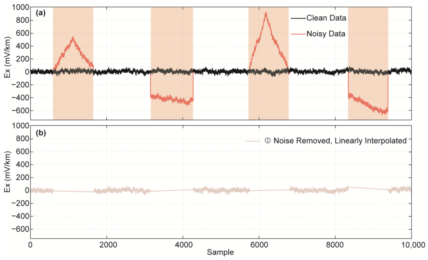
The horizontal electric field component Ex was selected as the test signal. To simulate strong interference conditions commonly encountered in practical MT observations, triangular and tilted-top square noise signals were artificially introduced into the clean Ex time series. The four noise segments were located at approximately (550 to 1664) s, (3150 to 4299) s, (5750 to 6816) s, and (8350 to 9450) s, with amplitudes of approximately (+500, −450, +830, and −530) mV/km, respectively. These artificial disturbances were designed to represent the strong transient interference with different polarities and amplitudes typically observed in field MT data.
Figure 3 presents the Transformer-based identification results for strong interference noise and the subsequent signal reconstruction process. As shown in Figure 3, the Transformer model identifies interference segments with different waveform characteristics, polarities, and amplitudes, demonstrating its capability to capture abnormal temporal patterns and distinguish strong interference from normal MT signal fluctuations. Based on the identified noise locations, the abnormal segments were removed and the missing intervals were subsequently reconstructed using linear interpolation, as shown in Figure 3b. After noise removal, the reconstructed Ex signal eliminates the large-amplitude deviations caused by strong interference while preserving the continuity and overall variation trend of the original MT response. These results indicate that the proposed Transformer-based method can effectively locate strong interference in MT data and provide reliable preprocessing for subsequent signal analysis and denoising.
Before VMD, the key parameters of VMD, including the number of modes K and the penalty factor α , were optimized using the particle swarm optimization (PSO) algorithm. The population size was set to 18, and the maximum number of iterations was set to 10. The search ranges for K and α were defined as [2,12] and [1000, 8000], respectively. The fitness function was constructed based on the decomposition performance of VMD, where a lower fitness value indicates better decomposition performance.
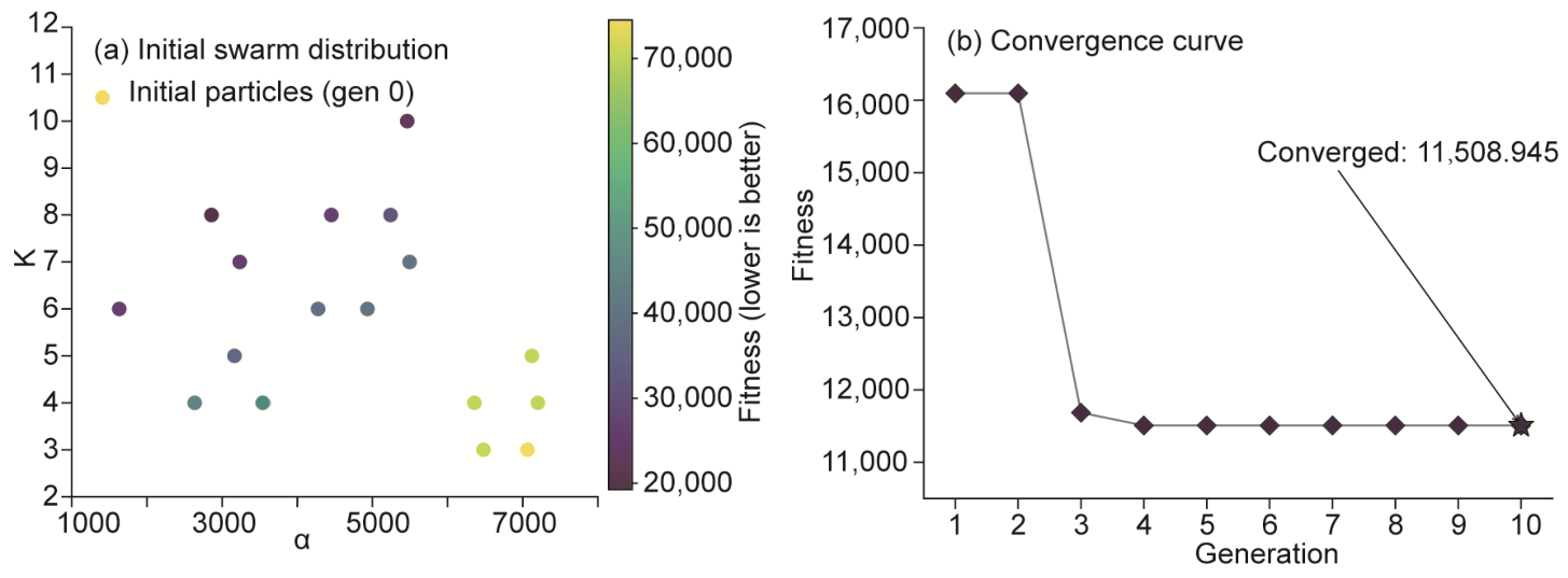
As shown in Figure 4a, 18 particles are randomly initialized within the search space, with each particle corresponding to a parameter combination and its associated fitness value. The particle positions are then iteratively updated based on their individual best positions and the global best position, enabling the swarm to progressively search for parameter combinations with lower fitness values. As shown in Figure 4b, the optimal fitness value decreases rapidly during the early iterations and then gradually stabilizes, eventually converging to 11,508.945, with the corresponding optimal parameters of K = 8 and α = 2000 . These optimized parameters were subsequently adopted for VMD of the noisy Ex signal.
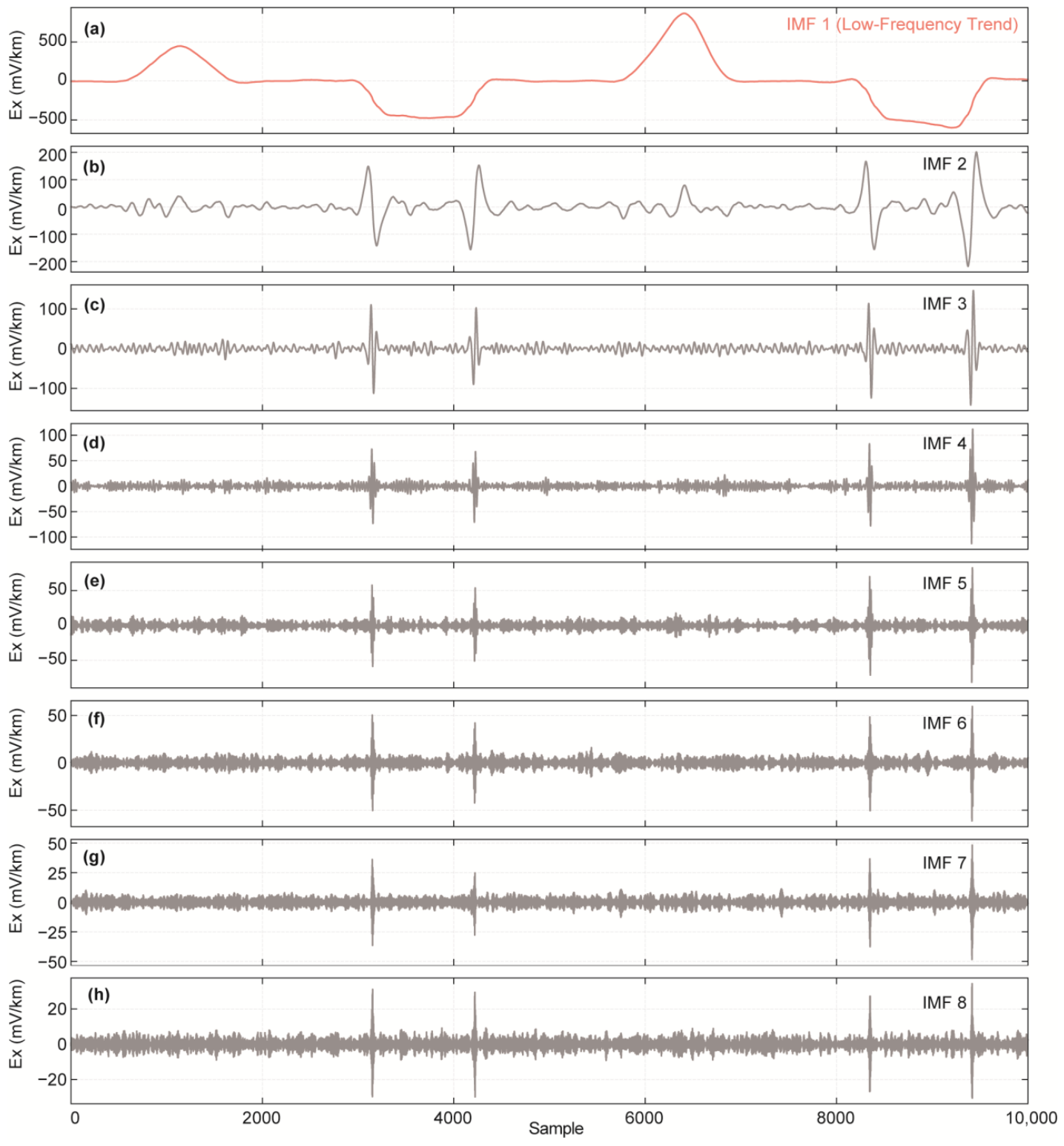
After determining the optimal VMD parameters through PSO, the original noisy MT Ex signal was decomposed using the PSO-VMD method. As shown in Figure 5, the signal was adaptively decomposed into eight intrinsic mode functions (IMFs), each representing different frequency characteristics of the original signal. The first mode (IMF1, Figure 5a) exhibits significant amplitude variations corresponding to the artificially introduced strong interference and was therefore identified as the noise-dominated mode. Thus, IMF1 was excluded, while the remaining IMFs (IMF2–IMF8) were retained for signal reconstruction.
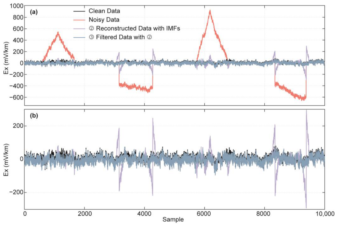
The remaining modal components (IMF2–IMF8) were then reconstructed to preserve useful signal information distributed over different frequency bands (Figure 6). However, the reconstructed signal still contained residual high-frequency fluctuations caused by weak interference and random noise. Therefore, an additional filtering operation was applied to the reconstructed high-frequency signal to suppress these residual noise components before the final signal reconstruction. Figure 6b compares the clean signal, the reconstructed high-frequency signal before filtering, and the filtered high-frequency signal, demonstrating that the filtering operation effectively suppresses residual random noise while preserving the useful high-frequency characteristics required for subsequent signal reconstruction.
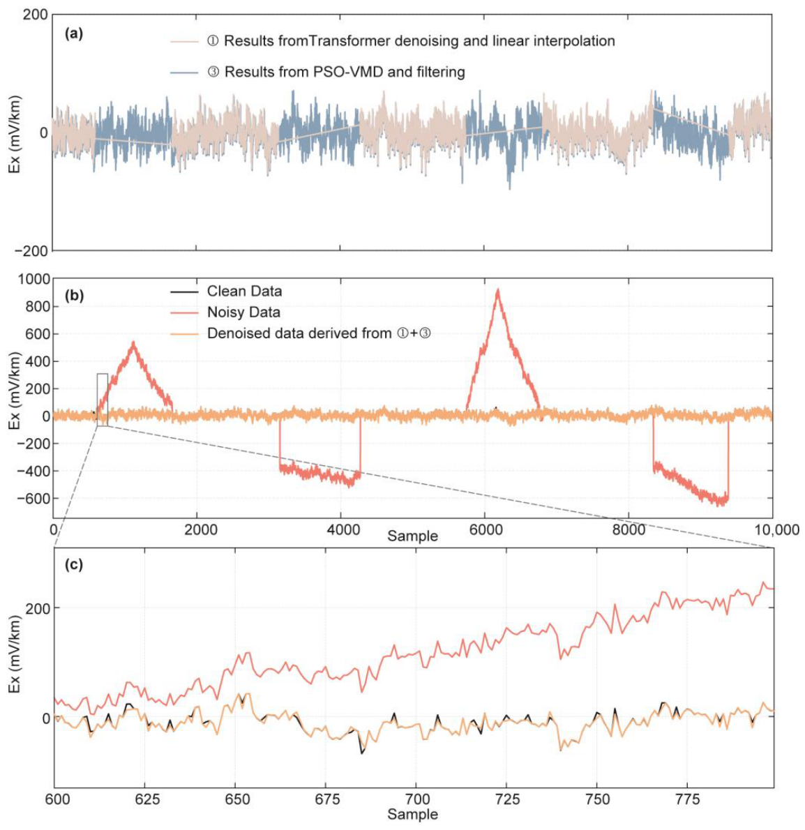
After obtaining the filtered high-frequency components from PSO-VMD, they were selectively superimposed on the signal repaired through Transformer-based interference identification and linear interpolation, as illustrated in Figure 7. Specifically, the filtered high-frequency components were added only within the strong interference intervals identified by the Transformer model, in which the original signal had been removed and reconstructed using linear interpolation. Outside these repaired intervals, the original MT signal was retained without any modification. Consequently, the proposed strategy reconstructs only the contaminated segments while preserving the original waveform characteristics in the uncontaminated regions.
The final denoising results are presented in Figure 7b,c. Compared with the noisy MT signal, the proposed method effectively removes strong interference while further suppressing residual random fluctuations. As shown in the enlarged comparison in Figure 7c, the reconstructed signal agrees well with the clean signal in both waveform and amplitude within the reconstructed interval, indicating that the proposed local reconstruction strategy effectively restores the contaminated segments without introducing noticeable distortions into the surrounding signal.
These results demonstrate that the proposed hybrid denoising framework effectively combines Transformer-based temporal interference localization with PSO-VMD-based adaptive random noise suppression. The Transformer model accurately identifies strong interference intervals, while PSO-VMD extracts and filters useful high-frequency components, which are subsequently used to reconstruct the contaminated intervals. By restricting the reconstruction process to the detected interference regions, the proposed method effectively suppresses noise while preserving the original characteristics of uncontaminated MT signals.
To quantitatively evaluate the denoising performance, the signal-to-noise ratio (SNR), root mean squared error (RMSE), and percent root-mean-square difference (PRD) are employed as evaluation metrics and are calculated as follows:
S N R = 10 l o g 10 n = 1 L f 2 n n = 1 L f n f d n 2 ,
R M S E = 1 L n = 1 L f n f d n 2 ,
P R D = n = 1 L f n f d n 2 n = 1 L f 2 n × 100 % ,
where f n and f d n denote the original and denoised signals, respectively, and L is the signal length. A higher SNR and lower RMSE and PRD values indicate better denoising performance.
We employed the intermediate stages of the proposed framework as independent methods, including Transformer, PSO-VMD, and PSO-VMD-filter, to evaluate the progressive improvement in denoising performance. Additionally, results obtained using the classical EMD [29] and EWT [25] were included for comparisons. As shown in Table 1, the proposed Transformer–PSO-VMD-filter method achieves the highest SNR of −5.6829 dB, the lowest RMSE of 31.92 mV/km, and the lowest PRD of 192.3750%. These results indicate that the proposed method achieves the best overall performance among the compared methods in terms of signal quality, reconstruction error, and relative distortion.
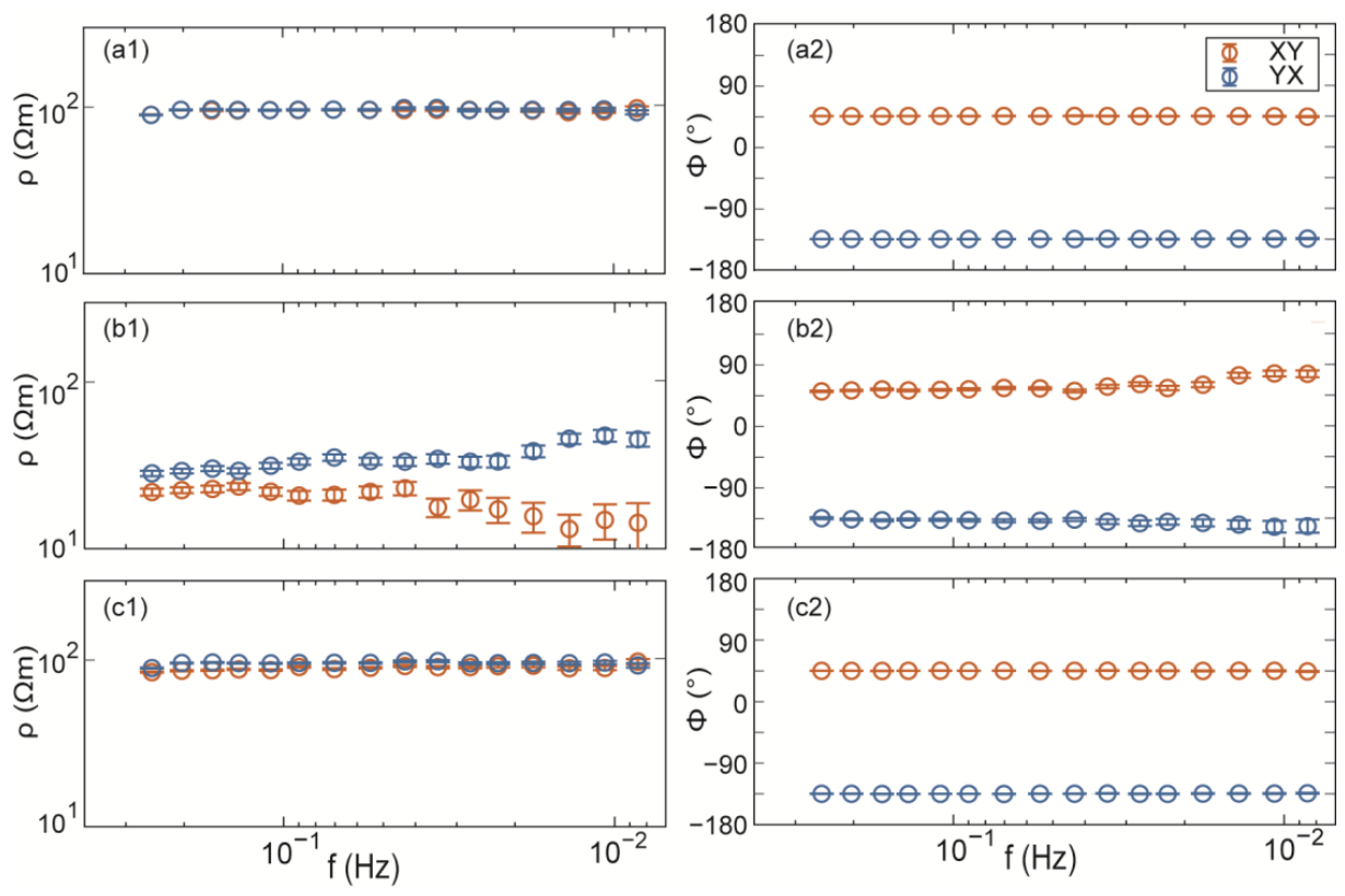
To further evaluate the effectiveness of the proposed denoising method in MT response estimation, the same noise contamination and denoising procedures were applied to all five MT components. The impedance tensors were then estimated using the EMTF package [61] for the clean, noisy, and denoised five-component datasets. Figure 8 shows the apparent resistivity and impedance phase curves obtained from these three datasets. Theoretically, an apparent resistivity of 100 Ω·m and an impedance phases of 45° and/or 145° correspond to a uniform half-space (Figure 8(a1,a2)). For the noisy data, the apparent resistivity and impedance phase curves exhibit obvious distortions: the resistivity responses of both xy and yx modes deviate significantly from the theoretical value of 100 Ωm over the entire frequency range (Figure 8(b1)), and the impedance phases show substantial deviations from the expected 45° and/or 145° response, especially in the longer-period band (Figure 8(b2)). In contrast, the results obtained from the denoised data show good agreement with those from the clean data in both the apparent resistivity and impedance phase (Figure 8(c1,c2)). These results demonstrate that the proposed combined Transformer–PSO-VMD denoising method can effectively suppress strong interference and random noise while preserving the characteristics of the underlying MT response.

3.2. Field Data Experiment

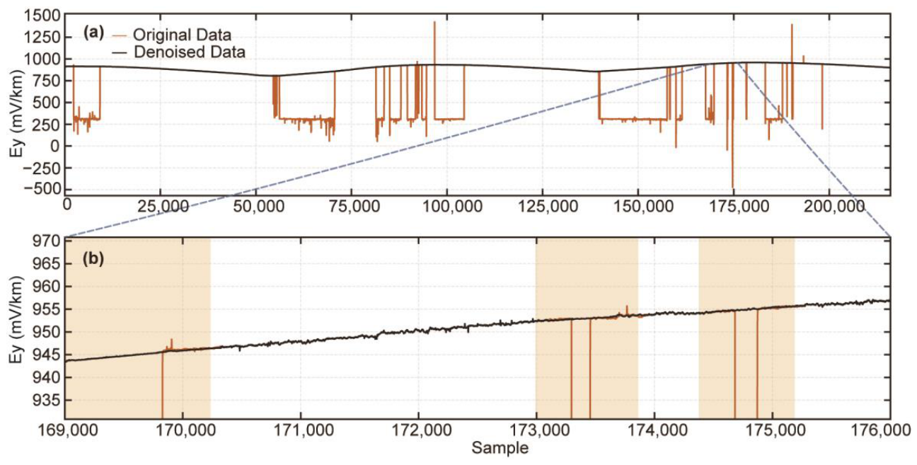
To further verify the applicability of the proposed method under complex real-world observation conditions, field MT time-series data collected in southern Tibet using a LEMI-417 system were used for denoising experiments. Five orthogonal data components, including three magnetic channels and two electric channels, were recorded at a sampling rate of 1 Hz. The east–west-oriented electric field (Ey) was contaminated by random noise, probably caused by unstable non-polarized electrodes.
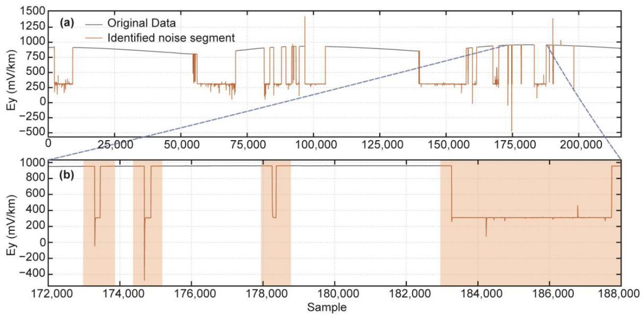
Figure 9 presents the Transformer-based identification results for strong interference in the observed Ey time series. As shown in Figure 9a, the field MT data contain various types of non-stationary interference, including long-duration step-like disturbances, impulsive spikes, and localized abnormal fluctuations. Compared with the synthetic experiments, the interference characteristics are more complex because multiple types of noise coexist in the observed data. The Transformer model accurately identifies the abnormal segments with different durations and amplitudes, demonstrating its capability to capture complex temporal patterns in real MT observations. An enlarged view is shown in Figure 9b, where the detected interference segments are highlighted. Both long-duration step-like disturbances and short impulsive anomalies are effectively identified, providing reliable noise localization for the subsequent signal reconstruction process.
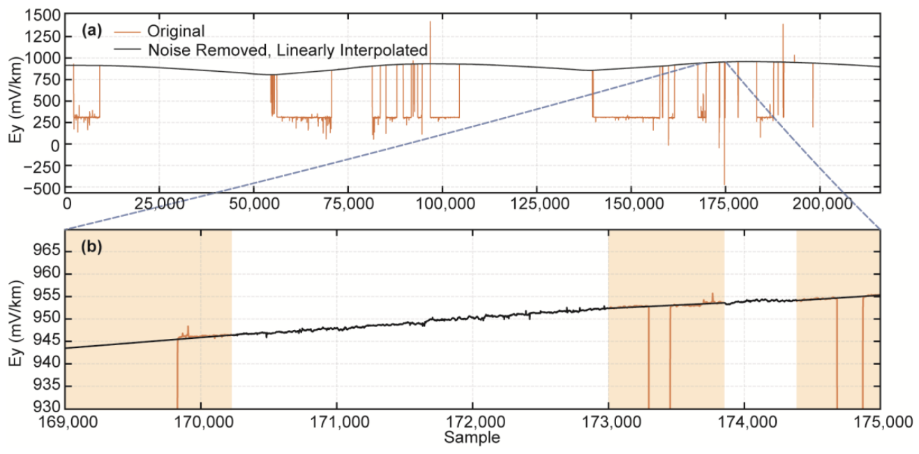
Based on the identified interference locations, the abnormal segments were removed and the missing intervals were reconstructed using linear interpolation, as shown in Figure 10. Figure 10a compares the original and reconstructed Ey time series, while Figure 10b provides an enlarged view of the reconstructed interval. After removing the detected interference, the reconstructed signal effectively eliminates the large-amplitude distortions caused by strong cultural noise while preserving the continuity and long-term variation trend of the original MT signal. These preprocessing results provide reliable input for subsequent PSO-VMD and random noise suppression.
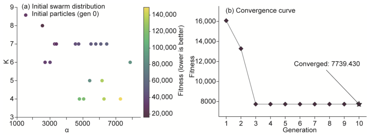
Before VMD, the number of modes K and the penalty factor α were adaptively optimized using the PSO algorithm to improve the decomposition performance of the field MT signal. As shown in Figure 11a, 18 particles were randomly initialized within the search space, and an iterative optimization process was then performed. Figure 11b shows that the optimal fitness value decreased rapidly during the initial iterations and stabilized after approximately three iterations, ultimately converging at 7739.430. The corresponding optimal parameters were K = 9 and α = 2000 . These optimized parameters were subsequently adopted for the subsequent VMD and random noise suppression of the field Ey signal.
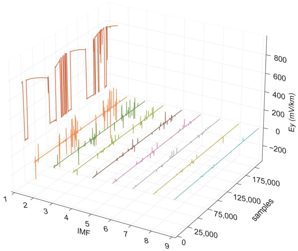
The PSO-optimized VMD method was further applied to the observed Ey signal for adaptive modal decomposition. As shown in Figure 12, the field signal was decomposed into nine intrinsic mode functions (IMFs) with distinct frequency characteristics. IMF1 mainly contains the low-frequency trend together with the dominant step-like interference observed in the field data, indicating that most of the large-scale non-stationary disturbances are concentrated in this mode. Therefore, IMF1 was regarded as the interference-dominated low-frequency mode and removed during the subsequent signal reconstruction. The remaining modes from IMF2 to IMF9 mainly reflect oscillatory components across different frequency bands. With increasing mode order, the characteristic frequency generally increases while the amplitude decreases, indicating that PSO-VMD can adaptively separate the complex non-stationary field signal into components at different frequency scales.
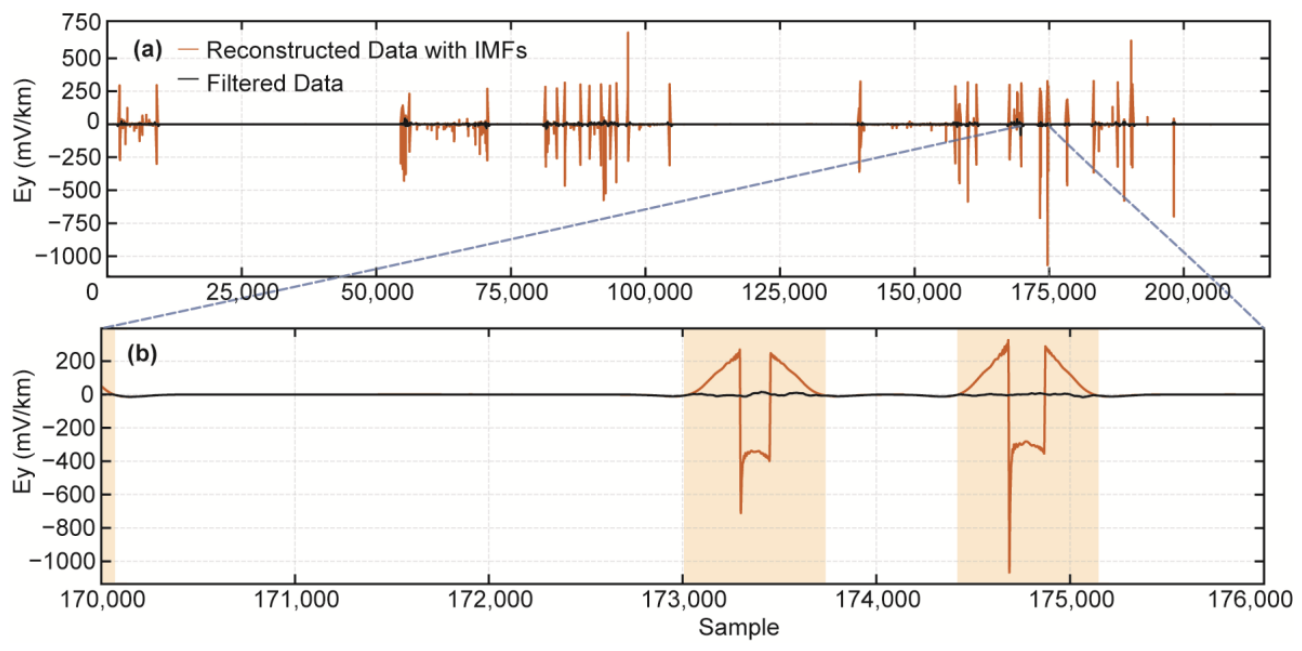
After removing the interference-dominated IMF1, the remaining modes (IMF2–IMF9) were reconstructed to obtain the high-frequency components containing useful signal information together with residual random noise. As shown in Figure 13a, the reconstructed high-frequency signal still exhibits noticeable high-frequency fluctuations in several previously identified interference intervals, indicating that some residual noise remains after modal reconstruction. A filtering operation was therefore applied to the reconstructed high-frequency components to suppress these fluctuations while preserving useful high-frequency information. Figure 13b presents an enlarged comparison of the signals before and after filtering. This selective reconstruction strategy suppresses residual random noise within the reconstructed intervals while avoiding unnecessary alterations to the uncontaminated portions of the field MT signal.
After obtaining the filtered high-frequency components from the reconstructed IMF2–IMF9 modes (Figure 13), these components were selectively superimposed on the linearly interpolated signal obtained after Transformer-based interference identification and removal (Figure 10) to generate the final denoised field MT signal (Figure 14). Specifically, the filtered high-frequency components were added only to the intervals where the strong interference had been removed and reconstructed using linear interpolation, whereas the original observed MT signal outside these reconstructed intervals was preserved without any modification. Consequently, the proposed reconstruction strategy restores interference-contaminated intervals while maintaining the original waveform characteristics of the uncontaminated portions of the field MT signal.
As illustrated in Figure 14a, the proposed method effectively suppresses large-amplitude step-like interference and localized abnormal fluctuations in the field MT signal while maintaining the overall temporal variation trend. Figure 14b presents an enlarged comparison within a representative interference interval. The reconstructed signal effectively restores waveform continuity after removal of the strong interference and suppresses residual random fluctuations without introducing noticeable distortion into the surrounding uncontaminated signal. These results demonstrate that the proposed local reconstruction strategy successfully reconstructs the interference-contaminated intervals while preserving the original characteristics of the uncontaminated portions of the field MT signal.
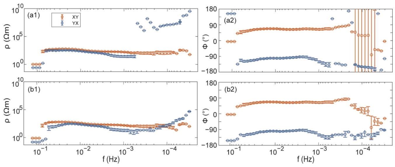
We further employed the RRMC algorithm [62] to estimate impedance tensors from both the original observed and denoised data. Figure 15 shows the apparent resistivity and impedance phase curves derived from the original observed and denoised data. The results show that the apparent resistivity curve of the yx mode derived from the observed data is severely distorted at periods >4000 s, while the corresponding impedance phase approaches 180 at longer periods (Figure 15(a1,a2)). After denoising, the distorted response curves are substantially corrected, with both the anomalous apparent resistivity and out-of-quadrant phase values of the yx mode returning to more reasonable values (Figure 15(b1,b2)), demonstrating that the proposed method can effectively improve the quality and stability of field MT transfer functions. Additionally, the xy modes derived from both the original and denoised data exhibit out-of-quadrant phases at periods greater than 9000s, which are likely associated with electrical anisotropy, galvanic distortion, and/or local 3D conductive bodies [63], rather than with typical background EM noise. Furthermore, although the xy phase values were not substantially altered by the denoising procedure, the error bars were significantly reduced (Figure 15(b2)).

4. Conclusions

To address the contamination of MT time series by strong cultural interference and random noise in complex observation environments, we developed a joint denoising framework that combines Transformer-based interference identification with PSO-optimized VMD. The method was evaluated using both synthetic and field MT data. The main conclusions are as follows:
  • The Transformer effectively identifies strong-interference noise segments in MT time series, including step-like anomalies, impulsive peaks, and complex non-stationary disturbances. Removal of the identified segments followed by linear interpolation restores signal continuity and provides a reliable basis for subsequent signal denoising.
  • PSO adaptively optimizes the key VMD parameters, improving the decomposition performance and stability of VMD for complex non-stationary signals. Compared with empirical parameter selection, PSO-VMD more effectively separates low-frequency, interference-dominated components from useful higher-frequency components.
  • After removal of the interference-dominated mode, the remaining high-frequency components are further filtered to suppress random residual noise. The final reconstruction combines the filtered components with the linearly interpolated signal within the identified interference intervals, enabling coordinated suppression of strong interference and random noise while minimizing modifications to uncontaminated signal segments.
  • Synthetic data experiments show that the proposed method can effectively recover the temporal characteristics of contaminated MT time series, improves the signal-to-noise ratio, and enhances the accuracy and stability of apparent resistivity and impedance phase estimates. Field data experiments further demonstrate its effectiveness under complex real-world noise conditions, resulting in more reliable MT response estimation.
Overall, the proposed Transformer–PSO-VMD framework integrates the strengths of deep learning for localized interference identification with the adaptive decomposition capability of VMD, providing an effective approach for robust MT data processing under complex noise conditions.
However, some limitations remain. The performance of the Transformer model depends on the quality and diversity of the training data and may degrade when field data contain previously unseen interference patterns. Improving model generalization through more diverse training datasets and domain-adaptation strategies is therefore an important direction for future work. In addition, the PSO-VMD optimization process introduces an additional computational cost, which may limit processing efficiency for long-duration or large-scale MT datasets.

Supplementary Materials

The following supporting information can be downloaded at: https://www.mdpi.com/article/10.3390/app16188931/s1. Supplementary Text S1. PSO-VMD optimization process for the synthetic dataset. Supplementary Text S2. PSO-VMD optimization process for the field dataset.

Author Contributions

Conceptualization, S.L., Y.T. and C.X.; methodology, S.L., Y.T. and C.X.; software, S.L. and Y.T.; writing—original draft preparation, S.L., Y.T. and C.X.; writing—review and editing, S.L. and C.X.; visualization, S.L.; supervision, C.X.; project administration, C.X.; funding acquisition, C.X. All authors have read and agreed to the published version of the manuscript.

Funding

This research was funded by the Deep Earth Probe and Mineral Resources Exploration–National Science and Technology Major Project, grant number 2024ZD1000403, and the National Natural Science Foundation of China, grant numbers 42474111 and 42074083.

Institutional Review Board Statement

Not applicable.

Informed Consent Statement

Not applicable.

Data Availability Statement

The datasets generated during the current study are publicly available in the Zenodo repository: https://doi.org/10.5281/zenodo.21739599.

Acknowledgments

We used the high-performance computing facilities at China University of Geosciences (Beijing) for data processing. We used the EMTF-FCU v4.0 developed by Gary D. Egbert and collaborators. We are grateful to the developers for making these codes available to the community.

Conflicts of Interest

The authors declare no conflicts of interest.

References

  1. Berdichevsky, M.N.; Dmitriev, V.I. Models and Methods of Magnetotellurics; Springer: Berlin/Heidelberg, Germany, 2008. [Google Scholar]
  2. Chave, A.D.; Thomson, D.J. Some Comments on Magnetotelluric Response Function Estimation. J. Geophys. Res. 1989, 94, 14215–14225. [Google Scholar] [CrossRef] [Scilit]
  3. Egbert, G.D. Robust Multiple-Station Magnetotelluric Data Processing. Geophys. J. Int. 1997, 130, 475–496. [Google Scholar] [CrossRef] [Scilit]
  4. Egbert, G.D.; Booker, J.R. Robust Estimation of Geomagnetic Transfer Functions. Geophys. J. Int. 1986, 87, 173–194. [Google Scholar] [CrossRef] [Scilit]
  5. Gamble, T.D.; Goubau, W.M.; Clarke, J. Magnetotellurics with a remote magnetic reference. Geophysics 1979, 44, 53–68. [Google Scholar] [CrossRef] [Scilit]
  6. Goubau, W.M.; Gamble, T.D.; Clarke, J. Magnetotelluric data analysis; removal of bias. Geophysics 1978, 43, 1157–1166. [Google Scholar] [CrossRef] [Scilit]
  7. Jones, A.G.; Chave, A.D.; Egbert, G.; Auld, D.; Bahr, K. A comparison of techniques for magnetotelluric response function estimation. J. Geophys. Res. 1989, 94, 14201–14213. [Google Scholar] [CrossRef] [Scilit]
  8. Li, G.; Zhou, X.; Chen, C.; Xu, L.; Zhou, F.; Shi, F.; Tang, J. Multitype Geomagnetic Noise Removal via an Improved U-Net Deep Learning Network. IEEE Trans. Geosci. Remote Sens. 2023, 61, 5916512. [Google Scholar] [CrossRef] [Scilit]
  9. Li, J.; Liu, Y.; Tang, J.; Ma, F. Magnetotelluric noise suppression via convolutional neural network. Geophysics 2023, 88, WA361–WA375. [Google Scholar] [CrossRef] [Scilit]
  10. Li, J.; Liu, Y.; Tang, J.; Peng, Y.; Zhang, X.; Li, Y. Magnetotelluric data denoising method combining two deep-learning-based models. Geophysics 2023, 88, E13–E28. [Google Scholar] [CrossRef] [Scilit]
  11. Manoj, C.; Nagarajan, N. The Application of Artificial Neural Networks to Magnetotelluric Time-Series Analysis. Geophys. J. Int. 2003, 153, 409–423. [Google Scholar] [CrossRef] [Scilit]
  12. Smirnov, M.Y. Magnetotelluric Data Processing with a Robust Statistical Procedure Having a High Breakdown Point. Geophys. J. Int. 2003, 152, 1–7. [Google Scholar] [CrossRef] [Scilit]
  13. Chave, A.D.; Thomson, D.J. Bounded Influence Magnetotelluric Response Function Estimation. Geophys. J. Int. 2004, 157, 988–1006. [Google Scholar] [CrossRef] [Scilit]
  14. Larsen, J.C. Transfer functions: Smooth robust estimates by least-squares and remote reference methods. Geophys. J. Int. 1989, 99, 645–663. [Google Scholar] [CrossRef] [Scilit]
  15. Oettinger, G.; Haak, V.; Larsen, J.C. Noise reduction in magnetotelluric time-series with a new signal-noise separation method and its application to a field experiment in the Saxonian Granulite Massif. Geophys. J. Int. 2001, 146, 659–669. [Google Scholar] [CrossRef] [Scilit]
  16. Usui, Y.; Uyeshima, M.; Sakanaka, S.; Hashimoto, T.; Ichiki, M.; Kaida, T.; Yamaya, Y.; Ogawa, Y.; Masuda, M.; Akiyama, T. New robust remote reference estimator using robust multivariate linear regression. Geophys. J. Int. 2024, 238, 943–959. [Google Scholar] [CrossRef] [Scilit]
  17. Ogawa, H.; Asamori, K.; Negi, T.; Ueda, T. A Novel Method for Processing Noisy Magnetotelluric Data Based on Independence of Signal Sources and Continuity of Response Functions. J. Appl. Geophys. 2023, 213, 105012. [Google Scholar] [CrossRef] [Scilit]
  18. Sato, S.; Goto, T.-N.; Kasaya, T.; Ichihara, H. Method for Obtaining Response Functions from Noisy Magnetotelluric Data Using Frequency-Domain Independent Component Analysis. Geophysics 2021, 86, E21–E35. [Google Scholar] [CrossRef] [Scilit]
  19. Egbert, G.D. Processing and interpretation of electromagnetic induction array data. Surv. Geophys. 2002, 23, 207–249. [Google Scholar] [CrossRef] [Scilit]
  20. Smirnov, M.Y.; Egbert, G.D. Robust principal component analysis of electromagnetic arrays with missing Data. Geophys. J. Int. 2012, 190, 1423–1438. [Google Scholar] [CrossRef] [Scilit]
  21. Spagnolini, U. Time-domain estimation of MT impedance tensor. Geophysics 1994, 59, 712–721. [Google Scholar] [CrossRef] [Scilit]
  22. Santarato, G.; Spagnolini, U. Cancelling directional EM noise in magnetoteilurics1. Geophys. Prospect. 1995, 43, 605–621. [Google Scholar] [CrossRef] [Scilit]
  23. Cai, J.-H.; Tang, J.-T.; Hua, X.-R.; Gong, Y.-R. An analysis method for magnetotelluric data based on the Hilbert–Huang transform. Explor. Geophys. 2009, 40, 197–205. [Google Scholar] [CrossRef] [Scilit]
  24. Garcia, X.; Jones, A.G. Robust processing of magnetotelluric data in the AMT dead band using the continuous wavelet transform. Geophysics 2008, 73, F223–F234. [Google Scholar] [CrossRef] [Scilit]
  25. Elouaham, S.; Nassiri, B.; El Abbadi, R.; El Melhaoui, O.; Said, S.; El Khadiri, K.; Dliou, A.; Latif, R.; Dlimi, S.; Zougagh, H. Hybridization Denoising Method for EMG Signals Using EWT and EMD Techniques. IREA 2025, 13, 574. [Google Scholar] [CrossRef] [Scilit]
  26. Carbonari, R.; D’Auria, L.; Di Maio, R.; Petrillo, Z. Denoising of magnetotelluric signals by polarization analysis in the discrete wavelet domain. Comput. Geosci. 2017, 100, 135–141. [Google Scholar] [CrossRef] [Scilit]
  27. Kappler, K.N. A data variance technique for automated despiking of magnetotelluric data with a remote reference. Geophys. Prospect. 2012, 60, 179–191. [Google Scholar] [CrossRef] [Scilit]
  28. Tang, J.; Li, G.; Xiao, X.; Li, J.; Zhou, C.; Zhu, H.-J. Strong noise separation for magnetotelluric data based on a signal reconstruction algorithm of compressive sensing. Chin. J. Geophys. 2017, 60, 3642–3654. (In Chinese) [Google Scholar] [CrossRef]
  29. Chen, J.; Heincke, B.; Jegen, M.; Moorkamp, M. Using empirical mode decomposition to process marine magnetotelluric data. Geophys. J. Int. 2012, 190, 293–309. [Google Scholar] [CrossRef] [Scilit]
  30. Li, J.; Zhang, X.; Tang, J. Noise suppression for magnetotelluric using variational mode decomposition and detrended fluctuation analysis. J. Appl. Geophys. 2020, 180, 104127. [Google Scholar] [CrossRef] [Scilit]
  31. Guo, Z.; Han, J.; Liu, L.; Wu, Y.; Hou, J.; Gong, X. Reducing reliance on observation duration of magnetotelluric impedance estimation with an improved instantaneous spectrum-based method. IEEE Trans. Geosci. Remote Sens. 2024, 62, 5912715. [Google Scholar] [CrossRef] [Scilit]
  32. Dragomiretskiy, K.; Zosso, D. Variational Mode Decomposition. IEEE Trans. Signal Process. 2014, 62, 531–544. [Google Scholar] [CrossRef] [Scilit]
  33. Shang, Z.; Zhang, X.; Yan, S.; Zhang, K. Suppression of strong cultural noise in magnetotelluric signals using particle swarm optimization-optimized variational mode decomposition. Appl. Sci. 2024, 14, 11719. [Google Scholar] [CrossRef] [Scilit]
  34. Xue, J.; Shen, B. A novel swarm intelligence optimization approach: Sparrow search algorithm. Syst. Sci. Control Eng. 2020, 8, 22–34. [Google Scholar] [CrossRef] [Scilit]
  35. Zhong, C.; Li, G.; Meng, Z. Beluga whale optimization: A novel nature-inspired metaheuristic algorithm. Knowl. Based Syst. 2022, 251, 109215. [Google Scholar] [CrossRef] [Scilit]
  36. Wang, Z.; Liu, Y.; Du, J.; Wang, Z.; Shao, Q. De-noising magnetotelluric data using variational mode decomposition combined with mathematical morphology filtering and wavelet thresholding. J. Appl. Geophys. 2022, 204, 104751. [Google Scholar] [CrossRef] [Scilit]
  37. Dramsch, J.S. 70 years of machine learning in geoscience in review. Adv. Geophys. 2020, 61, 1–55. [Google Scholar] [CrossRef] [Scilit]
  38. Li, G.; Gu, X.; Chen, C.; Zhou, C.; Xiao, D.; Wan, W.; Cai, H. Low-frequency magnetotelluric data denoising using improved denoising convolutional neural network and gated recurrent unit. IEEE Trans. Geosci. Remote Sens. 2024, 62, 5909216. [Google Scholar] [CrossRef] [Scilit]
  39. Tian, Y.; Xie, C.; Wang, Y. Long short-term memory recurrent network architectures for electromagnetic field reconstruction based on underground observations. Atmosphere 2024, 15, 734. [Google Scholar] [CrossRef] [Scilit]
  40. Zhang, L.; Li, G.; Chen, H.; Tang, J.; Yang, G.; Yu, M.; Hu, Y.; Xu, J.; Sun, J. Identification and suppression of multicomponent noise in audio magnetotelluric data based on convolutional block attention module. IEEE Trans. Geosci. Remote Sens. 2024, 62, 5905515. [Google Scholar] [CrossRef] [Scilit]
  41. Vaswani, A.; Shazeer, N.; Parmar, N.; Uszkoreit, J.; Jones, L.; Gomez, A.N.; Kaiser, Ł.; Polosukhin, I. Attention is all you need. In Proceedings of the 31st International Conference on Neural Information Processing Systems (NIPS 2017), Long Beach, CA, USA, 4–9 December 2017; pp. 5998–6008. [Google Scholar]
  42. Feng, C.; Li, Y.; Wu, Y. A noise suppression method of marine magnetotelluric data using K-SVD dictionary learning. Chin. J. Geophys. 2022, 65, 1853–1865. (In Chinese) [Google Scholar] [CrossRef]
  43. Li, G.; Gu, X.; Ren, Z.; Wu, Q.; Liu, X.; Zhang, L.; Xiao, D.; Zhou, C. Deep learning optimized dictionary learning and its application in eliminating strong magnetotelluric noise. Minerals 2022, 12, 1012. [Google Scholar] [CrossRef] [Scilit]
  44. Li, J.; Peng, Y.; Tang, J.; Li, Y. Denoising of magnetotelluric data using K-SVD dictionary training. Geophys. Prospect. 2021, 69, 448–473. [Google Scholar] [CrossRef] [Scilit]
  45. Li, G.; Liu, X.; Tang, J.; Deng, J.; Hu, S.; Zhou, C.; Chen, C.; Tang, W. Improved Shift-Invariant Sparse Coding for Noise Attenuation of Magnetotelluric Data. Earth Planets Space 2020, 72, 45. [Google Scholar] [CrossRef] [Scilit]
  46. Li, G.; Wu, S.; Cai, H.; He, Z.; Liu, X.; Zhou, C.; Tang, J. IncepTCN: A new deep temporal convolutional network combined with dictionary learning for strong cultural noise elimination of controlled-source electromagnetic data. Geophysics 2023, 88, E107–E122. [Google Scholar] [CrossRef] [Scilit]
  47. Li, G.; Liu, X.; Tang, J.; Li, J.; Ren, Z.; Chen, C. De-noising low-frequency magnetotelluric data using mathematical morphology filtering and sparse representation. J. Appl. Geophys. 2020, 172, 103919. [Google Scholar] [CrossRef] [Scilit]
  48. Hahn, S.L. Hilbert Transforms in Signal Processing; Artech House: Norwood, MA, USA, 1996. [Google Scholar]
  49. Hestenes, M.R. Multiplier and gradient methods. J. Optim. Theory Appl. 1969, 4, 303–320. [Google Scholar] [CrossRef] [Scilit]
  50. Rockafellar, R.T. A dual approach to solving nonlinear programming problems by unconstrained optimization. Math. Program. 1973, 5, 354–373. [Google Scholar] [CrossRef] [Scilit]
  51. Li, J.; Zhang, X.; Cai, J. Suppression of strong interference for AMT using VMD and MP. Chin. J. Geophys. 2019, 62, 3866–3884. (In Chinese) [Google Scholar] [CrossRef]
  52. Kennedy, J.; Eberhart, R. Particle Swarm Optimization. In Proceedings of the IEEE International Conference on Neural Networks (ICNN’95), Perth, WA, Australia, 27 November–1 December 1995; Volume 4, pp. 1942–1948. [Google Scholar] [CrossRef] [Scilit]
  53. Marler, R.T.; Arora, J.S. The weighted sum method for multi-objective optimization: New insights. Struct. Multidiscip. Optim. 2010, 41, 853–862. [Google Scholar] [CrossRef] [Scilit]
  54. Yi, C.; Lv, Y.; Dang, Z. A Fault Diagnosis Scheme for Rolling Bearing Based on Particle Swarm Optimization in Variational Mode Decomposition. Shock Vib. 2016, 2016, 9372691. [Google Scholar] [CrossRef] [Scilit]
  55. Ataman, E.; Aatre, V.; Wong, K. Some statistical properties of median filters. IEEE Trans. Acoust. Speech Signal Process. 1981, 29, 1073–1075. [Google Scholar] [CrossRef] [Scilit]
  56. Brockwell, P.J. Autoregressive processes. WIREs Comput. Stat. 2011, 3, 316–331. [Google Scholar] [CrossRef] [Scilit]
  57. Luo, J.; Ying, K.; Bai, J. Savitzky–Golay smoothing and differentiation filter for even number data. Signal Process. 2005, 85, 1429–1434. [Google Scholar] [CrossRef] [Scilit]
  58. Savitzky, A.; Golay, M.J.E. Smoothing and Differentiation of Data by Simplified Least Squares Procedures. Anal. Chem. 1964, 36, 1627–1639. [Google Scholar] [CrossRef] [Scilit]
  59. Xu, J.; Wu, H.; Wang, J.; Long, M. Anomaly Transformer: Time Series Anomaly Detection with Association Discrepancy. In Proceedings of the International Conference on Learning Representations (ICLR 2022), Online, 25–29 April 2022. [Google Scholar]
  60. Kullback, S.; Leibler, R.A. On information and sufficiency. Ann. Math. Stat. 1951, 22, 79––86. [Google Scholar] [CrossRef] [Scilit]
  61. Egbert, G.D.; Kelbert, A.; Meqbel, N.M. Mod3DMT and EMTF: Free Software for MT Data Processing and Inversion. In Proceedings of the AGU Fall Meeting, New Orleans, LA, USA, 11–15 December 2017. Abstract NS44A-04. [Google Scholar]
  62. Sokolova, E.Y.; Varentsov, I.M.; EMTESZ Working Group. The RRMC Technique Fights Highly Coherent EM Noise. In Proceedings of the 21. Kolloquium “Elektromagnetische Tiefenforschung”, Holle, Germany, 3–7 October 2005; pp. 124–136. [Google Scholar]
  63. Piña-Varas, P.; Dentith, M. Magnetotelluric Data from the Southeastern Capricorn Orogen, Western Australia: An Example of Widespread out-of-Quadrant Phase Responses Associated with Strong 3-D Resistivity Contrasts. Geophys. J. Int. 2018, 212, 1022–1032. [Google Scholar] [CrossRef] [Scilit]
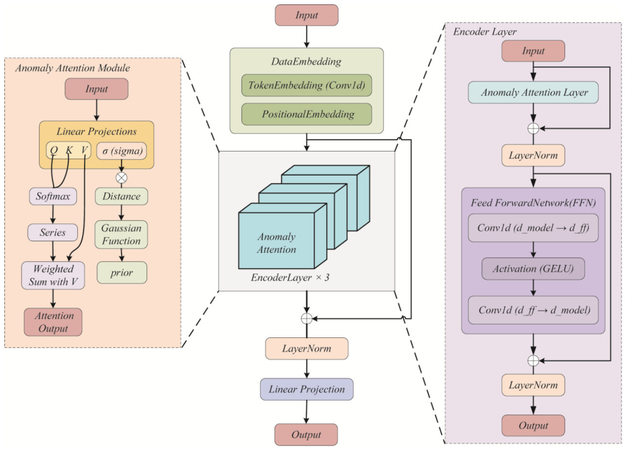
Figure 1. Structure of the Anomaly Transformer for time-series noise identification.
Applsci 16 08931 g001
Figure 2. Workflow of the proposed MT denoising method.
Applsci 16 08931 g002
Figure 3. Transformer-based interference noise detection, removal, and linear interpolation reconstruction. (a) Ex data contaminated by synthetic interference noise and (b) Ex signal after noise removal and linear interpolation. The shaded regions indicate the detected interference segments.
Applsci 16 08931 g003
Figure 4. The PSO parameter optimization process and convergence results. (a) Initial particle swarm distribution and (b) convergence curve of the optimal fitness value. The PSO-VMD optimization process is available in Supplementary Text S1.
Applsci 16 08931 g004
Figure 5. PSO-VMD results of the synthetic noisy Ex signal. Panels (ah) represent the eight decomposed intrinsic mode functions (IMFs), with IMF1 mainly representing a noise-dominated low-frequency component and IMF2–IMF8 representing signal components distributed across different frequency bands.
Applsci 16 08931 g005
Figure 6. Reconstruction results after removing the noise-dominated IMF1 and filtering the reconstructed high-frequency components. (a) Comparison of the clean, noisy, reconstructed (IMF2–IMF8 in Figure 5), and final filtered signals. (b) Comparison of the clean signal, reconstructed high-frequency signal, and filtered high-frequency signal.
Applsci 16 08931 g006
Figure 7. Final denoising results obtained by combining Transformer-based signal reconstruction and PSO-VMD-based random noise suppression. (a) Combination of the linearly interpolated signal obtained after Transformer-based interference removal (Figure 3b) and the filtered high-frequency components reconstructed from PSO-VMD (Figure 6b). (b) Comparison of the clean, noisy, and final denoised signals. (c) Enlarged comparison of the clean, noisy, and the final denoised signals within a representative interference interval.
Applsci 16 08931 g007
Figure 8. Apparent resistivity and impedance phase curves of the synthetic MT data for clean, noisy, and denoised data, respectively. Panels (a1,a2) show apparent resistivity and impedance phase derived from the clean data; panels (b1,b2) show the corresponding results for the noisy data, and panels (c1,c2) show those for the denoised data. The error bars (1.96 σ) were calculated from the standard errors of the impedance tensor components through first-order Taylor error propagation.
Applsci 16 08931 g008
Figure 9. Noisy data segment and Transformer-based interference identification for the Ey time series. (a) Original Ey signal with the detected strong interference noise segments and (b) enlarged view of the identified interference interval. The shaded regions indicate the detected strong interference segments.
Applsci 16 08931 g009
Figure 10. Reconstructed Ey signal after interference removal and linear interpolation. (a) Original and reconstructed Ey time series and (b) enlarged view of the reconstructed signal after linear interpolation. The shaded regions indicate the detected strong interference segments.
Applsci 16 08931 g010
Figure 11. The PSO parameter optimization and convergence results. (a) Initial particle swarm distribution and (b) convergence curve of the optimal fitness value. The PSO-VMD optimization process is available in Supplementary Text S2.
Applsci 16 08931 g011
Figure 12. PSO-VMD results of the field Ey signal. IMF1 mainly contains the low-frequency trend and interference-dominated components, whereas IMF2–IMF9 correspond to oscillatory components distributed across different frequency bands.
Applsci 16 08931 g012
Figure 13. Reconstruction and filtering results of the field Ey signal after removing IMF1. (a) Reconstructed high-frequency signal obtained from IMF2–IMF9 and the corresponding filtered signal. (b) Enlarged comparison of the reconstructed and filtered high-frequency signals. The shaded regions indicate the detected strong interference segments.
Applsci 16 08931 g013
Figure 14. Final denoising results of the field Ey time series obtained by combining Transformer-guided signal reconstruction and PSO-VMD-based random noise suppression. (a) Comparison of the original field and the final denoised signals. (b) Enlarged comparison of the original and denoised signals within a representative strong-interference interval. The shaded regions indicate the detected strong interference segments.
Applsci 16 08931 g014
Figure 15. Apparent resistivity and impedance phase curves derived from the field MT data before and after denoising. Panels (a1,a2) show the apparent resistivity and impedance phase derived from the original observed data, whereas panels (b1,b2) show the corresponding results derived from the denoised data. The error bars (1.96 σ) were computed from the standard errors of the impedance tensor components via error propagation using a first-order Taylor expansion.
Applsci 16 08931 g015
Table 1. Quantitative comparison of denoising performance in terms of SNR, RMSE, and PRD.
MethodSNR (dB)RMSE (mV/km)PRD (%)
EMD−22.89289.611395.60
EWT−21.33279.471382.76
Transformer−9.7435.92295.57
PSO-VMD−13.9439.83395.55
PSO-VMD-filter−10.2834.51323.56
Transformer–PSO-VMD-filter−5.6831.92192.37
Disclaimer/Publisher’s Note: The statements, opinions and data contained in all publications are solely those of the individual author(s) and contributor(s) and not of MDPI and/or the editor(s). MDPI and/or the editor(s) disclaim responsibility for any injury to people or property resulting from any ideas, methods, instructions or products referred to in the content.