Article

Seismic Reservoir Monitoring Using Wavelet Transforms and Machine Learning: A Double-Compression Approach


Center for Wave Phenomena, Department of Geophysics, Colorado School of Mines, Golden, CO 80401, USA
*
Authors to whom correspondence should be addressed.
Appl. Sci. 2026, 16(11), 5352; https://doi.org/10.3390/app16115352
Submission received: 24 April 2026 / Revised: 19 May 2026 / Accepted: 21 May 2026 / Published: 26 May 2026
(This article belongs to the Special Issue Applied Geophysical Imaging and Data Processing, 2nd Edition)

Abstract

Real-time seismic reservoir monitoring of geologic reservoirs requires both large-scale data management and efficient computational workflows. Addressing these challenges is facilitated by developing techniques capable of selectively capturing critical geologic features, thereby increasing computational efficiency and reducing data storage requirements. This paper proposes a double-compression framework integrating Haar wavelet transforms with machine learning (ML) for efficient multiparameter seismic inversion. First, Haar wavelet compression significantly reduces the dimensionality of the input elastic models, preserving essential geologic structures while limiting data volumes. Next, a convolutional neural network with the long short-term memory (CNN-LSTM) architecture, including dual encoders and multi-decoders, compresses seismic data into a latent space to generate a multi-scale P-wave velocity estimate. By leveraging transfer learning to speed up convergence and enhance prediction accuracy, we fine-tune the latent representation to estimate the P-to-S-wave velocity ratio and acoustic impedance at multiple resolution scales. Tests on the synthetic CO 2 -injection Kimberlina model show that wavelet-based compression—including detuning large-scale trends—minimizes artifacts in simulated wavefields and accelerates neural-network training. The results demonstrate that combining wavelet-based pre-compression for reservoir models with data-driven latent encodings for seismic data achieves high compression ratios, reduces computational costs, and maintains the fidelity of subsurface imaging. Compared with a redundant-decimation baseline, the proposed framework reduces network training time by approximately 70% and GPU memory usage by 33–73%, achieves a wavefield energy loss below 0.1% at a 16:1 model-dimension reduction, and produces multi-resolution predictions of V P , V P / V S , and acoustic impedance with normalized errors below 0.04 across all six wavelet decomposition levels. Thus, the double-compression framework enables robust and scalable seismic monitoring of elastic reservoir parameters.

1. Introduction

Real-time seismic reservoir monitoring is increasingly being used in hydrocarbon production [1,2], carbon capture utilization and storage (CCUS) [3], geothermal energy projects [4], and wastewater injection [5]. The corresponding growth of seismic data volumes acquired to monitor these activities is leading to new challenges in terms of how to preprocess, analyze, and store such data sets. For example, effective time-lapse (4D) seismic monitoring of CCUS activities requires repeatedly estimating multiple reservoir properties over long time periods. Physics-based algorithms such as elastic full-waveform inversion (E-FWI) are often used to estimate P-wave velocity ( V P ), S-wave velocity ( V S ), and density ( ρ ) [6,7,8,9]. However, performing E-FWI (especially in 3D) involves extensive preconditioning of low-frequency input data and mitigation of parameter trade-offs, as well as time-intensive iterative numerical optimization. Thus, even though physics-based E-FWI algorithms may generate high-quality seismic inversion results, they represent a labor-intensive and computationally complex undertaking that may not represent an optimal strategy for continuous long-term geophysical monitoring.
One of the main issues with E-FWI is that terabyte-size (or greater) seismic data volumes present significant data storage, transmission, and processing challenges. Two potential ways to facilitate the use of E-FWI for long-term seismic monitoring are to reduce the input data volume using now-standard compression techniques or to employ machine learning (ML) to generate lower-dimensional data representations. Data compression not only reduces storage requirements, but also enhances computational efficiency, which improves data transfer and analysis. Depending on the user-specified application and intended outcomes, data-compression algorithms may be lossy or lossless. Lossless algorithms are capable of recovering data of the same quality after compression and subsequent decompression, while lossy algorithms achieve higher compression rates by permitting certain quality degradation [10,11,12]. Higher compression ratios can lead to loss of fine details, which can be critical in 4D seismic analyses where small features can be geophysically significant [13,14].
Common data-compression techniques include the discrete cosine transform (DCT) and the discrete wavelet transform (DWT). Widely used in image compression (e.g., JPEG), the DCT transforms spatial-domain data into wavenumber components using a set of orthonormal cosine basis functions. In many images, the energy is mostly concentrated in the low-wavenumber components, allowing the DCT to represent the essential information with just a few large-magnitude coefficients. The remaining higher-wavenumber coefficients are often small and can be coarsely quantized or set to zero, leading to higher compression ratios. At large compression ratios, however, the DCT can introduce blocky artifacts, which degrade image quality [15].
Alternatively, the DWT decomposes signals into multiresolution representations, capturing dual-domain (i.e., spatial and wavenumber) information. This allows for more precise control over compression quality and for capturing localized image features. These features lead to improved compression performances without significant degradation in image quality [16]. Numerous wavelet bases (e.g., Haar, Daubechies, sym2, coiflets, bi-orthogonal) can be used to sparsely represent data and support multiresolution analysis (MRA). For example, the Haar wavelet transform (HWT) is effective in capturing highly localized model changes, which is essential for seismic inversion. Although the more traditional transforms listed above are also effective, they have some limitations, including significant computational cost, making them less suitable for large data sets and real-time applications [17].
Another class of compression techniques is based on machine learning (ML), recent advances in which have substantially improved data compression. Such methods as the K-means singular value decomposition (K-SVD) and dictionary learning (DL) capture elementary structures that sparsely represent signals [18,19]. DL has been used for seismic data compression [10,20], noise suppression [21], and data interpolation [22,23], among other applications. By expressing seismic signals as sparse combinations of learned atoms, DL achieves compression ratios superior to those of transform-based methods, while preserving essential features [24]. The main drawback of DL is the high computational cost incurred by learning and updating dictionaries, which can be prohibitive for large-scale seismic data sets [10].
Convolutional-neural-network (CNN) compression is another approach to learning compact image representations. Architectures like ComCNN and RecCNN are designed to preserve structural information while achieving high compression ratios and can outperform traditional codecs (e.g., JPEG) at low bit rates [25]. Recurrent neural networks, particularly those with long short-term memory (LSTM) units that capture temporal data dependencies [26], can be used for variable-rate image compression. Autoencoders, which compress and decompress data by encoding inputs to and decoding outputs from a lower-dimensional latent space, are suitable for lossy data compression and can achieve high compression ratios while maintaining acceptable accuracy [27]. Other options include generative adversarial networks (GANs), which can enhance image compression by producing high-quality reconstructions from compressed representations [28], and variational autoencoders designed to introduce stochasticity into the encoding process to model data uncertainty and improve compression performance [29].
The main advantage of ML methods is that they can adapt to specific data distributions, often resulting in higher compression efficiency compared to fixed transforms [28]. Neural networks (NNs) can be trained end-to-end to optimize both the compression ratio and reconstruction quality, thereby minimizing the total error [30]. Moreover, these deep-learning models can capture both spatial and spectral redundancies, which is particularly beneficial for multidimensional data, such as hyperspectral images, where joint spatial–spectral processing enhances compression performance [13]. However, training deep neural networks requires significant computational power and memory [17], which can be prohibitively expensive for large data sets or resource-constrained projects. Additionally, ML models typically need large amounts of labeled training data, which often are scarce or expensive to obtain.
Finally, Refs. [20,31] demonstrate that while multiresolution autoencoder approaches can achieve substantial compression at extremely low bit rates, their performance is highly sensitive to the characteristics of seismic data. In particular, noise and large inter-survey variability can significantly impair the preservation of essential information. Ref. [31] also reports that deep autoencoder methods are often competitive with traditional codecs (e.g., JPEG2000) in very low-bit rate conditions and typically require survey-specific training to produce acceptable reconstruction quality. Hence, despite the potential of ML models in seismic data compression, they may lack the robustness needed for broad generalization, suggesting that hybrid strategies might be more beneficial.
Although both wavelet- and ML-based compression have advantages and drawbacks, there is little research on how these two approaches could be combined to improve the effectiveness of data-compression processes. Here, we examine the advantages of applying ML techniques to sparser, distribution-specific representations of data sets that have already been compressed through (lossy or lossless) wavelet transforms. Such a “double-compression” approach could lead to further data reduction with controllable information loss that could be beneficial for time-lapse (4D) E-FWI and potentially offer a broadly applicable strategy for increasing compression efficiency in various data-intensive applications.
We examine this approach by taking advantage of multitask learning (MTL), transfer learning (TL), and data compression to train multi-CNNs (MCNNs) using multiscale reservoir attributes (usually estimated by 4D E-FWI) reconstructed by Haar wavelet transforms. Recently, ref. [32] demonstrated the efficacy of integrating MTL and TL for high-resolution reservoir monitoring, specifically for CO2 sequestration. Their approach used CNNs with multiple encoders and decoders to predict reservoir parameters from time-lapse seismic data. The authors initially trained the network to estimate P-wave velocity and subsequently applied transfer learning to fine-tune the model for predicting other reservoir parameters (i.e., S-wave velocity, density, and saturation). This methodology effectively addressed the challenge of training sample scarcity, while enhancing the accuracy of real-time fluid movement monitoring.
This work proposes a methodology in which MCNNs, initially trained to estimate a long-wavelength isotropic elastic model from multicomponent seismic data, are fine-tuned through TL to obtain higher-wavenumber model features. The challenge of managing large data sets in seismic 4D monitoring is addressed by employing a hierarchical multiresolution approach. This hierarchical strategy minimizes overall training costs while maintaining the accuracy needed for robust estimation of reservoir properties and ensuring scalability of the trained model to larger data sets. The novelty lies in coupling a Haar wavelet transform with a CNN-LSTM architecture in three ways: (1) the Haar transform decomposes the reservoir parameter into a hierarchy of resolution levels; (2) a multi-decoder architecture is connected one-to-one with these wavelet levels, ensuring that the learned latent code remains informative at each resolution level; and (3) transfer learning is applied across the resolution-specific networks.
The paper begins by discussing wavelet transforms, ML-based compression, the corresponding neural network architectures, and the proposed double-compression strategy. Then, we present the preconditioning of reservoir attributes, which is critical for stabilizing neural network training. Next, we quantify the trade-offs between compression efficiency and reconstruction accuracy and analyze how multiresolution reconstruction influences the fidelity of simulated seismic wavefields. Finally, we demonstrate the effectiveness of the proposed methodology using a realistic synthetic model of CO 2 injection into the Kimberlina reservoir in California, including a description of the data generation process, testing the effect of “detrending” the reservoir attributes on the neural network performance, testing the proposed double-compression framework against a more conventional approach, and a quantitative evaluation of the network’s ability to predict temporal changes in reservoir parameters.

2. Methodology

2.1. Wavelet-Transform Compression

The choice of wavelet depends on the information content and the required data resolution. Compared with the discrete cosine transform (DCT), the discrete wavelet transform (DWT) has significant advantages for higher-resolution images. The DCT remains the method of choice in block-based image codecs because it compresses signal energy into a few low-frequency coefficients and can be implemented with fast kernels [33]. Yet, the DCT operates on fixed blocks, so sharp interfaces that cross block boundaries give rise to ringing and blocking artifacts, which hamper reconstruction of thin layers. In contrast, the DWT decomposes data on a dyadic grid, with the coefficients describing features at successively coarser scales, while retaining exact spatial localization [34]. Hence, the DWT promotes a more uniform distribution of compression errors. Additionally, by decomposing the image into multiple frequency sub-bands, the DWT achieves stronger decorrelation of the pixel intensities (i.e., the coefficients in different sub-bands become less correlated with one another), which leads to more efficient encoding. Wavelet functions also provide localized support in both the spatial and wavenumber (frequency) domains, enabling the DWT to capture multiscale details with a small number of coefficients.
Defined by piecewise-constant basis functions, the HWT is straightforward to implement because it requires only nearest-neighbor differences and sums [16]. Those properties translate into accurate model reconstruction with negligible memory overhead, which is highly beneficial for on-the-fly processing in time-lapse (4D) reservoir monitoring [15,35]; exact preservation of block averages helps capture contrasts with just a few coefficients. In addition to computational efficiency and minimal memory requirements, the HWT decomposes data into large-scale (low wavenumber or frequency) and detailed (high wavenumber or frequency) components across multiple scales. This hierarchical decomposition captures both the coarse- and fine-scale details in the data.
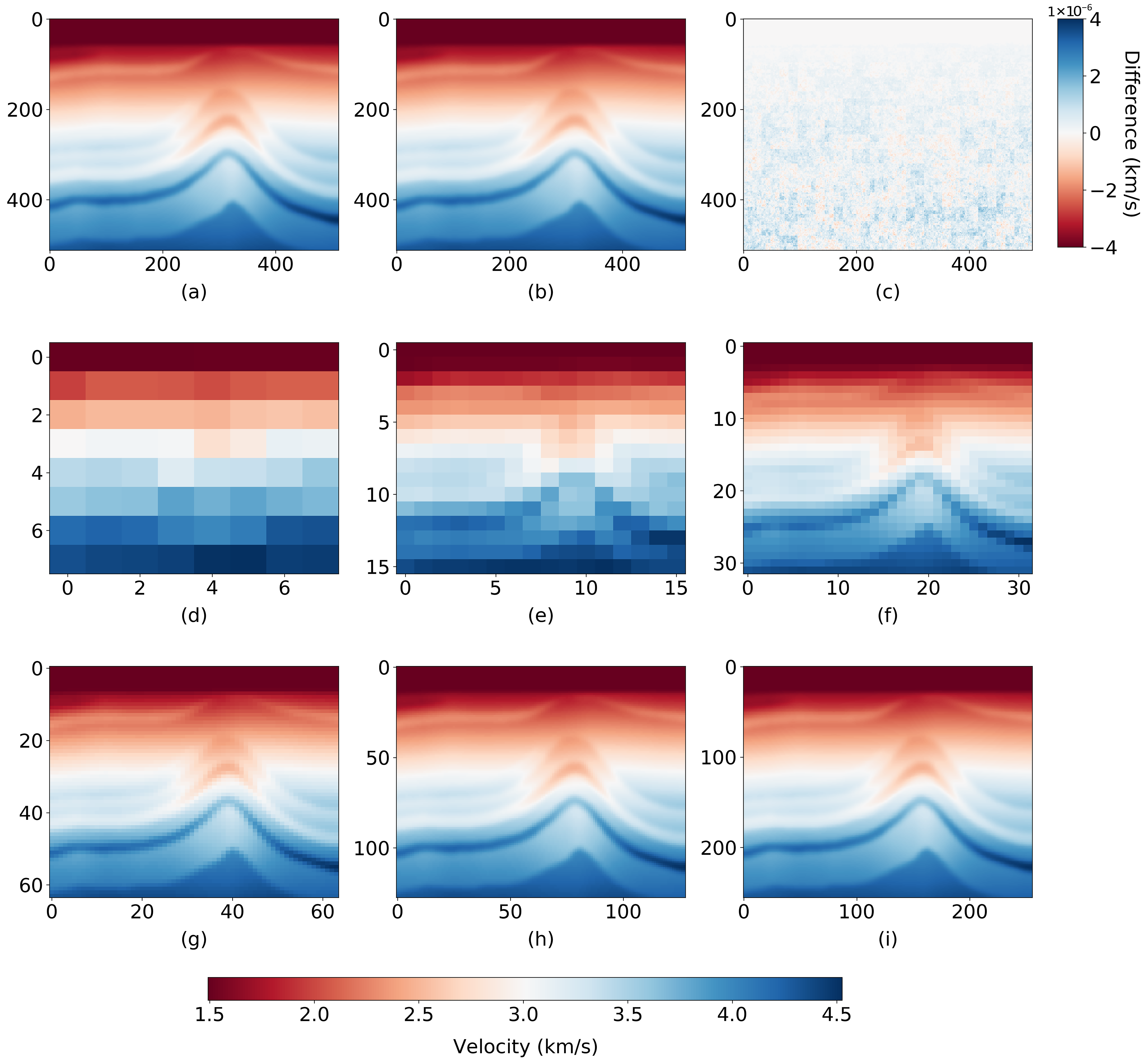
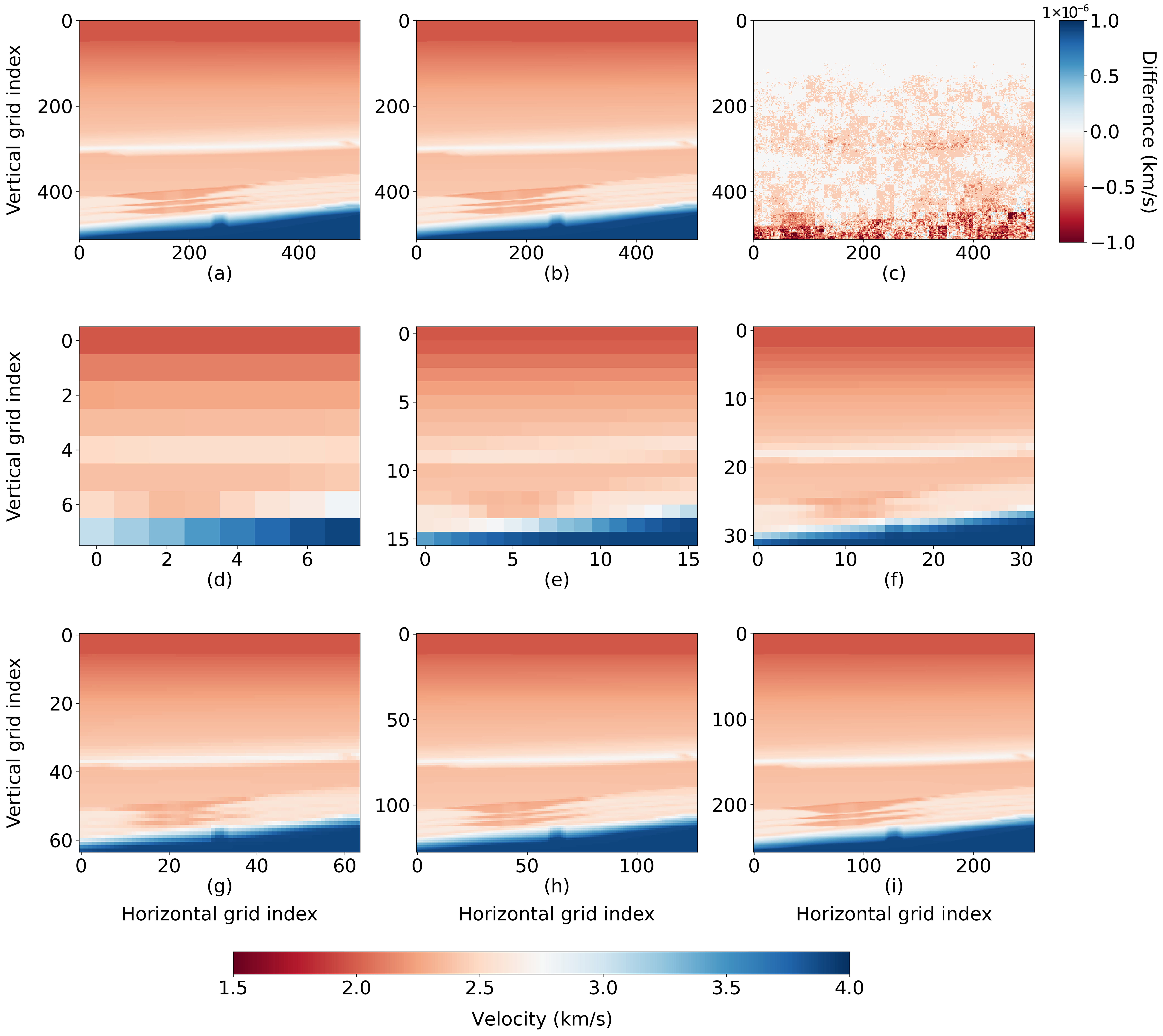
We perform tests for two different geologic scenarios using the Kimberlina CO 2 reservoir [36] and a section of the BP 2007 [37] model (Figure 1a and Figure 2a, respectively). Although the BP model was originally anisotropic (transversely isotropic with a tilted symmetry axis), here we retain only the isotropic model components. Each velocity model is subjected to a six-level wavelet decomposition, and the hierarchy of reconstructions is generated from the cumulative coefficient sets. The coarsest representation (L1) retains only the 8 × 8 approximation band; L2 adds the next-detail band to form a 16 × 16 grid. The next successive levels incorporate additional bands until reaching L6, which contains all coefficients and exactly reproduces the original model.
Here, we analyze how spatial velocity variations are influenced by the use of wavelet transforms [16]. For the Kimberlina model (Figure 1), the main features and the bottom layer remain continuous even at L3. The maximum error does not exceed 10 6 km / s , which corresponds to near floating-point accuracy. In the more structurally complex BP model (Figure 2), the anticline and low-velocity horizon are reproduced accurately; only the coarsest, 8 × 8 reconstruction exhibits visible staircasing.
Table 1 shows the data size and compression ratios for the 2D Kimberlina P-wave velocity model at various resolutions. The L3 reconstruction ( 32 × 32 ) cuts global memory storage from 420 MB to 0.8 MB (a 99.8 % reduction), while higher-order levels still save up to a minimum 87 % storage relative to the original model. The percentage reduction highlights the efficiency of wavelet transforms in capturing multiscale features, which allows for flexible trade-offs between data size and model resolution. The trade-offs between simple subsampling and wavelet-based compression (particularly in terms of computational cost) are discussed below.
We investigated five different wavelet families (Haar, Daubechies 2, and Biorthogonal 1.3, Sym2, Coif2) to examine the advantages of the HWT for image compression. Three wavelet transforms (Haar, Daubechies 2, and Biorthogonal 1.3) offer different trade-offs in terms of localization, smoothness, and filter length. Haar wavelets use piecewise-constant basis functions, while Daubechies 2 and Biorthogonal 1.3 employ more sophisticated filters that can provide smoother reconstructions. However, they also have larger filter lengths, which increases the computational overhead and may introduce artifacts. By comparing the wavelet families, we can determine which approach achieves the optimal balance between the compression ratio, computational cost, and reconstructed velocity model accuracy.
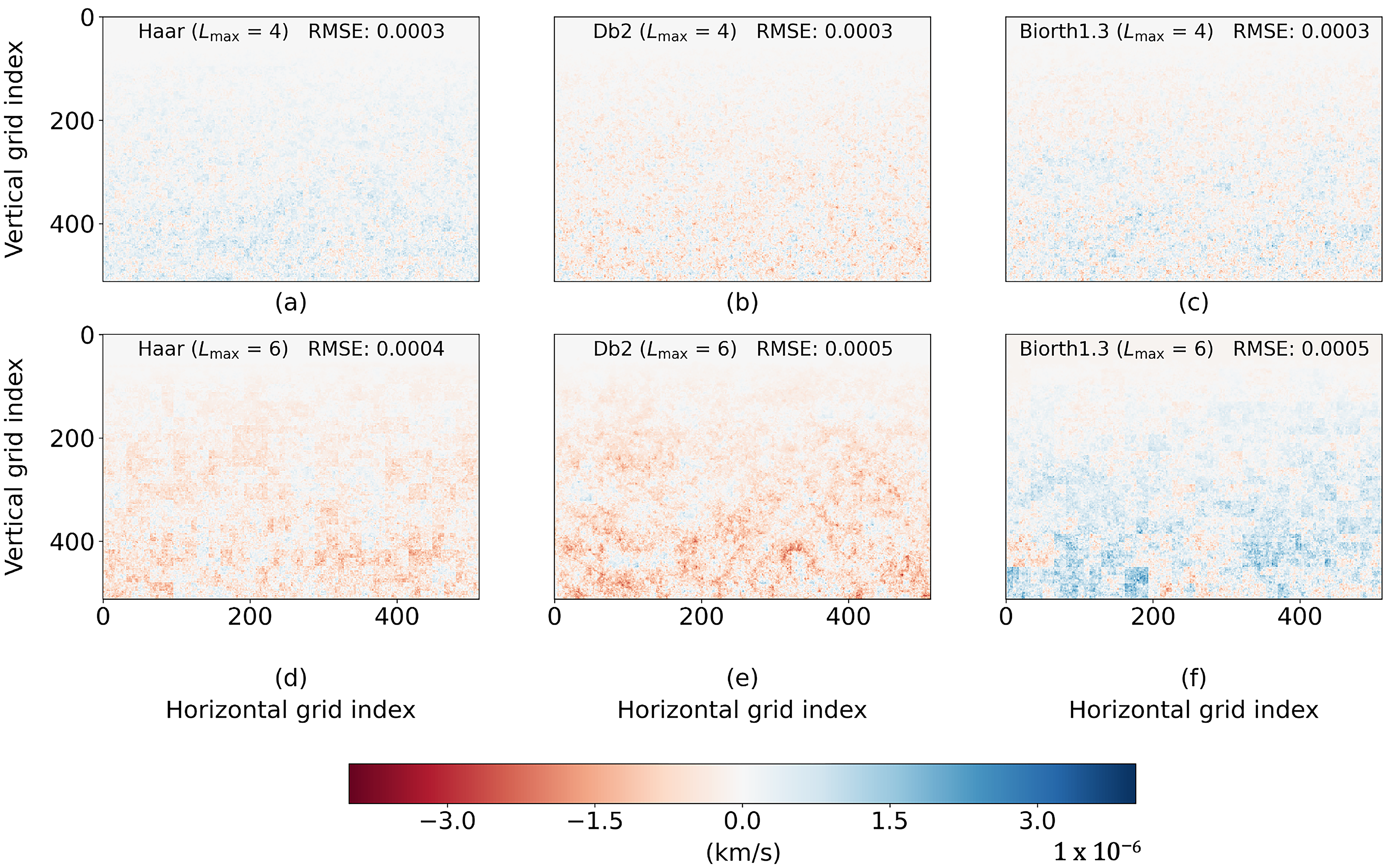
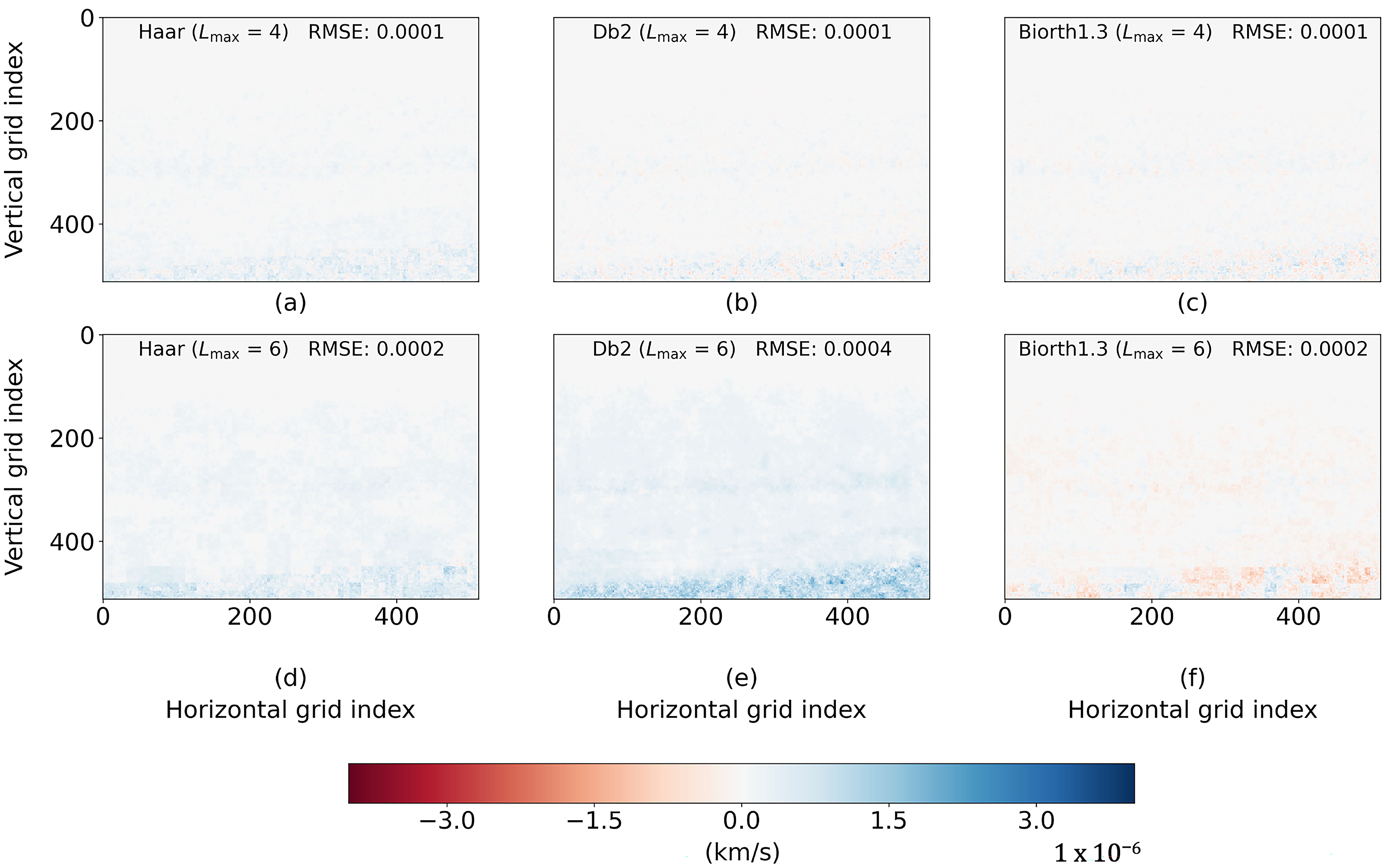
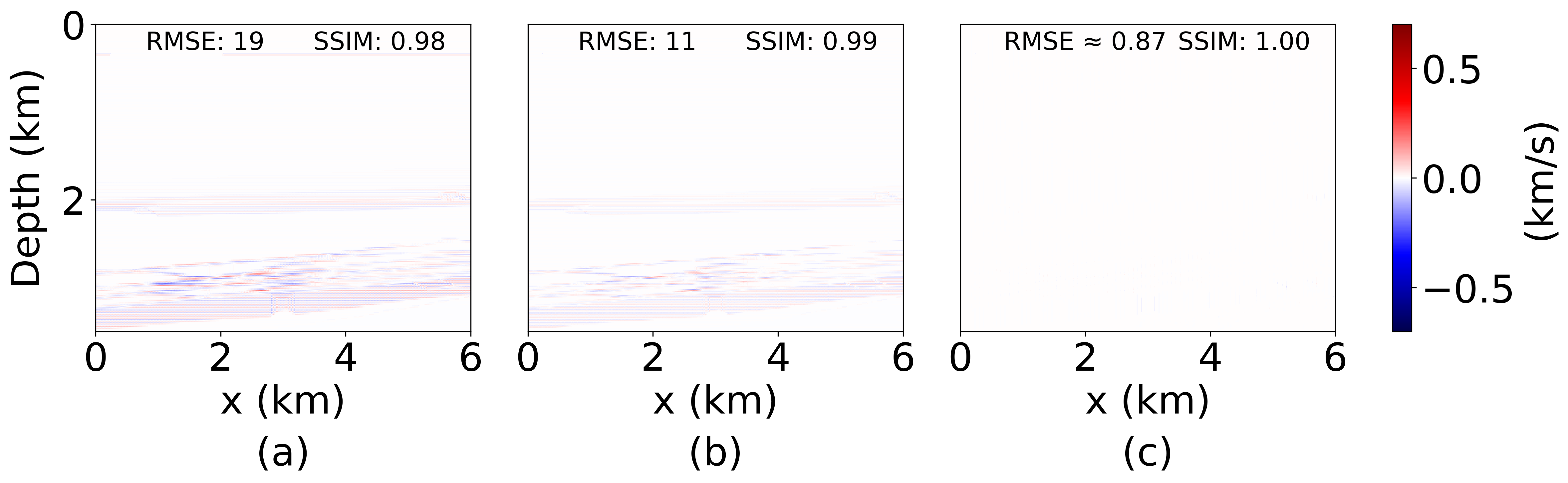
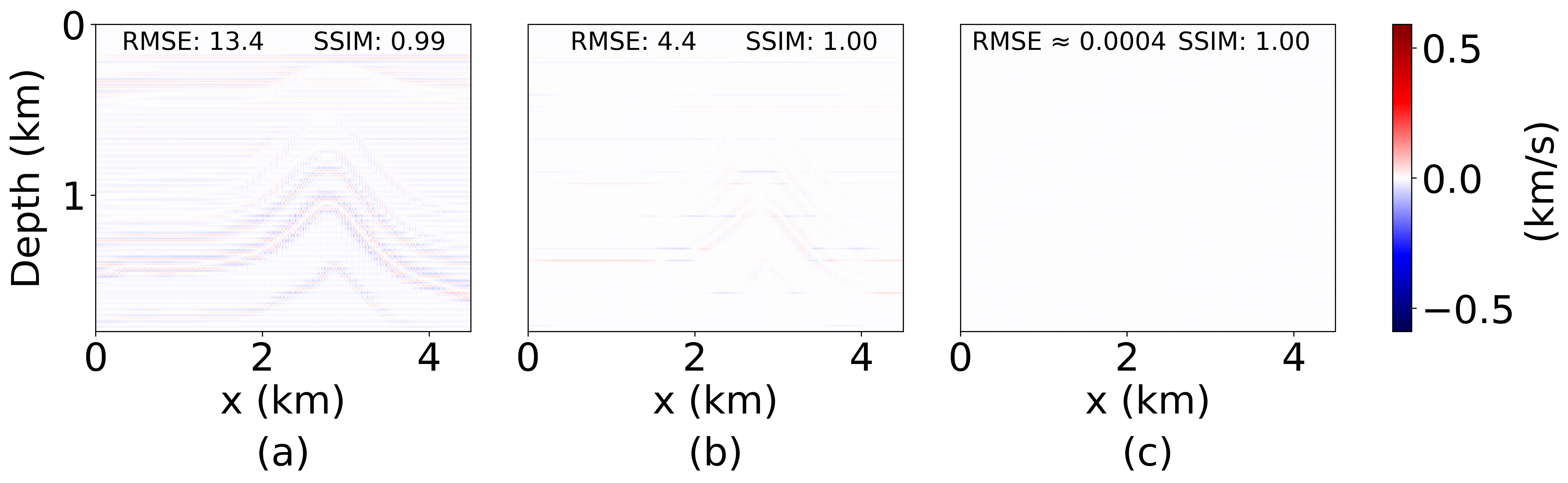
Figure 3 and Figure 4 illustrate the reconstruction accuracy of our wavelet-based compression for the Kimberlina and BP models, respectively. We compare the difference between the original velocity models and their wavelet-reconstructed counterparts for two maximum decomposition levels (L4 and L6) and three wavelet choices. For the maximum decomposition level (L4), all three wavelets yield similar results. The HWT has a slightly lower root-mean-square error (RMSE) for the Kimberlina model (Figure 3a–c), which indicates that it better preserves critical geologic structures at this intermediate scale. For L6, the overall differences become more pronounced (especially for Daubechies 2), yet the HWT have the smallest RMSE for both velocity models. The Biorthogonal 1.3 transform also performs well, particularly in areas with relatively smooth velocity variations. Whereas all three wavelets can compress the data with similar effectiveness, the HWT yields the most accurate reconstructions (i.e., the lowest RMSE) at higher compression levels. These properties collectively make the DWT and, in particular, the HWT highly effective for compressing and reconstructing data without losing essential model features. This underscores the benefit of selecting wavelets that balance simplicity with strong localization properties, which helps retain key geologic features found within elastic models.
Figure 1 and Figure 2 show the partial reconstructions across all six accumulated levels (L1–L6). Table 1 lists the storage size and percentage reduction at every level (from 99.9% at L1 to 87.0% at L6, plus the redundantly decimated 88 × 150 baseline). Finally, Figure 3 and Figure 4 compare the reconstruction RMSE for five wavelet families at maximum decomposition levels, L = 4 and L = 6 . The piecewise-constant Haar basis preserves sharp velocity contrasts at thin-bed reflection interfaces, fault boundaries, and salt-edge boundaries because no smoothing is applied. The smoother Daubechies and Coiflet bases trade this preservation for spectral compactness and, consequently, introduce artifacts responsible for the observed energy loss.
The HWT allows for efficient dimensionality reduction, which speeds up training and inference runs [38] of the CNN-LSTM architecture. It provides a computationally efficient, multiresolution representation of the parameter fields and effectively discards less-relevant fine-scale details before the data are processed by the neural network. This multiresolution preprocessing shortens the CNN-LSTM training run time, reduces memory usage, and improves model generalization [13,39]. Ref. [40] analyzes wavelet-transform-based data compression and finds that the HWT yields the optimal compression ratio while maintaining signal quality. Hence, the HWT can ensure sufficient image quality with high compression ratios and reduce the data volume to promote efficient data transmission and storage [41].

2.2. Machine-Learning-Based Compression

In recent years, ML approaches have shown great potential for data compression in such fields as computer vision, remote sensing, and geophysics. Traditional data-compression methods often rely on explicitly engineered features and prior assumptions about statistical distributions. In contrast, ML-driven methods leverage deep neural networks to learn more compact, lower-dimensional representations that preserve essential information and result in more efficient and adaptive compression [42]. In seismic applications, such adaptive compression is particularly valuable due to the large data volumes generated by multicomponent recordings of particle displacement or particle velocity. These volumes contain information about critical, yet sometimes subtle geologic features necessary for accurate velocity model-building and reservoir characterization. Previous studies have shown that seismic inversion can significantly benefit from ML-based dimensionality reduction, which can allow for efficient extraction of reservoir properties from large seismic data sets [43,44,45,46]. Large data volumes make storage, transmission, and subsequent seismic processing increasingly challenging. By applying ML methods, one can produce a data-driven compression model that reduces dimensionality while retaining the most salient characteristics.

2.2.1. Network Architecture

The compression model relies on a dual-encoder architecture to handle the two-component input seismic data. Ref. [47] demonstrate how distinct encoders for audio and video inputs can effectively learn cross-modal representations, leading to superior predictive performance. Ref. [48] incorporate multiple encoders into a GAN framework to separately handle various seismic attributes, thereby improving the inversion for velocity, porosity, and lithology.
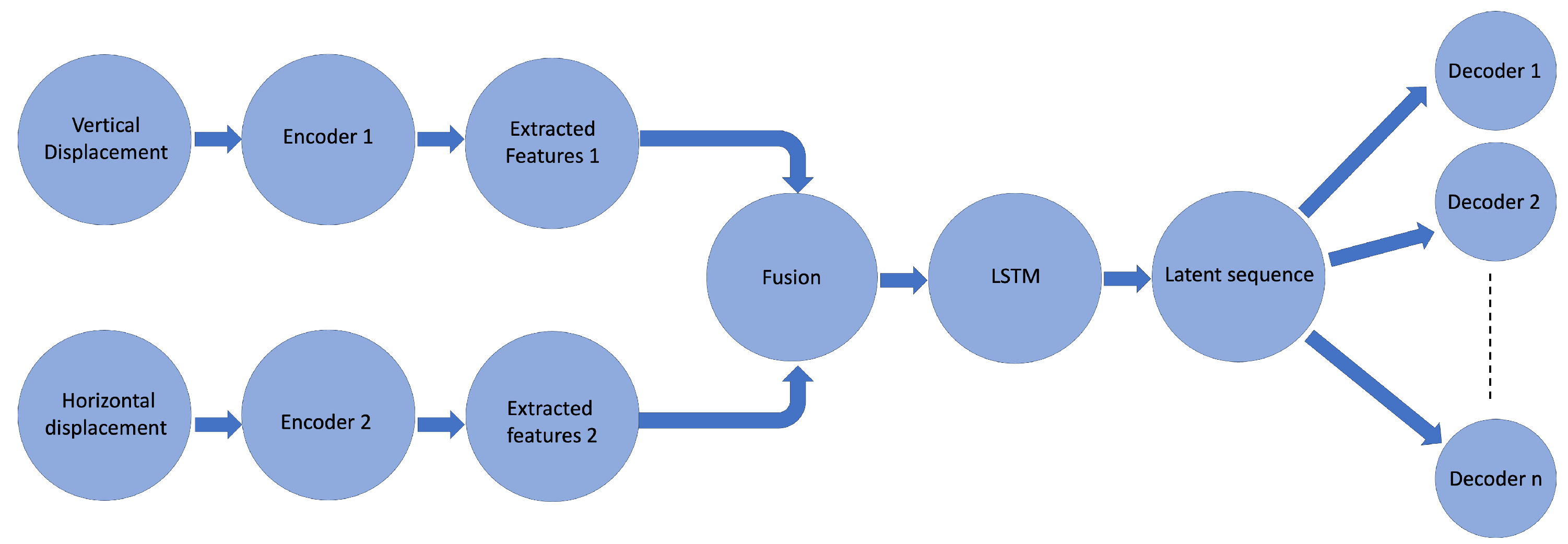
The starting point for our development is the framework proposed by [32] for estimating P- and S-wave velocities, density, and saturation from multicomponent seismic data. We employ a dual-encoder architecture, where each encoder is composed of five convolutional blocks. Detailed network hyperparameters, including the number of filters and kernel sizes, follow the specifications listed in Table 1 of [32]. Specifically, all hyperparameters used here (filter counts, kernel sizes, strides, padding, and latent-space size) are reported in Table 1 of [32]. The main architectural change in the present work is the introduction of the LSTM layer and the replacement of the single-decoder branch with a six-decoder branch (one per resolution level L 1 L 6 ) used to produce the multi-resolution outputs (Figure 5). Furthermore, we use the Gaussian Error Linear Unit (GELU) activation function because of its demonstrated ability to enhance generalization performance during transfer learning [32]. Each encoder layer is designed to learn progressively more abstract and compact representations of the input component by capturing spatio-temporal waveform patterns. Let E x ( · ) and E y ( · ) represent the encoders for the d x and d y arrays, respectively. Each encoder transforms the raw input sequences into a lower-dimensional latent representation,
[ z x z y ] = [ E x ( d x ) E y ( d y ) ] .
The outputs z x and z y are then combined into a single latent representation z using a fusion operator F (e.g., a fully connected or convolutional network). This fusion merges encoder feature maps, which reduces dimensionality and captures cross-component correlations critical for accurate seismic inversion:
z = F z x z y .
Because seismic data often exhibit significant temporal variations, we select a long-short-term-memory (LSTM) network [49] to process the fused latent representation z . The LSTM is chosen for its ability to capture long-term temporal dependencies, ensuring that the compressed representation is not only spatially compact but also temporally coherent. The LSTM operator transforms z into a temporally contextualized latent state h :
h = LSTM z .
This temporal embedding ensures that the compression retains the essential dynamic patterns of wave propagation, thus improving the ensuing decompression performance.
For multiscale (multiresolution) reservoir prediction, we develop a CNN with multiple decoders to estimate reservoir parameters from low to high frequencies (Figure 5). The decoder part consists of five deconvolution blocks designed to invert for reservoir parameters. By jointly training all the encoders, the LSTM NN, and the decoder, the system learns to produce a latent representation that captures spatio-temporal variations across multiple time scales. This approach allows the model to generalize temporal information for predictive analysis of future subsurface states beyond the simulation period represented in the training data. Such capabilities are critical for forward modeling and forecasting reservoir behavior in long-term CO2 injection projects, including predicting the migration characteristics of injected CO 2 plumes.

2.2.2. Network Optimization

The neural network is trained end-to-end using a hybrid L 1 - L 2 loss function denoted L vel designed for estimating velocity changes:
L vel = α V V ^ 1 + ( 1 α ) V V ^ 2 2 ,
where V and V ^ are the actual and predicted velocity models, respectively, and α is a “trade-off” weighting coefficient ( 0 α 1 ). The function L vel integrates the L 1 -norm and MSE (i.e., L 2 norm) contributions to increase robustness against outliers. In all experiments reported here we use α = 0.5 (an equal weighting of the L 1 and L 2 contributions), following the empirical choice validated in [32]. A finer-grained sensitivity analysis of α , including its interaction with the wavelet decomposition level, is the subject of a separate, dedicated study. We employ the Adam optimizer [50] during the training, along with such regularization methods as dropout and weight decay, to mitigate overfitting. These techniques help maintain generalization performance and promote convergence towards a solution suitable for forecasting velocity model changes due to CO 2 injection activities.

2.3. Double Compression

The synergy between the two compression stages can now be made explicit. The HWT acts as a deterministic, multi-resolution, and better sparsifying transform on the elastic parameter space because the Haar basis functions fully preserve block averages and have compact support while the HWT bounds the model-side reconstruction error and admits an analytical compression ratio per decomposition level (Section 2.1). The CNN–LSTM dual-encoder, in turn, acts as a learned, distribution-specific, lossy compressor on the seismic-data parameter space: it produces a non-linear latent code z that captures cross-component correlations between d x and d z and the temporal dependencies of wave propagation. The two stages are coupled at the supervision level—the targets that the CNN–LSTM is trained to predict are the wavelet-reconstructed velocity fields { V ( 0 ) , , V ( M ) } produced by Step 1.3 of Algorithm 1. Each decoder branch is therefore tied to a specific wavelet level, and the transfer-learning step lets the network first fit the low-frequency content captured at the coarse levels and then progressively refine the high-frequency detail represented at the finer levels. This coarse-to-fine, scale-by-scale training procedure is what distinguishes the present framework from a generic “transform → autoencoder” cascade.
Algorithm 1 Double compression
1:
Input
Reservoir parameter V
Seismic displacement components: vertical D z and horizontal D x
Low-level Haar decomposition level: L = 4
Maximum Haar decomposition level: M ( >L ) = 6
Neural network architectures: Dual Encoders, LSTM, multiple decoders
Neural networks: CNN 1 and CNN 2
2:
Step 1: Haar wavelet decomposition and partial (accumulated) reconstructions
1.1. Decompose the original velocity model V via Haar transform to obtain M levels of wavelet coefficients.
1.2. For k = 0 , M :
Accumulate all wavelet coefficients up to level k.
Perform inverse Haar transform to obtain the partial reconstruction V ( k ) .
  • (e.g., V ( 0 ) uses only level 0 coefficients; V ( 1 ) uses levels 0 + 1)
1.3. Generate set { V ( 0 ) , V ( 1 ) , , V ( M ) } , where V ( M ) is the full reconstruction of V .
3:
Step 2: Feature extraction from seismic data
2.1. Input vertical displacement d z into Encoder 1 to obtain feature vector f z .
2.2. Input horizontal displacement d x into Encoder 2 to obtain feature vector f x .
2.3. Concatenate f z and f x to form fused feature f concat yielding latent representation z .
2.4. Pass f concat through an LSTM layer to capture temporal variations.
4:
Step 3: CNN 1 training for the first four levels
3.1. Train CNN 1 to predict the partial reconstructions { V ^ ( 0 ) , V ^ ( 1 ) , , V ^ ( L 1 ) } from the latent representation z .
   i.e., minimize the MSE between V ^ ( k ) and the ground-truth V ( k ) for k { 0 , , L 1 } .
3.2. Let θ 1 denote the trained parameters of CNN 1 .
5:
Step 4: Fine-tuning CNN 2 for the remaining Levels
4.1. Initialize CNN 2 with the pretrained weights from CNN 1 (partial transfer of θ 1 ).
4.2. Train CNN 2 to predict the remaining partial reconstructions { V ^ ( L ) , , V ^ ( M ) } ,
   again by matching them to the corresponding ground-truth reconstructions { V ( L ) , , V ( M ) } .
4.3. Freeze the encoder layers ( E x , E y ) and fine-tune only the multi-resolution decoder branches corresponding to levels { L , , M } .
6:
Step 5: Final velocity reconstruction
5.1. The final predicted velocity model is V ^ ( M ) , which corresponds to the accumulated levels k = 0 M .
7:
Return:  V ^ ( M )
We first apply HWT-based compression to the input reservoir parameters to reduce their spatial dimensionality and facilitate faster and more memory-efficient CNN-LSTM training (Algorithm 1). Subsequently, the CNN further compresses the data into a latent space. The NN performs a learned nonlinear compression, tailoring its latent codes to the underlying data physics. This two-stage (double) compression leverages the complementary strengths of classic wavelet transforms and data-driven methods.
HWT-based compression reduces the input size and complexity before NN training, resulting in fewer trainable parameters, faster epoch calculation, and reduced GPU memory usage [28,51]. Such efficiency gains are crucial for facilitating large-scale 3D simulations and continuous field monitoring. The proposed methodology integrates HWT-based dimensionality reduction and CNN-LSTM latent representation to compress both reservoir models and seismic data. This double-compression approach reduces computational costs and memory footprint and makes it possible to reconstruct reservoir parameters with high accuracy and resolution. Through training on simulated long-term CO 2 injection data and testing on post-injection seismic data sets, we demonstrate that the synergy between wavelet transforms and data-driven latent encoding improves reservoir management and monitoring.

2.4. Reservoir Parameter Preprocessing

The distributions of target reservoir parameters in the training samples can strongly influence NN convergence properties and generalization performance [52,53]. When networks are trained on overly broad and poorly sampled parameter spaces, they experience difficulties learning relevant features without extensive regularization, which can result, for example, in overfitting in underrepresented regions. Ref. [54] demonstrates that adapting pretrained networks to handle computer-vision tasks with highly divergent or insufficiently sampled distributions degrades NN convergence and accuracy. In contrast, well-aligned and constrained data distributions can significantly reduce training time in natural language algorithms, while improving downstream performance, as reflected in transfer-learning surveys [55].
Geophysical parameter (e.g., velocity, density, or saturation) distributions often span a wide range of values, yet remain sparsely sampled. Studies in seismic reservoir monitoring and imaging confirm that reducing and/or better sampling these parameter spaces improves NN convergence [56]. By reducing parameter ranges (e.g., that of the S-wave velocity V S ), networks can avoid overextending into areas with insufficient training data [32]. This not only stabilizes the learning process, but also preserves computational resources by mitigating the need for exhaustive searches or extensive regularization. Overall, the importance of data- and parameter-space alignment for NNs underscores a fundamental principle in machine learning: well-constrained, representative distributions are key to efficiently achieving optimal training.
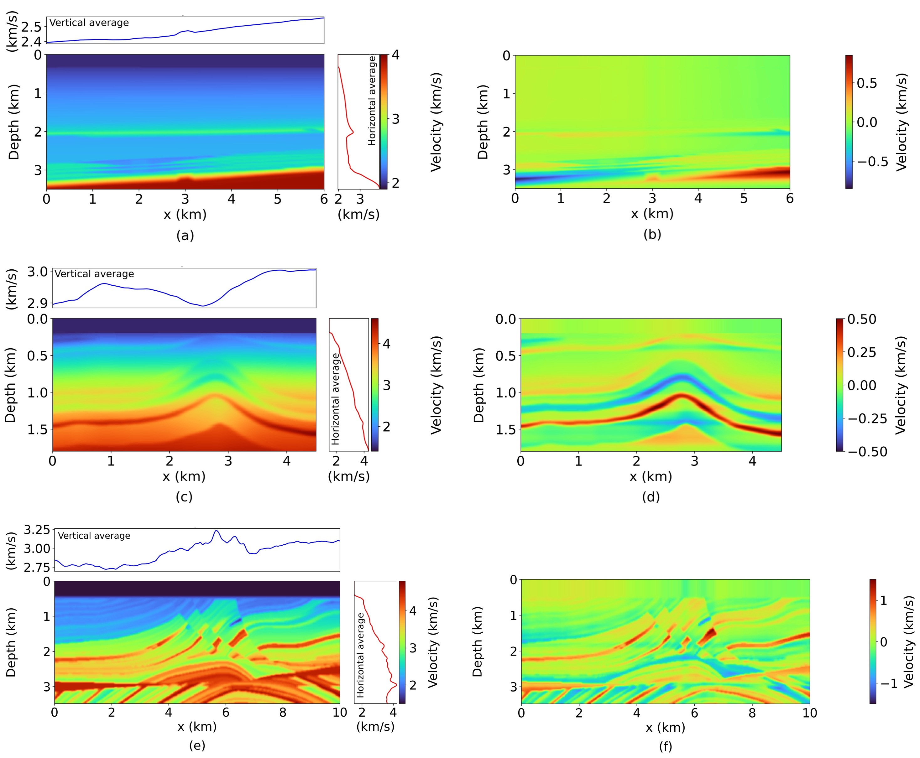
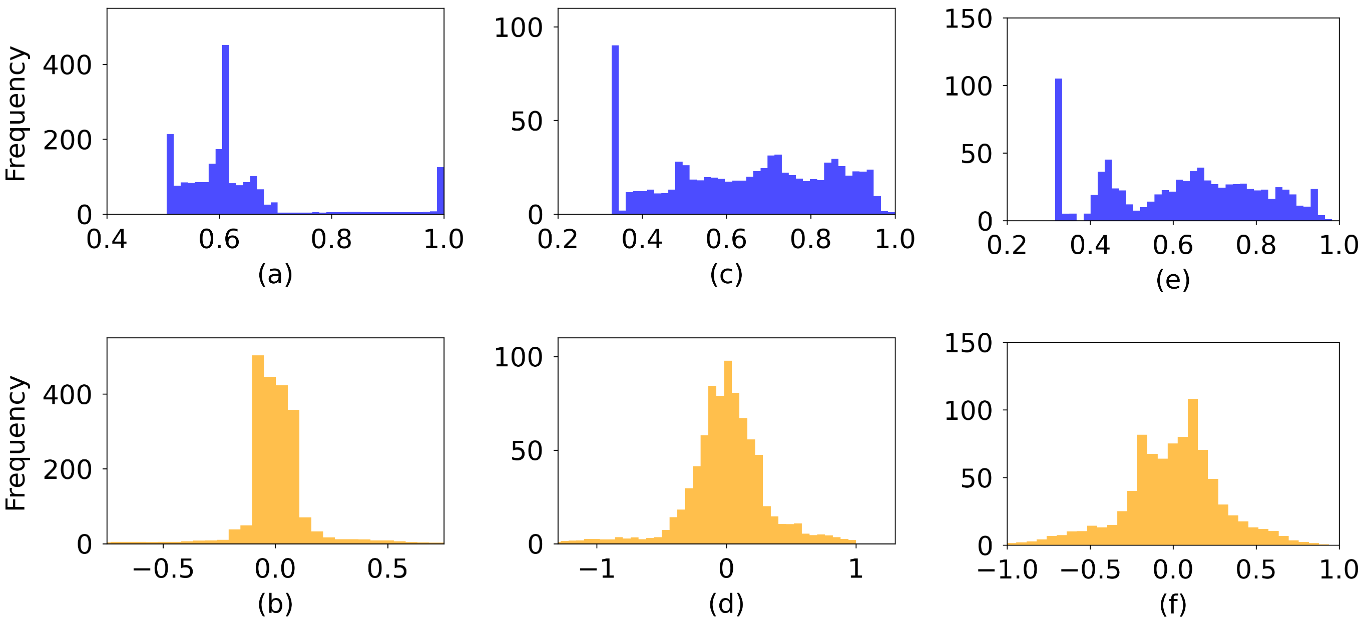
We investigate the removal of background P-wave velocity variations in three velocity models: Kimberlina, BP, and Marmousi. The one-dimensional (1D) vertical and horizontal mean velocity values for each model are subtracted from the original data (Figure 6). The histograms of such “detrended” models (Figure 7) confirm that they have a more narrow velocity range compared to those with uniform sampling. Consequently, the NN input has the potential for improved network convergence.

3. Wavelet-Based Compression Test

3.1. Compression Evaluation Metrics

To quantify the effects of wavelet-based compression on storage overhead and the reconstructed model accuracy, we integrate standard quantitative metrics with domain-specific performance tests. The compression ratio (the ratio of the original and compressed data sizes) quantifies algorithmic efficiency. Metrics such as signal-to-noise ratio (SNR), structural similarity index (SSIM), and root-mean-square error (RMSE) help evaluate the accuracy of the reconstructed signals [57]. Additionally, comparing the performance of downstream analyses (e.g., migration and inversion) using compressed versus uncompressed data can provide domain-specific validation [58]. We evaluate the accuracy of the velocity models reconstructed using wavelet decompositions at all levels, then at the first five levels, and at the first six levels. Because the HWT requires the input dimensions to be a power of two, we resize the original Kimberlina (350 × 600) and BP (174 × 180) models to be of dimension 512 × 512. We then resize all reconstructed models back to their original dimensions to compute the RMSE and structural similarity index (SSIM) (Figure 8 and Figure 9).

3.2. Wavefield Reconstruction Quantification

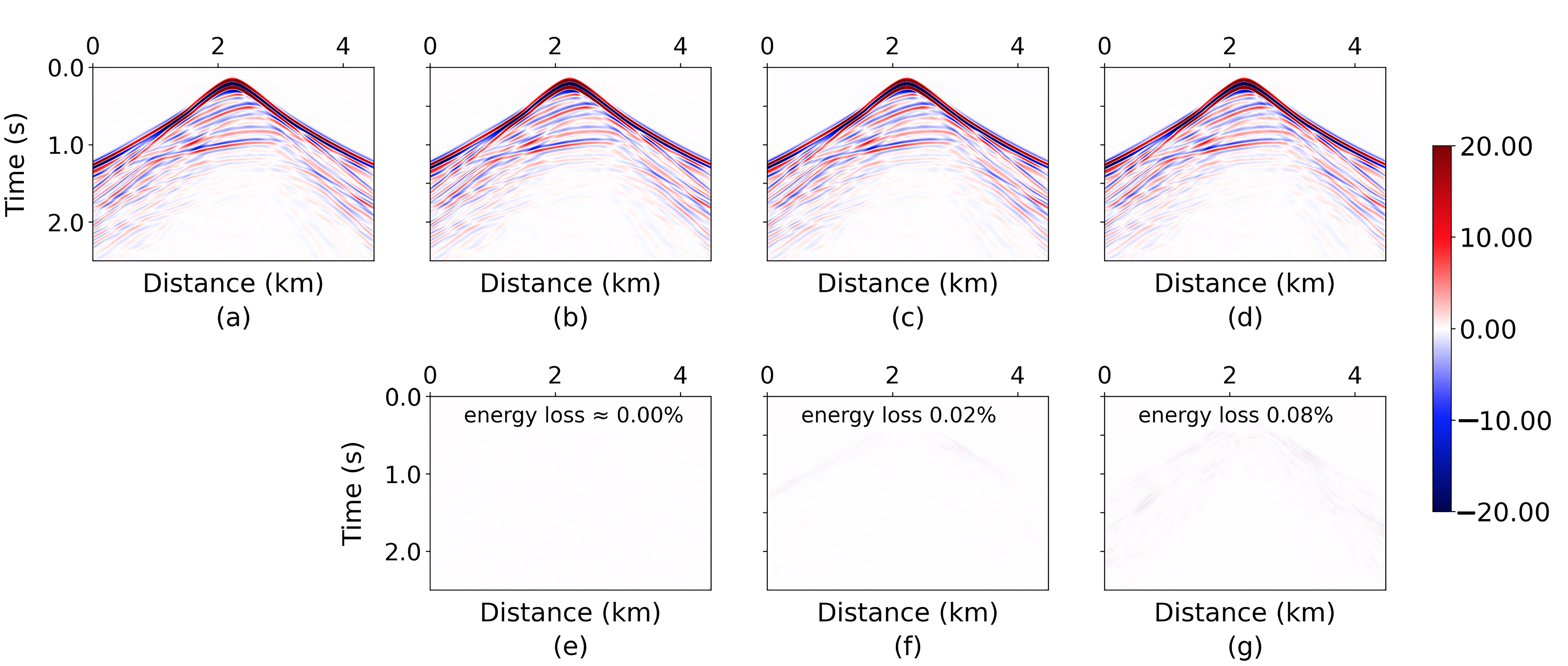
Here, we investigate how wavelet-based velocity-field reconstruction influences seismic data simulated for the BP and Kimberlina models. Our goal is to determine whether compressing and then reconstructing the model parameters (i.e., to grids of 128 × 128 , 256 × 256 , or 512 × 512 ) introduces artifacts significant enough to hamper reservoir characterization and/or seismic imaging. In particular, one needs to evaluate whether amplitude information in the simulated wavefield, which is essential for monitoring subsurface fluid migration, remains sufficiently accurate after compression. For the BP model, a source with a central frequency of 12 Hz is placed at location ( x , z ) = ( 2230 , 1 ) m . A total of 450 equally spaced (10 m interval) receivers are located at a depth of 210 m to record the wavefield. The simulated shots are used to assess the robustness of the HWT-reconstructed models.
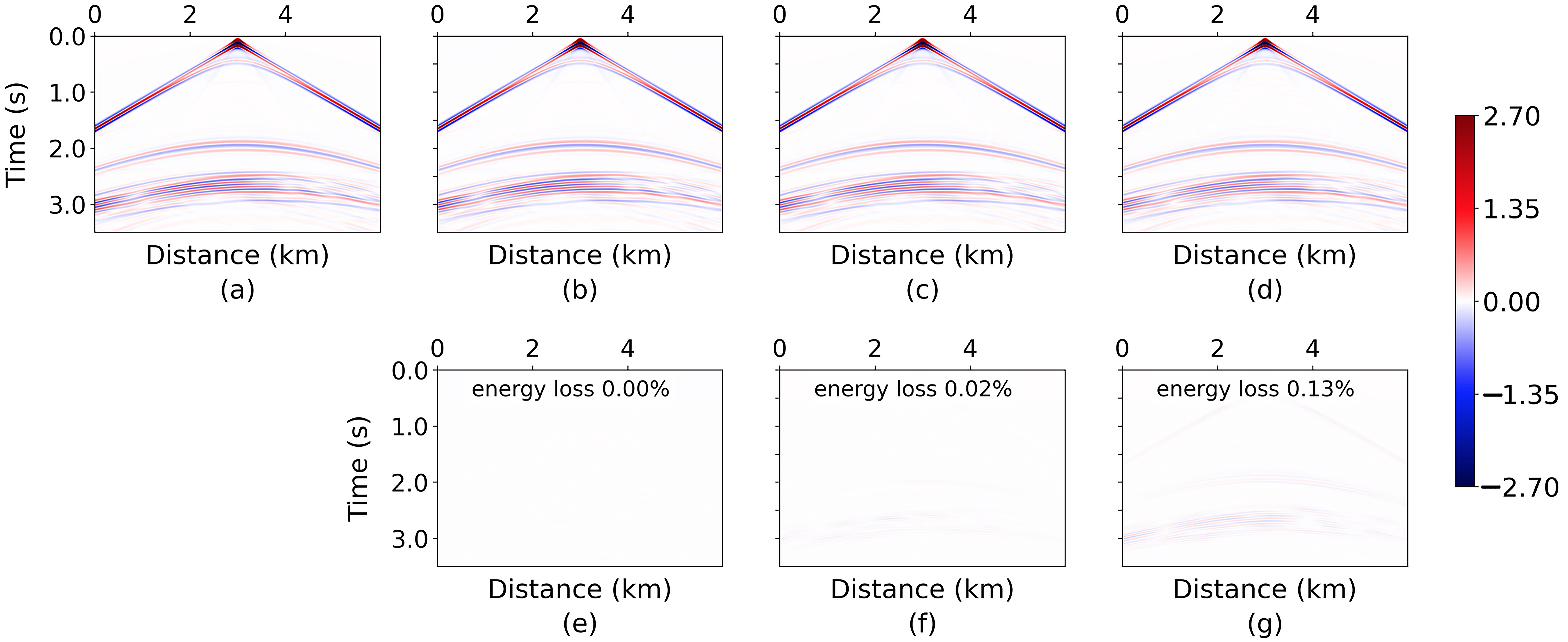
Figure 10 compares shot records generated for the original Kimberlina model with those reconstructed at three different grid resolutions. The Kimberlina model features several layers but exhibits longer-wavelength heterogeneity than the BP model. The results in Figure 10 and Table 2 (M2 columns) show that the HWT causes fewer distortions (artifacts) than the other wavelets, particularly for highly compressed grids (e.g., 128 × 128 ).
Figure 11 performs the same comparison for the BP model. To quantify the differences, we compute the total wavefield energy before and after reconstruction. Table 2 (M1 columns) presents the percentage energy loss for five wavelet transforms (Haar, Daubechies 2, Symlet 2, Biorthogonal 1.3, and Coiflet 2). While all transforms preserve most wavefield energy—even at coarser resolutions—the results indicate that the HWT consistently yields the lowest energy loss, likely because the underlying piecewise-constant basis functions more effectively capture sharp velocity contrasts. This is essential for accurately characterizing subsurface geologic structures, such as salt domes that disrupt continuous sedimentary layers or strong lateral velocity variations across fault planes. This outcome confirms the suitability of HWT for structurally complex models.
For both the Kimberlina and BP models, the difference panels highlight localized changes in the wavefield amplitudes or phases arising from the model compression. The HWT reconstructions introduce only minor artifacts largely confined to areas around sharp velocity boundaries.

4. Neural Network Test

4.1. Generating Training Labels

4.1.1. Reservoir Parameters

Empirical relationships between P-wave velocity, porosity, and permeability, validated by laboratory and field studies [59,60], can be used to approximate the time-varying CO 2 saturation. Following [32,61], we employ linear velocity-saturation correlations (see the latter’s Figure 10) to produce synthetic CO 2 saturation maps from the available well logs. The regression coefficients for these correlations are determined by analyzing sonic-log data from both injection and monitoring wells over multiple years, which helps constrain the velocity range for the training samples. Because these velocity-saturation relationships are calibrated for the Kimberlina model, their applicability to other reservoirs may be limited.
In constructing the training data set, we assume that E-FWI has provided an estimate of the pre-injection baseline velocity field, which is then perturbed within the reservoir to generate realistic “label” models for the network. As outlined in [32,61], CO 2 migration can be approximated by a depth-dependent transport-velocity function, yielding a total of 14,000 synthetic samples that contain the values of V P , V S , ρ , and CO 2 saturation. Of these, 12,000 models spanning 10 years after injection are reserved for training the V P -prediction network, while models corresponding to 12 years post-injection are used for testing. Subsequently, transfer learning [32] is employed to adapt the model trained on V P for predicting the V P / V S ratio and acoustic impedance.

4.1.2. Seismic Data

The proposed neural network is applied to a synthetic data set for the Kimberlina reservoir. The simulated CO 2 injection takes place in a saline reservoir overlain by six sand-shale layers, and the injected plume rises mainly due to buoyancy effects [62]. The data set spans multiple time snapshots that capture reservoir behavior over 20 years during and post injection [36]. To investigate how CO 2 migrates and causes 4D changes in subsurface properties, we select a 2D seismic line at x = 2100 m and generate synthetic seismic traces by solving the elastic wave equation with a finite-difference time-domain algorithm. We use a 10 Hz Ricker source wavelet and record both the vertical and horizontal displacement components. This modeling procedure is repeated at multiple time steps, generating a 4D seismic data set that captures the effects of temporal parameter changes associated with the injection process.

4.2. Reservoir Parameters Preconditioning Test

Building on the model preprocessing strategies discussed in the Section 2.4, we now explore whether removing the 1D background velocity variations from the Kimberlina model improves NN convergence and predictive accuracy. For this purpose, we compute the detrended (residual) V P models formed by subtracting the 1D vertical and horizontal means from the original velocity field. This “detrending” reduces the dynamic range and “flattens” large-scale velocity gradients, which facilitates network learning.
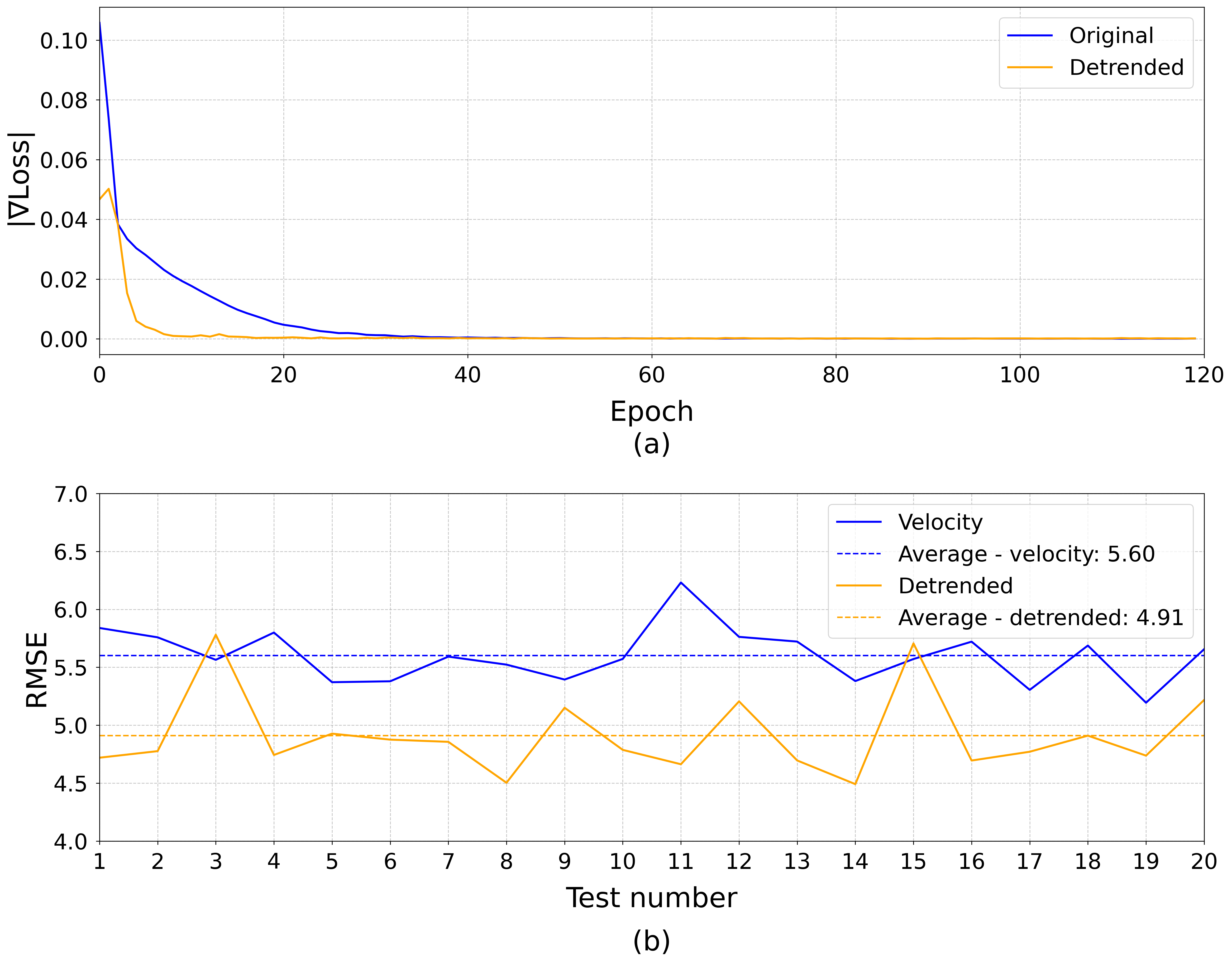
Using both the original and detrended data sets, we conduct 20 independent NN training runs for estimating reservoir changes due to CO 2 plume migration. Although both processes result in relatively low loss values (Figure 12a), the network trained on the detrended models converges significantly faster and yields the lowest final loss. This behavior reflects the advantage of restricting the velocity range by removing large-scale trends, which makes it easier for the network to capture the remaining (more localized) variations relevant for CO 2 migration. We also evaluate each run by computing the RMSE between the actual and predicted velocity models (Figure 12b). Evidently, networks trained on the detrended data consistently achieve lower RMSE values compared to those trained on the original data, so removing background trends can enhance network generalizability.
The detrended models also produce fewer errors and better capture the localized velocity variations due to CO 2 plume extension. The improved areas include shallow layers, reservoir horizons, and bedrock zones (Figure 13d). In future work, we will extend this approach to a representative range of velocity models to evaluate the benefits of detrending for seismic reservoir monitoring and imaging.

4.3. Double-Compression Test

We next evaluate the efficiency of the proposed double-compression framework by comparing it with a conventional training approach. To establish a baseline, we first generate “detrended” reservoir models as discussed above and simulate the corresponding seismic data. For the proposed method, we additionally employ HWT to reconstruct these models at multiple resolutions. We compared two training configurations. The first, representing a conventional approach, consisted of a single-stage training test. Using a two-encoder, two-decoder (2E2D) architecture, we trained the network on a redundantly decimated version of the original reservoir attribute dimensions ( 88 × 150 ). The second configuration evaluated the proposed double-compression framework using a multiresolution strategy. We first trained a network with two encoders and six decoders (2E6D) on progressively coarser reservoir models (from 2 × 2 , 4 × 4 , and 8 × 8 to 64 × 64 ). Upon convergence, we applied transfer learning to a secondary 2E2D network. During this stage, we froze the encoder weights and fine-tuned the decoder’s convolutional layers on higher-resolution targets ( 128 × 128 and 256 × 256 ).
Table 3 summarizes the run times and GPU memory usage for each training configuration, along with the corresponding percentage reductions relative to the baseline (Test 1). The first row (88 × 150) corresponds to the direct decimation approach (which serves as our reference) that has a 105-min run time and a 14 GB global GPU memory allocation. In contrast, the multiresolution method that starts from coarse grids (from 2 × 2 to 64 × 64) requires only 30 min and 10 GB of GPU memory, representing 71% and 33% reductions, respectively. Subsequently, we fine-tune at higher resolutions (128 × 128 and 256 × 256), which takes about 32 min with just 4 GB of GPU memory, corresponding to respective reductions of 70% and 73%. These results quantify the efficiency gains from training at multiple scales. The network learns coarser features at lower resolutions and then refines its predictions with minimal additional cost at higher resolutions. Freezing the encoder layers preserves essential feature representations, which allows the decoders to adapt to finer details with reduced computational overhead. This strategy should be particularly beneficial for large-scale geophysical models that are expensive to train from scratch at full resolution.
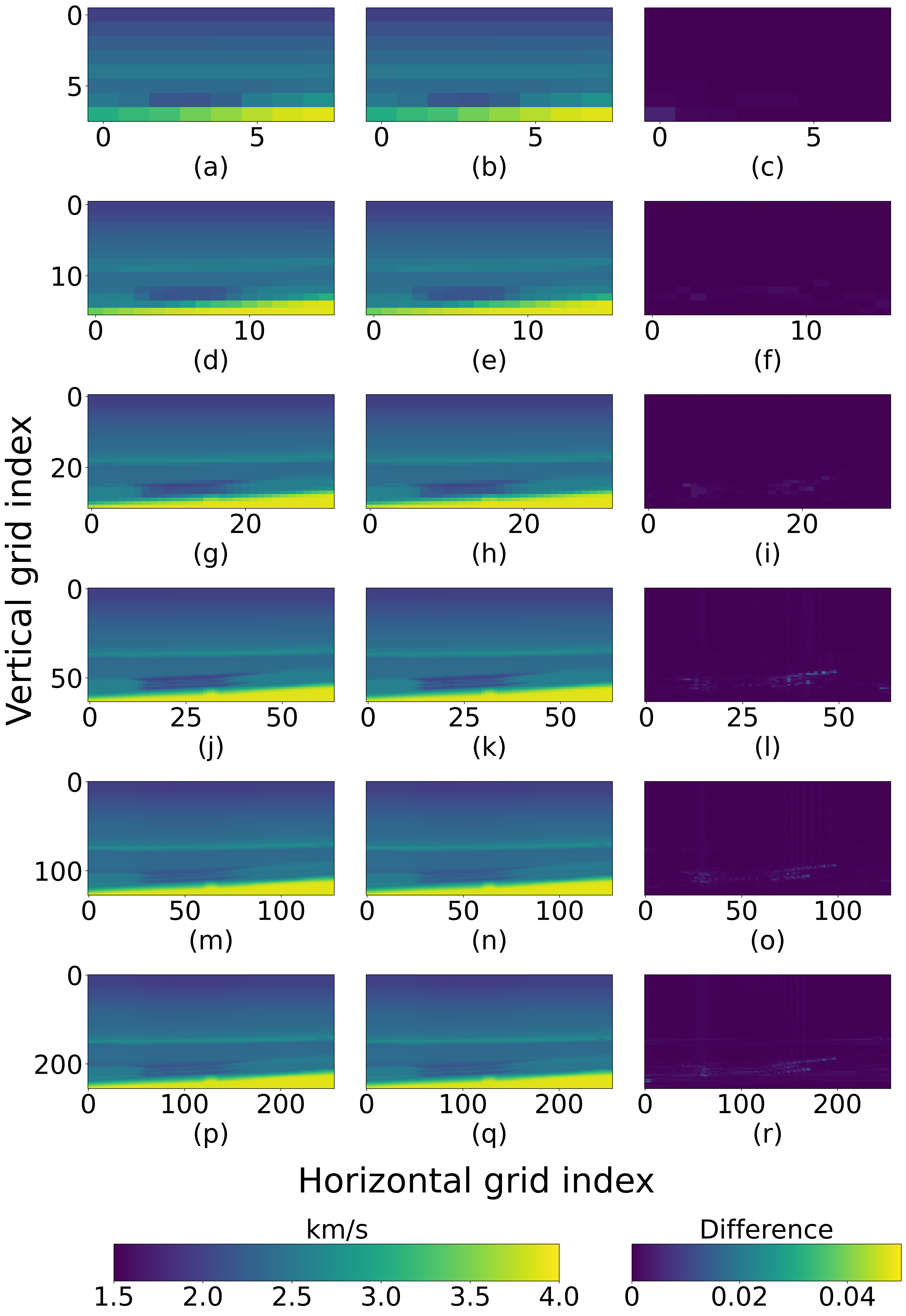
For multiresolution predictions of the elastic parameters ( V P , V S , ρ ), we employ a multi-NN strategy that leverages transfer learning to efficiently capture features at different scales. First, the initial network is trained for estimating the P-wave velocity using inputs that combine simulated seismic shots with four low-resolution V P representations of 8 × 8, 16 × 16, 32 × 32, and 64 × 64 (Figure 14). The low-resolution predictions capture the primary velocity trends with normalized errors below 0.04, which indicates that the network effectively learns the dominant coarse-scale features. Next, the pretrained network is fine-tuned to enhance predictions at higher resolutions of 128 × 128 and 256 × 256 . At this stage, the encoder layers are frozen to retain the low-resolution feature representations, while the decoder parts are updated to integrate finer details. As illustrated in Figure 14, the high-resolution predictions closely match the actual model with only minor artifacts.
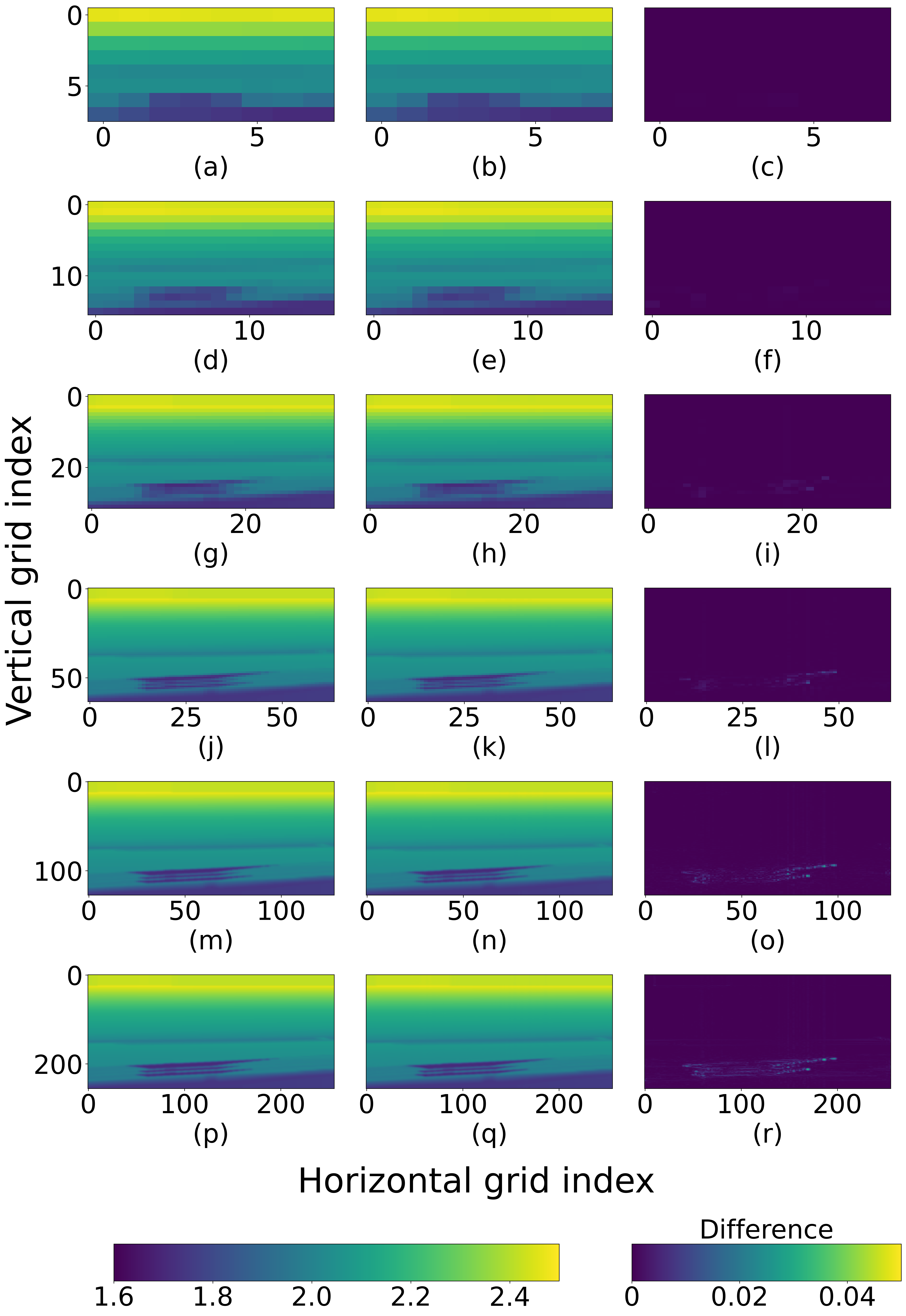
We apply a similar methodology to estimate the V P / V s ratio. Initially, the network is trained on low-resolution maps of V P / V s (Figure 15). The normalized differences are low (errors are less than 0.03), which indicates robust network’s performance even at coarser scales. The network trained on the low-frequency data is then used to fine-tune the model at higher resolutions by effectively transferring the learned features, which reduces computational cost.
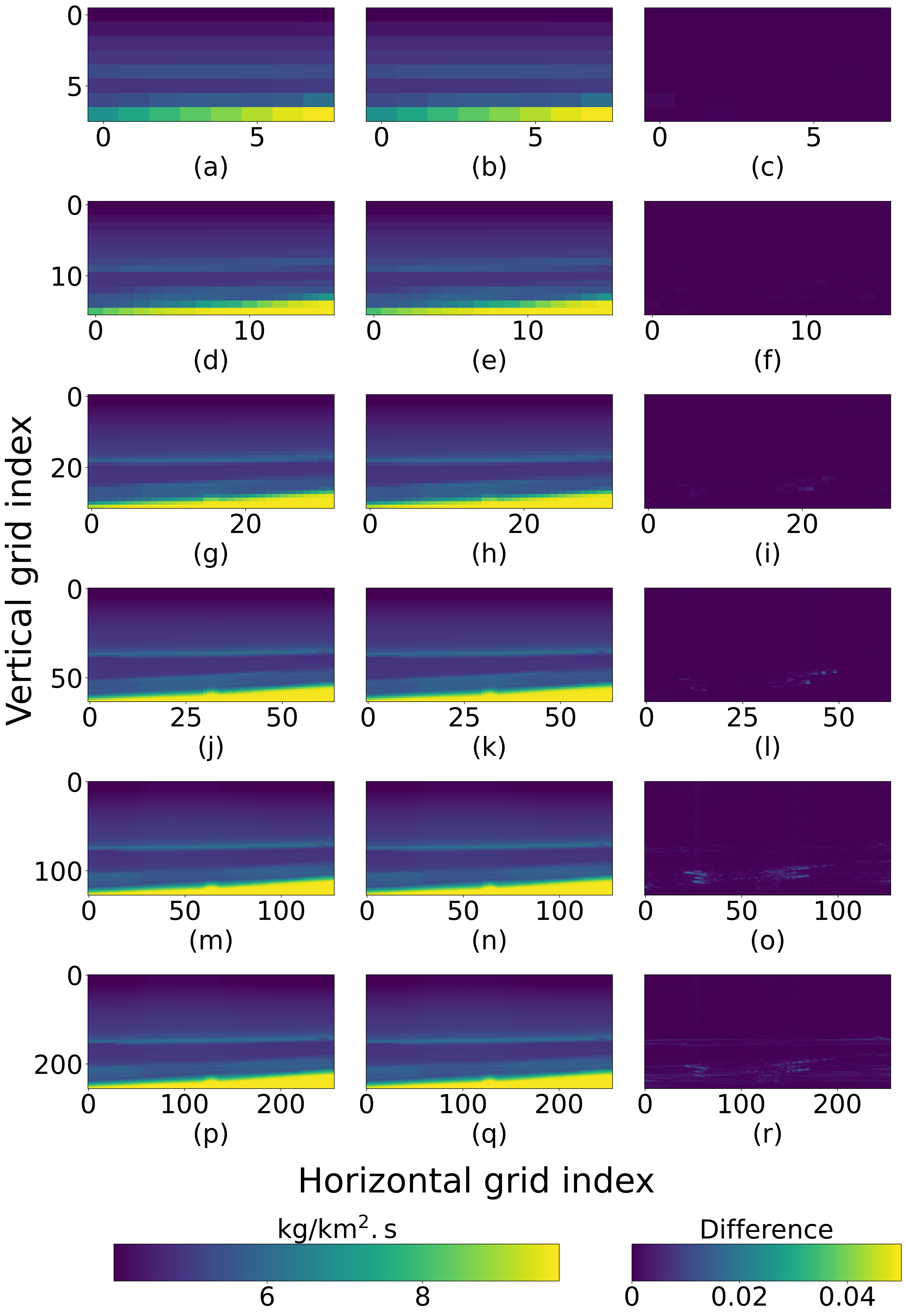
For acoustic impedance IP (later used to derive density), we follow the same two-stage training process with similar results (Figure 16).
In summary, the multiresolution, multi-NN strategy provides accurate elastic-parameter predictions across all six resolution levels at a fraction of the computational cost of the single-stage baseline. The broader implications of this efficiency are discussed below.

5. Discussion

The presented double-compression approach using several wavelet transforms and ML-driven latent representations addresses a major challenge in seismic reservoir monitoring-how to manage increasingly large data values while maintaining inversion accuracy. Our experiments confirm that compression based on the Haar wavelet transform (HWT) not only reduces storage demands but also feeds the neural network with sufficiently well sampled, lower-dimensional data. This preprocessing step significantly decreases run times and resource usage, which are essential for long-term, real-time monitoring applications.
The proposed wavelet-based compression preserves key geologic features (e.g., the parameter contrasts at model boundaries), which are crucial for elastic model building. The NN further compresses the data into a learned latent space tailored to the inverse problem at hand. This double-compression strategy leverages the strengths of both conventional (localized, scale-sensitive) transforms and data-driven (adaptable, predictive) models. Fine-tuning the network for such parameters as the V P / V S ratio and acoustic impedance benefits from having already learned the P-wave velocity distribution. Such transfer learning reduces training time and enhances model stability by mitigating the risks of overfitting.
Comparisons between different wavelet families reveal that the HWT consistently outperforms more complex transforms in preserving sharp boundaries, particularly in heterogeneous media (e.g., the BP model). At 1/16th of the original dimensions, decomposed coefficients still exhibit the main vertical and horizontal velocity changes and geologic structures. Moreover, using such a compressed velocity model, modeled wavefields have 0.08% energy loss, confirming that amplitude fidelity is essentially unaffected. Because compression is an extra stage in the workflow, we aim to use a wavelet basis function with minimal overhead. The Haar wavelet basis meets that requirement while maintaining a 16:1 reduction of the input model dimensions. The ability to achieve a high compression ratio while retaining critical information is essential for reservoir monitoring.
Three independent evaluations are discussed in this study. The model-side reconstruction RMSE (Figure 3 and Figure 4), the high-resolution residuals at the finest decomposition levels (Figure 8 and Figure 9), and the modeled wavefield energy loss (Table 2) all show the Haar wavelet producing the smallest distortion at high compression ratios for both the Kimberlina and BP models. These three consistent views also motivate the choice L = 4 for the low-level set assigned to CNN 1 and M = 6 for the high-level set assigned to CNN 2 in Algorithm 1 and Section 4.3. The level L = 4 is where the reconstruction RMSE and wavefield energy loss begin to differentiate the wavelet families, and M = 6 captures the highest-frequency detail still recoverable without a disproportionate computational overhead.
Another practical consideration involves parameter-space constraints. Bounding the velocity distribution through detrending helps accelerate network convergence. By subtracting large-scale background trends, the network can capture reservoir-specific perturbations more effectively. This finding is consistent with ML best practices, which include data normalization or parameter constraints to promote efficient training.
Numerical tests for the Kimberlina and BP models demonstrate that the artifacts caused by compression remain small and should not hamper amplitude analysis and seismic imaging. These results, obtained for 2D models, indicate that the proposed methodology should have an even larger impact on 3D applications, where computational and storage demands are much higher. Future work will incorporate adaptive wavelet transforms and more advanced NN architectures (e.g., attention-based models) to facilitate the capture of reservoir changes in more complex geological settings.
Beyond seismic reservoir monitoring, the double-compression approach can be extended to a wide range of geophysical inverse problems, including electromagnetic (EM) tomography, gravity/magnetic inversion, ground-penetrating radar, and full-waveform imaging. We can apply HWT to compress the wavefields during both forward and backward propagation. Additionally, we use multiresolution displacement components to calculate the residuals between the observed and modeled seismic data, which could improve convergence to the global minimum. However, demonstrating this requires additional research beyond the scope of the present discussion. In practice, this facilitates larger 3D domains or multi-physics couplings to operate on memory-limited GPU hardware and improves the feasibility of real-time seismic imaging and monitoring.
The present study has several limitations that point to natural directions of future work. The experiments are restricted to 2D isotropic media, while real subsurface settings often contain transverse isotropy with a tilted symmetry axis, fracture-induced anisotropy, and small-scale heterogeneity. Acquisition noise is not explicitly injected into the training set, which limits the assessment of robustness for realistic seismic acquisition geometry. The framework should be tested on field-acquired CCUS or hydrocarbon-monitoring data. The central scaling argument behind the framework—multi-resolution training to reduce GPU memory—is most valuable in 3D, so a follow-up study using the Sleipner 3D model is the immediate next step. Further extensions include refining the neural architectures (e.g., employing attention-based decoders) to further optimize performance across a wider range of geologic settings.

6. Conclusions

We introduced a double-compression framework for time-lapse seismic reservoir monitoring that combines Haar wavelet pre-compression of elastic parameter fields with a dual-encoder, multi-decoder CNN–LSTM and transfer learning across resolution scales (Algorithm 1, Figure 1, Figure 2, Figure 3, Figure 4 and Figure 5). The Haar wavelet hierarchy serves as a multi-resolution supervision curriculum for the network where levels { L 1 , , L 4 } are assigned to a low-resolution network ( CNN 1 ) and the remaining levels { L 5 , L 6 } are predicted by a higher-resolution network ( CNN 2 ) initialized from the pretrained CNN 1 weights, with only the multi-resolution decoder branches being fine-tuned (the encoders and the LSTM are kept frozen).
The general conclusion is that the synergy between deterministic, physics-meaningful wavelet pre-compression and learned, distribution-specific data compression yields measurable computational and accuracy gains. Compared with a redundant-decimation baseline that uses CNN on an 88 × 150 velocity field, the proposed framework reduces network training time by approximately 71% (from 105 to 30 + 32 min) and GPU memory usage by 33–73% (from 14 GB to 4–10 GB), while keeping the wavefield energy loss below 0.1% at a 16:1 model-dimension reduction (Table 2, M2 columns at 128 × 128 ). The normalized prediction errors of V P , V P / V S , and acoustic impedance are below 0.04 across all six resolution levels (Figure 14, Figure 15 and Figure 16). The multiresolution, multi-NN strategy reduces computational cost by limiting the number of parameters that require updating during fine-tuning while achieving sufficiently high prediction accuracy of the model parameters. The framework also circumvents the need to partition reservoir parameters into smaller patches to fit within GPU memory constraints (a practice that often leads to edge artifacts and requires costly retraining when local predictions fail) by predicting the entire reservoir parameter at the desired resolution.

Author Contributions

Conceptualization, A.M.A., J.S. and I.T.; methodology, A.M.A., J.S. and I.T.; investigation, A.M.A., J.S. and I.T.; visualization, A.M.A. and J.S.; writing—original draft preparation, A.M.A. and J.S.; writing—review and editing, A.M.A., J.S. and I.T.; supervision, I.T. All authors have read and agreed to the published version of the manuscript.

Funding

This research received no external funding.

Data Availability Statement

Data associated with this research are available and can be obtained by contacting the corresponding author.

Acknowledgments

This work was supported by the Consortium Project on Seismic Inverse Methods for Complex Structures at the Center for Wave Phenomena (CWP), Colorado School of Mines (CSM). We thank the A-Team and C-Team at CWP and Aaron Girard (CSM) for productive discussions and helpful suggestions.

Conflicts of Interest

The authors declare no conflicts of interest.

References

  1. Mizuno, T.; Calvez, J.L. Real-time passive seismic monitoring using DAS—Today’s solutions and remaining challenges. Lead. Edge 2024, 43, 24–32. [Google Scholar] [CrossRef]
  2. Yu, P.; Zhu, T.; Marone, C.; Elsworth, D.; Yu, M. DASEventNet: AI-Based Microseismic Detection on Distributed Acoustic Sensing Data From the Utah FORGE Well 16A (78)-32 Hydraulic Stimulation. J. Geophys. Res. Solid Earth 2024, 129, e2024JB029102. [Google Scholar] [CrossRef]
  3. Lumley, D.E. Long-term time-lapse seismic monitoring of CO2 injection and storage projects for 50–100 years of regulatory compliance. In Proceedings of the Sixth International Conference on Engineering Geophysics, Virtual, 25–28 October 2021; Society of Exploration Geophysicists: Houston, TX, USA, 2021; pp. 17–20. [Google Scholar]
  4. Martuganova, E.; Stiller, M.; Norden, B.; Henninges, J.; Krawczyk, C.M. 3D deep geothermal reservoir imaging with wireline distributed acoustic sensing in two boreholes. Solid Earth 2022, 13, 1291–1307. [Google Scholar] [CrossRef]
  5. Brown, L.; van der Baan, M. Time-lapse monitoring of saltwater disposal in Kansas and Oklahoma using ambient noise. In Proceedings of the Second International Meeting for Applied Geoscience & Energy, Houston, TX, USA, 28 August–1 September 2022; Society of Exploration Geophysicists: Houston, TX, USA, 2022; pp. 1551–1555. [Google Scholar]
  6. Queißer, M.; Singh, S.C. Full waveform inversion in the time lapse mode applied to CO2 storage at Sleipner. Geophys. Prospect. 2013, 61, 537–555. [Google Scholar] [CrossRef]
  7. Huang, C.; Zhu, T. Towards real-time monitoring: Data assimilated time-lapse full waveform inversion for seismic velocity and uncertainty estimation. Geophys. J. Int. 2020, 223, 811–824. [Google Scholar] [CrossRef]
  8. Liu, Y.; Tsvankin, I. Methodology of time-lapse elastic full-waveform inversion for VTI media. J. Seism. Explor. 2021, 30, 257–270. [Google Scholar]
  9. Huang, C.; Zhu, T.; Xing, G. Data-assimilated time-lapse visco-acoustic full-waveform inversion: Theory and application for injected CO2 plume monitoring. Geophysics 2023, 88, R105–R120. [Google Scholar] [CrossRef]
  10. Brankovic, M.; Gildin, E.; Gibson, R.L.; Everett, M.E. A Machine Learning-Based Seismic Data Compression and Interpretation Using a Novel Shifted-Matrix Decomposition Algorithm. Appl. Sci. 2021, 11, 4874. [Google Scholar] [CrossRef]
  11. Yang, Y.; Mandt, S.; Theis, L. An introduction to neural data compression. arXiv 2023, arXiv:2202.06533. [Google Scholar] [CrossRef]
  12. Elavarasi, K.; Vishnupriya, K. Enhancing the Computing Efficiency Through Data Compression for Machine Learning. In Proceedings of the Second International Conference on Data Science and Information System (ICDSIS), Hassan, India, 17–18 May 2024; IEEE: New York, NY, USA, 2024; pp. 1–6. [Google Scholar]
  13. Karami, A.; Yazdi, M.; Mercier, G. Compression of Hyperspectral Images Using Discerete Wavelet Transform and Tucker Decomposition. J. Sel. Top. Appl. Earth Obs. Remote Sens. 2012, 5, 444–450. [Google Scholar] [CrossRef]
  14. Tackie Ammah, P.N.; Owusu, E. Robust medical image compression based on wavelet transform and vector quantization. Inform. Med. Unlocked 2019, 15, 100183. [Google Scholar] [CrossRef]
  15. Parmar, H.M.; Scholar, P. Comparison of DCT and Wavelet based Image Compression Techniques. Int. J. Eng. Dev. Res. 2014, 2, 664–669. [Google Scholar]
  16. Grgic, S.; Kers, K.; Grgic, M. Image compression using wavelets. In Proceedings of the IEEE International Symposium on Industrial Electronics (Cat. No.99TH8465), Bled, Slovenia, 12–16 July 1999; IEEE: New York, NY, USA, 1999; pp. 99–104. [Google Scholar]
  17. Zhao, X.; Wang, L.; Zhang, Y.; Han, X.; Deveci, M.; Parmar, M. A review of convolutional neural networks in computer vision. Artif. Intell. Rev. 2024, 57, 99. [Google Scholar] [CrossRef]
  18. Aharon, M.; Elad, M.; Bruckstein, A. K-SVD: An algorithm for designing overcomplete dictionaries for sparse representation. IEEE Trans. Signal Process. 2006, 54, 4311–4322. [Google Scholar] [CrossRef]
  19. Mairal, J.; Bach, F.; Ponce, J.; Sapiro, G. Online dictionary learning for sparse coding. In Proceedings of the 26th Annual International Conference on Machine Learning, Montreal, QC, Canada, 14–18 June 2009; Association for Computing Machinery: New York, NY, USA, 2009; pp. 689–696. [Google Scholar]
  20. Schiavon, A.P.; Ribeiro, K.S.D.S.; Navarro, J.P.; Vieira, M.B.; Silva, P.M.C. 3D seismic data compression with multi-resolution autoencoders. In Proceedings of the SEG Technical Program Expanded Abstracts 2020, Virtual, 11–16 October 2020; Society of Exploration Geophysicists: Houston, TX, USA, 2020; pp. 1676–1680. [Google Scholar]
  21. Beckouche, S.; Ma, J. Simultaneous dictionary learning and denoising for seismic data. Geophysics 2014, 79, A27–A31. [Google Scholar] [CrossRef]
  22. Jia, Y.; Ma, J. What can machine learning do for seismic data processing? An interpolation application. Geophysics 2017, 82, V163–V177. [Google Scholar] [CrossRef]
  23. Fang, W.; Fu, L.; Liu, S.; Li, H. Dealiased seismic data interpolation using a deep-learning-based prediction-error filter. Geophysics 2021, 86, V317–V328. [Google Scholar] [CrossRef]
  24. Faouzi Zizi, M.O.; Turquais, P. A dictionary learning method for seismic data compression. Geophysics 2022, 87, V101–V116. [Google Scholar] [CrossRef]
  25. Jiang, F.; Tao, W.; Liu, S.; Ren, J.; Guo, X.; Zhao, D. An end-to-end compression framework based on convolutional neural networks. arXiv 2017, arXiv:1708.00838. [Google Scholar] [CrossRef]
  26. Toderici, G.; Vincent, D.; Johnston, N.; Hwang, S.J.; Minnen, D.; Shor, J.; Covell, M. Full Resolution Image Compression with Recurrent Neural Networks. In Proceedings of the Conference on Computer Vision and Pattern Recognition (CVPR), Honolulu, HI, USA, 21–26 July 2017; IEEE: New York, NY, USA, 2017; pp. 5435–5443. [Google Scholar]
  27. Liu, T.; Wang, J.; Liu, Q.; Alibhai, S.; Lu, T.; He, X. High-Ratio Lossy Compression: Exploring the Autoencoder to Compress Scientific Data. IEEE Trans. Big Data 2023, 9, 22–36. [Google Scholar] [CrossRef]
  28. Ma, S.; Zhang, X.; Jia, C.; Zhao, Z.; Wang, S.; Wang, S. Image and Video Compression with Neural Networks: A Review. Trans. Circuits Syst. Video Technol. 2020, 30, 1683–1698. [Google Scholar] [CrossRef]
  29. Theis, L.; Shi, W.; Cunningham, A.; Huszár, F. Lossy image compression with compressive autoencoders. arXiv 2017, arXiv:1703.00395. [Google Scholar] [CrossRef]
  30. Zhang, C.; He, X. Image Compression by Learning to Minimize the Total Error. Trans. Circuits Syst. Video Technol. 2013, 23, 565–576. [Google Scholar] [CrossRef]
  31. Schiavon, A.P.; Ribeiro, K.; Navarro, J.P.; Vieira, M.B.; Silva, P.M.C.E. 3-D Poststack Seismic Data Compression with a Deep Autoencoder. IEEE Geosci. Remote Sens. Lett. 2022, 19, 1–5. [Google Scholar] [CrossRef]
  32. Ahmed, M.A.; Tsvankin, I.; Liu, Y. High-Resolution Seismic Reservoir Monitoring with Multitask and Transfer Learning. EarthArXiv 2026. [Google Scholar] [CrossRef]
  33. Ahmed, N.; Natarajan, T.; Rao, K.R. Discrete Cosine Transform. IEEE Trans. Comput. 1974, C-23, 90–93. [Google Scholar] [CrossRef]
  34. Mallat, S. A Theory for Multiresolution Signal Decomposition: The Wavelet Representation. IEEE Trans. Pattern Anal. Mach. Intell. 1989, 11, 674–693. [Google Scholar] [CrossRef]
  35. Ning, J.; Wang, J.; Gao, W.; Liu, C. A Wavelet-Based Data Compression Technique for Smart Grid. Trans. Smart Grid 2011, 2, 212–218. [Google Scholar] [CrossRef]
  36. Alumbaugh, D.; Gasperikova, E.; Crandall, D.; Commer, M.; Feng, S.; Harbert, W.; Li, Y.; Lin, Y.; Samarasinghe, S. The Kimberlina synthetic multiphysics dataset for CO2 monitoring investigations. Geosci. Data J. 2024, 11, 216–234. [Google Scholar] [CrossRef]
  37. Shah, H. The 2007 BP anisotropic velocity-analysis benchmark. In Proceedings of the Expanded Abstracts of the 70th Annual International Conference and Exhibition of the European Association of Geoscientists and Engineers, London, UK, 11–14 June 2007; EAGE: Utrecht, The Netherlands, 2007; Available online: https://wiki.seg.org/wiki/2007_BP_Anisotropic_Velocity_Benchmark (accessed on 19 May 2026).
  38. Szu, H.; Telfer, B.; Garcia, J. Wavelet transforms and neural networks for compression and recognition. Neural Netw. 1996, 9, 695–708. [Google Scholar] [CrossRef]
  39. Paul, A.; Khan, T.Z.; Podder, P.; Ahmed, R.; Rahman, M.M.; Khan, M.H. Iris image compression using wavelets transform coding. In Proceedings of the 2nd International Conference on Signal Processing and Integrated Networks (SPIN), Noida, India, 19–20 February 2015; IEEE: New York, NY, USA, 2015; pp. 544–548. [Google Scholar]
  40. Myo Tun, H. Analysis on ECG data compression using wavelet transform technique. Int. J. Psychol. Brain Sci. 2017, 2, 127–140. [Google Scholar] [CrossRef]
  41. Taujuddin, N.S.A.; Lockman, N.A.B. Image compression using wavelet algorithm. In Proceedings of the International Seminar on the Application of Science & Mathematics 2011, Kuala Lumpur, Malaysia, 1–3 November 2011. [Google Scholar]
  42. Tschannen, M.; Agustsson, E.; Lucic, M. Deep generative models for distribution-preserving lossy compression. arXiv 2018, arXiv:1805.11057. [Google Scholar] [CrossRef]
  43. Wang, L.; Meng, D.; Wu, B.; Liu, N. Seismic inversion via closed-loop fully convolutional residual network and transfer learning. In Proceedings of the SEG International Exposition and Annual Meeting, Online, 11–16 October 2020; Society of Exploration Geophysicists: Houston, TX, USA, 2020; p. D031S057R002. [Google Scholar]
  44. Huang, Y.; Yang, H.; Zhang, J. Velocity model building via combining seismic slope tomography and supervised deep learning. Geophys. Prospect. 2025, 73, 67–79. [Google Scholar] [CrossRef]
  45. Alzahrani, H.; Shragge, J. Seismic velocity model building using neural networks: Training data design and learning generalization. Geophysics 2022, 87, R193–R211. [Google Scholar] [CrossRef]
  46. Simon, J.; Fabien-Ouellet, G.; Gloaguen, E.; Khurjekar, I. Hierarchical transfer learning for deep learning velocity model building. Geophysics 2023, 88, R79–R93. [Google Scholar] [CrossRef]
  47. Ngiam, J.; Khosla, A.; Kim, M.; Nam, J.; Lee, H.; Ng, A. Multimodal Deep Learning. In Proceedings of the International Conference on Machine Learning, Bellevue, WA, USA, 28 June–2 July 2011. [Google Scholar]
  48. Mosser, L.; Dubrule, O.; Blunt, M.J. Stochastic Seismic Waveform Inversion Using Generative Adversarial Networks as a Geological Prior. Math. Geosci. 2018, 52, 53–79. [Google Scholar] [CrossRef]
  49. Hochreiter, S.; Schmidhuber, J. Long Short-Term Memory. Neural Comput. 1997, 9, 1735–1780. [Google Scholar] [CrossRef]
  50. Kingma, D.P.; Ba, J. Adam: A method for stochastic optimization. arXiv 2017, arXiv:1412.6980. [Google Scholar] [CrossRef]
  51. Johnston, N.; Vincent, D.; Minnen, D.; Covell, M.; Singh, S.; Chinen, T.; Jin Hwang, S.; Shor, J.; Toderici, G. Improved Lossy Image Compression with Priming and Spatially Adaptive Bit Rates for Recurrent Networks. In Proceedings of the Conference on Computer Vision and Pattern Recognition; IEEE: New York, NY, USA, 2018; pp. 4385–4393. [Google Scholar]
  52. Pan, S.J.; Yang, Q. A Survey on Transfer Learning. IEEE Trans. Knowl. Data Eng. 2010, 22, 1345–1359. [Google Scholar] [CrossRef]
  53. Zhang, C.; Bengio, S.; Hardt, M.; Recht, B.; Vinyals, O. Understanding deep learning (still) requires rethinking generalization. Commun. ACM 2021, 64, 107–115. [Google Scholar] [CrossRef]
  54. Yosinski, J.; Clune, J.; Bengio, Y.; Lipson, H. How transferable are features in deep neural networks? In Proceedings of the 28th International Conference on Neural Information Processing Systems—Volume 2, Montreal, QC, Canada, 8–13 December 2014; MIT Press: Cambridge, MA, USA, 2014; pp. 3320–3328. [Google Scholar]
  55. Ruder, S. Neural Transfer Learning for Natural Language Processing. Ph.D. Thesis, National University of Ireland, Galway, Ireland, 2019. [Google Scholar]
  56. Araya-Polo, M.; Jennings, J.; Adler, A.; Dahlke, T. Deep-learning tomography. Lead. Edge 2018, 37, 58–66. [Google Scholar] [CrossRef]
  57. Wang, Z.; Bovik, A.; Sheikh, H.; Simoncelli, E. Image quality assessment: From error visibility to structural similarity. Trans. Image Process. 2004, 13, 600–612. [Google Scholar] [CrossRef]
  58. Jia, X.; Zwart, J.; Sadler, J.; Appling, A.; Oliver, S.; Markstrom, S.; Willard, J.; Xu, S.; Steinbach, M.; Read, J.; et al. Physics-Guided Recurrent Graph Networks for Predicting Flow and Temperature in River Networks. arXiv 2020, arXiv:2009.12575. [Google Scholar] [CrossRef]
  59. Gassmann, F. Über die Elastizität poröser Medien. Vierteljahr. Naturforsch. Ges. Zürich 1951, 96, 1–23. [Google Scholar]
  60. Mavko, G.; Mukerji, T. Seismic pore space compressibility and Gassmann’s relation. Geophysics 1995, 60, 1743–1749. [Google Scholar] [CrossRef]
  61. Liu, Y.; Feng, S.; Tsvankin, I.; Alumbaugh, D.; Lin, Y. Joint physics-based and data-driven time-lapse seismic inversion: Mitigating data scarcity. Geophysics 2023, 88, K1–K12. [Google Scholar] [CrossRef]
  62. Sigfusson, B.; Gislason, S.R.; Matter, J.M.; Stute, M.; Gunnlaugsson, E.; Gunnarsson, I.; Aradottir, E.S.; Sigurdardottir, H.; Mesfin, K.; Alfredsson, H.A.; et al. Solving the carbon-dioxide buoyancy challenge: The design and field testing of a dissolved CO2 injection system. Int. J. Greenh. Gas. Control 2015, 37, 213–219. [Google Scholar] [CrossRef]
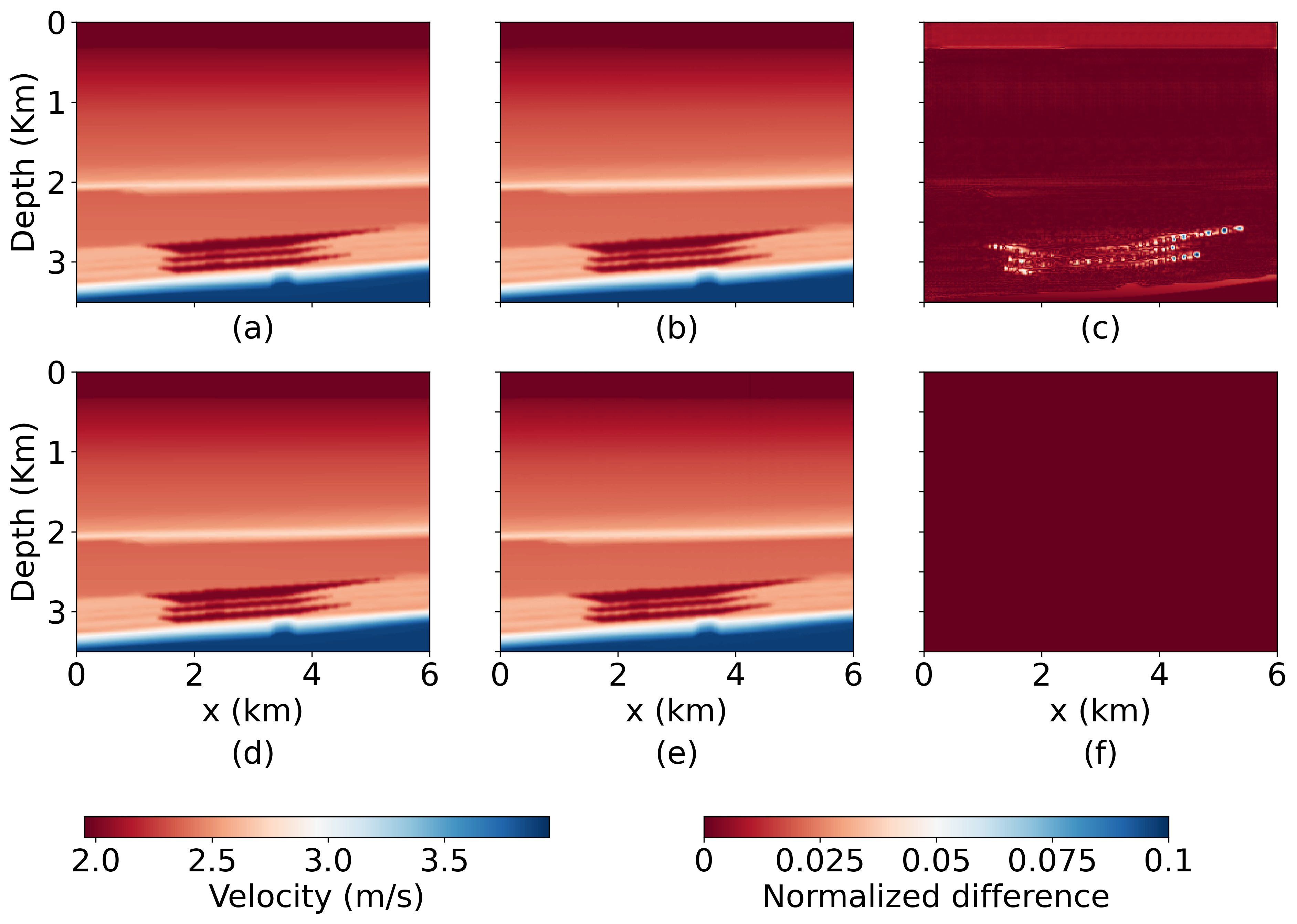
Figure 1. Reconstruction of the P-wave velocity field for the Kimberlina model using Haar wavelet transforms. (a) The original velocity model; (b) the model reconstructed using all coefficients; and (c) the difference between (a) and (b). The model reconstructed using (d) the base decomposition level; (e) two levels; (f) three levels; (g) four levels; (h) five levels; and (i) six levels.
Applsci 16 05352 g001
Figure 2. Reconstruction of the P-wave velocity field for the BP model using Haar wavelet transforms. (a) The original velocity model; (b) the model reconstructed using all coefficients; and (c) the difference between (a) and (b). The model reconstructed using (d) the base decomposition level; (e) two levels; (f) three levels; (g) four levels; (h) five levels; and (i) six levels.
Applsci 16 05352 g002
Figure 3. Reconstruction of the Kimberlina P-wave velocity model using three different wavelet transforms. The maximum decomposition levels are four [(ac)], and six [(df)]. (a,d) the Haar transform; (b,e) the Daubechies2 transform; and (c,f) the Biorthogonal transform.
Applsci 16 05352 g003
Figure 4. Reconstruction accuracy for the BP model using three different wavelets. (a,d) The Haar transform; (b,e) the Daubechies2 transform; and (c,f) the Biorthogonal transform where the maximum decomposition levels for the upper and lower rows are four and six, respectively.
Applsci 16 05352 g004
Figure 5. Flowchart of data compression using CNN encoders (left) and estimation of multiresolution outputs through multi-decoders (right).
Applsci 16 05352 g005
Figure 6. P-wave velocity fields (left column) and the corresponding detrended fields (right column) for the Kimberlina (a,b), BP (c,d), and Marmousi (e,f) models.
Applsci 16 05352 g006
Figure 7. Histograms of the P-wave velocity fields (top row) and their detrended versions (bottom row) for the Kimberlina (a,b), BP (c,d), and Marmousi (e,f) models.
Applsci 16 05352 g007
Figure 8. Difference between the original Kimberlina P-wave velocity model and the model reconstructed (a) using all decomposition levels; (b) six levels; and (c) five levels.
Applsci 16 05352 g008
Figure 9. Difference between the original BP P-wave velocity model and the model reconstructed (a) using all decomposition levels; (b) six levels; and (c) five levels.
Applsci 16 05352 g009
Figure 10. Vertical displacement computed for the Kimberlina model using (a) the original and reconstructed P-wave velocity models with dimensions of (b) 512 × 512; (c) 256 × 256; and (d) 128 × 128. The differences (e) between plots (a) and (b); (f) between plots (a) and (c); and (g) between plots (a) and (d).
Applsci 16 05352 g010
Figure 11. Vertical displacement computed for the BP model using (a) the original and reconstructed P-wave velocity models with dimensions of (b) 512 × 512; (c) 256 × 256; and (d) 128 × 128. The differences (e) between plots (a) and (b); (f) between plots (a) and (c); and (g) between plots (a) and (d).
Applsci 16 05352 g011
Figure 12. (a) Gradient of the mean training losses from 20 repeated experiments for the original (blue) and detrended (orange) Kimberlina P-wave velocity models. (b) The root-mean-square-error (RMSE) for the 20 experiments for the original (blue) and detrended (orange) P-wave velocity models.
Applsci 16 05352 g012
Figure 13. P-wave velocity field for the Kimberlina model. (a) The actual model; (b) the predicted model; and (c) the normalized difference between (a) and (b). (d) The detrended model; (e) the prediction based on the detrended model; and (f) the difference between (d) and (e).
Applsci 16 05352 g013
Figure 14. Multiresolution predictions of the Kimberlina P-wave velocity field. The left column shows the actual field, the middle column the predicted field, and the right column the normalized error of the prediction. Dimensions (resolution): (ac) 8 × 8; (df) 16 × 16; (gi) 32 × 32; (jl) 64 × 64; (mo) 128 × 128; and (pr) 256 × 256.
Applsci 16 05352 g014
Figure 15. Multiresolution predictions of the V P / V s ratio for the Kimberlina model. The left column shows the actual model, the middle column the predicted model, and the right column the normalized error of the prediction. Dimensions (resolution): (ac) 8 × 8; (df) 16 × 16; (gi) 32 × 32; (jl) 64 × 64; (mo) 128 × 128; and (pr) 256 × 256.
Applsci 16 05352 g015
Figure 16. Multiresolution predictions of the acoustic impedance for the Kimberlina model. The left column shows the actual model, the middle column the predicted model, and the right column the normalized error of the prediction. Dimensions (resolution): (ac) 8 × 8; (df) 16 × 16; (gi) 32 × 32; (jl) 64 × 64; (mo) 128 × 128; and (pr) 256 × 256.
Applsci 16 05352 g016
Table 1. Compression sizes and percentage reductions for the 2D Kimberlina P-wave velocity model at various wavelet decomposition levels. The first row lists the original model dimensions, while the second row depicts a redundantly subsampled version of the model (downsampled by factors of three vertically and four horizontally). Rows three to eight correspond to HWT reconstructions using different decomposition levels.
Model DimensionsSize (MB)Percentage Reduction (%)
[ 350 × 600 ] 420
[ 88 × 150 ] 5.398.7
Level 01– [ 8 × 8 ] 0.0599.9
Level 02– [ 16 × 16 ] 0.299.9
Level 03– [ 32 × 32 ] 0.899.8
Level 04– [ 64 × 64 ] 3.399.2
Level 05– [ 128 × 128 ] 13.196.8
Level 06– [ 256 × 256 ] 54.487.0
Table 2. Energy loss (in percent) for the BP and Kimberlina (Kim) models, shown for each wavelet transform and output size, and for the displacement components u x , u z , and u = u x 2 + u z 2 .
ComponentOutputHaarDb2Sym2Bior1.3Coif2
BP Kim BP Kim BP Kim BP Kim BP Kim
512 × 5120.0%0.0%0.0%0.0%0.0%0.0%0.0%0.0%0.0%0.0%
u256 × 2560.0%0.0%0.1%0.04%0.1%0.04%2.2%0.04%24.5%0.26%
128 × 1280.0%0.01%1.3%0.21%1.3%0.21%11.6%0.44%106.1%0.99%
512 × 5120.0%0.0%0.0%0.0%0.0%0.0%0.0%0.0%0.0%0.0%
u z 256 × 2560.1%0.1%4.0%0.6%4.0%0.6%3.0%0.5%14.3%2.6%
128 × 1280.1%0.1%13.2%1.2%13.2%1.20%9.8%7.8%77.7%7.7%
512 × 5120.0%0.0%0.0%0.0%0.0%0.0%0.0%0.0%0.0%0.0%
u x 256 × 2560.2%0.0%8.8%0.02%8.8%0.02%7.0%0.03%22.8%0.23%
128 × 1280.2%0.0%18.8%0.22%18.8%0.22%17.0%0.18%159.3%0.95%
Table 3. Comparison of CNN architectures based on run time and GPU usage. Test 1 uses a redundantly decimated model with a 2E2D architecture. Test 2 first trains a 2E6D network at multiple coarser resolutions and then fine-tunes a 2E2D network for higher resolutions.
ArchitectureModel
Dimension
Run Time
(min)
Run Time
Reduction (%)
Memory
(GB)
Memory
Reduction (%)
2 E & 2 D (Test 1)88 × 15010514
2 E & 6 D (Test 2)2 × 2
4 × 4
8 × 8
16 × 16
32 × 32
64 × 64
30711033
2 E & 2 D (Test 2)128 × 128
256 × 256
3270473
Disclaimer/Publisher’s Note: The statements, opinions and data contained in all publications are solely those of the individual author(s) and contributor(s) and not of MDPI and/or the editor(s). MDPI and/or the editor(s) disclaim responsibility for any injury to people or property resulting from any ideas, methods, instructions or products referred to in the content.