Simulation Model for Electrical Operation in Agrivoltaic Power Plants: Nine Hourly Panel Orientation Modes

Abstract

In an agrivoltaic plot, the hourly panel tracking angle governs electricity, on-site economics, avoided carbon dioxide, irrigation demand and crop yield. Operating for photovoltaic output alone discards that space, and does so when a midday kilowatt-hour has lost its value: 715 h of the studied season carried a non-positive export price, 517 of them at midday. This work formalizes the electrical operating layer of a mechanistic hourly simulator as nine panel-orientation modes, each a constrained program solved deterministically by sequential quadratic programming, a dense angular scan, or both. Two modes keep an energy-proportional objective non-degenerate through an adaptive clean-grid switch and an economics–carbon weighting anchored on the crop. The catalog is a framework, demonstrated over a 153-day season on a 66 kWp single-axis sage (Salvia officinalis) plot near Valencia, Spain. Seasonal photovoltaic energy ranged from 57.0 to 31.9 MWh, plot-mean relative yield from 95% to 109%, and worst-plant protection from 61% to 94%. Energy maximization sits at a flat extreme of the frontier: the Pareto mode gained 11.4 yield points and 31 worst-plant points for 1.1% less energy. Avoided carbon dioxide varied by 2.1% across the nine modes, so a carbon objective is degenerate with energy without an interior term.

1. Introduction

The increasing pressure on agricultural land from two competing demands—food production and renewable energy generation—has emerged as one of the central resource allocation challenges of the century [1]. Arable surface is finite, and the rapid expansion of ground-mounted photovoltaic installations required to meet decarbonization targets places it in direct competition with the cropland needed to sustain growing populations [2]. A structural response to this tension is offered by agrivoltaic (APV) systems, dual-use installations in which solar panels are elevated above crops so that a single plot produces both electricity and agricultural produce. Since the foundational work of Goetzberger and Zastrow [3] and the field trials of Dupraz et al. [4], the discipline has expanded to encompass fixed-tilt structures, single- and dual-axis trackers, vertical bifacial configurations, and dynamic systems in which panel inclination adapts continuously to operational objectives. Field campaigns on dynamic trackers have reported improved crop water-use efficiency and air- and soil-temperature reductions of a few degrees for a range of shade-tolerant aromatic species [5,6]. Dynamic panel tracking adds a degree of freedom that enables hour-by-hour trade-offs between electricity production and crop radiation receipt, a capacity that fixed-tilt systems cannot replicate.

Alongside this diversification in hardware, the objectives governing system optimization have multiplied. Energy maximization, agronomic protection, economic benefit, self-consumption maximization and carbon-emission reduction each constitute recognized optimization targets. Yet, existing tools seldom integrate more than two of these simultaneously and rarely compare them under identical boundary conditions.

• Energy-centric platforms such as PVsyst, HOMER, PVGIS, and SAM [7,8] resolve the electrical side in detail but treat the crop, when at all, as a fixed loss.
• Crop-centric frameworks such as STICS, DSSAT, and the agrivoltaic adaptation of AquaCrop integrated by Bellone et al. [9] resolve the agronomy but do not optimize the panel orientation against economic or carbon signals.

The review of Zainali et al. [10] finds that most published models assemble stand-alone tools ex post, a conclusion shared by the syntheses of Coluccia et al. [11], Campana et al. [12] and Renno and Di Marino [13]. Crop-aware tracking control has been treated by Bruno et al. [14], Tekie et al. [15], Amadeh et al. [16] and Stuhlmacher et al. [17], and the operation of an APV plot against market signals by Mohseni and Brent [18,19]. In both groups the data exchange is unidirectional and there is no within-step feedback, so the optimizer cannot react to crop stress and the crop model cannot react to the panel-induced microclimate, and no alternative operating objectives are compared under identical boundary conditions. The site-specific optima of Berrian et al. [20] and Mazzeo et al. [21] confirm that these couplings matter and appear only at hourly resolution. Our own comparison of fixed-tilt and single-axis strategies [22] showed that the ranking of two orientation strategies can invert between an energy criterion and an economic criterion, which motivates the present paper.

A second reason the operating objective matters is that the value of a generated kilowatt-hour has become strongly time-dependent. Between 2021 and 2025 the Spanish day-ahead market moved from comparatively flat, uniformly positive prices to a structure with hundreds of hours at or below zero concentrated in the central solar hours, so that a midday kWh is now worth a fraction of a dawn or dusk one. The grid carbon intensity moves the same way, cleanest at midday, which is why an hourly series is used here rather than an annual average. The distinction between time-varying and average emission factors, and its consequences for the assessment of a distributed generator, is treated by Siler-Evans et al. [23], Tranberg et al. [24] and Goldsworthy and Aryai [25], when solar and wind dominate, so midday photovoltaic (PV) displaces near-zero-carbon electricity and avoids little $\mathrm{C}{\mathrm{O}}_2$. Price and carbon value therefore collapse together at the same hours in which an energy-maximizing plant generates most of its electricity, and operating an agricultural PV asset for generation volume becomes the wrong objective. This result is invisible to a static levelized cost versus tariff comparison and only surfaces once the hourly market and carbon series enter the simulation as inputs and propagate through every time step.

The simulator that underlies this study (a mechanistic, hourly, spatially resolved APV model) closes the coupling gap by placing the orientation optimizer inside the hourly loop and ahead of the radiation and microclimate sub-models. It resolves the panel geometry, the radiation that reaches each plant, the canopy microclimate and the crop response at hourly resolution. The simulator is deliberately energy-centric. The decision variable is always the panel orientation, so the crop is never the quantity being scheduled. Its agronomic sub-model is nonetheless mechanistic and fully resolved, per plant and per hour, rather than a reduced-form generator of constraints: it supplies the yield ratio that bounds the energy optimization in the modes where the crop is a limiting factor, and the criterion that the orientation answers to in the two modes where the crop is the objective. The crop parameters used here are drawn from the published results of a dynamic-tracker field trial on six aromatic species [5,6]. The present paper extends the optimizer from the four energy-yield modes to the full multi-objective decision space. It formalizes nine operating modes spanning energy, on-site economics, avoided ${\mathrm{CO}}_2$, irrigation-water (pumping energy) demand and crop yield, and characterizes their trade-offs on a sage (Salvia officinalis) plot near Valencia (Spain), over a full growing season, driven by 2025 Spanish hourly market and grid-carbon series, and it maps the resulting energy, yield, economic, carbon and water trade-off surface. What that mapping quantifies is a migration of value away from the generated kilowatt-hour and toward the agrivoltaic co-product, together with its demand-side and carbon consequences.

The research question is whether the panel-orientation decision of an APV plot can be posed and solved, at hourly resolution, as a genuine multi-objective program across the energy-water-food nexus, and whether the nine modes yield distinct, non-degenerate operating points.

The hypothesis is that the objectives with an interior optimum in the tracking angle (economic benefit, including a crop co-product, crop yield and crop water) compete with the single-peaked energy objective strongly enough to produce a non-trivial Pareto geometry, whereas objectives collinear with energy in the angle (avoided ${\mathrm{CO}}_2$ per kWh, energy revenue per kWh) do not, and require an interior term to become non-degenerate. The crop chosen for the demonstration is sage (Salvia officinalis), a Mediterranean aromatic whose moderate shade response makes the yield objective an active rather than saturated competitor. The crop is nevertheless a constraint and a co-product here, not the quantity being scheduled. All nine modes arbitrate the same physical decision, and they differ in the signal they answer to: hourly market price, grid carbon intensity, demand set-point, the pumping energy the plot itself consumes, or the crop response to the plot. The agronomic model enters to verify that the crop requirement or objective is met at every hour, and to price the co-product.

The claim evaluated here is delimited accordingly. This paper assesses the operating layer itself: the distinctness and the internal consistency of the nine modes, and the structure of the trade-off surfaces that they trace. The crop parameters are literature-based and were not fitted to the case study.

Section 2 formalizes the nine modes and the common solver. Section 3 gives the configuration of the demonstration plot. Section 4 reports the season-long results. Section 5 discusses the trade-off geometry and its operational consequences. Section 6 concludes.

2. Materials and Methods

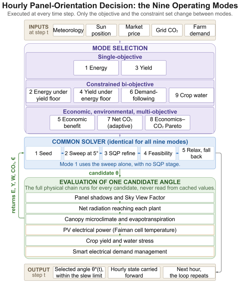
Figure 1 shows the decision that this paper formalizes. The orientation optimizer runs inside the hourly loop, and ahead of the radiation and microclimate sub-models. A candidate orientation is therefore evaluated by execution of the full geometric and biophysical chain that the orientation would produce, and not from cached values. This is what makes the nine modes solvable at hourly resolution over a multi-month horizon.

The optimizer sits above a physical evaluator. For a candidate orientation, the evaluator returns the array electrical energy, the radiation intercepted by each plant, the canopy microclimate, the evapotranspiration and the resulting relative yield. It assembles standard formulations: the solar position follows the NREL Solar Position Algorithm [26], the cell temperature follows the Faiman model [27] with the coefficients given in Section 3.1, the electrical power follows the usual derating form, the evapotranspiration follows FAO-56 Penman–Monteith [28], and the shading of each plant is resolved through an analytical per-pixel sky view factor. This section formalizes the nine operating modes and the common solver.

2.1. The Common Decision Problem

Every mode selects the hourly tracking angle by maximizing a mode-specific objective subject to a mode-specific constraint set and the tracker’s mechanical limits. The objective and the constraint set are what define each mode. Two structural properties are exploited throughout.

• First, the energy objective is single-peaked in the tracking angle, with its maximum at the solar-tracking orientation, so any objective proportional to it inherits the same optimizer and cannot, on its own, produce an interior trade-off.
• Second, the crop-related objectives (yield, water and the crop co-product term of the economic benefit) have an interior optimum in the tracking angle, because moderate shade can raise a shade-tolerant crop’s performance while extreme shade harms it. It is this interior optimum, in conflict with the energy peak, that generates a non-degenerate trade-off.

The yield and water metrics can be evaluated on four bases (accumulated-global, current-global, accumulated-individual, current-individual), and the two roles of the yield metric are described below:

• Where it acts as a constraint (a floor, in Modes 2 and 9), the metric is evaluated on the accumulated-individual basis, which protects the worst-performing plant and delivers the agronomic guarantee.
• Where it acts as an objective to be maximized (in Modes 3 and 4), the metric is evaluated on the same accumulated-individual basis, so that the objective, the floor and the reported indicator are stated in the same terms.

The accumulated-individual basis is used in both roles because the yield is reported at the season scale and per plant, so the objective of Modes 3 and 4, the floor of Modes 2 and 9 and the indicators of Section 2.6 all refer to one quantity. The ratio refers the accumulated yield of each plant to the accumulated yield of its baseline twin over the same hours, so both terms grow together and the ratio keeps responding to the orientation of the step. The current-global alternative that the implementation also admits is more sensitive to the angle of the step, but it is a plot mean and therefore does not protect the individual plant, which is the quantity that a yield mandate acts on.

The same movement rule applies to all nine modes: the array is driven to the optimum of each step within its mechanical range, with the optional movement dead-band of the implementation set to zero for the Section 3 simulations.

2.2. Overview of the Nine Operating Modes

Table 1. The nine hourly panel-orientation modes, the objective each optimizes, the constraint or rule that defines it, and its typical operating context. The formal description of each mode is given in Section 2.3, Section 2.4 and Section 2.5.

#	Mode	Objective	Constraint/Rule	Typical Use
1	Electrical energy	Maximize array electrical energy	None	PV-priority plots
2	Electrical energy under yield floor	Maximize energy	Per-plant relative yield floor	Plots under an APV yield mandate
3	Yield	Maximize relative crop yield	Electrical energy tie-break at equal yield	Pure agronomic impact studies
4	Yield under electrical energy floor	Maximize relative yield	Minimum electrical energy floor	Grid-tied self-consumption with a hard load guarantee
5	Economic benefit	Maximize on-site benefit	None	Market participation
6	Demand-following	Match generation to a demand target	Two-sided energy set-point	Islanded or export-constrained demand-matching
7	Net $\mathrm{C}{\mathrm{O}}_2$ (adaptive)	Dirty grid: maximize energy Clean grid: maximize yield	Self-sufficient on clean-grid hours Switch on grid carbon intensity	Carbon-signal following operation
8	Economics–$\mathrm{C}{\mathrm{O}}_2$ Pareto	Maximize a weighted sum of economic benefit and avoided $\mathrm{C}{\mathrm{O}}_2$	Weight sweeps the front	Market + Carbon co-optimization
9	Crop-water minimization	Minimize pumping energy and water consumption	Per-plant relative yield floor (active in this study)	Water-scarce sites

summarizes the nine modes, including the objective each optimizes, the constraint or rule that defines it and the operating context it targets. The subsections that follow give the formal objective and the rationale for each. They are grouped by mathematical structure: single-objective (Section 2.3), constrained bi-objective (Section 2.4), and economic, environmental and multi-objective (Section 2.5).

2.3. Single-Objective Modes

2.3.1. Mode 1: Pure Electrical Energy Maximization

The objective is the array electrical energy, including the cell-temperature derating of the conversion efficiency, with no agronomic constraint:

$$\max E\left(x\right) \mathrm{s}.\mathrm{t}. x_{\min } \le x \le { x}_{\max }$$

(1)

The procedure is hybrid rather than purely gradient-based. An analytical ideal-orientation seed is refined by a dense one-dimension sweep evaluated with the full array model, including mutual inter-row shading, and the better result is kept. For the single-axis configuration of the demonstration plot, the closed-form tracker orientation is already the maximizer of the swept objective at every step, so Mode 1 is a close energetic upper bound rather than a guaranteed one. Section 5.1 reports the size of that margin.

2.3.2. Mode 3: Pure Yield Maximization with Electrical Energy Tie-Break

The objective is the relative crop yield, with a lexicographic tie-break that, at equal yield, prefers the orientation of greater electrical generation:

$$\max {\displaystyle \frac{Y_{\mathrm{A}\mathrm{P}\mathrm{V}}\left(x\right)}{Y_{\mathrm{r}\mathrm{e}\mathrm{f}}}}+\epsilon E_{\mathrm{n}\mathrm{o}\mathrm{r}\mathrm{m}}\left(x\right) \mathrm{s}.\mathrm{t}. {\mathrm{x}}_{\min } \le \mathrm{x} \le { \mathrm{x}}_{\max }$$

(2)

The weight on the energy term is small enough that it never overrides the yield term, and its role is to resolve the low-elevation degeneracy in which several orientations give the same agronomic outcome, without an unnecessary energy penalty. The yield is evaluated on the accumulated-individual basis, so the objective remains responsive to the angle throughout the season.

2.4. Constrained Bi-Objective Modes

2.4.1. Mode 2: Electrical Energy Under a Crop-Yield Floor

Energy is maximized subject to a minimum relative yield constraint:

$$\max E\left(x\right) \mathrm{s}.\mathrm{t}. {\displaystyle \frac{Y_{\mathrm{APV}}\left(x\right)}{Y_{\mathrm{ref}}}} \ge {\eta }_{\mathrm{yield}} ; x_{\min } \le x \le x_{\max }$$

(3)

The DIN SPEC 91434 standard [29] sets a regulatory minimum relative yield of 66%. This study applies a stricter, self-imposed floor of 80%, which therefore exceeds the DIN minimum by a wide margin. The floor is imposed on the accumulated individual yield, protecting the plant in the worst situation.

Because the constraint applies to the season-accumulated yield, it is enforced along a rising seasonal trajectory rather than only at harvest, with the required floor ramped up over the campaign so that early over-shading cannot leave the target unreachable after a low-radiation day. When the constraint is infeasible for the worst plant, it is relaxed from the minimum to the mean individual ratio before any objective fallback, so the array moves as far as possible to benefit the ensemble instead of stalling on a single unrecoverable plant.

2.4.2. Mode 4: Yield Under an Electrical Energy Floor

This mode is the dual of Mode 2. The yield, evaluated on the accumulated-individual basis and with the energy tie-break of Mode 3, is maximized subject to a minimum energy constraint that covers the farm’s critical loads, such as the irrigation pump, refrigeration and lighting:

$$\max \left[{\displaystyle \frac{Y_{\mathrm{APV}}\left(x\right)}{Y_{\mathrm{ref}}}} + \mathsf{\epsilon }{E}_{\mathrm{norm}}\left(x\right)\right] \mathrm{s}.\mathrm{t}. E\left(x\right) \ge E_{\min }; x_{\min } \le x \le x_{\max }$$

(4)

The floor covers the critical loads of the farm. It can be applied as an input or as a scheduled constraint within a time window. In this study, it is applied in its scheduled form: within the window from 10:00 to 17:00 local time, the array must cover the pumping load of the step plus a fixed surplus of 30 kWh, and outside that window the floor is not enforced. If the energy floor is infeasible, a configurable fallback policy resolves the step by energy priority (revert to Mode 1) or crop priority (revert to Mode 3). Because the floor is one-sided, unlike Mode 6, generation above the minimum is permitted rather than penalized.

2.4.3. Mode 6: Electrical Demand-Following with Agronomic Maximization

This mode tracks a target energy demand rather than maximizing generation. The maximum attainable energy at the sun-pointing angle is computed first. If it does not reach the target, the demand cannot be met, and the mode reverts to maximum tracking, which is Mode 1. If it exceeds the target, some orientation matches the demand exactly. The problem is then solved in two phases. The generation is first driven as close as possible to the demand set-point. Among the orientations that achieve that closest match, the one that maximizes the relative crop yield is then selected. The surplus generation capacity above the set-point becomes an agronomic degree of freedom.

Unlike the one-sided floor of Mode 4, this two-sided set-point curtails the surplus above demand. Because the energy curve is single-peaked in the tracking angle, the demand is in general matched by two orientations, one on each side of the tracking peak. The second phase retains the orientation that casts the least shade on the canopy.

The demand target is the sum of the irrigation-pump load and a background baseload. The pump load alone is negligible against the array output, so a background load is added to make the target meaningful. For the simulations in this paper, it is dependent on the time of day: 22 kW within the window from 10:00 to 17:00 and 5 kW for the rest of the day. This load represents the on-farm processing of the harvested aromatic biomass, for which steam distillation and cold storage are the usual energy-intensive operations. The daytime value is one-third of the rated array capacity, so the set-point binds through the central hours and does not bind at the margins of the day.

2.4.4. Mode 9: Crop Water (Pumping Energy) Minimization

This mode is a pure demand-side lever. The crop water consumed is supplied by irrigation, whose pumped volume is proportional to the crop water through the application efficiency, and whose pumping energy is proportional to that volume through the manometric head and pump efficiency. Minimizing crop evapotranspiration is therefore, up to a constant, minimizing the pump’s electrical demand. The objective minimizes crop water demand under an active minimum-yield constraint:

$$\min W\left(x\right) \mathrm{s}.\mathrm{t}. {\displaystyle \frac{Y_{\mathrm{APV}}\left(x\right)}{Y_{\mathrm{ref}}}} \ge {\eta }_{\mathrm{yield}} ; x_{\min } \le x \le { x}_{\max }$$

(5)

The panel reduces only the radiative term of the FAO-56 Penman–Monteith evapotranspiration through shading (lower net radiation $R_{\mathrm{n}}$). The aerodynamic term is driven by macroclimatic wind and vapor-pressure deficit and does not respond to the tilt. There is consequently an irreducible evapotranspiration floor, and this mode reduces crop water down to that floor, not below it, which acts as a physical limit that bounds what the demand-side lever can deliver.

The yield floor is active in this mode. Therefore, Mode 9 is not an unconstrained water optimum, but the least-water orientation that still satisfies the agronomic guarantee.

2.5. Economic, Environmental and Multi-Objective Modes

2.5.1. Mode 5: Total Economic Benefit

The objective is the total hourly economic benefit, combining the energy revenue streams with the crop co-product value:

$$\max [B_{\mathrm{self}} + B_{\mathrm{comm}}+ B_{\mathrm{grid}} - C_{\mathrm{deficit}} + B_{\mathrm{crop}}] \left(x\right) \mathrm{s}.\mathrm{t}. x_{\min } \le x \le x_{\max }$$

(6)

The energy value follows a self-consumption, to community, to grid deficit priority, with curtailment at negative prices. The community tier is not populated in this single-plot demonstration, so the cascade reduces to self-consumption and grid exchange.

The crop term values the fresh growth of the step at a fixed reference dry-matter fraction, and not at the transient value of the step. The incentive therefore rests on the actual dry growth, which is the intercepted radiation multiplied by the radiation-use efficiency. The objective then has an interior optimum in the angle, instead of moving to the tilt that maximizes the transient water content during negative-price hours. Without this choice, the economic objective would inherit the single peak of the energy objective and would collapse onto Mode 1 whenever prices are positive.

The step objective and the reported indicator are therefore two different quantities. The step objective values the crop co-product through a stable reference proxy, because an online decision cannot use a harvest that has not yet occurred; the reported balance of Section 4 values the harvest as it would be sold. Mode 5 is consequently not guaranteed to rank first on the reported balance, and Section 5.3 states the crop prices at which the ranking changes.

2.5.2. Mode 7: Net CO₂ Minimization with an Adaptive Clean/Dirty Grid Switch

Every kilowatt-hour the array generates displaces one from the grid and avoids its carbon content, so the avoided carbon dioxide is proportional to the generation and an objective that minimizes it through the orientation alone reproduces Mode 1 exactly, without new behavior. Mode 7 therefore does not add a carbon term to the energy objective. It selects which objective applies at each hour, by comparing the grid carbon intensity of that hour against a threshold, which gives two branches:

$$\max E\left(x\right) \mathrm{s}.\mathrm{t}. x_{\min } \le x \le x_{\max } \left(\mathrm{dirty} \mathrm{grid}: I \ge I_{\mathrm{thr}}\right)$$

(7)

$$\max {\displaystyle \frac{Y_{\mathrm{APV}}}{Y_{\mathrm{ref}}}} \mathrm{s}.\mathrm{t}. E\left(x\right) \ge E_{\mathrm{demand}}; x_{\min } \le x \le x_{\max }\left(\mathrm{clean} \mathrm{grid}:I < I_{\mathrm{thr}}\right)$$

(8)

When the grid is dirty (the first branch), every generated kilowatt-hour displaces high-carbon electricity, so the mode maximizes the generation. This coincides with pure energy maximization, because the carbon factor is a positive constant within the step. When the grid is clean, additional generation displaces near-zero-carbon electricity and carries little environmental benefit. The mode then maximizes the crop yield, subject to a self-sufficiency constraint that the array still covers the demand of the farm. Any surplus above the set-point can then be exported as declared-clean generation.

The hard switch is what keeps the carbon objective non-degenerate. Mode 8 takes the alternative route, which is to pair the carbon objective with a term that has an interior optimum.

The threshold is the only tuning parameter of the mode. Solar generation and grid carbon intensity are anti-correlated, so the clean-grid crop branch governs the high-generation midday hours whenever the threshold is at or near the seasonal grid mean.

2.5.3. Mode 8: Economics–CO₂ Pareto Scalarization

Mode 8 is a multi-objective program and the sharpest test of the hypothesis of Section 1. Where Mode 7 breaks the collinearity between carbon and energy with a hard switch, Mode 8 breaks it softly. A direct maximization of the avoided carbon dioxide would collapse onto the energy optimum for every weight, because both the economic value per kilowatt-hour and the avoided carbon dioxide per kilowatt-hour are collinear with the generation in the angle. A non-degenerate front therefore needs an objective with an interior optimum. Mode 8 supplies it through the economic benefit, which includes the crop co-product and peaks at partial shade, set against the avoided carbon dioxide, which always favors the maximum energy:

$$\max \left[\mathsf{\lambda } · {\displaystyle \frac{B_{\mathrm{econ}}\left(x\right)}{B_{\mathrm{ref}}}} + \left(1 - \mathsf{\lambda }\right) · {\displaystyle \frac{A_{\mathrm{C}{\mathrm{O}}_2}\left(x\right)}{A_{\mathrm{ref}}}}\right] \mathrm{s}.\mathrm{t}. x_{\min } \le x \le x_{\max }$$

(9)

$B_{\mathrm{ref}}$ and $A_{\mathrm{ref}}$ are the per-step ranges of each objective; that is, the maximum minus the minimum over the evaluated orientations. This is a range normalization, so that a unit change in either term is the same fraction of its own per-step range. It makes the two objectives commensurate, so that the weight λ arbitrates between them. An earlier formulation normalized the economic term by a purely energy-based reference. Because that term includes the crop value, the two objectives were incommensurate, and the front collapsed onto a single corner.

With the range normalization, λ = 1 recovers Mode 5 and λ = 0 recovers the maximum-energy orientation, which is also the maximum avoided-carbon orientation; that is, Mode 1 and not Mode 7. Because the economic benefit has an interior optimum in the tracking angle while the avoided carbon dioxide is single-peaked at the energy angle, the two objectives compete, and a sweep of the weight traces a non-degenerate front. The balanced weight λ = 0.5 is used for the seasonal comparison. Because the normalization is by range and not by a preference scale, this weight is a neutral reference point and not a statement of the relative importance of the two objectives.

2.6. Reported Indicators

Four indicators are reported for every mode, in addition to the photovoltaic energy and the plot-mean relative crop yield.

2.6.1. Worst-Plant Relative Yield

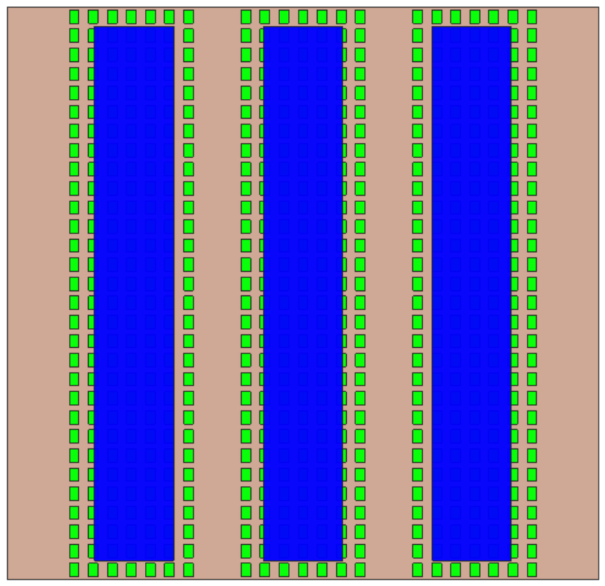
The worst-plant relative yield is the smallest season-accumulated ratio between the yield of an individual plant under the array and the yield of the same position in the panel-free baseline. It is reported because a plot-mean ratio can satisfy a yield mandate while a sub-population fails it. The fifth percentile of the per-plant distribution is reported alongside the minimum, because with 630 plants, the minimum is an extreme order statistic, and the end rows of the plot are not fully covered by the array, as Section 3.2 describes.

The worst plant is an extreme value, so it is fair to ask whether it stands alone. For the six modes whose complete plant-level distribution was archived, the fifth percentile of the 630 relative yields lies within 3.3 percentage points of the worst plant in every case, and within 1.2 points in the closest one. The worst plant is therefore the edge of a dense lower tail and not an isolated outlier, which is what makes it usable both as a reported statistic and as an optimization constraint.

2.6.2. Land Equivalent Ratio

The Land Equivalent Ratio (LER) follows the intercropping definition of Mead and Willey [30]. Its transfer to systems with a non-agricultural co-product is discussed in the agroforestry literature [31,32] and in the geospatial assessment of elevated agrivoltaics of Willockx et al. [33]. The agrivoltaic form used here is that of Elamri et al. [34]:

$$LER ={\displaystyle \frac{Y_{\mathrm{APV}}}{Y_{\mathrm{ref}}}} + {\displaystyle \frac{E_{\mathrm{APV}}}{E_{\mathrm{ref}}}}$$

(10)

$Y_{\mathrm{ref}}$ is the cumulative yield of the panel-free baseline on the same plot. $E_{\mathrm{ref}}$ is the cumulative energy of a photovoltaic-only reference plant on the same land polygon. That reference is laid out by the same framework with the same module type, which on the demonstration plot means the same three rows on the same land polygon, generating 67.3 MWh over the simulated season. Two consequences follow and are stated here because they bound the interpretation of the ratio. First, the geometric penalty between the two layouts is small: once the loss factors of Section 3.1 are applied to both, the residual difference attributable to inter-row shading is 0.36%, a value consistent with the low ground cover ratio of the layout and with the inter-row spacing and shading-loss formulations of Appelbaum and Aronescu [35] and Varga and Mayer [36]. Second, the soiling and degradation factors are applied to the agrivoltaic array but not to the reference, the former following the linear accumulation with rainfall reset of Kimber et al. [37] as refined by Coello and Boyle [38] and Redondo et al. [39], whose techno-economic consequences are reviewed by Ilse et al. [40] and which has been measured on an agrivoltaic installation by Jung et al. [41], so the reported energy sub-ratio contains a loss term that the reference does not carry; applying the same factors to the reference reduces it to 57.2 MWh. The energy sub-ratio therefore measures the fraction of a dedicated solar plant that the agrivoltaic array delivers on the same land, under a loss treatment that the reference does not carry, and the two sub-ratios are reported separately for that reason. The two terms of the ratio respond to the tracking angle in opposite directions, so their sum can conceal that behavior.

2.6.3. Avoided Carbon Dioxide

The avoided carbon dioxide is the sum over the season of the energy generated of each step multiplied by the grid carbon intensity of that step. Curtailed energy is not counted as avoided.

2.6.4. Net Global Balance

The net global balance is the seasonal sum of the energy revenue, evaluated through the dispatch cascade of Section 2.5.1, plus the value of the harvested crop, minus the operation and maintenance cost prorated over the simulated days. The capital cost is not prorated onto the season, because a seasonal capital charge would dominate the balance without conveying project-level information. The balance is therefore an operating indicator for the comparison of modes, and not a project-level profitability indicator.

2.7. The Crop Growth Response and Validation Status of the Physical Evaluator

Because the interior optimum of the yield response is the property on which several of the modes depend, the crop response computed by the evaluator is stated here in full before its validation is reported. The gross dry-matter growth of one plant over one hourly step follows the radiation use efficiency form of Monteith [42]:

$$G = {\mathrm{PAR}}_{\mathrm{eff}} · f_{\mathrm{int}} · \mathrm{RUE} · K_w · K_s$$

(11)

where $f_{\mathrm{int}}$ is the canopy light-interception fraction, $\mathrm{RUE}$ is the radiation use efficiency in grams of dry matter per megajoule of photosynthetically active radiation, and $K_{\mathsf{w}}$ and $K_{\mathsf{s}}$ are dimensionless water and thermal stress factors, each bounded between zero and one. The photosynthetically active radiation is a fixed fraction of 0.487 of the shortwave irradiance reaching the plant, the multiplier that Zhu et al. [43] apply for the same purpose. The same expression is applied to the agrivoltaic plant and to its panel-free baseline twin, so every factor that is common to the two zones cancels in the ratio that Section 4 reports.

The saturating response to light is carried by the first factor, a rectangular hyperbola relative to the full-sun radiation of the same hour. It preserves the initial slope of [42] in the light-limited regime and saturates above it, an inflection that Zhu et al. [43] place at about one-quarter of full sunlight and that the reference trial itself reports for these species [6]:

$${\mathrm{PAR}}_{\mathrm{eff}} = {\mathrm{PAR}}_{\mathrm{ref}} · \mathrm{PAR}/(\mathrm{PAR} + k_{\mathrm{sat}} · {\mathrm{PAR}}_{\mathrm{ref}})$$

(12)

in which $\mathrm{PAR}$ is the radiation reaching the plant under the array and ${\mathrm{PAR}}_{\mathrm{ref}}$ is the radiation reaching the baseline plant in the same hour, so that the baseline evaluates the expression at $\mathrm{PAR} = {\mathrm{PAR}}_{\mathrm{ref}}$.

The thermal factor $K_s$ is a trapezoidal response on four cardinal temperatures, the form common to DSSAT [44] and to AquaCrop [45], evaluated here on the infrared canopy temperature of each plant: it equals one between $T_{\mathrm{opt},\min }$ and $T_{\mathrm{opt},\max }$, falls linearly to zero at $T_{\min }$ below and at $T_{\max }$ above, and rises under the array because the canopy there is cooler.

The water factor $K_{\mathsf{w}}$ is the water-stress coefficient of FAO-56 [28]:

$$K_{\mathsf{w}} = \left(\mathrm{TAW} - D_{\mathsf{r}}\right)/(\mathrm{TAW} - \mathrm{RAW})$$

(13)

with $\mathrm{TAW}$ the total available water, $\mathrm{RAW}$ the readily available fraction, and $D_{\mathsf{r}}$ the current root-zone depletion; shading lowers the radiative term of the evapotranspiration, hence the depletion, hence the stress.

The radiation use efficiency is not modified by shade in the runs reported here. The diffuse-enhancement and dry-matter-shift coefficients that the implementation admits are both zero in the bibliographic parameter set. The reported yield ratio is therefore a pure dry-matter ratio, and the relative yields above unity of Section 4 are produced by the saturating light response and by the two stress factors alone.

The parameter set for Salvia officinalis is given in

Table 2. Parameter set for Salvia officinalis. No value was fitted to the demonstration plot. “Assumed” marks a working value that is not taken from a published source for this species. The depletion fraction is adopted by analogy with the perennial Lamiaceae tabulated by Pereira et al. [46]. The last two rows are zero in the bibliographic parameter set, so the radiation use efficiency and the dry-matter fraction are identical in the two zones. Where a value could not be traced to a published source for this species, the table gives the reference that bounds it: [47] for the radiation use efficiency and the interception fraction, both set at or below the range that the review reports for field canopies on a photosynthetically active radiation basis; [28] for the wilting point; and [48] for the water content of the fresh harvest and the floor on the dry-matter fraction, which reports 75 to 80% moisture for fresh medicinal and aromatic plants. The allocation to the harvested organ has no published value for this species and is set on the basis that, in a leaf herb, the harvested organ is most of the above-ground biomass.

Symbol	Parameter	Value	Source
$\mathrm{RUE}$	$\mathrm{Radiation} \mathrm{use} \mathrm{efficiency} (\mathrm{g} {\mathrm{M}\mathrm{J}}^{-1}$$\mathrm{of} \mathrm{PAR}$)	1.2	Assumed, [47]
$f_{\mathrm{int}}$	Canopy light-interception fraction	0.80	Assumed, [47]
$k_{\mathrm{sat}}$	Light saturation coefficient	0.40	[49]
$T_{\min }$	Lower temperature limit (°C)	5	[50]
$T_{\mathrm{opt},\min }$	Lower optimum temperature (°C)	15	[50]
$T_{\mathrm{opt},\max }$	Upper optimum temperature (°C)	26	[50]
$T_{\max }$	Upper temperature limit (°C)	30	[50]
$P$	Soil water depletion fraction for no stress	0.45	[46]
$f_{\mathrm{WP}}$	Wilting point as a fraction of root-zone capacity	0.54	Assumed [28]
$f_{\mathrm{harvest}}$	Allocation to the harvested organ	0.75	Assumed
$\mathrm{DM}$	Dry-matter fraction of the harvested fresh weight	0.20	Assumed, [48]
${\mathrm{DM}}_{\min }$	Floor on the dry-matter fraction	0.15	Assumed, [48]
$k_{\mathrm{diff}}$	Diffuse-enhancement coefficient of the $RUE$	0	Section 2.7
$C_{\mathrm{W}}$	Dry-matter-shift coefficient	0	Section 2.7

.

The structure of the ratio identifies which of these coefficients can move the interior optimum. Since $\mathrm{RUE}$ and $f_{\mathrm{int}}$ are identical in the two zones (agrivoltaic and baseline), they cancel exactly and cannot displace it. The optimum is therefore located by $k_{\mathrm{sat}}$, which sets how cheaply light can be given up, and by the upper edge of the thermal window, $T_{\mathrm{opt},\max }$, and $T_{\max }$, which sets how much is gained by cooling the canopy. The depletion parameters act in the same direction as the thermal window but through a slower state variable. A quantitative sweep of these coefficients is listed among the future directions of Section 6.

The crop-coupling sub-models were compared against two field campaigns carried out on the same dynamic single-axis geometry that is adopted here, over six aromatic species in southern Italy [5,6]. Sage is one of those six species, so the crop of the present demonstration lies inside the tested set and is not an extrapolation to a different species. The comparison uses relative, offset-cancelling metrics; that is, under-panel to full-sun ratios and thermal differentials on a representative interior sample. Relative metrics are used because the reanalysis forcing and the on-site handheld radiometry differ by about 30% in absolute level, and a ratio cancels an offset that is common to both zones. The parameter set used in that comparison is the bibliographic set used here, and not a set fitted to the trial.

Table 3. Validation and verification status of the physical evaluator. The crop rows come from the field campaigns of the same tracker geometry [5,6] with the bibliographic parameter set. The photovoltaic row comes from a code-to-code verification against an independent implementation over the 3672 hourly steps of the simulated season.

Quantity	Simulated	Measured	Agreement
Under-panel to full-sun yield ratio, sage	0.576	0.622	Difference −0.046
Under-panel to full-sun yield ratio, six aromatic species	-	-	MBE +0.01, RMSE 0.154, Spearman ρ 0.37
Under-panel to full-sun shortwave ratio	0.120	0.128	Difference −0.008
Canopy infrared depression under the panels (°C)	−1.70	−2.40	Difference +0.70
Hourly photovoltaic energy against pvlib python	-	-	MBE +0.03%, r 0.972, maximum monthly deviation 0.52%

reports the outcome.

The reference trial reports no electrical output, so the photovoltaic chain cannot be validated against it. That chain was therefore verified code-to-code against an independent open-source implementation, pvlib python (version 0.15.2) [51], driven by the same hourly meteorological series and the same array configuration. Over the 3672 steps of the simulated season, the mean bias error on hourly energy is +0.03%, the hourly correlation is 0.972, and the largest monthly deviation is 0.52%. The agreement statistics reported in Table 3 follow the model-evaluation guidance discussed in Section 5.3, which favors the mean bias error over normalized coefficients at small sample size.

Three limits should be read together with these numbers. First, the agronomic comparison establishes the model as an unbiased constraint on the magnitude and the direction of the shade response, and not as a fine ranking predictor across species: the rank correlation over the six species is 0.37, and five of the six species cluster within a narrow band of yield reductions, which makes any normalized coefficient unstable on this sample. Second, the code-to-code verification tests the transposition, thermal and conversion sub-models, and does not test the inter-row shading of the agrivoltaic layout, for which no independent reference is available here. Third, the operating layer itself is not validated against a plant that has been operated under any of the nine modes. The modes are therefore compared against each other under identical drivers, which is the comparison that Section 4 reports.

2.8. Solver Settings and Reproducibility

The nine modes share one solver and one set of settings and differ only in how the two available searches are combined, so that the differences of Section 4 come from the objectives and the constraints and not from the numerics. The framework and the nine mode implementations are written in MATLAB (version R2025a, The MathWorks, Inc., Natick, MA, USA). The gradient search is a sequential quadratic programming implementation, limited to 30 iterations and 105 function evaluations per step, with an optimality tolerance and a constraint tolerance of 0.001, a step tolerance of 0.01 and forward finite differences of 0.01°; Mode 8 uses the same scheme with the iteration limit set to 10. The discrete search is a scan of the admissible range at a spacing of 5°, with the number of points forced odd so that the horizontal orientation always falls on the grid, which gives 19 points over the mechanical range of ±45° of this plot. Mode 1 is solved by the scan alone, seeded from the closed-form tracker orientation. Modes 3, 4, 7 and 8 run both searches at every step and keep the better candidate, so their reported solution is never worse than the gradient one. Modes 2 and 5 run the gradient search and call the scan on the branch in which the constraint is relaxed. Modes 6 and 9 run the gradient search alone from several deterministic starting points, because their objectives are two-phase or constrained in a way that a single scan of a scalar angle does not resolve.

The comparison is not decorative. Over the 2176 optimized steps of the pure-yield mode, the scan strictly improves on the gradient solution in 1898 steps; that is, 87%, and the two agree exactly in the remaining 278. The improvement is negligible at most steps, with a median of five parts in ten million, but it exceeds 1% of the objective at 41 steps and 10% at four of them, which is where a local method on a non-smooth objective would otherwise have been trapped. The energy tie-break of Modes 3 and 4 settles the choice at 860 of those same steps, and at every one of them, the yield objective differs between the two candidates by less than five parts in one hundred million, so it resolves indifference rather than competing with the crop.

No part of the optimization is stochastic. There is no random seeding, no multi-start from random points and no population-based search in any of the nine mode implementations. The starting points are the analytical orientation of the step, the position held at the previous step, and the limits of the admissible range, all of which are determined by the state of the simulation. Repeating a run with the same drivers, the same configuration and the same code version therefore reproduces the reported figures exactly, and the verification runs described in Section 5.1 were carried out on that basis.

The cost of a run follows from the same structure. Every candidate orientation evaluated by either search applies the angle to all panels and then recomputes the projected shadows, the sky view factor, the net radiation and the yield of all 630 plants, so the cost scales approximately with the product of the number of plants, the number of panels and the number of steps, and is dominated by the polygon operations of the shading geometry. Only the evapotranspiration and the resulting soil water state are not recomputed inside the step and are carried from the previous hourly state, an approximation that is admissible because the optimization takes place within a single hourly step. At field scale, on the order of a thousand trees and a few thousand modules, the same chain costs several wall-clock hours per simulated day on a single-thread workstation, with the constrained modes at the upper end because the chain is evaluated inside the non-linear constraint at every solver iteration. On the demonstration plot, which carries three modules, a full season of 3672 steps takes between 16,000 and 21,000 s of wall-clock time; that is, between about four-and-a-half and six hours, with those same modes at the upper end of the range. The framework is accordingly a design and parametric-study tool and not a real-time controller.

One qualification on reproducibility belongs here, because it follows from the shape of the crop objective rather than from the numerics. For the modes that maximize the yield metric, the objective is very nearly symmetric about the horizontal orientation: at many steps the two extreme tracking angles differ in the objective by a few parts in one hundred million, so which of them is selected is decided at the level of floating-point arithmetic, and the choice then propagates through the accumulated state. An independent re-execution of Mode 3 on a later build of the simulator, with the same drivers and the same configuration, reproduces 67% of the hourly orientations of the reported run step by step, and reproduces the seasonal aggregates to within 1.8% in photovoltaic energy, 1.3 percentage points in mean relative yield and 0.07% in Land Equivalent Ratio. The eight remaining modes do not show this behavior, because their objectives vary with the angle by percentage points. The near-symmetry is a property of a plot in which the two extreme tracking angles shade the canopy almost equally over the season, and the tolerance quoted here applies across builds of the code rather than to a repetition under identical conditions.

The large language model Claude (version Opus 4.8, Anthropic, San Francisco, CA, USA) was used to improve the quality of the English writing and to assist in the debugging and verification of the simulation and analysis code. All output was reviewed, tested, and edited by the authors.

3. Case Study Configuration

The case study is a demonstration vehicle. Its purpose is to show that the nine modes give distinct and internally consistent operating points under identical conditions, and to measure the trade-off surface that they trace.

3.1. Plot and Photovoltaic Array

The photovoltaic hardware follows the dynamic single-axis installation of the Disciglio field trials [5,6]. The geometry is kept unchanged, but the plot is placed in Valencia, Spain, and is driven by Spanish meteorological, market and grid-carbon series. This separates the two sources of uncertainty. The geometry is the one for which measured shade responses exist, and the electrical drivers are the ones that apply to the market in which the plant would operate.

The land polygon is 30.95 m by 30.0 m; that is, 928.5 ${\mathrm{m}}^2$. The array has three parallel rows. Each row is a continuous string of opaque monofacial modules 4.15 m wide and 28.0 m long, mounted 2.5 m above the ground. Each row rotates about its horizontal axis, which is parallel to the row.

Table 4. Photovoltaic array and electrical parameters of the demonstration plot.

Parameter	Value
Land polygon	$30.95 \times 30.0 \mathrm{m} (928.5 {\mathrm{m}}^2$)
Number of rows	3
Module area per row/total	$116.2 {\mathrm{m}}^2$$/348.6 {\mathrm{m}}^2$
Rated capacity per row/total	22.0 kWp/66.0 kWp
Nominal power density at standard test conditions	$189 \mathrm{Wp}/{\mathrm{m}}^2$(18.9% module efficiency)
Clear height above ground	2.5 m
Row pitch/clear distance between rows	8.85 m/4.70 m
Ground cover ratio (row pitch basis/land basis)	0.47/0.38
Tracking axis	Horizontal, parallel to the row
Mechanical range	±45° from horizontal
Slew limit	90° per hourly step
Module type	Opaque, monofacial
Derating factor	0.85
Reference irradiance/cell temperature	$1000 \mathrm{W}/{\mathrm{m}}^2$/25 °C
Temperature coefficient of power	−0.34%/°C
Cell temperature model	$\mathrm{Faiman}, U_0=25{\displaystyle \frac{\mathrm{W}}{{\mathrm{m}}^2\mathrm{K}}},{ U}_1=6.84{\displaystyle \frac{\mathrm{W}·\mathrm{s}}{{\mathrm{m}}^3 \mathrm{K}}}$
Capital cost	1200 EUR/kWp
Operation and maintenance cost	30 EUR/kWp per year

gives the electrical parameters.

All energy results in Section 4 refer to the installed capacity of 66.0 kWp.

Two loss mechanisms act on the array and enter every energy figure of Section 4 and the energy sub-ratio of Section 2.6.2. Soiling accumulates linearly at 0.15% per day up to a ceiling of 15% and is reset by any daily rainfall above 5 mm, following the formulation cited in Section 2.6.2; no manual cleaning is scheduled. The simulated season received 1.1 mm of rain in total, so the reset threshold was never reached and the soiling loss ran for the whole of the 153 days until it saturated at its ceiling. Module degradation is applied at 0.5% per year from a commissioning date of 1 January 2015. Both factors are applied to the agrivoltaic array and not to the photovoltaic-only reference of Section 2.6.2, and that asymmetry is quantified there.

3.2. Crop Layout and the Worst-Plant Statistic

The plot holds 630 sage plants on a regular grid of 30 rows by 21 columns, spaced 1 m in both directions. The 21 columns form three planted bands of seven columns. Each band spans 6.0 m from its first to its last plant column and is centered on one photovoltaic row, so the band pitch equals the row pitch of 8.85 m, and the clear distance between the last plant column of one band and the first column of the next is 2.85 m. Figure 2 shows the layout.

Because the modules are 4.15 m wide, their footprint at the horizontal orientation covers about four of the seven columns of a band. At the ±45° mechanical limits, the horizontal projection of a module narrows to 2.93 m and covers about three columns. The planted grid is 29.0 m long, and the modules are 28.0 m long, so the first and the last plant row extend 0.5 m beyond the ends of the modules.

The layout therefore contains three different shade populations within one plot: plants that are shaded through most of the day, plants that are shaded intermittently, and plants that are almost never shaded. This is what makes the worst-plant statistic meaningful. Each mode is judged on the least favored plant as well as on the plot mean.

The crop is sage (Salvia officinalis). It is parameterized through the external and interchangeable parameter set. The crop coefficients follow the seasonal curve applied to the same species in the reference trial, rising from 0.40 at the start of growth in April to 0.95 at full production in July and August, with a seasonal mean of 0.74 [6], and they enter the water-balance procedure of FAO Irrigation and Drainage Paper 56 [28]. The ancillary parameters of that balance—that is, maximum crop height, rooting depth, depletion fraction for no stress and fraction of ground cover—are adopted by analogy with the perennial Lamiaceae of the same functional group tabulated by Pereira et al. [46], because no crop-coefficient curve determined for Salvia officinalis has been published: that review tabulates rosemary, common thyme, oregano, mint, summer savory, lemon balm and lavender, but not sage. The remaining phenological, cardinal-temperature and shade-response values are literature-based. Table 2 gives the full parameter set with the source of each value. This bibliographic parameter set was not fitted to the case study. It is therefore the appropriate choice for a plot at a different location.

Sage is used because its moderate shade response makes the yield objective an active competitor of the energy objective. Disciglio et al. [6] measured a seasonal mean daytime irradiance of 85 W/${\mathrm{m}}^2$ under the panels against 662 W/${\mathrm{m}}^2$ in the full-sun control, and a sage fresh weight at harvest of 468 g per plant against 753 g in the control plot. Sage therefore retained about 62% of its full-sun fresh weight under a radiation reduction of about 87% [5]. A shade-neutral crop would leave the yield-driven modes almost indistinguishable from pure energy maximization. A shade-intolerant crop would align the yield optimum with the energy optimum. Sage sits between these limits, which is why it exposes the trade-off. The possibility that moderate shade raises rather than lowers production in a Mediterranean summer is supported by shading-net experiments on woody crops, in which canopy temperature falls and photosynthetic performance improves during heat events [52,53,54]. The temperature-response formulation used for the heat stress coefficient follows the comparison of routines of Liu et al. [55], and the use of canopy temperature as a stress indicator follows Jackson et al. [56]. The crop remains a constraint and a co-product here, and not the quantity being scheduled.

3.3. Meteorological, Market and Grid-Carbon Drivers

The meteorological input is the Open-Meteo hourly reanalysis for the Valencia site (39.474° N, 0.380° W, 150 m above sea level) for the year 2025. The simulated season is 1 April to 31 August 2025, which is 3672 hourly steps.

The electrical drivers are the Spanish hourly series for the same period: the regulated buy price applicable to the farm, the price paid for exported surplus, and the national grid carbon intensity.

Table 5. Statistics of the electrical drivers over the simulated season (1 April to 31 August 2025, 3672 hourly steps). Solar hours are the hours with a global horizontal irradiance above 50 W/${\mathrm{m}}^2$. The irradiance weighted mean is a proxy for the value that a photovoltaic plant captures.

Quantity	All Hours	Solar Hours	Midday (11:00–16:00)
Number of hours	3672	1950	918
Mean buy price (EUR/kWh)	0.125	0.122	0.087
Mean sell price (EUR/kWh)	0.050	0.032	0.013
Hours with sell price at or below zero	715 (19.5%)	712 (36.5%)	517 (56.3%)
$\mathrm{Mean} \mathrm{grid} \mathrm{carbon} \mathrm{intensity} (\mathrm{g}\mathrm{C}{\mathrm{O}}_2$/kWh)	81.4	68.0	60.5
Irradiance-weighted mean sell price (EUR/kWh)	0.024	-	-
Irradiance-weighted mean carbon intensity (gCO2/kWh)	65.0	-	-

gives their statistics. These series are the reason why the operating objective matters, so their structure is stated before the results.

Two properties of Table 5 govern the results of this paper.

• First, the value of a generated kilowatt-hour collapses in the hours of highest generation. Over the season, 715 h have a sell price at or below zero, and 517 of them fall in the six midday hours. The irradiance-weighted mean sell price is 0.024 EUR/kWh, which is 48% of the plain hourly mean, so a photovoltaic plant on this site captures less than half of the average market value of its energy. Over all hours the buy price is 2.5 times the sell price; restricted to the midday window, where most of the generation falls, it is close to seven times. Self-consumption is therefore worth far more than export exactly when the array produces most. The buy price itself falls at midday, from 0.125 to 0.087 EUR/kWh, because the regulated tariff follows the same wholesale collapse, so midday self-consumption is worth less than evening self-consumption but still far more than midday export.
• Second, the grid carbon intensity moves in the same direction. Over the season it correlates with global horizontal irradiance at −0.50. The irradiance-weighted mean is 65.0 gCO₂/kWh against a plain mean of 81.4 gCO₂/kWh, so midday photovoltaic energy displaces an already low-carbon grid.

The community tier of the dispatch cascade of Section 2.5.1 is not populated in this single-plot demonstration. The crop co-product is valued at 2.00 EUR/kg of fresh matter, which is the reference price of the dried aromatic product. This price is the single parameter that positions Modes 5 and 8 on the energy-to-crop axis. Section 5.3 states the limits that it places on the economic conclusions, and identifies which findings are independent of it.

One accounting convention should be stated before the results. In the hours when the sell price is negative, exported energy earns no revenue, and every mode with an economic objective responds by turning the array away from its energy optimum. Mode 5 is reported under a physical shutoff convention: the energy generated in those hours is treated as curtailed and is excluded from its seasonal photovoltaic total and from the avoided carbon dioxide computed from that total. The remaining eight modes report all the energy they generate. The energy and carbon columns of Mode 5 in

Table 6. Seasonal summary of the nine modes on the sage plot: photovoltaic energy, plot-mean relative crop yield, worst-plant relative yield, Land Equivalent Ratio with its energy sub-ratio in parentheses, pumping energy, avoided carbon dioxide, and net global balance. The photovoltaic energy, the avoided carbon dioxide and the energy sub-ratio of Mode 5 follow the curtailment convention stated at the end of Section 3.3.

#	Mode	PV Energy (MWh)	Rel. Yield (%)	Worst Plant (%)	LER (E-sub)	Pump (kWh)	Avoided $\mathbf{C}{\mathbf{O}}_2$ (kg)	Net Balance (EUR)
1	Electrical energy	57.04	95.1	60.7	1.799 (0.848)	32.30	3738	1676
2	Electrical energy under yield floor (80%)	55.71	105.2	88.8	1.880 (0.828)	32.75	3656	1789
3	Yield	53.54	109.3	94.4	1.889 (0.796)	34.87	3519	1775
4	Yield under electrical energy floor	53.93	108.1	93.2	1.882 (0.801)	34.31	3531	1742
5	Economic benefit	31.89	95.8	62.3	1.432 (0.474)	32.39	2121	1733
6	Electrical demand-following	45.07	102.6	85.5	1.695 (0.670)	32.70	2935	1404
7	Net $\mathrm{C}{\mathrm{O}}_2$ (adaptive) (thr. 80)	54.00	106.4	91.9	1.866 (0.803)	34.22	3562	1760
8	Economics–$\mathrm{C}{\mathrm{O}}_2$ Pareto	56.39	106.5	92.1	1.903 (0.838)	34.01	3699	1816
9	Crop-water minimization	55.78	102.6	81.1	1.854 (0.829)	32.54	3660	1742

are therefore conditional on this convention, whereas its yield statistics and its net balance are not, because energy exported at a negative price earns nothing under either treatment. The Land Equivalent Ratio of Mode 5 follows the same convention in its numerator, while its denominator stays the uncurtailed photovoltaic reference of Section 2.6.2, which is held identical across the nine modes so that the column can be read from top to bottom.

4. Results

The nine modes were applied to the sage plot over a full growing season (1 April–31 August), under identical geometry, meteorology, market and grid-carbon series, so that only the objective differs across modes. Every seasonal figure reported here is the outcome of composing the hourly policy of a mode over the season, and not an optimum with respect to the accumulated metrics; Section 5.1 measures the difference between the two. Table 6 gives the seasonal summary. The panel-free baseline consumed 37.9 kWh of pumping energy over the season, against which every mode reported.

The nine modes are distinct on every reported indicator. Photovoltaic energy spans 25.2 MWh, plot-mean yield spans 14.2 percentage points, worst-plant protection spans 33.7 percentage points, the Land Equivalent Ratio spans 0.47, and the net balance spans 412 EUR. No two modes coincide across the full indicator set, although Modes 4 and 9 return the same net balance, which supports the first part of the hypothesis of Section 1.

4.1. The Electrical Energy and Yield Trade-Off Surface

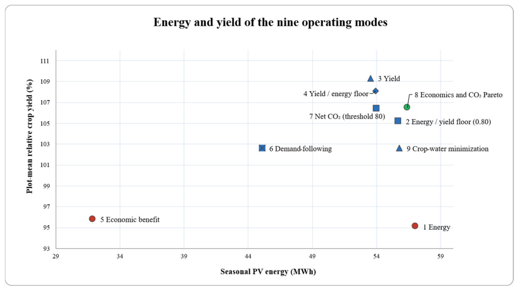
Figure 3 places the nine modes on the energy and yield plane. The energy-maximizing Mode 1 sits at the high-energy and low-yield corner, with a plot-mean yield of 95.1% and a worst plant that falls to 60.7%. The economic Mode 5 shares this weak crop protection, at 95.8% and 62.3%, and it delivers the lowest energy of all modes, 31.89 MWh, because it shuts generation down whenever the sell price is negative. The crop-driven Modes 3 and 4, the adaptive carbon Mode 7 and the Pareto Mode 8 occupy the opposite corner. They trade between 0.7 MWh and 3.5 MWh of energy for a plot-mean yield above 106% and a worst plant protected to between 92% and 94%.

The central result of the case study is that Mode 1 sits at a flat extreme of the trade-off frontier. It is Pareto-optimal by construction, because no mode delivers more energy, but the frontier is almost flat next to it, so energy maximization is a poor operating choice. Mode 8 gives 11.4 percentage points more plot-mean yield and 31.4 percentage points worst-plant protection than Mode 1, and it costs only 0.65 MWh; that is, 1.1% of the energy. The reason is geometric. The energy response is flat near its peak, because it varies with the cosine of the deviation from the sun-pointing angle, while the ground shadow pattern moves approximately linearly with that deviation. A small departure from the sun-pointing angle therefore buys a large change in the radiation reaching the canopy at almost no energy cost.

Past that point the trade-off becomes expensive. From Mode 8 to the pure-yield Mode 3, a further 2.8 percentage points of yield cost 2.85 MWh. The marginal cost of yield rises from 0.057 MWh per percentage point to 1.018 MWh per percentage point; that is, by a factor of about 18. The energy and yield surface therefore has a well-defined knee, and Mode 8 sits on it.

The plant-level distribution of the pure-yield mode shows where the crop response turns. Over the hours with appreciable sun, the mean fraction of the plant that lies in the geometric shadow of a module ranges from 0.9% to 50.5% across the 630 plants, and the seasonal shortwave radiation that each plant receives ranges from 0.433 to 0.976 of that received by its baseline twin. The radiation deficit exceeds the beam shadow fraction in every case, because the array also reduces the diffuse component through the sky view factor. The final relative yield ranges from 0.944 to 1.262, and 503 of the 630 plants finish above the full-sun reference. The ratio crosses unity at about 0.89 of the full-sun radiation and rises to a broad interior maximum near 1.17 between 0.5 and 0.7 of it. The response is therefore not monotone in the shading: the least-shaded plants lose light without gaining enough thermal relief to compensate, and the most-shaded ones begin to give the gain back. This is the interior optimum of Section 2.1 measured on the plot.

Mode 2, which maximizes energy subject to the 80% accumulated worst-plant floor, sits between Mode 8 and Mode 1 on energy, at 55.71 MWh, while it holds its worst plant at 88.8%. The accumulated floor is banked early in the season, and the worst-plant ratio then climbs with summer growth, so it settles well above the nominal 80% target. The practical consequence is favorable for an operator under a yield mandate: compliance with a floor that is well above the German threshold costs 2.3% of the seasonal energy.

Mode 6 curtails generation to 45.07 MWh; that is, 12.0 MWh below Mode 1, in order to follow the demand set-point. This is the expected demand-following signature, and it is the price of matching a load without storage.

4.2. Economics and the Value of the Exported Kilowatt-Hour

The net balance does not rank the modes in the order of their energy. Mode 1 produces the most energy of all modes and ranks eighth of nine on the balance, at 1676 EUR. Mode 5 produces 44% less energy than Mode 1 and still returns a higher balance, 1733 EUR. Mode 8 attains the highest balance of all modes, 1816 EUR, ahead of Mode 2 at 1789 EUR and of the pure-yield Mode 3 at 1775 EUR.

Two mechanisms produce this ordering, and they must be separated:

• The first is the price structure of Table 5. Mode 5 curtails at negative prices and prioritizes self-consumption, so the megawatt-hours that it does generate are worth much more than the average megawatt-hour of Mode 1. This is a purely electrical effect, and it is the operational expression of the value migration described in Section 3.3. Its magnitude is visible directly in Table 6: Mode 5 generates 25.15 MWh less than Mode 1, that is 44% less, and still returns 57 EUR more.
• The second is the crop co-product. At the assumed price of 2.00 EUR/kg, the crop term dominates the plot economics, so modes that protect the crop earn more than a mode whose hourly objective is biased toward electricity that is worth little at midday. This identifies the crop, and not the electricity, as the dominant economic driver of this plot at this price. Section 5.3 states the limits of that conclusion.

Mode 5 ranks seventh of the nine modes even though the economic benefit is its objective. This follows from the valuation split described in Section 2.5.1. The objective is optimized on the stable reference proxy, whereas the reported balance is anchored on the final harvest. Mode 5 therefore ends 83 EUR below the best-performing Mode 8; that is, 4.6% of that balance. This difference measures the ranking penalty of the valuation split, and not the size of the split itself.

Mode 5 also avoids the least carbon dioxide of all modes, 2121 kg, because the curtailed midday energy is not exported. The physical shutoff treats that surplus as worthless, because the grid price is negative. Within an agricultural energy community, however, the energy generated at negative prices need not be curtailed at all. It could be allocated to member loads or to storage rather than exported at a loss, which is an energy-allocation problem addressed by the hybrid static-dynamic community model of [57].

4.3. Carbon: The Degeneracy and the Adaptive Switch

The avoided carbon dioxide per megawatt-hour generated is 65.5 kg for Mode 1, 65.6 for Mode 2, 65.7 for Mode 3, 65.5 for Mode 4, 66.5 for Mode 5, 65.1 for Mode 6, 66.0 for Mode 7, 65.6 for Mode 8 and 65.6 for Mode 9. The whole spread is 2.1% around a mean of 65.7 kg/MWh, and that mean coincides with the irradiance-weighted grid carbon intensity of 65.0 gCO₂/kWh reported in Table 5.

This is direct numerical evidence for the structural claim of Section 2.1. The orientation moves the avoided carbon dioxide almost only through the energy that it generates, and not through the carbon value of the hours in which it generates, so an objective that minimizes net carbon dioxide through the orientation alone is degenerate with the energy objective on this grid series. Modes 7 and 8 exist to break that degeneracy, and they are the reason the paper does not report a tenth mode that maximizes avoided carbon directly. The degeneracy is a property of a grid whose hourly carbon intensity is anti-correlated with solar output and varies little within the generating hours, and not of the method: on a grid with a larger hourly spread, the same carbon objective would be non-degenerate, and the framework would optimize it directly.

Mode 7 breaks it with the hard switch. At the 80 gCO₂/kWh threshold, it lands in the crop-protecting cluster, at 54.00 MWh, 106.4% yield and a worst plant at 91.9%, and not near the energy corner. Because solar output and grid carbon intensity are anti-correlated, the clean branch is active in 2035 of the 3672 h and covers 81% of the seasonal generation, so the crop branch governs the high-output midday core while the energy branch is confined to the low-output morning and evening hours. Raising the threshold to 90 gCO₂/kWh extends the clean branch to 2499 h but moves the operating point very little, to 53.7 MWh and 108.1% yield, because the hours that change branch carry little irradiance. Mode 7 is therefore stable across the two thresholds tested near the grid mean, and it is a genuinely crop-favoring operating point rather than a relabeled Mode 1. A full sweep of the threshold is left to a dedicated study.

Mode 8 breaks the degeneracy softly and reaches the highest Land Equivalent Ratio of all modes, 1.903, together with the highest balance. It settles at an interior orientation, near a midday tracking angle of 29°, and not at either single-objective corner.

That value sits above the range most often reported in the literature. The PRISMA-based systematic review of Martinez-Hernandez et al., which synthesizes 249 studies published between 2010 and 2025, places typical Land Equivalent Ratio values between 1.2 and 1.8 [58]. Two properties of this plot explain the difference, and neither of them is a weakness of the reference. The agricultural sub-ratio exceeds unity, 1.065, because a moderately shade-tolerant species is operated under a policy that protects it, whereas most of the reviewed installations report an agricultural sub-ratio below unity. The energy sub-ratio, 0.838, is in fact modest, and the low ground cover ratio of this layout is what allows the agricultural term to stay above one. The value reported here is also an operating-point indicator obtained under a specific hourly orientation policy over one season, and not an installation-level average, so it should be compared with the reviewed range as an upper operating bound rather than as a like-for-like measurement.

4.4. The Electrical Demand-Side Water Lever

Mode 9 treats the panel orientation as a demand-side resource. By shading the canopy, it lowers the radiative term of the evapotranspiration, hence the irrigation volume and the pumping energy.

The lever is real but small, and it is close to saturation. The panel-free baseline consumed 37.9 kWh of pumping energy over the season. Every mode reduced this, to between 32.30 kWh for Mode 1 and 34.87 kWh for Mode 3; that is, by between 14.8% and 8.0%. The full span across the nine modes is 2.57 kWh, which is 6.8% of the baseline and 0.005% of the seasonal photovoltaic generation. The presence of the array delivers most of the saving. The orientation then redistributes a small residue.

Mode 9 reached 32.54 kWh, a reduction of 14.1%. This is not the lowest value in Table 6. Mode 1 reached 32.30 kWh, a reduction of 14.8%. The reason is that Mode 9 carries the same 80% per-plant yield floor as Mode 2, which is the constrained optimum described in Section 2.4.4. The comparison of the two modes is therefore informative rather than contradictory. For 0.24 kWh of additional pumping energy and 1.26 MWh of photovoltaic energy, Mode 9 raises the worst-plant protection from 60.7% to 81.1% and the plot-mean yield from 95.1% to 102.6%. In an operating context, Mode 9 is best read as a water-aware crop-protection mode, and the orientation should not be presented as a primary instrument for irrigation-energy management at this site.

The bound is physical. Only the radiative term of the FAO-56 evapotranspiration responds to the tilt, and the aerodynamic term does not, so the achievable reduction is limited from below by an aerodynamic floor that is nearly reached once any shading is applied. The result therefore bounds the lever for this geometry and this climate and not for agrivoltaic irrigation in general: a plot with a larger pumping head, a deeper water table or a more water-demanding crop would place the same relative saving on a much larger absolute demand, and only there would the orientation become a material demand-side instrument.

5. Discussion

5.1. Non-Degeneracy of the Trade-Off Geometry

The central methodological claim is that a genuine trade-off between an energy-proportional objective and the energy itself requires either an objective with an interior optimum in the tracking angle, or a rule that changes the objective when the marginal kilowatt-hour loses its value. The framework provides both. Mode 8 supplies the interior optimum through the crop co-product. Mode 7 supplies the rule.

The season-long results support the hypothesis on both sides. The near-constant avoided carbon per megawatt-hour of Section 4.3 confirms the degeneracy that the two modes are designed to break. The interior operating point of Mode 8, its highest-of-all Land Equivalent Ratio and its highest-of-all balance confirm that the crop co-product makes the trade-off non-degenerate rather than energy-collinear. The robustness of Mode 7 to its threshold confirms that the adaptive rule is not a disguised energy mode.

Two limitations bound the Mode 8 claim. First, the weighted-sum scalarization recovers only the convex regions of the Pareto surface, a limitation of the method rather than of the model, and one for which alternative generators of the Pareto surface exist [59]; any concave portions would need a different scalarization—for example, an ε-constraint formulation—to expose. Second, the optimizer acts per hour on a state inherited from the previous step, so the seasonal operating point that it traces is a myopic composition of hourly decisions and not a true seasonal Pareto optimum. Both are acceptable for an hourly design-stage tool, but neither should be overstated as global optimality.

The weight was swept over five values to test both endpoints of the scalarization against the single-objective modes they should reproduce.

Table 7. Weight sweep of Mode 8 over the same season and drivers as Table 6. The weight of 0.50 is the operating point reported there. Energy and carbon follow the reporting conventions of Section 3.

Weight	PV Energy (MWh)	Rel. Yield (%)	Worst Plant (%)	Avoided $\mathbf{C}{\mathbf{O}}_2$	Net Balance (EUR)
0.00	57.226	102.81	83.67	3750.0	1768.8
0.25	57.267	105.67	91.10	3753.6	1805.8
0.50	56.394	106.52	92.15	3699.4	1815.7
0.75	55.227	106.22	93.31	3628.2	1811.0
1.00	54.855	106.10	93.67	3605.3	1808.3

reports the outcome. At a weight of 0.50, the sweep returns the Mode 8 row of Table 6 to five significant figures, which confirms that the reported operating point is the one the formulation defines.

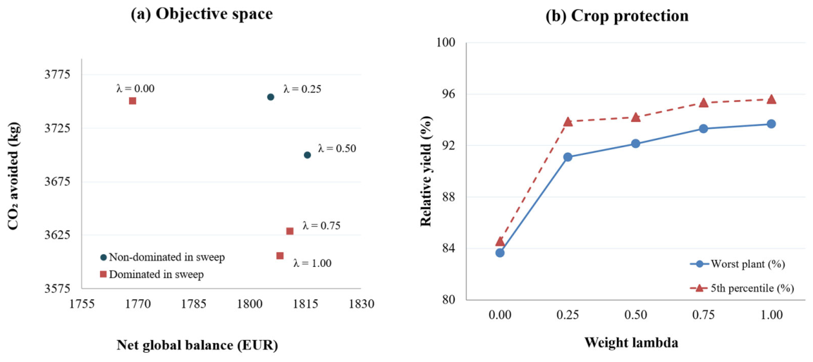
The endpoints behave differently, and in a way that is informative rather than anomalous. In the objective space of the scalarization—that is, the net balance against the avoided carbon dioxide—the weight of 0.25 attains more of both than the weight of 0, and the weight of 0.50 attains more of both than the weights of 0.75 and 1. Three of the five points are therefore dominated, and the two that survive are the interior ones. Since a weighted sum of two objectives cannot place its own endpoints inside the attainable set when the problem is separable, this is direct evidence that the hourly problem is not separable across steps.

Two distinct mechanisms produce that coupling, and they should not be conflated. The seasonal energy is a pure function of the orientation held at each step and does not depend on the state of the crop, because the canopy casts no shade on the array. The only channel through which the history of orientations can alter the seasonal energy is therefore the search itself, which is started from the position held at the previous step, so the local solution reached at one step depends on where the previous step left the array. That channel is worth 0.041 MWh, or 0.07% of the season. The seasonal balance is coupled through that channel as well, and additionally through the accumulated biomass and soil water state that carry the effect of earlier orientations into the later crop response. That combined channel is worth 7.45 EUR, or 0.41%, which is six times the energy-only effect.

The same sweep bounds the energetic reference of Mode 1. The highest seasonal energy reached anywhere in Table 7 is 57.267 MWh, against the 57.04 MWh of Mode 1 in Table 6, a margin of 0.40%. Mode 1 adopts the closed-form tracker orientation, which the sweep of Section 2.3.1 does not improve on at any step of this configuration, whereas the weight sweep refines the same per-step objective over the admissible range, so the margin measures the cost of the closed form and not a defect of the comparison. It is smaller than every difference between modes discussed in Section 4, so the ranking of Table 6 is unaffected.

The other endpoint warrants some discussion, because Section 2.5.3 states that a weight of 1 recovers Mode 5 while the two tables do not report the same figures for it. On energy, the two are not comparable, because Mode 5 is reported net of the curtailed hours under the convention of Section 3.3; on the common uncurtailed basis, Mode 5 generates 56.83 MWh against 54.86 MWh. On the net balance, the weight of 1 returns 1808 EUR against 1733 EUR, a margin of 4.3% that measures the difference between the two implementations of the same step objective, chiefly the feasibility and fallback machinery that Mode 5 carries and the weight sweep does not.

Read together, these results state the case for Mode 8 more strongly than the non-degeneracy argument alone. The sweep does not merely trace compromises that the single-objective modes already reach: at a weight of 0.25 the plot attains simultaneously the highest seasonal energy, the highest avoided carbon dioxide and the highest Land Equivalent Ratio of the whole study, 1.908, which follows from the columns of Table 7 through Equation (10), while holding the worst plant above 91%. The protection of the crop is meanwhile monotone in the weight over all five points, for the worst plant and for the fifth percentile alike, as Figure 4 shows, and almost all of the available protection is bought by the first quarter of agronomic weight at no cost on either objective.

5.2. Which Mode for Which Operator

The nine modes map onto distinct operator situations. Plots under an agrivoltaic yield mandate map onto Mode 2. Grid-tied self-consumption with a hard load guarantee maps onto Mode 4. Islanded or export-constrained demand matching maps onto Mode 6. Water-scarce sites map onto Mode 9. Market participation maps onto Modes 5 and 8. Carbon-signal-following operation maps onto Mode 7.

Three operational conclusions follow from Table 6 and are independent of the crop price:

• The first is that an operator who currently runs a tracker for energy alone is leaving crop protection on the table for almost nothing. The step from Mode 1 to Mode 8 costs 1.1% of the seasonal energy and raises the worst plant by 31 percentage points.
• The second is that regulatory compliance is cheap on this geometry. A per-plant floor of 80%, well above the 66% of DIN SPEC 91434 [29], costs 2.3% of the seasonal energy under Mode 2. The 90% floor of the French decree [60] is more demanding, as are the Italian guidance, the French assessment methodology, the Catalan technical instruction and the European best-practice guidelines [61,62,63,64]. Whether that floor is feasible for the worst plant on this geometry is an open question, and one the framework can answer directly.
• The third is that the per-plant resolution matters for enforcement. Because the yield floor is evaluated per plant rather than per plot, the framework diagnoses agronomic harm at the resolution at which national rules are properly enforced. The gap between the plot mean and the worst plant reaches 34.4 percentage points in Mode 1, so an aggregated ratio can hide a sub-population that fails the threshold while the plot appears compliant.

The same optimizer is intended to scale from the single plot to the collective level of an agricultural energy community. This would couple the plot-level dispatch presented here with a community energy-allocation and benefit-sharing layer such as the hybrid static-dynamic model of [57]. The unpopulated community tier of the dispatch cascade is the interface that this extension would use.

5.3. Limitations

The economic ranking is conditional on the crop price. The crop term of the balance scales linearly with that price while the energy term does not, so there exists a price below which the energy-favoring modes outrank the crop-favoring ones. The conclusion that the crop is the dominant economic driver is therefore a statement about this plot at 2.00 EUR/kg, and not a general result.

The switching prices can be stated exactly. The seasonal balance of each mode is the sum of an energy term net of operation and maintenance, which does not depend on the crop price, and a crop term equal to the harvested mass multiplied by that price. The harvested mass follows from the relative yield of Table 6 and a plot baseline of 574.86 kg, a value that six independent runs reproduce to six significant figures. Each mode is therefore a straight line in the crop price, and the best mode at any price is the upper envelope of nine such lines. Mode 8 holds that envelope between 0.66 and 4.54 EUR/kg. Below 0.66 EUR/kg the envelope passes to Mode 5, whose higher energy term then outweighs its lower crop term; above 4.54 EUR/kg it passes to the pure-yield Mode 3. The reference price of 2.00 EUR/kg lies inside a band that spans a factor of seven, so the ranking of Section 4.2 is not a knife-edge result.

That calculation revalues the nine seasonal schedules obtained at the reference price and holds those schedules fixed. The modes whose objective contains the crop term would re-optimize if the price changed, each to its own advantage, so the two switching prices are a first-order estimate of where the ranking turns over rather than an exact bound on it.

The three structural findings of this work do not depend on that price. The position of the knee in the energy and yield surface is set by the geometry of the cosine energy response against the displacement of the ground shadow. The near-constant avoided carbon dioxide per megawatt-hour is a property of the grid carbon series. The collapse of the irradiance-weighted sell price in the midday hours, reported in Table 5, is a property of the market series. Only the ordering of the net balance column moves with the crop price, and the conclusions drawn from that column are stated as conditional throughout.

Three further operating parameters are set to point values and are not swept. The demand set-point of Mode 6, 22 kW during the day and 5 kW otherwise, is about one-third of the rated capacity and represents an on-farm processing load; a different set-point would move Mode 6 along the demand-following locus without altering the geometry of the trade-off surface, but the size of that movement is not quantified here. The carbon-intensity threshold of Mode 7 is tested at 80 and 90 gCO₂/kWh, between which the operating point moves very little, and a full sweep of the threshold is left to a dedicated study. The yield floor is set at 80%, above the 66% of DIN SPEC 91434 [29] and below the 90% of the French decree, and Section 5.2 reports what that level costs on this geometry. These three values locate the corresponding modes on the trade-off surface, and the conclusions drawn about those three modes are conditional on them.

The demonstration uses one crop, one geometry and one season. The measurements reported in Section 3.2 place the yield optimum of sage at partial rather than full shade, and therefore at an orientation distinct from the energy optimum, which is the property that the nine-mode demonstration relies on. A shade-neutral crop such as mint, for which the same trial found no significant biomass reduction under the panels [6], would leave the yield-driven modes almost indistinguishable from pure energy maximization. The same property bounds the result: because sage still loses close to 40% of its fresh weight under the deepest shade, its interior optimum is shallow, and the trade-off that it exposes is real but not dramatic.

The crop enters only through an external parameter set, so the nine-mode analysis transfers to any crop for which the parameters are supplied. The sage coefficients used here are literature-based and were not fitted to this plot, so they carry no site-specific bias. Before any operational recommendation for a particular site, they should be recalibrated against the field data of that site.

No cross-geometry experiment is reported. The demonstration uses a single layout and a low ground-cover-ratio single-axis array, and the transferability of the nine-mode catalog to denser arrays, to fixed-tilt structures or to vertical bifacial layouts is asserted through the external parameter set rather than demonstrated. Controlled cross-crop and cross-geometry experiments are identified in Section 6 as a direction of future work, and until they are carried out, the geometric scope of the results is the one described in Section 3.1.

The physical sub-models are standard formulations assembled for this purpose. The crop-coupling sub-models of the evaluator are validated against field measurements, and the photovoltaic chain is verified against an independent implementation [51], with the agreement statistics selected following the model-evaluation guidance of Moriasi et al. [65] and the arguments for the mean bias error over normalized coefficients at small sample size of Willmott and Matsuura [66] and Loague and Green [67], as reported in Section 2.7. The operating layer itself, which is the object of this study, is assessed on its internal consistency and on the structure of the trade-off surfaces that it traces, and not against a measured multi-mode campaign, which does not exist for any agrivoltaic plot known to the authors.

The reported balance excludes the capital cost. It also applies no discount rate, so future cash flows are not brought to present value. It is an operating indicator and not a project-level profitability indicator. A multi-year financial model with an explicit depreciation schedule, a discounted cash flow and a levelized cost of the agricultural co-product would extend, and not replace, the seasonal balances reported here.

6. Conclusions

This paper has extended an energy and yield optimizer created by the authors into a nine-mode operating layer that poses the hourly panel-orientation decision of an agrivoltaic plot as a multi-objective program across the energy, water and food nexus. The layer spans energy, on-site economics, avoided carbon dioxide, irrigation-water and pumping-energy demand, and crop yield. Each mode is a constrained hourly program solved from deterministic starting points, by a sequential quadratic programming search, by a dense angular scan of the admissible range, or by both.

The formulation makes explicit which objectives can produce a genuine trade-off, namely those with an interior optimum in the tracking angle. It offers two complementary ways to keep an energy-proportional objective such as the avoided carbon dioxide non-degenerate: a hard clean-grid and dirty-grid switch in Mode 7, and a soft economics and carbon weighting anchored on the crop co-product in Mode 8. Every objective is also causal, in the sense that it is valued only from the quantities available at the hour of the decision and from constants known in advance, so the nine modes are candidates for online operation and not only for retrospective analysis.

Applied to a 66 kWp sage plot over a full growing season, the framework produced nine distinct and internally consistent operating points. Seasonal photovoltaic energy ranged from 57.04 MWh under energy maximization to 31.89 MWh under economic dispatch. Plot-mean relative yield ranged from 95.1% to 109.3%, and worst-plant protection from 60.7% to 94.4%. The Land Equivalent Ratio ranged from 1.432 to 1.903.

Four numerical findings carry beyond the case study. The nine-mode catalog is offered as a framework, and the knee of the energy and yield frontier as a result, for this crop, this geometry, this season and this market and grid-carbon series, so each finding below should be read together with the conditions that produced it:

• First, the energy-maximizing mode sits at a flat extreme of the trade-off frontier. The Pareto mode returned 11.4 percentage points more plot-mean yield and 31.4 percentage points worst-plant protection for 1.1% less energy, and the marginal cost of further yield then rose by a factor of about 18.
• Second, the avoided carbon dioxide per megawatt-hour varied about 2.1% across all nine modes and matched the irradiance-weighted carbon grid intensity. A carbon objective is therefore degenerate with the energy objective unless a term with an interior optimum is added, which is what Modes 7 and 8 do.
• Third, the value of the generated kilowatt-hour has migrated away from midday hours. The season carried 715 h of non-positive export price concentrated on the midday hours, and the irradiance-weighted capture price fell to less than half of the plain hourly mean. The mode that responds to this signal produced 44% less energy than the energy-maximizing mode and still returned a higher operating balance.
• Fourth, the orientation is a weak lever on irrigation-pumping energy at this site. The presence of the array cut pumping energy by between 8.0% and 14.8% below the panel-free baseline, but the whole spread across the nine modes was 2.57 kWh, so the aerodynamic floor of the evapotranspiration is nearly reached once any shading is applied.

The natural extension of the present work is the collective level, where the same orientation decision is taken jointly by the members of an agricultural energy community. Five further directions follow from the limitations stated above. A receding-horizon formulation would replace the myopic composition of hourly decisions and allow optimality to be claimed with respect to the accumulated constraints, a limitation that Section 5.1 measures at 0.41% of the net global balance. An ε-constraint scalarization would reach the non-convex regions of the Pareto surface that a weighted sum cannot recover. Controlled cross-crop and cross-geometry experiments would test the transferability that the external parameter set is intended to provide. A sensitivity analysis of the agronomic coefficients would establish how firmly the interior optimum of the yield response is located. In addition, the treatment of the yield ratio in the steps where the reference growth vanishes should be replaced by a formulation that remains ordered in the tracking angle.