Robust ℓ_p-Norm Two-Dimensional Discriminative Clustering for Image Data

Abstract

For image data, matrix-based clustering methods are gaining popularity because they can directly process two-dimensional (2D) data structures without vectorization. However, most existing approaches rely on squared Frobenius norms in their objective functions, making them sensitive to outliers and noise commonly encountered in real-world images. To overcome this limitation, we propose a novel robust ${\mathsf{\ell }}_p$-norm two-dimensional discriminative clustering method (R2DDC) specifically designed for image clustering. R2DDC utilizes the ${\mathsf{\ell }}_p$-norm to simultaneously minimize within-cluster distances and maximize between-cluster distances at the matrix level, thus preserving the inherent 2D spatial information of images while providing enhanced robustness against pixel-level outliers and noise. An efficient iterative optimization algorithm is designed to solve the proposed objective function. Extensive experiments on contaminated face image datasets demonstrate that R2DDC consistently surpasses conventional clustering approaches, highlighting its effectiveness for robust image analysis.

1. Introduction

Clustering is a fundamental unsupervised learning technique that groups similar data samples while separating dissimilar ones [1,2]. It plays a vital role in numerous domains, such as gene expression analysis [3,4], text mining [5], and image processing [6,7].

As dominant approaches in partition-based clustering, these methods are favored for their algorithmic simplicity and scalability. The classic k-means [8] is the most representative example, which uses central points as prototypes and minimizes the sum of squared Euclidean distances from samples to cluster centroids. This formulation makes k-means highly effective for spherical and compactly distributed clusters. However, when the data exhibits complex, non-spherical shapes or lies near low-dimensional manifolds, the point-prototype assumption becomes overly restrictive, and the resulting partitions often fail to accurately capture the inherent data structures. To overcome this limitation, researchers have developed clustering methods that replace point prototypes with linear manifolds. Notable examples include k-plane clustering [9], which uses hyperplanes, and the q-flat [10], which adopts affine subspaces of arbitrary dimension, thereby effectively capturing linear cluster structures. However, these methods focus only on intra-cluster distances and lack any mechanism to enforce separation between clusters, which often leads to poor performance when clusters are overlapping. Newer approaches such as k-proximal plane clustering [11] and its variants [12,13] address this issue by explicitly incorporating inter-cluster relationships. In a parallel development, concepts from supervised learning have been integrated into clustering to further enhance between-cluster discrimination. A notable example is twin support vector clustering [14] and its derivatives [15,16,17], which are inspired by twin SVM classifiers and construct nonparallel planes for each cluster by solving smaller quadratic programming problems, thereby strengthening cluster separability. Subsequent innovations such as k-subspace discriminant clustering [18] and locally finite distance clustering [19] further enhance robustness by jointly optimizing discriminative and local structural information within a unified framework.

All the methods described above share a fundamental limitation: they are inherently vector-based. When the input data naturally take the form of matrices, which is typical in image and video analysis, motion segmentation, and many other settings where samples are two-dimensional arrays, a mandatory vectorization step must be applied beforehand. This preprocessing inflates the feature dimensionality, often making the sample size far smaller than the feature dimension, which triggers the curse of dimensionality and sharply increases the computational cost. More importantly, vectorization destroys the intrinsic spatial correlations and row-column structure that are valuable for grouping, causing an irreversible loss of geometric information. To avoid vectorization, a small number of two-dimensional (2D) clustering algorithms that directly handle matrix-form inputs have been proposed. Two representative examples are two-dimensional k-subspace clustering (2DkSC) [20] and adaptive 2D embedded image clustering (A2DEIC) [21], both of which preserve the matrix structure while learning cluster assignments and the associated subspaces. Despite these advances, 2DkSC and A2DEIC still measure distances with the Frobenius norm. Because the Frobenius norm is effectively the ${\mathsf{\ell }}_2$ norm of the vectorized matrix, it squares large deviations and dramatically amplifies the effect of outliers. Even a small number of outlying samples can thus severely bias the estimated cluster centers or projections, significantly degrading clustering performance.

A related two-dimensional clustering approach, C2DkSC [22], also attempts to address this outlier sensitivity by employing a capped ${\mathsf{\ell }}_{2,1}$-norm. It learns multiple local subspaces via generalized eigenvalue decomposition and uses a hard threshold to cap outlier penalties, thereby limiting the influence of extreme residuals.

To overcome the sensitivity to outliers inherent in the Frobenius norm, we propose a robust ${\mathsf{\ell }}_p$-norm two-dimensional discriminative clustering (R2DDC). Unlike C2DkSC, which learns multiple local subspaces with hard thresholding, R2DDC learns a single globally shared projection matrix for discriminative clustering. Instead of relying on hard thresholding, it adopts the ${\mathsf{\ell }}_p$-norm for continuous residual down-weighting, and optimizes the resulting fractional objective via a modified gradient ascent algorithm. Our approach is inspired by extending ${\mathsf{\ell }}_p$-norm two-dimensional linear discriminant analysis [23] from supervised dimensionality reduction to unsupervised clustering tasks. Instead of using the Frobenius norm, R2DDC adopts the ${\mathsf{\ell }}_p$ norm ($0<p\le 1$) to measure both within-cluster compactness and between-cluster dispersion in their original matrix forms. Specifically, it learns a projection direction that maximizes the between-cluster ${\mathsf{\ell }}_p$ norm distance while minimizing the within-cluster ${\mathsf{\ell }}_p$ norm distance, thereby achieving discrimination and clustering within a single joint objective. Since the ${\mathsf{\ell }}_p$ norm down-weights large residuals compared to the squared Frobenius norm, it naturally reduces the impact of outliers, leading to more stable cluster assignments even when corrupted samples are present. The resulting optimization problem involves the ${\mathsf{\ell }}_p$ norm in both the numerator and denominator, which makes it fractional, non-convex, and non-smooth. To handle this, we design a modified gradient ascent algorithm that iteratively refines the projection while updating cluster assignments. Extensive experiments on benchmark datasets demonstrate superior performance over conventional vector-based approaches and existing 2D methods.

The remainder of this paper is organized as follows. Section 2 reviews the two-dimensional k-subspace clustering (2DkSC) algorithm, which serves as the starting point of our work. Section 3 details the proposed robust ${\mathsf{\ell }}_p$-norm two-dimensional discriminative clustering (R2DDC) method, covering the model formulation, the optimization procedure, and the overall clustering algorithm. Section 4 reports comprehensive experimental comparisons on multiple benchmark datasets, and Section 5 concludes the paper with a summary and a discussion of potential future directions.

Formally, consider a dataset consisting of N matrix samples $\{{\mathbf{X}}_1,{\mathbf{X}}_2,\dots ,{\mathbf{X}}_N\}$, with each ${\mathbf{X}}_l\in {\mathbb{R}}^{d\times n}$. The goal of clustering is to partition these samples into c disjoint groups, where c is assumed to be known beforehand. The cluster membership of ${\mathbf{X}}_l$ is indicated by a label $y_l\in \{1,2,\dots ,c\}$. Let ${\mathcal{C}}_i$ denote the set of samples assigned to the i-th cluster, and let $N_i=\left|{\mathcal{C}}_i\right|$ be its cardinality, so that ${\displaystyle \sum _{i=1}^c}{N}_i=N$. The centroid of the i-th cluster is defined as the sample mean ${\overline{\mathbf{X}}}_i={\displaystyle \frac{1}{N_i}}{\displaystyle \sum _{j=1}^{N_i}}{\mathbf{X}}_{ij}$, where ${\mathbf{X}}_{ij}$ is the j-th sample in ${\mathcal{C}}_i$. The global mean over all samples is denoted by $\overline{\mathbf{X}}={\displaystyle \frac{1}{N}}{\displaystyle \sum _{l=1}^N}{\mathbf{X}}_l$. Throughout the paper, ${(·)}^T$ stands for the transpose of a matrix. For a vector $\mathbf{v}$, ${\parallel \mathbf{v}\parallel }_2$ denotes its Euclidean (${\mathsf{\ell }}_2$) norm. Given a matrix $\mathbf{Q}=({\mathbf{q}}_1,{\mathbf{q}}_2,\dots ,{\mathbf{q}}_s)\in {\mathbb{R}}^{t\times s}$, its Frobenius norm is defined as ${\parallel \mathbf{Q}\parallel }_F=\sqrt{{\displaystyle \sum _{i=1}^s}{\parallel {\mathbf{q}}_i\parallel }_2^2}$. Equivalently, this can be viewed as the ${\mathsf{\ell }}_2$ norm of the vector formed by the ${\mathsf{\ell }}_2$ norms of the columns of $\mathbf{Q}$. The ${\mathsf{\ell }}_p$ norm of $\mathbf{Q}$ to the power p is given by ${\parallel \mathbf{Q}\parallel }_p^p={\displaystyle \sum _{i=1}^s}{\parallel {\mathbf{q}}_i\parallel }_p^p$.

2. 2DkSC

To avoid the loss of structural information caused by vectorization, 2DkSC [20] was proposed as a matrix-based clustering method that directly processes two-dimensional image samples. 2DkSC alternates between learning a discriminative projection for each cluster and reassigning samples based on subspace distances, thereby achieving dimensionality reduction and clustering simultaneously while preserving the original matrix structure of the data.

Given the dataset $T=\{{\mathbf{X}}_1,\dots ,{\mathbf{X}}_N\}$, 2DkSC seeks a set of projection matrices ${\mathbf{W}}_i\in {\mathbb{R}}^{d\times m}$ ($m\le d$, $i=1,\dots ,c$) by minimizing the following objective for each cluster:

$$\begin{array}{cc}\hfill \underset{{\mathbf{W}}_i}{\min }& -{\displaystyle \frac{1}{N}}\sum _{s\ne i}\sqrt{N_i{N}_s}\parallel {\mathbf{W}}_i^T({\overline{\mathbf{X}}}_i-{\overline{\mathbf{X}}}_s){\parallel }_F^2+{\Delta }_i{\displaystyle \sum _{j=1}^{N_i}}\parallel {\mathbf{W}}_i^T({\mathbf{X}}_{ij}-{\overline{\mathbf{X}}}_i){\parallel }_F^2\hfill \\ \hfill \mathrm{s}.\mathrm{t}.& {\mathbf{W}}_i^T{\mathbf{W}}_i=\mathbf{I},\hfill \end{array}$$

(1)

where $N_i$ and $N_s$ denote the sizes of the i-th and s-th clusters, ${\overline{\mathbf{X}}}_i$ and ${\overline{\mathbf{X}}}_s$ are the corresponding centroids, and ${\mathbf{X}}_{ij}$ is the j-th sample in cluster i. The weighting constant ${\Delta }_i$ is defined as

$${\Delta }_i={\displaystyle \frac{1}{4}}\sum _{s\ne i}\sqrt{P_i{P}_s}\parallel {\overline{\mathbf{X}}}_i-{\overline{\mathbf{X}}}_s{\parallel }_F^2,P_i={\displaystyle \frac{N_i}{N}},P_s={\displaystyle \frac{N_s}{N}}.$$

The first term, with its negative sign, maximizes the projected distances between cluster centers, thereby promoting between-cluster separability. The second term minimizes the dispersion of samples around their own cluster centroid in the projected subspace, enhancing within-cluster compactness. The constraint ${\mathbf{W}}_i^T{\mathbf{W}}_i=\mathbf{I}$ ensures that the projection directions are orthonormal, avoiding redundant features. The weighting factor ${\Delta }_i$ is computed entirely from the data and serves to balance the importance of the two terms; its derivation follows from an upper bound on the Bhattacharyya error, which endows the model with an adaptive, parameter-free nature.

Although 2DkSC effectively captures both discriminative and local structural information, its use of the squared Frobenius norm makes it sensitive to outliers. To address this sensitivity, a robust ${\mathsf{\ell }}_p$-norm formulation is proposed in the following section.

3. R2DDC

3.1. Problem Formulation

Although 2DkSC successfully extends clustering to matrix-form data, its objective relies on the squared Frobenius norm, which is known to be sensitive to outliers and noise. In contrast, for $0<p\le 1$, the ${\mathsf{\ell }}_p$ norm down-weights the contribution of large residuals, thereby providing stronger robustness against outliers and noise. Motivated by this, a robust ${\mathsf{\ell }}_p$-norm two-dimensional discriminative clustering (R2DDC) method is developed. R2DDC jointly learns a discriminative projection and a partition of the matrix samples, so that dimensionality reduction and clustering are achieved simultaneously in a unified framework while the intrinsic spatial structure of the data is preserved.

Formally, given a set of matrix samples $\{{\mathbf{X}}_1,\dots ,{\mathbf{X}}_N\}$ and an initial cluster assignment, R2DDC seeks a projection matrix $\mathbf{W}\in {\mathbb{R}}^{d\times m}$ with $m\le d$ that maximizes the following ratio:

$$\begin{array}{cc}\hfill \underset{\mathbf{W}}{\max }& {\displaystyle \frac{{\displaystyle \sum _{i=1}^c}{N}_i{\parallel {\mathbf{W}}^T({\overline{\mathbf{X}}}_i-\overline{\mathbf{X}})\parallel }_p^p}{{\displaystyle \sum _{i=1}^c}{\displaystyle \sum _{j=1}^{N_i}}{\parallel {\mathbf{W}}^T({\mathbf{X}}_{ij}-{\overline{\mathbf{X}}}_i)\parallel }_p^p}}\hfill \\ \hfill \mathrm{s}.\mathrm{t}.& {\mathbf{W}}^T\mathbf{W}=\mathbf{I},\hfill \end{array}$$

(2)

Here c is the number of clusters, $N_i$ denotes the size of the i-th cluster, ${\overline{\mathbf{X}}}_i$ is the mean of the samples in that cluster, $\overline{\mathbf{X}}$ is the global mean, and ${\mathbf{X}}_{ij}$ is the j-th sample in cluster i.

The numerator measures the total ${\mathsf{\ell }}_p$ distance between each cluster centroid and the global centroid in the projected subspace, encouraging inter-cluster separation. The denominator sums the ${\mathsf{\ell }}_p$ distances from every sample to its own cluster centroid, promoting intra-cluster compactness. By maximizing their ratio, R2DDC simultaneously enhances the separability of different clusters and reduces the dispersion within each cluster, all in a robust ${\mathsf{\ell }}_p$ sense. Because the cluster labels $y_l$ are unknown, they are updated alternately with $\mathbf{W}$ using an iterative procedure that assigns each sample to its nearest projected centroid and then recomputes the statistics. Details of the optimization algorithm are presented in the following section.

3.2. Problem Transformation

The objective of R2DDC involves ${\mathsf{\ell }}_p$ norms in both the numerator and denominator, leading to a non-smooth ratio objective. Because the ${\mathsf{\ell }}_p$ norm makes the objective non-quadratic and non-differentiable, standard eigenvalue approaches cannot be used. To make the problem tractable, it is decoupled into a series of one-dimensional subproblems by greedy search, where each step solves for a single projection vector $\mathbf{w}\in {\mathbb{R}}^d$. The corresponding optimization reduces to

$$\begin{array}{cc}\hfill \underset{\mathbf{w}}{\max }& J\left(\mathbf{w}\right)={\displaystyle \frac{{\displaystyle \sum _{i=1}^c}{N}_i{\parallel {\mathbf{w}}^T({\overline{\mathbf{X}}}_i-\overline{\mathbf{X}})\parallel }_p^p}{{\displaystyle \sum _{i=1}^c}{\displaystyle \sum _{j=1}^{N_i}}{\parallel {\mathbf{w}}^T({\mathbf{X}}_{ij}-{\overline{\mathbf{X}}}_i)\parallel }_p^p}}={\displaystyle \frac{{\displaystyle \sum _{i=1}^c}{N}_i{\parallel {\mathbf{w}}^T{\mathbf{H}}_i\parallel }_p^p}{{\displaystyle \sum _{i=1}^c}{\displaystyle \sum _{j=1}^{N_i}}{\parallel {\mathbf{w}}^T{\mathbf{Z}}_{ij}\parallel }_p^p}}\hfill \\ \hfill \mathrm{s}.\mathrm{t}.& {\mathbf{w}}^T\mathbf{w}=\mathbf{1},\hfill \end{array}$$

(3)

where ${\mathbf{H}}_i={\overline{\mathbf{X}}}_i-\overline{\mathbf{X}}=[{\mathbf{H}}_{i1},\dots ,{\mathbf{H}}_{in}]\in {\mathbb{R}}^{d\times n}$ and ${\mathbf{Z}}_{ij}={\mathbf{X}}_{ij}-{\overline{\mathbf{X}}}_i=[{\mathbf{Z}}_{ij1},\dots ,{\mathbf{Z}}_{ijn}]\in {\mathbb{R}}^{d\times n}$ for $i=1,2,\dots ,c$, $j=1,2,\dots ,N_i$.

Problem (3) is tackled by a modified gradient ascent method [24]. Since $J\left(\mathbf{w}\right)$ involves ${\mathsf{\ell }}_p$ norms in both the numerator and denominator, its gradient must be handled carefully. Applying the quotient rule and the chain rule for the ${\mathsf{\ell }}_p$ norm yields the following expression for the gradient of J with respect to $\mathbf{w}$:

$$\begin{array}{c}\hfill {\nabla }_{\mathbf{w}}={\displaystyle \frac{dJ\left(\mathbf{w}\right)}{d\mathbf{w}}}={\displaystyle \frac{A·B}{G}}-{\displaystyle \frac{C·D}{G}}\end{array}$$

(4)

where the quantities $A,B,C,D,G$ are defined as follows:

$$\begin{array}{cc}\hfill A& =p{\displaystyle \sum _{i=1}^c}{\displaystyle \sum _{k=1}^n}{N}_i\mathrm{sgn}\left({\mathbf{w}}^T{\mathbf{H}}_{ik}\right){\parallel {\mathbf{w}}^T{\mathbf{H}}_{ik}\parallel }^{p-1}{\mathbf{H}}_{ik}\hfill \\ \hfill B& ={\displaystyle \sum _{i=1}^c}{\displaystyle \sum _{j=1}^{N_i}}{\displaystyle \sum _{k=1}^n}{\left[\mathrm{sgn}\left({\mathbf{w}}^T{\mathbf{Z}}_{ijk}\right){\mathbf{w}}^T{\mathbf{Z}}_{ijk}\right]}^p\hfill \\ \hfill C& ={\displaystyle \sum _{i=1}^c}{\displaystyle \sum _{k=1}^n}{N}_i{\left[\mathrm{sgn}\left({\mathbf{w}}^T{\mathbf{H}}_{ik}\right){\mathbf{w}}^T{\mathbf{H}}_{ik}\right]}^p\hfill \\ \hfill D& =p{\displaystyle \sum _{i=1}^c}{\displaystyle \sum _{j=1}^{N_i}}{\displaystyle \sum _{k=1}^n}\mathrm{sgn}\left({\mathbf{w}}^T{\mathbf{Z}}_{ijk}\right){\parallel {\mathbf{w}}^T{\mathbf{Z}}_{ijk}\parallel }^{p-1}{\mathbf{Z}}_{ijk}\hfill \\ \hfill G& ={\left({\displaystyle \sum _{i=1}^c}{\displaystyle \sum _{j=1}^{N_i}}{\displaystyle \sum _{k=1}^n}{\left[\mathrm{sgn}\left({\mathbf{w}}^T{\mathbf{Z}}_{ijk}\right){\mathbf{w}}^T{\mathbf{Z}}_{ijk}\right]}^p\right)}^2,\hfill \end{array}$$

(5)

Here $\mathrm{sgn}(·)$ denotes the sign function. Since $0<p\le 1$, the terms ${|·|}^{p-1}$ become singular when the argument approaches zero. To ensure the gradient is well-defined, the conditions ${\mathbf{w}}^T{\mathbf{H}}_{ik}\ne 0$ and ${\mathbf{w}}^T{\mathbf{Z}}_{ijk}\ne 0$ must be maintained for all indices. In practice, this is enforced by adding a small random perturbation whenever a near-zero value is encountered, as specified in the algorithm.

The complete procedure for solving the one-vector problem is summarized in Algorithm 1.

It employs a modified gradient ascent that respects the unit-norm constraint through a rotation in the plane spanned by the current $\mathbf{w}$ and the projected gradient. The step size is adjusted adaptively by monitoring the objective value. The update in Algorithm 1 corresponds to a rotation of ${\mathbf{w}}^{\left(t\right)}$ on the unit sphere toward the projected gradient direction, while the line search adapts $\theta$ to guarantee a monotonic increase of J. Unlike a standard gradient ascent step, which would destroy the normalization ${\mathbf{w}}^T\mathbf{w}=1$, this rotation-based scheme inherently preserves the unit norm. A formal statement confirming that Algorithm 1 maintains the normalization constraint is provided in the proposition below, with the proof following [25]. After obtaining a single projection vector, the procedure is repeated to compute the next direction by deflation, enforcing orthogonality with all previously found vectors, and finally assembles the projection matrix $\mathbf{W}$.

Algorithm 1 Solving the single-vector problem of R2DDC

Input: Data matrices ${\mathbf{H}}_i$ and ${\mathbf{Z}}_{ij}$, where $i=1,\dots ,c$, $j=1,\dots ,N_i$. Output: The optimal projection vector ${\mathbf{w}}^{\ast }$. Process: Step 1: Set iteration $t=0$. Initialize ${\mathbf{w}}^{\left(0\right)}$ as a random vector and normalize ${\mathbf{w}}^{\left(0\right)}={\displaystyle \frac{{\mathbf{w}}^{\left(0\right)}}{\parallel {\mathbf{w}}^{\left(0\right)}{\parallel }_2}}$. Initialize step size ${\theta }^{\left(0\right)}$. Step 2: Singularity check. If $|{({\mathbf{w}}^{\left(t\right)})}^T{\mathbf{H}}_{ik}| <\xi$ or $|{({\mathbf{w}}^{\left(t\right)})}^T{\mathbf{Z}}_{ijk}| <\xi$ for some $i,j,k$, then set ${\mathbf{w}}^{\left(t\right)}={\displaystyle \frac{{\mathbf{w}}^{\left(t\right)}+\delta }{\parallel {\mathbf{w}}^{\left(t\right)}{+\delta \parallel }_2}}$, where $\xi$ is a small singularity threshold, and $\delta$ is a small random perturbation vector generated from a standard uniform distribution $\mathcal{U}(0,1)$. Step 3: Update ${\mathbf{w}}^{\left(t\right)}$ by ${\mathbf{w}}^{(t+1)}={\mathbf{w}}^{\left(t\right)}\cos {\theta }^{\left(t\right)}+{\mathsf{\Lambda }}_0^{\left(t\right)}\sin {\theta }^{\left(t\right)}$, where ${\theta }^{\left(t\right)}\in [0,{\displaystyle \frac{\pi }{2}}]$, ${\mathsf{\Lambda }}_0^{\left(t\right)}={\displaystyle \frac{{\mathsf{\Lambda }}^{\left(t\right)}}{\parallel {\mathsf{\Lambda }}^{\left(t\right)}\parallel }}$, and ${\mathsf{\Lambda }}^{\left(t\right)}={\nabla }_{{\mathbf{w}}^{\left(t\right)}}-\left({\left({\mathbf{w}}^{\left(t\right)}\right)}^T{\nabla }_{{\mathbf{w}}^{\left(t\right)}}\right){\mathbf{w}}^{\left(t\right)}$. Step 4: Adjust step size:      Repeat         Compute ${\mathbf{w}}^{(t+1)}$ using current ${\theta }^{\left(t\right)}$;         If $J\left({\mathbf{w}}^{(t+1)}\right)\ge J\left({\mathbf{w}}^{\left(t\right)}\right)$  then             Set ${\theta }^{(t+1)}=\min (2{\theta }^{\left(t\right)},{\displaystyle \frac{\pi }{2}})$ and break;         Else             Set ${\theta }^{(t+1)}={\displaystyle \frac{{\theta }^{\left(t\right)}}{2}}$;         End If      Until ${\theta }^{(t+1)}<\epsilon$ Step 5: Convergence check. If $\parallel {\mathbf{w}}^{(t+1)}-{\mathbf{w}}^{\left(t\right)}{\parallel }_2 >ϵ$, then set $t=t+1$ and go to Step 2. Otherwise, proceed to Step 6. Step 6: Stop iteration and set ${\mathbf{w}}^{\ast }={\mathbf{w}}^{\left(t\right)}$.

Proposition 1.

Each iteration of Algorithm 1 moves along an ascent direction, and the iterate ${\mathbf{w}}^{\left(t\right)}$ remains of unit length throughout the process.

Proof. 

Consider the projection of the gradient ${\nabla }_{\mathbf{w}}$ onto the tangent space of the unit sphere at $\mathbf{w}$. The tangent component is given by $\mathsf{\Lambda }={\nabla }_{\mathbf{w}}-\left({\mathbf{w}}^T{\nabla }_{\mathbf{w}}\right)\mathbf{w}$, and its normalized version is ${\mathsf{\Lambda }}_0={\displaystyle \frac{\mathsf{\Lambda }}{\parallel \mathsf{\Lambda }\parallel }}$. The inner product between $\mathsf{\Lambda }$ and ${\nabla }_{\mathbf{w}}$ evaluates to ${\mathsf{\Lambda }}^T{\nabla }_{\mathbf{w}}=\parallel {\nabla }_{\mathbf{w}}{\parallel }^2-{\left({\nabla }_{\mathbf{w}}^T\mathbf{w}\right)}^2=\parallel {\nabla }_{\mathbf{w}}{\parallel }^2-\parallel {\nabla }_{\mathbf{w}}{\parallel }^2{\cos }^2\alpha ={\parallel {\nabla }_{\mathbf{w}}\parallel }^2{\sin }^2\alpha \ge 0$, where $\alpha$ is the angle between ${\nabla }_{\mathbf{w}}$ and $\mathbf{w}$. Hence ${\mathsf{\Lambda }}_0$ points in an ascent direction.

Algorithm 1 updates the projection vector according to

$${\mathbf{w}}^{(t+1)}={\mathbf{w}}^{\left(t\right)}\cos {\theta }^{\left(t\right)}+{\mathsf{\Lambda }}_0^{\left(t\right)}\sin {\theta }^{\left(t\right)},$$

(6)

with ${\theta }^{\left(t\right)}\in [0,{\displaystyle \frac{\pi }{2}}]$ controlling the step size. Since ${\mathbf{w}}^{\left(t\right)}$ and ${\mathsf{\Lambda }}_0^{\left(t\right)}$ are orthogonal by construction, the cross term in the squared norm vanishes, giving

$$\parallel {\mathbf{w}}^{(t+1)}{\parallel }^2={\cos }^2{\theta }^{\left(t\right)}\parallel {\mathbf{w}}^{\left(t\right)}{\parallel }^2+{\sin }^2{\theta }^{\left(t\right)}{\parallel {\mathsf{\Lambda }}_0^{\left(t\right)}\parallel }^2.$$

By the inductive hypothesis, $\parallel {\mathbf{w}}^{\left(t\right)}\parallel =1$, and $\parallel {\mathsf{\Lambda }}_0^{\left(t\right)}\parallel =1$ by its normalization. Hence

$$\parallel {\mathbf{w}}^{(t+1)}{\parallel }^2={\cos }^2{\theta }^{\left(t\right)}+{\sin }^2{\theta }^{\left(t\right)}=1,$$

so the unit-norm constraint is automatically preserved at every iteration.

To accelerate convergence, the step size is adapted by monitoring the objective: if $J\left({\mathbf{w}}^{(t+1)}\right)\ge J\left({\mathbf{w}}^{\left(t\right)}\right)$, then ${\theta }^{(t+1)}$ is set to $\min (2{\theta }^{\left(t\right)},{\displaystyle \frac{\pi }{2}})$; otherwise, ${\theta }^{(t+1)}$ is set to ${\theta }^{\left(t\right)}/2$.    □

Once the first projection vector ${\mathbf{w}}_1$ is obtained from Algorithm 1, the remaining $m-1$ vectors that constitute $\mathbf{W}=[{\mathbf{w}}_1,\dots ,{\mathbf{w}}_m]\in {\mathbb{R}}^{d\times m}$ are extracted sequentially via a deflation procedure. This technique removes the information already captured by the previously computed directions, ensuring that each new vector encodes complementary and non-redundant structures. Specifically, after obtaining the current basis matrix $\mathbf{W}$ = [${\mathbf{w}}_1$, ${\mathbf{w}}_2$, …, ${\mathbf{w}}_{r-1}$] $\in {\mathbb{R}}^{d\times (r-1)}$, the r-th basis vector ${\mathbf{w}}_r$ (for $1<r\le m$) is computed from deflated samples.

$$\begin{array}{c}\hfill {\mathbf{X}}_l^{new}=(\mathbf{I}-\mathbf{W}{\mathbf{W}}^T){\mathbf{X}}_l,l=1,2,\dots ,N.\end{array}$$

(7)

Geometrically, this transformation projects each data matrix onto the orthogonal complement of the subspace spanned by the columns of $\mathbf{W}$, thereby subtracting the information already represented. The process is repeated until all m projection vectors are obtained, yielding the final projection matrix $\mathbf{W}$.

After the projection matrix $\mathbf{W}\in {\mathbb{R}}^{d\times m}$ is obtained via Algorithm 2, the label of a sample ${\mathbf{X}}_l$ is updated as

$$\mathrm{Cluster}\left({\mathbf{X}}_l\right)=\underset{i=1,2,\dots ,c}{\arg \min }{\parallel {\mathbf{W}}^T({\mathbf{X}}_l-{\overline{\mathbf{X}}}_i)\parallel }_F^2,$$

(8)

and the c clusters are re-formed accordingly. With the updated clusters, new projection directions are computed by Algorithm 2, and the two steps alternate until the cluster assignments no longer change.

Algorithm 2 Recursive computation of multiple projection vectors for R2DDC

Input: Data matrices ${\mathbf{H}}_i$ and ${\mathbf{Z}}_{ij}$, where $i=1,\dots ,c$, $j=1,\dots ,N_i$, and the desired number of projection vectors m. Output: ${\mathbf{w}}_1,{\mathbf{w}}_2,\dots ,{\mathbf{w}}_m$, which form $\mathbf{W}=[{\mathbf{w}}_1,{\mathbf{w}}_2,\dots ,{\mathbf{w}}_m]$. Process: Step 1: Set ${\mathbf{w}}_0=\mathbf{0}\in {\mathbb{R}}^{d\times 1}$ and $T^0={\{{\mathbf{X}}_i^0={\mathbf{X}}_i\}}_{i=1}^N$. Step 2: For $r=1,2,\dots ,m$, do the following iteration: (1) Compute $T^r={\left\{{\mathbf{X}}_l^r\right\}}_{l=1}^N$, where ${\mathbf{X}}_l^r=(\mathbf{I}-\mathbf{W}{\mathbf{W}}^T){\mathbf{X}}_l^{r-1}$. (2) Obtain ${\mathbf{w}}_r$ by applying Algorithm 1 to data set $T^r$. End for

Starting from an initial partition of the samples in T, R2DDC iteratively refines the projection matrix and the cluster labels. The overall procedure is summarized in Algorithm 3.

Algorithm 3 R2DDC clustering procedure

Input: Data set $T=\{{\mathbf{X}}_1,{\mathbf{X}}_2,\dots ,{\mathbf{X}}_N\}$; maximum iteration number $Itmax$. Output: The final cluster labels of all data samples in T. Process: 1. Initialize the iteration counter $t=0$ and assign a random cluster label to each sample in T. 2. Repeat: (a) Projection matrix update: Solve model (2) by Algorithm 2 with current label assignment; (b) Assignment update: Assign each data sample ${\mathbf{X}}_l$ according to Equation (8); (c) Set $t=t+1$; Until (there are no new updates to the labels) or ($t\ge Itmax$). End

3.3. Computational Complexity Analysis

To evaluate the efficiency of the proposed R2DDC algorithm, this subsection analyzes its computational complexity and compares it with representative clustering methods, including k-means [8], 2DkSC [20], A2DEIC [21], and C2DkSC [22].

For k-means, each $d\times n$ matrix sample is first flattened into a $dn$-dimensional vector. Its main cost comes from repeated distance computations between samples and cluster centers, leading to a complexity of $O\left(rcNdn\right)$, where r is the number of iterations and c is the number of clusters. Although k-means has relatively low complexity, the vectorization step destroys the spatial structure of image data.

For 2DkSC, the dominant cost arises from constructing scatter matrices ($O\left(N{d}^{2}n\right)$) and solving generalized eigenvalue problems for all clusters ($O\left(c{d}^3\right)$). Therefore, its overall complexity is $O\left(rc(N{d}^{2}n+d^3)\right)$, where r denotes the number of outer iterations.

For A2DEIC, two projection matrices are optimized jointly. Its cost includes matrix projections $(O(N{d}^{2}n+Nd{n}^2))$ and eigenvalue decompositions of both $d\times d$ and $n\times n$ matrices $(O(d^3+n^3))$. Thus, the total complexity is $O\left(r(N{d}^{2}n+Nd{n}^2+d^3+n^3)\right)$.

For C2DkSC [22], the dominant cost comes from the subspace update step, which constructs scatter matrices and performs generalized eigenvalue decomposition for each cluster. For a single cluster, each projection matrix update costs $O(N{d}^{2}n+d^3)$, and this inner update is repeated $r_2$ times. With c clusters and $r_1$ outer iterations, the overall complexity of C2DkSC is $O\left(r_1{r}_{2}c(N{d}^{2}n+d^3)\right)$, where $r_1$ denotes the number of outer iterations for cluster label updates and $r_2$ denotes the inner iteration count for projection matrix updates.

For the proposed R2DDC, the computational cost is dominated by the gradient-based updates in Algorithm 1 and the deflation procedure in Algorithm 2. In each iteration of Algorithm 1, the gradient ${\nabla }_{\mathbf{w}}$ in (4) requires computing the projected quantities ${\mathbf{w}}^T{\mathbf{H}}_{ik}$ and ${\mathbf{w}}^T{\mathbf{Z}}_{ijk}$ for all i, j, and k. Since there are N samples in total, each of size $d\times n$, this step costs $O\left(Ndn\right)$. The rotation update in Step 3 costs only $O\left(d\right)$. Therefore, each inner iteration of Algorithm 1 has complexity $O\left(Ndn\right)$. Algorithm 2 computes m projection vectors sequentially via deflation. For each of the m vectors, Algorithm 1 is invoked, so the total cost of Algorithm 2 is $O\left(r_{2}mNdn\right)$, where $r_2$ is the number of gradient iterations required for each projection vector. Finally, Algorithm 3 alternates between updating the projection matrix and reassigning cluster labels. The assignment update in Equation (8) costs $O\left(cNdn\right)$, which is negligible compared to the projection update. Let $r_1$ denote the number of outer iterations in Algorithm 3. The overall complexity of R2DDC is therefore $O\left(r_1{r}_{2}mNdn\right)$. The comparison of the dominant complexity terms is summarized in

Table 1. Computational complexity comparison of different clustering methods.

Method	Computational Complexity
k-means [8]	$O\left(rcNdn\right)$
2DkSC [20]	$O\left(rc(N{d}^{2}n+d^3)\right)$
A2DEIC [21]	$O\left(r(N{d}^{2}n+Nd{n}^2+d^3+n^3)\right)$
C2DkSC [22]	$O\left(r_1{r}_{2}c(N{d}^{2}n+d^3)\right)$
R2DDC	$O\left(r_1{r}_{2}mNdn\right)$

.

4. Experiments

In this section, the experimental evaluation of R2DDC is reported against four representative methods: k-means [8], 2DkSC [20], A2DEIC [21], and C2DkSC [22].

2DkSC, A2DEIC, and C2DkSC compute their projection matrices via eigenvalue decomposition. The trade-off parameter in A2DEIC is selected from the set $\{2^{-8},2^{-7},\dots ,2^7\}$. For C2DkSC, the regularization parameter is selected from the set $\{{10}^{-6},{10}^{-5},\dots ,{10}^6\}$, and the optimal value is determined via ten-fold cross-validation. The parameter $ϵ$ in the capped norm of C2DkSC is set adaptively as the 90% quantile of the current residuals. For R2DDC, the ${\mathsf{\ell }}_p$ norm parameter is varied as $p=0.1,0.2,\dots ,1.0$.

Following standard practice in clustering research, clustering accuracy (ACC) [26,27,28] is adopted as the primary evaluation metric, with values ranging from 0 to 1. Higher ACC indicates better clustering quality, and the best result in each comparison is highlighted in bold. To mitigate the effect of random initialization, every experiment is repeated ten times for all methods, and both the mean and standard deviation of ACC are reported.

4.1. Datasets

Five face image datasets are used in the experiments: IMM [29], ORL [30], Yale [31], AR [32], and FERET [33].

Table 2. Summary of data statistics.

Data Set	Sample Number	Cluster Number	Image Size
IMM	240	40	32 × 32
ORL	242	22	32 × 32
Yale	165	15	32 × 32
AR	1680	120	32 × 32
FERET	1400	200	32 × 32

summarizes the number of samples, the number of clusters, and the image 277 size for each dataset.

4.2. Experimental Results

Performance Analysis on Original Datasets

The performance of various methods on the original datasets is shown in

Table 3. ACC (%) for different algorithms on original datasets.

Data Set	k-Means	2DkSC	A2DEIC	C2DkSC	R2DDC
	ACC	ACC	ACC	ACC	ACC
IMM	95.78 ± 0.36	96.06 ± 0.08	96.08 ± 1.78	96.23 ± 0.28	96.17 ± 0.27
ORL	95.77 ± 0.35	96.54 ± 0.01	96.39 ± 0.12	96.67 ± 0.03	96.83 ± 0.35
Yale	90.12 ± 1.23	93.22 ± 0.25	93.97 ± 0.33	93.53 ± 0.58	94.91 ± 0.52
AR	98.09 ± 0.06	98.52 ± 0.11	98.32 ± 0.15	98.45 ± 0.16	98.54 ± 0.17
FERET	98.82 ± 0.04	99.04 ± 0.03	98.22 ± 0.22	98.68 ± 0.15	98.96 ± 0.11
Average ACC	95.72	96.68	96.60	96.71	97.08

. The experimental results lead to the following observations: (i) R2DDC delivers the best clustering performance in terms of average ACC. Furthermore, it achieves the highest ACC on three of the five datasets. (ii) Two-dimensional clustering algorithms outperform k-means. This advantage stems from their ability to process matrix representations directly, which preserves the inherent spatial structure of the original data.

To evaluate the robustness of R2DDC, synthetic block occlusions are added to the five face datasets. Two occlusion ratios are considered: 30% and 50%. The resulting ten corrupted datasets are denoted as ${\mathrm{IMM}}_{b_{0.3}}$–${\mathrm{FERET}}_{b_{0.5}}$, where the subscript “b” denotes block occlusion and the number indicates the occlusion ratio.

To further examine the robustness of the compared methods, random rectangular Gaussian noise with zero mean is added at a random position on each image. Two variance levels are considered: 0.05 and 0.1. The resulting ten noisy datasets are denoted as ${\mathrm{IMM}}_{g_{0.05}}$–${\mathrm{FERET}}_{g_{0.1}}$, where the subscript “g” indicates Gaussian noise and the number gives the variance.

The experimental results on the corrupted datasets are presented in

Table 4. ACC (%) for different algorithms on datasets with block occlusion.

Data Set	k-Means	2DkSC	A2DEIC	C2DkSC	R2DDC
	ACC	ACC	ACC	ACC	ACC
${\mathrm{IMM}}_{b_{0.3}}$	94.32 ± 0.24	94.80 ± 0.08	94.59 ± 0.15	95.06 ± 0.03	95.05 ± 0.04
${\mathrm{IMM}}_{b_{0.5}}$	93.99 ± 0.37	94.27 ± 0.01	94.43 ± 0.02	94.48 ± 0.12	94.77 ± 0.18
${\mathrm{ORL}}_{b_{0.3}}$	94.75 ± 0.13	94.80 ± 0.52	95.26 ± 0.04	94.82 ± 0.15	95.18 ± 0.98
${\mathrm{ORL}}_{b_{0.5}}$	93.58 ± 0.22	94.31 ± 0.02	94.62 ± 0.39	94.37 ± 0.06	94.95 ± 0.35
${\mathrm{Yale}}_{b_{0.3}}$	87.22 ± 0.66	88.41 ± 0.16	89.34 ± 0.93	88.82 ± 0.23	90.53 ± 0.19
${\mathrm{Yale}}_{b_{0.5}}$	87.09 ± 1.11	88.17 ± 0.26	88.88 ± 0.14	88.80 ± 0.15	88.94 ± 0.04
${\mathrm{AR}}_{b_{0.3}}$	97.02 ± 0.04	98.29 ± 0.02	97.12 ± 0.14	98.13 ± 0.02	98.07 ± 0.03
${\mathrm{AR}}_{b_{0.5}}$	96.26 ± 0.05	97.35 ± 0.01	97.06 ± 0.35	98.11 ± 0.05	97.65 ± 0.29
${\mathrm{FERET}}_{b_{0.3}}$	96.91 ± 0.03	98.69 ± 0.11	97.11 ± 0.64	98.56 ± 0.05	98.95 ± 0.28
${\mathrm{FERET}}_{b_{0.5}}$	96.90 ± 0.02	98.66 ± 0.01	97.05 ± 0.45	98.51 ± 0.04	98.81 ± 0.37
Average ACC	93.80	94.78	94.55	94.97	95.29

and

Table 5. ACC (%) for different algorithms on datasets with Gaussian noise.

Data Set	k-Means	2DkSC	A2DEIC	C2DkSC	R2DDC
	ACC	ACC	ACC	ACC	ACC
${\mathrm{IMM}}_{g_{0.05}}$	93.06 ± 0.88	95.31 ± 0.02	95.28 ± 0.15	95.92 ± 0.28	95.89 ± 0.05
${\mathrm{IMM}}_{g_{0.1}}$	91.62 ± 0.91	95.29 ± 0.12	95.17 ± 0.02	95.56 ± 0.50	95.83 ± 0.03
${\mathrm{ORL}}_{g_{0.05}}$	95.09 ± 0.33	96.65 ± 0.11	95.37 ± 0.12	96.37 ± 0.19	95.68 ± 0.13
${\mathrm{ORL}}_{g_{0.1}}$	94.80 ± 0.72	95.32 ± 0.08	95.31 ± 0.08	95.87 ± 0.35	95.59 ± 0.05
${\mathrm{Yale}}_{g_{0.05}}$	90.01 ± 2.00	92.94 ± 0.54	90.38 ± 0.53	92.89 ± 0.03	93.53 ± 0.53
${\mathrm{Yale}}_{g_{0.1}}$	89.73 ± 1.35	92.64 ± 0.15	90.01 ± 0.02	92.76 ± 0.96	93.29 ± 0.08
${\mathrm{AR}}_{g_{0.05}}$	97.47 ± 0.07	98.43 ± 0.08	98.26 ± 0.34	98.41 ± 0.06	98.51 ± 0.03
${\mathrm{AR}}_{g_{0.1}}$	97.41 ± 0.08	98.08 ± 0.01	98.01 ± 0.08	98.12 ± 0.03	98.44 ± 0.01
${\mathrm{FERET}}_{g_{0.05}}$	96.40 ± 0.09	99.09 ± 0.02	98.42 ± 0.05	98.64 ± 0.11	99.06 ± 0.01
${\mathrm{FERET}}_{g_{0.1}}$	96.03 ± 0.16	99.01 ± 0.01	98.27 ± 0.15	98.62 ± 0.01	99.05 ± 0.02
Average ACC	94.16	96.28	95.45	96.32	96.49

. The main findings are summarized as follows: (i) All methods experience a performance drop under noisy conditions compared with the clean data, and the degradation typically increases with the noise intensity. (ii) For a given noise level, the accuracy varies depending on the noise type (block occlusion or Gaussian noise), reflecting different sensitivities of the algorithms to different corruption patterns. (iii) Across all noise configurations, the proposed R2DDC consistently achieves the highest average ACC, demonstrating its superior robustness to both block occlusion and Gaussian noise.

These results confirm that the ${\mathsf{\ell }}_p$-norm-based formulation effectively mitigates the impact of outliers and noise, making R2DDC a more reliable choice for corrupted image clustering. In addition, regarding convergence, empirically, the proposed alternating optimization procedure exhibits fast convergence in practice: while the exact number of iterations depends on the specific dataset, the algorithm typically stabilizes within a few dozen outer iterations across all evaluated tasks.

4.3. Guidance for Selecting the Parameter p

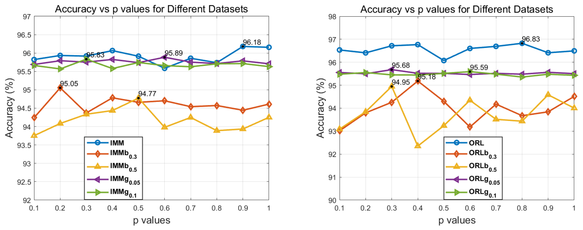
Selecting an appropriate p for unseen datasets depends on the expected noise characteristics, driven by the theoretical properties of the ${\mathsf{\ell }}_p$-norm. The derivative of the ${\mathsf{\ell }}_p$ penalty with respect to a residual e is proportional to ${\left|e\right|}^{p-1}$. While a smaller p increases robustness against outliers, it also exacerbates the non-convexity of the objective function. Therefore, the choice of p is a trade-off between robustness and optimization stability.

Figure 1 illustrates this trade-off by plotting the clustering accuracy of R2DDC against p on the IMM and ORL datasets. The empirical trends align with the theoretical analysis and can be categorized into three scenarios:

• Gross Corruptions (e.g., Block Occlusion): Severe, sparse outliers require a smaller p to suppress large errors. As shown in Figure 1, accuracy peaks sharply within $p\in [0.3,0.5]$ and degrades for larger values.
• Dense/Uniform Noise (e.g., Gaussian Noise): For dense, moderate noise, the model requires a balance between noise suppression and stability. The performance curves remain relatively flat, with optimums generally observed at moderate values ($p\in [0.3,0.6]$).
• Clean Data: Without outliers, a small p introduces unnecessary non-convexity. Larger values ($p\in [0.8,1.0]$) yield a smoother optimization landscape, with accuracy typically maximizing near $p=1.0$.

Practical Recommendation: For new datasets, we recommend setting $p\in [0.3,0.5]$ if structural occlusions or severe sensor errors are anticipated. For data with standard natural noise, $p\in [0.4,0.6]$ serves as a stable default. For strictly clean data, $p\in [0.8,1.0]$ is preferred.

5. Conclusions

A robust ${\mathsf{\ell }}_p$-norm two-dimensional discriminative clustering (R2DDC) method was presented in this paper. By adopting the ${\mathsf{\ell }}_p$ norm, R2DDC enhances robustness against outliers and noise. The method jointly considers discriminative and structural information, enabling dimensionality reduction and clustering to be performed in a unified framework. Experimental results on several face image datasets show that the proposed approach achieves competitive performance. Future work could extend the method to multi-view data and develop nonlinear variants via kernel methods or deep learning. The source code and datasets required to reproduce all findings in this study are publicly available at: https://github.com/YangSkywalker/R2DDC (accessed on 10 July 2026).

References

1. Wang, K.; Wang, L.; Zhang, X.; Li, J. Continual Multiview Spectral Clustering via Multilevel Knowledge. IEEE Signal Process. Lett. 2024, 31, 1555–1559. [Google Scholar] [CrossRef] [Scilit]
2. Meng, B.; Li, F.; Yang, F.; Gao, Q. Centroid-Free K-Means With Balanced Clustering. IEEE Signal Process. Lett. 2025, 32, 1191–1195. [Google Scholar] [CrossRef] [Scilit]
3. Singh, V.; Verma, N.K. Gene Expression Data Analysis Using Feature Weighted Robust Fuzzy K-Means Clustering. IEEE Trans. NanoBiosci. 2023, 22, 99–105. [Google Scholar] [CrossRef] [Scilit]
4. Maheshwari, R.; Mishra, A.C.; Mohanty, S.K. An entropy based density peak clustering for numerical gene expression datasets. Appl. Soft Comput. 2023, 142, 110321. [Google Scholar] [CrossRef] [Scilit]
5. Abualigah, L.; Almotairi, K.H.; Al-qaness, M.A.; Ewees, A.A.; Yousri, D.; Abd Elaziz, M.; Nadimi-Shahraki, M.H. Efficient text document clustering approach using multi-search arithmetic optimization algorithm. Knowl. Based Syst. 2022, 248, 108833. [Google Scholar] [CrossRef] [Scilit]
6. Zhang, H.; Li, H.; Chen, N.; Chen, S.; Liu, J. Novel fuzzy clustering algorithm with variable multi-pixel fitting spatial information for image segmentation. Pattern Recognit. 2022, 121, 108201. [Google Scholar] [CrossRef] [Scilit]
7. Fang, U.; Li, J.X.; Lu, X.Q.; Gao, L.X.; Ali, M.; Xiang, Y. Self-supervised cross-iterative clustering for unlabeled plant disease images. Neurocomputing 2021, 456, 36–48. [Google Scholar] [CrossRef] [Scilit]
8. Ikotun, A.M.; Ezugwu, A.E.; Abualigah, L.; Abuhaija, B.; Heming, J. k-means clustering algorithms: A comprehensive review, variants analysis, and advances in the era of big data. Inf. Sci. 2023, 622, 178–210. [Google Scholar] [CrossRef] [Scilit]
9. Bradley, P.S.; Mangasarian, O.L. k-plane clustering. J. Glob. Optim. 2000, 16, 23–32. [Google Scholar] [CrossRef] [Scilit]
10. Tseng, P. Nearest q-Flat to m Points. J. Optim. Theory Appl. 2000, 105, 249–252. [Google Scholar] [CrossRef] [Scilit]
11. Liu, L.M.; Guo, Y.R.; Wang, Z.; Yang, Z.M.; Shao, Y.H. k-proximal plane clustering. Int. J. Mach. Learn. Cybern. 2017, 8, 1537–1554. [Google Scholar] [CrossRef] [Scilit]
12. Yang, Z.M.; Guo, Y.R.; Li, C.N.; Shao, Y.H. Local k-proximal plane clustering. Neural Comput. Appl. 2015, 26, 199–211. [Google Scholar] [CrossRef] [Scilit]
13. Wang, J.; Liu, Y.; Fu, L. Robust local k-proximal plane clustering based on l2,1-norm minimization. Int. J. Mach. Learn. Cybern. 2024, 15, 5143–5158. [Google Scholar] [CrossRef] [Scilit]
14. Wang, Z.; Shao, Y.H.; Bai, L.; Deng, N.Y. Twin Support Vector Machine for Clustering. IEEE Trans. Neural Netw. Learn. Syst. 2015, 26, 2583–2588. [Google Scholar] [CrossRef] [Scilit]
15. Bai, L.; Shao, Y.H.; Wang, Z.; Li, C.N. Clustering by twin support vector machine and least square twin support vector classifier with uniform output coding. Knowl. Based Syst. 2019, 163, 227–240. [Google Scholar] [CrossRef] [Scilit]
16. Tanveer, M.; Gupta, T.; Shah, M.; Richhariya, B. Sparse Twin Support Vector Clustering Using Pinball Loss. IEEE J. Biomed. Health Inform. 2021, 25, 3776–3783. [Google Scholar] [CrossRef] [Scilit]
17. Zhu, J.; Chen, S.; Liu, Y.; Hu, C. Energy-based structural least squares twin support vector clustering. Eng. Appl. Artif. Intell. 2024, 128, 107467. [Google Scholar] [CrossRef] [Scilit]
18. Li, C.N.; Shao, Y.H.; Guo, Y.R.; Wang, Z.; Yang, Z.M. Robust k-subspace discriminant clustering. Appl. Soft Comput. 2019, 85, 105858. [Google Scholar] [CrossRef] [Scilit]
19. Qi, Y.F.; Shao, Y.H.; Li, C.N.; Guo, Y.R. Locally finite distance clustering with discriminative information. Inf. Sci. 2023, 623, 607–632. [Google Scholar] [CrossRef] [Scilit]
20. Guo, Y.R.; Bai, Y.Q. Two-dimensional k-subspace clustering and its applications on image recognition. Int. J. Mach. Learn. Cybern. 2023, 14, 2671–2683. [Google Scholar] [CrossRef] [Scilit]
21. Li, Z.; Yao, L.; Wang, S.; Kanhere, S.; Li, X.; Zhang, H. Adaptive two-dimensional embedded image clustering. In Proceedings of the AAAI Conference on Artificial Intelligence, New York, NY, USA, 7–12 February 2020; pp. 4796–4803. [Google Scholar] [CrossRef] [Scilit]
22. Guo, Y.R.; Guo, T.T.; Li, C.N.; Hua, X.Y. Capped l2,1-norm two-dimensional k-subspace clustering. Clust. Comput. 2026, 29, 277. [Google Scholar] [CrossRef] [Scilit]
23. Li, C.N.; Shao, Y.H.; Wang, Z.; Deng, N.Y. Robust bilateral Lp-norm two-dimensional linear discriminant analysis. Inf. Sci. 2019, 500, 274–297. [Google Scholar] [CrossRef] [Scilit]
24. Zheng, W.; Lin, Z.; Wang, H. L1-Norm Kernel Discriminant Analysis Via Bayes Error Bound Optimization for Robust Feature Extraction. IEEE Trans. Neural Netw. Learn. Syst. 2014, 25, 793–805. [Google Scholar] [CrossRef] [Scilit]
25. Yu, M.; Shao, L.; Zhen, X.; He, X. Local Feature Discriminant Projection. IEEE Trans. Pattern Anal. Mach. Intell. 2016, 38, 1908–1914. [Google Scholar] [CrossRef] [Scilit]
26. Sun, B.; Zhou, P.; Du, L.; Li, X. Active deep image clustering. Knowl. Based Syst. 2022, 252, 109346. [Google Scholar] [CrossRef] [Scilit]
27. Wu, S.; Zheng, Y.; Ren, Y. Self-weighted contrastive fusion for deep multi-view clustering. IEEE Trans. Multimed. 2024, 26, 9150–9162. [Google Scholar] [CrossRef] [Scilit]
28. Ros, F.; Riad, R.; Guillaume, S. Deep clustering framework review using multicriteria evaluation. Knowl. Based Syst. 2024, 285, 111315. [Google Scholar] [CrossRef] [Scilit]
29. Nordstrøm, M.; Larsen, M.; Sierakowski, J.; Stegmann, M.B. The IMM Face Database—An Annotated Dataset of 240 Face Images. Technical University of Denmark. 2004. Available online: https://www2.imm.dtu.dk/pubdb/pubs/3160-full.html (accessed on 10 July 2026).
30. AT&T Laboratories Cambridge. The ORL Database of Faces. AT&T Laboratories Cambridge. 1994. Available online: https://www.cl.cam.ac.uk/research/dtg/attarchive/facedatabase.html (accessed on 10 July 2026).
31. Belhumeur, P.N.; Hespanha, J.P.; Kriegman, D.J. Eigenfaces vs. Fisherfaces: Recognition using class specific linear projection. IEEE Trans. Pattern Anal. Mach. Intell. 1997, 19, 711–720. [Google Scholar] [CrossRef] [Scilit]
32. Martinez, A.M.; Benavente, R. The AR Face Database; CVC Technical Report #24; Computer Vision Center: Barcelona, Spain, 1998. [Google Scholar]
33. Phillips, P.J.; Moon, H.; Rizvi, S.A.; Rauss, P.J. The FERET evaluation methodology for face-recognition algorithms. IEEE Trans. Pattern Anal. Mach. Intell. 2000, 22, 1090–1104. [Google Scholar] [CrossRef] [Scilit]
Figure 1. Accuracy (%) versus p on the IMM (left) and ORL (right) datasets under clean, block-occlusion, and Gaussian-noise conditions.
Applsci 16 08883 g001