Cascaded Acceleration–Velocity Control of a PMDC Motor for Flywheel Energy Storage Systems with Planetary Transmission

Abstract

Flywheel energy storage systems coupled with planetary transmissions require accurate carrier motion control to support efficient energy exchange and operation with carrier torque close to zero. This paper develops a digital cascaded acceleration and velocity control framework for a permanent magnet DC motor used as the carrier actuator in a planetary-transmission flywheel energy storage system. The controller combines an outer velocity loop, an inner acceleration loop, and a feedforward angular acceleration reference derived from the desired motion profile. Two digital implementation approaches are examined. The first preserves the continuous motor plant and includes A/D conversion, aliasing prevention and D/A reconstruction effects. The second uses a fully discrete acceleration plant for adaptive controller design. Based on this discrete model, two adaptive inner acceleration controllers are developed: adaptive deadbeat control and adaptive pole placement control. Both controllers replace only the inner acceleration PI controller, while the outer velocity loop and the feedforward structure remain unchanged. A normalized gradient estimator with projection updates the discrete plant coefficients online and keeps the estimates within calculated admissible bounds. Scilab/Xcos simulations evaluate the controllers under pulse acceleration disturbance, sinusoidal acceleration disturbance, and segmented reference tracking. The results show that both adaptive controllers reduce angular acceleration and angular velocity tracking errors compared with the digital PI baseline. The adaptive deadbeat controller gives the fastest response, whereas the adaptive pole placement controller provides a tunable compromise between response speed and smoothness.

1. Introduction

Flywheel energy storage systems (FESSs) are attractive for applications that require high power density, rapid charge and discharge operation, long cycle life, and repeated regenerative energy exchange. In railway and vehicle applications, a flywheel can absorb kinetic energy during braking and return it during acceleration, thereby reducing energy losses and improving system efficiency. Jackiewicz introduced a flywheel based regenerative braking concept in which a planetary transmission regulates the energy exchange between the drivetrain and the flywheel [1,2]. In that configuration, the carrier motion plays a central role. The carrier torque should remain close to zero, while the carrier velocity should follow a linear profile. This operating condition requires accurate regulation of both angular velocity and angular acceleration. Therefore, the motor connected to the planetary carrier should not be treated only as a conventional speed actuator. Its acceleration dynamics must also be included in the controller design.

Recent studies confirm that flywheel energy storage remains an active research area for transportation, renewable energy systems, and grid support applications. Reviews of FESS technologies emphasize their suitability for high power operation, regenerative braking, load frequency regulation, and applications that require frequent cycling [3,4,5,6]. In railway and urban transit systems, the recovery of braking energy is especially important because braking and acceleration occur repeatedly over short operating intervals. Researchers have studied wayside and onboard storage systems to improve energy use in DC railway networks and metro systems [7,8,9,10]. Hybrid propulsion concepts for rail vehicles also show that energy storage and power management strategies can significantly influence system level performance [11]. These studies demonstrate the relevance of FESS technology and show that effective control of the electromechanical interface is essential for practical implementation.

A planetary transmission introduces additional control requirements because the rotational speeds and torques of the sun gear, ring gear, and carrier are mechanically coupled. Planetary gear trains are widely used when compactness, torque distribution, and multiple speed paths are required [12]. Similar mechanical coupling principles also appear in electric and hybrid vehicle powertrains, especially in power split and continuously variable transmission concepts [13,14]. However, the flywheel transmission considered here actively controls the carrier using a permanent magnet DC motor (PMDC motor), and the desired operating condition requires controlled acceleration and carrier torque close to zero. This requirement differs from conventional motor speed regulation because the controller must generate a prescribed angular velocity trajectory while maintaining the corresponding acceleration profile. The problem also relates to railway longitudinal dynamics, where acceleration limits, velocity profiles, and traction or braking transitions directly affect system behavior and passenger comfort [15,16,17,18]. Previous studies on train longitudinal dynamics and coupler force reduction further show that accurate dynamic modeling and control can improve the behavior of multibody railway systems [19,20].

Conventional PMDC motor control is commonly formulated as a speed control problem, where a proportional integral or proportional integral derivative controller reduces the angular velocity tracking error. Classical and modern control references provide the fundamental basis for motor modeling, feedback control, stability analysis, discrete time pole assignment, and digital controller implementation [21,22,23,24,25]. However, a single velocity loop is not sufficient for the present application because the acceleration must also follow a prescribed profile. A cascaded control structure is more suitable for this purpose. In this structure, the outer loop regulates the slower or higher level variable, while the inner loop regulates a faster variable that relates more directly to the actuator dynamics. For the PMDC carrier actuator, the outer loop regulates velocity, while the inner loop regulates acceleration. This arrangement allows the controller to handle the desired angular velocity trajectory and its associated acceleration command consistently.

Digital implementation is also essential because a practical test bench controller will operate on a microprocessor or real time control platform. Digital control requires attention to sampling, discretization, computation delay, aliasing prevention, and signal reconstruction. The later stability evaluation also relies on discrete characteristic root locations and Jury type stability conditions, which are commonly used for discrete time systems and numerical stability assessment [25,26]. These topics are well established in sampled data and digital control theory [23,27,28]. Two digital implementation approaches are considered in this paper. The first preserves the continuous motor plant and introduces digital conversion effects, including A/D conversion, aliasing prevention and D/A reconstruction. This approach is close to the physical test bench situation, where the motor remains a continuous electromechanical plant but the controller operates digitally. The second approach converts the PMDC acceleration dynamics into a fully discrete state space model, which supports adaptive inner loop control because the controller uses the discrete acceleration plant coefficients directly.

Adaptive control is useful when plant parameters are uncertain, variable, or affected by unmodeled dynamics. Standard adaptive control methods use online parameter estimation and controller adjustment to improve performance under model uncertainty [29,30,31,32]. Adaptive laws often include projection or bounding mechanisms to keep online parameter estimates inside prescribed admissible sets, especially when the estimated coefficients are used directly in model based control laws [33]. Recent studies have continued to develop parameter estimation and adaptive control methods for dynamic systems, including improved estimator formulations and adaptive motor control strategies [34,35]. For motor drives, adaptive and model based control can improve transient response and robustness compared with fixed gain controllers, especially when the system operates under changing load or disturbance conditions. Deadbeat and pole placement methods are particularly relevant for discrete time systems because they use the plant model to assign the closed loop response directly. Recent motor control studies have applied deadbeat predictive and pole placement based adaptive methods to improve current, speed, and dynamic response characteristics [36,37]. Researchers have also investigated cascade based motor control structures to improve speed regulation and disturbance response [38].

Despite these developments, the control problem addressed in this paper remains insufficiently developed in the available literature. Existing FESS studies mainly focus on energy storage technologies, railway energy recovery, power management, or system-level storage performance [4,5,6,39]. These works usually do not examine the acceleration control of the motor that regulates the carrier motion in a planetary-transmission flywheel system. At the same time, motor control studies commonly focus on speed, current, or torque regulation. However, the present application requires the carrier velocity to follow a prescribed trajectory while its acceleration is also explicitly controlled. This requirement is directly related to the low carrier torque of the planetary gearset, which results solely from the coupling effect of friction and the mass moment of inertia of the planetary gear mechanism reduced to the carrier axis [40,41]. This favors low-loss bidirectional energy exchange in the flywheel system [1,2].

The novelty of this work is therefore not only the use of adaptive control for a PMDC motor, but its application to the inner acceleration loop of a cascaded carrier-motion controller for a planetary-transmission FESS. The proposed formulation treats the PMDC motor as a discrete acceleration plant. Based on this model, the fixed inner acceleration PI controller is replaced with adaptive deadbeat and adaptive pole-placement controllers. This gives a direct model-based link between the commanded acceleration and the voltage command, while the outer velocity loop and the feedforward acceleration reference remain unchanged. In this way, the paper connects the mechanical requirement of the flywheel transmission with a digital adaptive acceleration-control structure suitable for future test-bench implementation.

In this paper, we intend to popularize a more cost-effective solution. This approach serves as an alternative to both the digital cascade speed control of permanent-magnet DC motors proposed by Gondhalekar [42] and the field-oriented control of permanent-magnet motors. It should be emphasized that, to date, the cascade control of Gondhalekar’s DC brushed motor is the only known commercially available solution. Moreover, we intend to create a suitable control system for an electronic continuously variable transmission (e-CVT) that could achieve high mechanical efficiency, in the range of 95–97%, similar to the groundbreaking gear-based continuously variable transmission “Ratio Zero”, but without its drawbacks. These disadvantages include a high degree of mechanical complexity and the risk of vibration resulting from speed pulsations.

The main contributions of this paper are as follows:

• A digital cascaded acceleration and velocity control architecture is developed for a PMDC carrier actuator in a planetary-transmission flywheel energy storage system.
• The PMDC motor is reformulated as an acceleration plant whose input is the discrete voltage derivative and whose output is angular acceleration.
• Two digital implementation approaches are presented: a sampled-data realization with converter effects and a fully discrete state-space realization for adaptive controller design.
• Two adaptive inner-loop acceleration controllers are developed using a normalized gradient parameter estimator with projection.
• The proposed adaptive controllers are compared with the baseline digital PI controller under pulse disturbance, sinusoidal disturbance, and segmented reference-tracking conditions.

2. System Modeling and Digital Cascaded Control Architecture

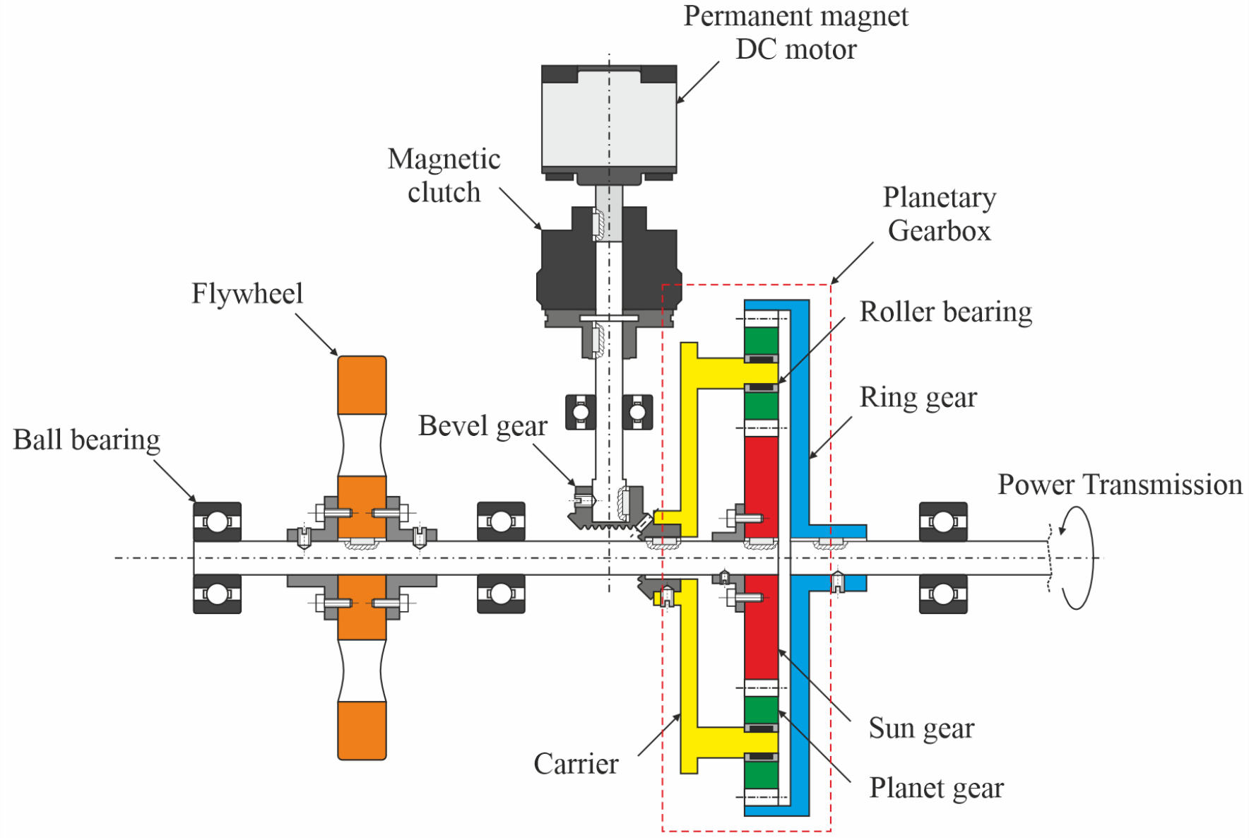
The proposed controller is developed for a PMDC motor connected to the carrier of a planetary transmission in a flywheel energy storage system. Figure 1 shows the mechanical arrangement considered in this work. The system consists of a permanent magnet DC motor, a magnetic clutch, a bevel gear stage, a planetary gearbox, a flywheel, and the mechanical connection to the vehicle power transmission. The PMDC motor connects to the planetary carrier through the magnetic clutch and bevel gear stage, while the flywheel connects mechanically to the sun gear. The external ring gear connects to the vehicle power transmission path and provides the mechanical interface with the train wheels.

During regenerative braking, kinetic energy from the vehicle wheels passes through the powertrain and ring gear into the planetary gearbox, and then transfers to the flywheel through the sun gear path. During vehicle acceleration, the energy flow reverses, and the flywheel returns the stored energy through the planetary transmission to the driven wheels. The controlled carrier motion adjusts the kinematic relationship among the ring gear, sun gear, and flywheel. This motion supports efficient bidirectional energy exchange and the carrier torque condition close to zero described in the original flywheel transmission concept [1].

The magnetic clutch provides a practical means of engaging or disengaging the PMDC motor from the carrier drive during startup, shutdown, protection procedures, and experimental test bench operation. The present control model assumes that the clutch remains fully engaged during controlled operation. Transient clutch engagement dynamics are therefore outside the scope of the present model.

The mechanical transmission model used in this study is therefore treated as an idealized kinematic interface for the purpose of controller development. Transmission efficiency losses, bearing friction, gear backlash, shaft compliance, clutch slip, and other nonlinear mechanical effects are not modeled explicitly in the present numerical study. These effects can influence the carrier torque, introduce additional delay or hysteresis, and modify the actual acceleration response of the physical system. In the present work, their influence is considered indirectly through acceleration-level disturbances and through the discussion of implementation limitations. A detailed electromechanical model including friction, backlash, transmission losses, and clutch engagement dynamics will be required for the next experimental stage of the planetary-transmission flywheel test bench.

For a planetary gear system operating under unsteady conditions, the fundamental torque balance can be formulated using D’Alembert’s principle by considering the external moments, internal meshing forces, and inertial reactions. In the considered operating mode, the angular accelerations of the ring and sun gear act with opposite signs. Therefore, the inertia-related effects can be reduced through a suitable optimization of the planetary gear geometry and the corresponding equivalent inertia referred to the carrier axis [40,41]. This observation supports the simplified model used in the present controller-design stage, while a more detailed nonlinear drivetrain model is left for the experimental validation stage.

2.1. PMDC Motor Model

The PMDC motor is modeled using the standard armature controlled motor equation. Neglecting the armature inductance, the transfer function from motor voltage $V\left(t\right)$ to angular velocity $\omega \left(t\right)$ is

$${\displaystyle \frac{\mathsf{\Omega }\left(s\right)}{V\left(s\right)}}={\displaystyle \frac{K_m}{J_{eq}{R}_{m}s+K_m^2}}$$

(1)

where $K_m$ is the motor constant, $R_m$ is the armature resistance, and $J_{eq}$ is the equivalent inertia referred to the motor shaft. This first order model is commonly used for PMDC motor control when the electrical time constant is small relative to the mechanical dynamics [21,22].

Equation (1) can be rewritten in time domain form as

$$\dot{\omega }\left(t\right)=-a\omega \left(t\right)+bV\left(t\right)$$

(2)

where

$$a={\displaystyle \frac{K_m^2}{J_{eq}{R}_m}},b={\displaystyle \frac{K_m}{J_{eq}{R}_m}}.$$

(3)

The angular acceleration is defined as $\epsilon \left(t\right)=\dot{\omega }\left(t\right)$. Differentiating Equation (2) gives the acceleration plant representation

$$\dot{\epsilon }\left(t\right)=-a\epsilon \left(t\right)+b\dot{V}\left(t\right).$$

(4)

Thus, the PMDC motor can be represented as an acceleration plant whose input is the voltage derivative $\dot{V}\left(t\right)$ and whose output is the angular acceleration $\epsilon \left(t\right)$. This representation is important because the proposed controller uses an inner acceleration loop rather than relying only on a conventional speed control loop. The continuous time state space representation of the acceleration subsystem is

$$\begin{array}{cc}\hfill \dot{x}\left(t\right)& =Ax\left(t\right)+Bu\left(t\right),\hfill \\ \hfill y\left(t\right)& =Cx\left(t\right)+Du\left(t\right)\hfill \end{array}$$

(5)

with

$$x\left(t\right)=\epsilon \left(t\right),u\left(t\right)=\dot{V}\left(t\right),A=-a,B=b,C=1,D=0.$$

(6)

The acceleration plant in Equation (4) should be interpreted as a control-oriented representation of the PMDC carrier actuator. It does not introduce a new physical input to the motor; the physical actuator input remains the motor voltage $V\left(t\right)$. The term $\dot{V}\left(t\right)$ appears because the velocity model is differentiated to express the acceleration dynamics directly. This formulation is useful for the proposed cascaded structure, where the inner loop controls angular acceleration and the outer loop controls angular velocity.

In the digital implementation, the plant input is therefore represented by the discrete voltage derivative $u\left[k\right]$, which is generated from the voltage command through a filtered derivative. This filtering is necessary because direct numerical differentiation can amplify measurement noise and high-frequency components. Consequently, the acceleration-plant model is suitable for controller design and numerical evaluation, but its practical implementation requires careful filtering, sampling-time selection, and delay assessment before application to the physical test bench.

2.2. Discrete Formulation of the Acceleration Loop Components

For the fully discrete implementation, the continuous acceleration subsystem in Equation (4) is discretized with the sampling period $T_s$. The resulting discrete state space model is written as

$$\begin{array}{cc}\hfill x[k+1]& =A_{d}x\left[k\right]+B_{d}u\left[k\right],\hfill \\ \hfill y\left[k\right]& =C_{d}x\left[k\right]+D_{d}u\left[k\right]\hfill \end{array}$$

(7)

where

$$x\left[k\right]=\epsilon \left[k\right],x[k+1]=\epsilon [k+1],u\left[k\right]=\dot{V}\left[k\right],y\left[k\right]=\epsilon \left[k\right].$$

(8)

Thus, the discrete acceleration model becomes

$$\epsilon [k+1]=A_d\epsilon \left[k\right]+B_{d}u\left[k\right].$$

(9)

The discrete coefficients are

$$A_d=e^{-a{T}_s},B_d={\displaystyle \frac{b}{a}}\left(1-e^{-a{T}_s}\right),C_d=1,D_d=0.$$

(10)

Taking the z-transform of Equation (9), the corresponding discrete transfer function from $U\left(z\right)$ to $E\left(z\right)$ is

$$G_{\epsilon }\left(z\right)={\displaystyle \frac{E\left(z\right)}{U\left(z\right)}}={\displaystyle \frac{C_d{B}_d}{z-A_d}}+D_d={\displaystyle \frac{B_d}{z-A_d}}.$$

(11)

The digital PI controllers are implemented using the Tustin approximation, a standard bilinear transformation method in digital control design [23,27]. For a continuous PI controller

$$C\left(s\right)=K_p+{\displaystyle \frac{K_i}{s}},$$

(12)

the Tustin approximation gives the incremental digital PI form

$$c\left[k\right]=c[k-1]+q_{0}e\left[k\right]+q_{1}e[k-1]$$

(13)

where $e\left[k\right]$ is the controller input error, $c\left[k\right]$ is the controller output, and

$$q_0=K_p+{\displaystyle \frac{K_i{T}_s}{2}},q_1=-K_p+{\displaystyle \frac{K_i{T}_s}{2}}.$$

(14)

For the inner acceleration controller, the error input is $e_{\epsilon }\left[k\right]$ and the controller output is the voltage command $V\left[k\right]$. Therefore, the acceleration PI controller transfer function is

$$C_{\epsilon }\left(z\right)={\displaystyle \frac{V\left(z\right)}{E_{\epsilon }\left(z\right)}}={\displaystyle \frac{q_{0\epsilon }z+q_{1\epsilon }}{z-1}}$$

(15)

where coefficients $q_{0\epsilon }$ and $q_{1\epsilon }$ are obtained from Equation (14) by using $K_p=K_{p\epsilon }$ and $K_i=K_{i\epsilon }$.

In the baseline digital PI implementation, the voltage derivative is generated using a filtered discrete derivative. The recursive form is

$$u\left[k\right]={\alpha }_{d}u[k-1]+{\beta }_d\left(V\left[k\right]-V[k-1]\right)$$

(16)

where

$${\alpha }_d={\displaystyle \frac{T_f}{T_f+T_s}},{\beta }_d={\displaystyle \frac{1}{T_f+T_s}}.$$

(17)

The corresponding transfer function from the voltage command to the discrete plant input is

$$D_V\left(z\right)={\displaystyle \frac{U\left(z\right)}{V\left(z\right)}}={\displaystyle \frac{{\beta }_d(z-1)}{z-{\alpha }_d}}.$$

(18)

2.3. Conceptual Cascaded Acceleration and Velocity Control Architecture

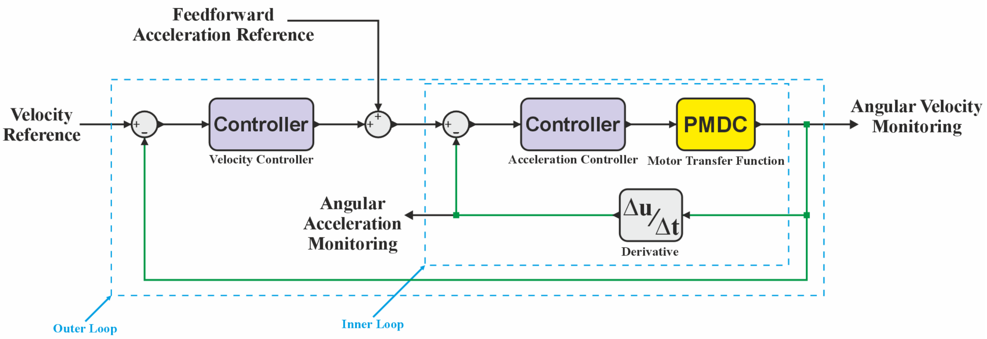
The proposed controller uses a cascaded architecture with an outer velocity loop and an inner acceleration loop. The outer loop regulates angular velocity tracking, while the inner loop regulates the angular acceleration response of the PMDC motor. Acceleration feedback is appropriate for the carrier control problem because the desired operating condition requires both a prescribed angular velocity trajectory and controlled acceleration or deceleration.

The velocity tracking error, feedforward acceleration summation, and acceleration tracking error are defined as

$$e_{\omega }\left[k\right]={\omega }_{ref}\left[k\right]-\omega \left[k\right],{\epsilon }_c\left[k\right]={\epsilon }_{ref}\left[k\right]+u_{\omega }\left[k\right],e_{\epsilon }\left[k\right]={\epsilon }_c\left[k\right]-\epsilon \left[k\right].$$

(19)

Here, ${\omega }_{ref}\left[k\right]$ is the velocity reference, $\omega \left[k\right]$ is the measured velocity, $u_{\omega }\left[k\right]$ is the velocity controller output, ${\epsilon }_{ref}\left[k\right]$ is the feedforward acceleration reference, and ${\epsilon }_c\left[k\right]$ is the commanded acceleration for the inner loop. The feedforward acceleration reference provides the acceleration demand associated with the intended velocity trajectory, while the outer velocity loop corrects accumulated tracking error. This arrangement separates trajectory regulation from acceleration tracking. The conceptual signal flow of the cascaded structure is presented in Figure 2.

2.4. Digital Implementation Structures

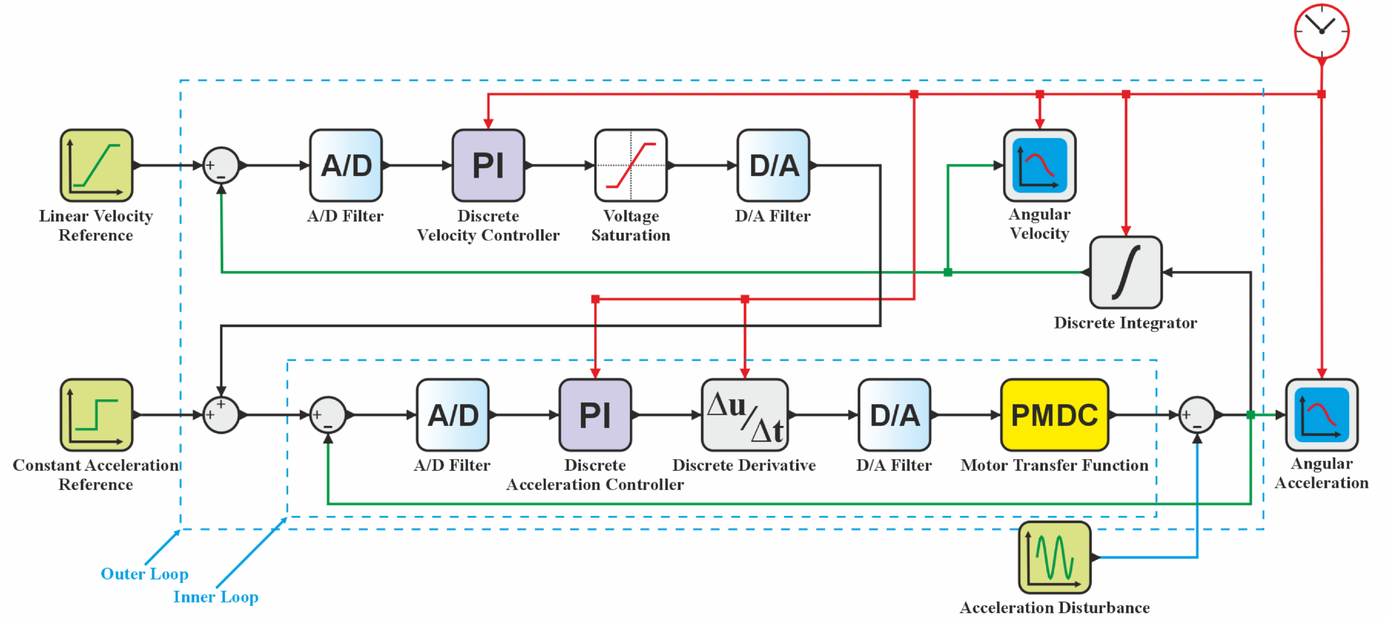
The first digital implementation approach preserves the continuous PMDC motor transfer function and introduces converter effects around the digital control blocks. Following the sampled data representation described by Thomas [28], the anti aliasing filter associated with A/D conversion is represented as

$$G_{AD}\left(s\right)={\displaystyle \frac{{(1/T_s)}^2}{{(s+0.707/T_s)}^2+{(0.707/T_s)}^2}}$$

(20)

and the D/A converter is represented as

$$G_{DA}\left(s\right)={\displaystyle \frac{2/T_s}{s+2/T_s}}.$$

(21)

This representation allows implementation effects to be evaluated before moving to a physical test bench, because the controller operates digitally while the motor remains a continuous electromechanical plant. The sampled data realization in Figure 3 includes the main conversion and reconstruction effects considered in this work.

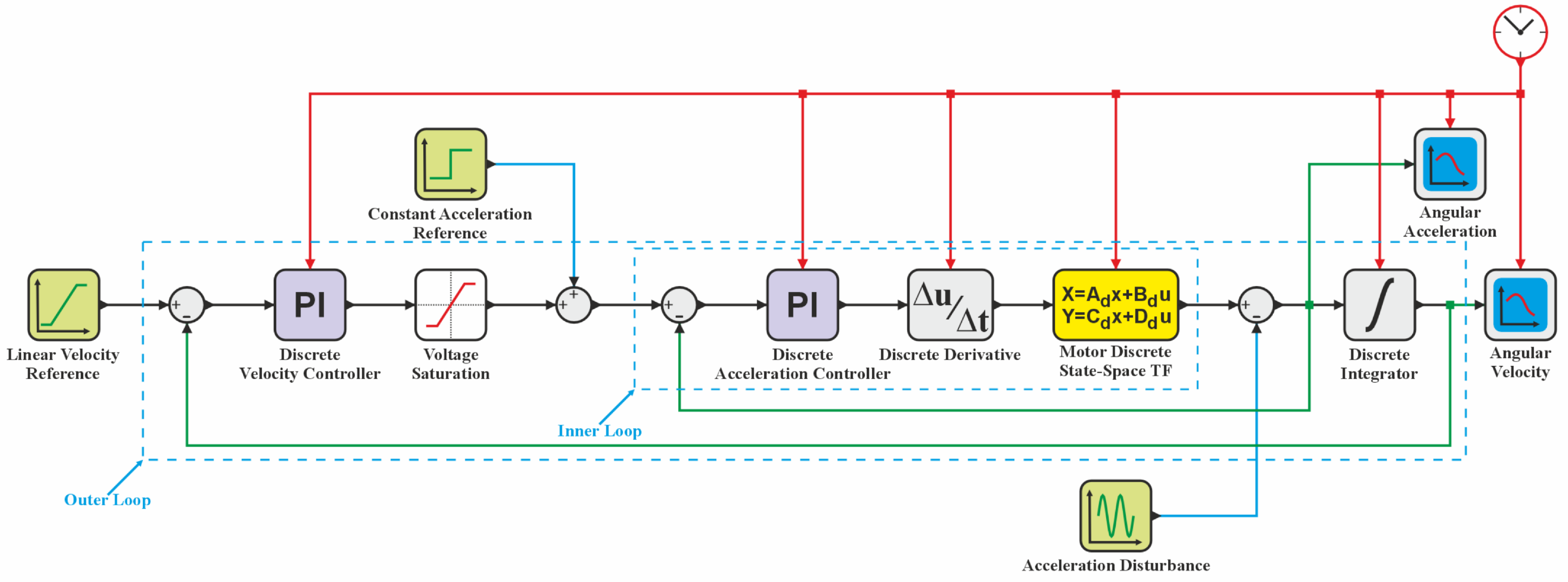
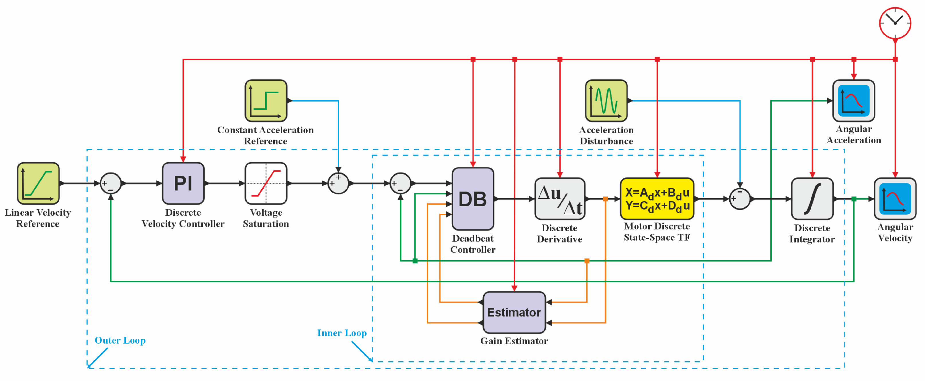
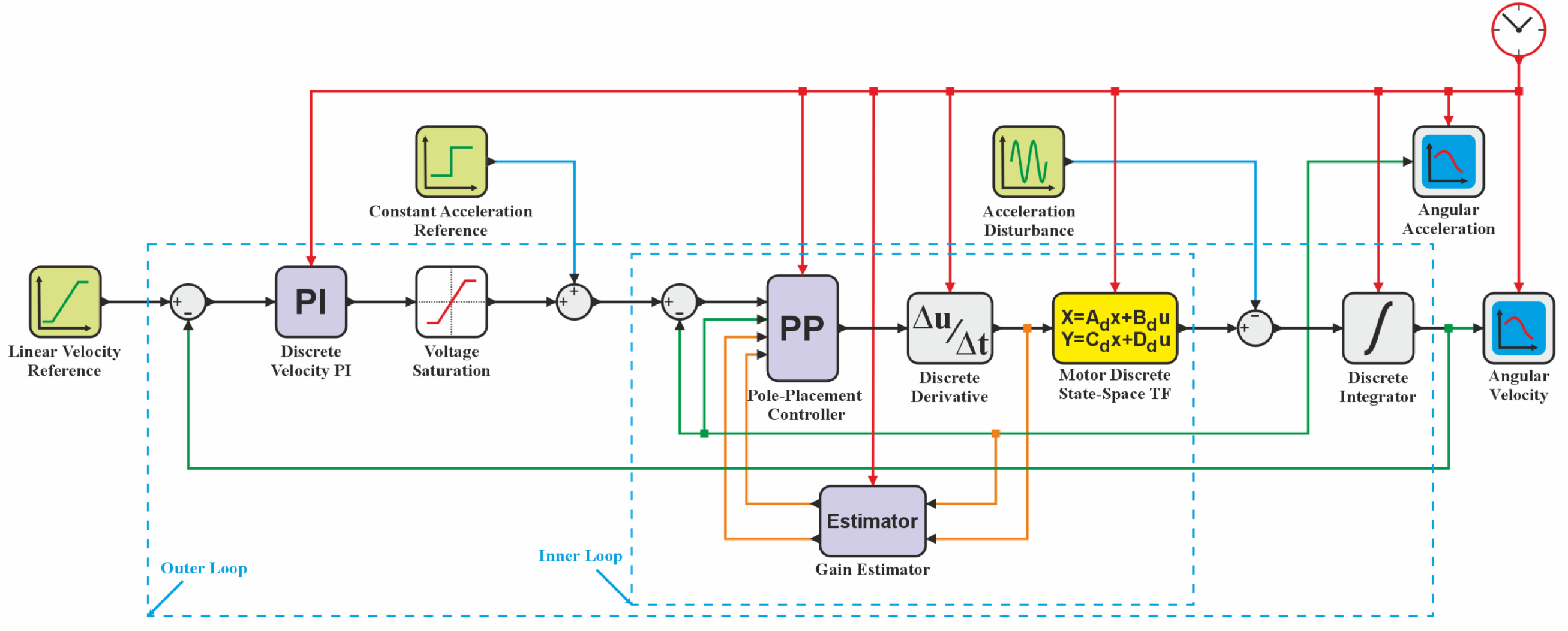
The second digital implementation employs the fully discrete acceleration plant in Equation (9). The voltage command $V\left[k\right]$ is related to the plant input $u\left[k\right]$ through the filtered derivative relation in Equation (16), while the PMDC motor acceleration dynamics are implemented by the discrete state-space block. The velocity signal is then reconstructed from the acceleration response using the discrete integrator

$$\omega \left[k\right]=\omega [k-1]+T_s\epsilon \left[k\right].$$

(22)

This fully discrete representation forms the basis for the digital control structures investigated in the following sections, as illustrated in Figure 4.

2.5. Nominal Baseline Inner Acceleration Loop Stability Analysis

The stability of the baseline inner acceleration loop must be evaluated from the closed loop transfer function of the nominal PI based loop. The discrete acceleration plant alone does not represent the complete baseline loop, because this loop also includes the acceleration PI controller and the filtered discrete derivative block.

Using Equations (11), (15) and (18), the nominal inner loop is obtained as the cascade $C_{\epsilon }\left(z\right)D_V\left(z\right)G_{\epsilon }\left(z\right)$. The derivative block maps the voltage command $V\left(z\right)$ to the plant input $U\left(z\right)$, and the factor $(z-1)$ in $D_V\left(z\right)$ cancels the corresponding factor in the PI controller denominator. Therefore, the nominal open loop transfer function becomes

$$L_{\epsilon }\left(z\right)=C_{\epsilon }\left(z\right)D_V\left(z\right)G_{\epsilon }\left(z\right)={\displaystyle \frac{{\beta }_d{B}_d(q_{0\epsilon }z+q_{1\epsilon })}{(z-{\alpha }_d)(z-A_d)}}.$$

(23)

The corresponding closed loop transfer function from the commanded acceleration $E_c\left(z\right)$ to the acceleration response $E\left(z\right)$ is

$$T_{\epsilon }\left(z\right)={\displaystyle \frac{E\left(z\right)}{E_c\left(z\right)}}={\displaystyle \frac{{\beta }_d{B}_d(q_{0\epsilon }z+q_{1\epsilon })}{(z-{\alpha }_d)(z-A_d)+{\beta }_d{B}_d(q_{0\epsilon }z+q_{1\epsilon })}}.$$

(24)

The characteristic polynomial of the nominal inner acceleration loop is

$$P_{\epsilon }\left(z\right)=z^2+a_{1}z+a_0$$

(25)

where

$$a_1=-({\alpha }_d+A_d)+{\beta }_d{B}_d{q}_{0\epsilon },a_0={\alpha }_d{A}_d+{\beta }_d{B}_d{q}_{1\epsilon }.$$

(26)

For a second order discrete time polynomial $z^2+a_{1}z+a_0$, the Jury stability conditions are [25,26]

$$1+a_1+a_0>0,1-a_1+a_0>0,1-a_0>0.$$

(27)

Equivalently, the two closed loop poles are obtained from

$$z_{1,2}={\displaystyle \frac{-a_1\pm \sqrt{a_1^2-4a_0}}{2}}$$

(28)

and must satisfy

$$|z_1|<1,|z_2|<1.$$

(29)

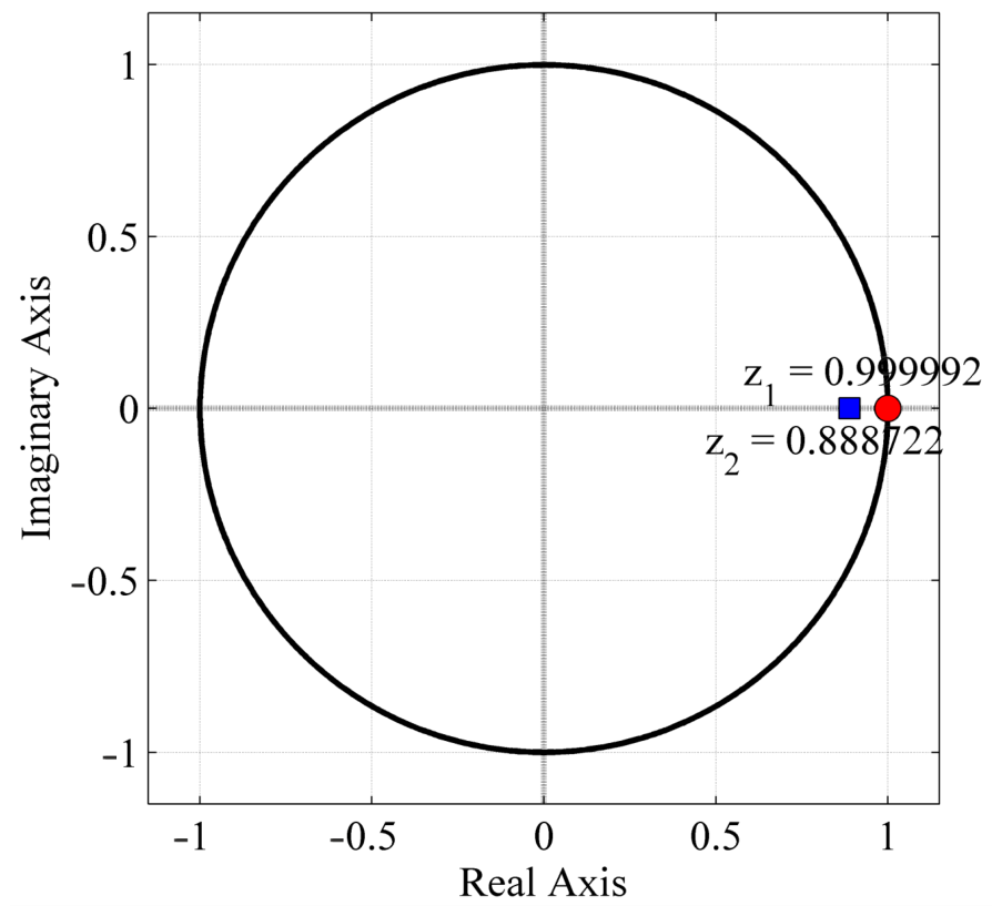
Using the nominal motor parameters $K_m=0.028$ V s/rad, $R_m=3.3\mathsf{\Omega }$, $J_{eq}=9.64\times {10}^{-6}$ kg m², the sampling time $T_s=0.001$ s, and the derivative filter value $T_f=1000$, the nominal inner acceleration loop poles are

$$z_1=0.999992,z_2=0.888722.$$

(30)

Both poles lie inside the unit circle. Therefore, the nominal linear inner acceleration loop is stable for the selected baseline controller parameters. This stability check applies to the nominal loop before voltage saturation, disturbance injection, and adaptive parameter updates are introduced. Figure 5 shows the corresponding closed loop pole locations in the unit circle.

3. Adaptive Inner Loop Acceleration Control

The fully discrete acceleration model developed in Section 2 provides the basis for the adaptive inner loop controllers. In the adaptive implementation, the outer velocity PI controller and the feedforward angular acceleration reference remain unchanged, while the baseline inner acceleration PI controller is replaced. The plant input remains the discrete voltage derivative $u\left[k\right]$. This signal is related to the voltage command $V\left[k\right]$ through the filtered derivative relation defined in Equation (16). Therefore, the adaptive controllers are derived by first computing the required plant input $u_{\mathrm{req}}\left[k\right]$ from the estimated acceleration model and then converting this input into the voltage command using the inverse form of the same filtered derivative relation.

Two model based adaptive acceleration controllers are considered: adaptive deadbeat control and adaptive pole placement control. Both controllers use online estimates of the discrete plant coefficients ${\widehat{A}}_d\left[k\right]$ and ${\widehat{B}}_d\left[k\right]$. The design follows the indirect adaptive control principle, where a parameter estimator updates the plant model and the controller is calculated from the current estimated model [29,30,31,32]. Accordingly, the adaptive controller equations are obtained by applying certainty equivalence to the discrete acceleration model and assigning the desired closed-loop acceleration characteristic behavior, rather than by introducing separate empirical error based control laws.

3.1. Online Discrete Acceleration Estimation for the Plant

The adaptive controllers are based on the discrete acceleration plant in Equation (9). In the adaptive implementation, the nominal coefficients $A_d$ and $B_d$ are replaced by the online estimates ${\widehat{A}}_d\left[k\right]$ and ${\widehat{B}}_d\left[k\right]$. Shifting Equation (9) by one sample gives a regression form based on the previous acceleration and input samples:

$$\epsilon \left[k\right]={\mathsf{\theta }}_d^T\mathsf{\phi }[k-1]$$

(31)

where

$${\mathsf{\theta }}_d=\left[\begin{array}{c}{A}_d\\ B_d\end{array}\right],\mathsf{\phi }[k-1]=\left[\begin{array}{c}\epsilon [k-1]\\ u[k-1]\end{array}\right].$$

(32)

Here, ${\mathsf{\theta }}_d$ is the parameter vector, and $\mathsf{\phi }[k-1]$ is the regressor vector. The regressor groups the measured samples that multiply the plant coefficients in the linear regression model.

The corresponding estimated parameter vector is

$${\widehat{\mathsf{\theta }}}_d\left[k\right]=\left[\begin{array}{c}{\widehat{A}}_d\left[k\right]\\ {\widehat{B}}_d\left[k\right]\end{array}\right].$$

(33)

Using the previous projected estimate ${\widehat{\mathsf{\theta }}}_d[k-1]$, the one step acceleration prediction and the identification error are

$$\widehat{\epsilon }\left[k\right]={\widehat{A}}_d[k-1]\epsilon [k-1]+{\widehat{B}}_d[k-1]u[k-1],e_{id}\left[k\right]=\epsilon \left[k\right]-\widehat{\epsilon }\left[k\right],$$

(34)

where $\widehat{\epsilon }\left[k\right]$ is the predicted acceleration and $e_{id}\left[k\right]$ is the identification error.

A normalized gradient update adjusts the estimated parameter vector. The update follows the standard recursive structure of parameter adaptation algorithms, in which the new parameter estimate is obtained from the previous estimate plus a correction term formed by the regressor vector, the prediction error, and an adaptation gain [31,32]. For the present acceleration model, the correction term is normalized by the regressor magnitude in order to reduce sensitivity to large variations in $\epsilon [k-1]$ and $u[k-1]$. The unconstrained vector update is written as

$${\tilde{\mathsf{\theta }}}_d\left[k\right]={\widehat{\mathsf{\theta }}}_d[k-1]+\mathbf{\Gamma }{\displaystyle \frac{\mathsf{\phi }[k-1]e_{id}\left[k\right]}{\delta +{\mathsf{\phi }}^T[k-1]\mathsf{\phi }[k-1]}}$$

(35)

where ${\tilde{\mathsf{\theta }}}_d\left[k\right]$ is the unconstrained estimate before projection. In this expression, the adaptation gain matrix is selected as

$$\mathbf{\Gamma }=\left[\begin{array}{cc}{\gamma }_A& 0\\ 0& {\gamma }_B\end{array}\right]$$

(36)

where ${\gamma }_A>0$ and ${\gamma }_B>0$ are scalar adaptation gains for the estimated coefficients ${\widehat{A}}_d\left[k\right]$ and ${\widehat{B}}_d\left[k\right]$, respectively. These gains are tuning parameters of the estimator and are not physical motor parameters. The diagonal form assigns an independent adaptation rate to each estimated coefficient, while $\delta >0$ prevents division by zero when the regressor magnitude is very small.

Expanding Equation (35) for the first order acceleration model gives the scalar update equations used in the Xcos implementation. The normalization denominator is

$$D\left[k\right]=\delta +{\epsilon }^2[k-1]+u^2[k-1].$$

(37)

The normalized gradient increments are then

$$\Delta A_d\left[k\right]={\gamma }_A{\displaystyle \frac{e_{id}\left[k\right]\epsilon [k-1]}{D\left[k\right]}},\Delta B_d\left[k\right]={\gamma }_B{\displaystyle \frac{e_{id}\left[k\right]u[k-1]}{D\left[k\right]}}.$$

(38)

The preliminary unconstrained estimates are

$${\tilde{A}}_d\left[k\right]={\widehat{A}}_d[k-1]+\Delta A_d\left[k\right],{\tilde{B}}_d\left[k\right]={\widehat{B}}_d[k-1]+\Delta B_d\left[k\right].$$

(39)

The unconstrained estimates are projected onto an admissible parameter set before they are used by the adaptive controllers. Projection operators are commonly used in adaptive control to keep parameter estimates inside prescribed bounded sets [29,33]. For the present two parameter model, the admissible set is defined as

$${\mathsf{\Omega }}_d=\left\{\mathsf{\vartheta }=\left[\begin{array}{c}{\vartheta }_A\\ {\vartheta }_B\end{array}\right]\in {\mathbb{R}}^2:{\widehat{A}}_{d,min}\le {\vartheta }_A\le {\widehat{A}}_{d,max},{\widehat{B}}_{d,min}\le {\vartheta }_B\le {\widehat{B}}_{d,max}\right\}.$$

(40)

The projected estimate is obtained from

$${\widehat{\mathsf{\theta }}}_d\left[k\right]={\mathsf{\Pi }}_{{\mathsf{\Omega }}_d}\left({\tilde{\mathsf{\theta }}}_d\left[k\right]\right),$$

(41)

where ${\mathsf{\Pi }}_{{\mathsf{\Omega }}_d}(·)$ represents the projection onto the admissible set ${\mathsf{\Omega }}_d$. Since ${\mathsf{\Omega }}_d$ is a rectangular set, this projection is implemented componentwise as

$${\widehat{A}}_d\left[k\right]={\mathsf{\Pi }}_{[{\widehat{A}}_{d,min},{\widehat{A}}_{d,max}]}\left({\tilde{A}}_d\left[k\right]\right),{\widehat{B}}_d\left[k\right]={\mathsf{\Pi }}_{[{\widehat{B}}_{d,min},{\widehat{B}}_{d,max}]}\left({\tilde{B}}_d\left[k\right]\right).$$

(42)

For a scalar interval, the projection is equivalent to

$${\mathsf{\Pi }}_{[{\xi }_{min},{\xi }_{max}]}\left(\xi \right)=\left\{\begin{array}{cc}{\xi }_{min},\hfill & \xi <{\xi }_{min},\hfill \\ \xi ,\hfill & {\xi }_{min}\le \xi \le {\xi }_{max},\hfill \\ {\xi }_{max},\hfill & \xi >{\xi }_{max}.\hfill \end{array}\right.$$

(43)

The projection bounds are calculated from an uncertainty envelope around the nominal PMDC motor parameters. For the uncertainty calculation, the varied parameter values are written as $K_m^{\mathrm{var}}$, $R_m^{\mathrm{var}}$, and $J_{eq}^{\mathrm{var}}$. In the numerical study, the motor constant and armature resistance are allowed to vary by $\pm 20\%$, while the equivalent inertia is allowed to vary between $0.5J_{eq}$ and $2J_{eq}$:

$$K_m^{\mathrm{var}}\in [0.8K_m,1.2K_m],R_m^{\mathrm{var}}\in [0.8R_m,1.2R_m],J_{eq}^{\mathrm{var}}\in [0.5J_{eq},2J_{eq}].$$

(44)

Using the same nominal motor parameters and sampling time, the nominal coefficients from Equation (10) are

$$A_d=0.9757,B_d=0.8694.$$

The coefficient limits are obtained by evaluating Equation (10) at the corner points of the uncertainty domain in Equation (44). This gives

$$A_d^{\mathrm{var}}\in [0.9151,0.9935],B_d^{\mathrm{var}}\in [0.2924,2.5268].$$

The projection bounds are then rounded outward as

$${\widehat{A}}_{d,min}=0.91,{\widehat{A}}_{d,max}=0.995,{\widehat{B}}_{d,min}=0.29,{\widehat{B}}_{d,max}=2.53.$$

(45)

The lower bound on ${\widehat{B}}_d\left[k\right]$ keeps the estimated input coefficient positive and prevents division by a very small value in the adaptive deadbeat and pole placement control laws. The bounds on ${\widehat{A}}_d\left[k\right]$ keep the estimated discrete pole inside the expected range of the first order PMDC acceleration model. Accordingly, the estimator combines normalized gradient adaptation with projection onto the admissible coefficient range.

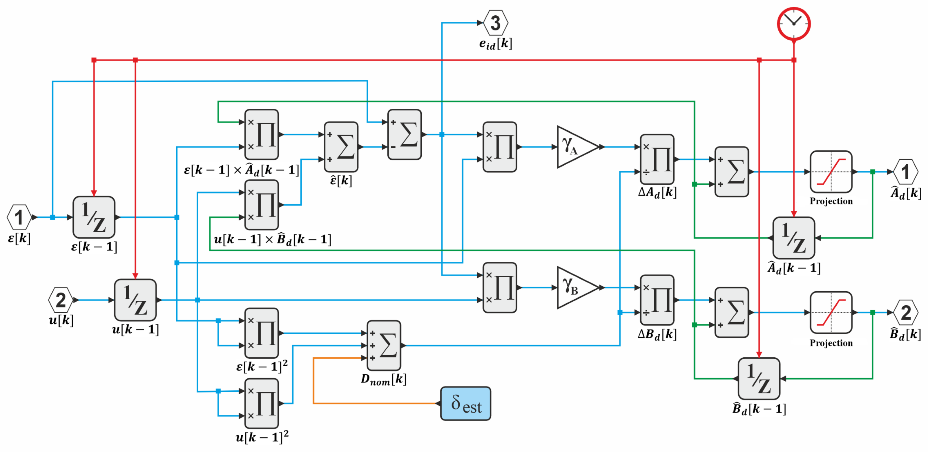
The estimator is implemented as a recursive block that uses the previous acceleration and input samples to predict the current acceleration. The prediction error adjusts the estimated coefficients, and the projection step constrains the updated values before they are used by the adaptive controllers. This implementation sequence is illustrated in Figure 6. In the Xcos implementation, the scalar projection in Equation (43) is realized using saturation blocks whose lower and upper limits are set equal to the calculated projection bounds.

3.2. Adaptive Deadbeat Acceleration Controller

Deadbeat control is a discrete time model based control method that places the assigned closed-loop roots at the origin. In a first order discrete system, this assignment gives a one sample response under the assumed plant model. The method is applied here to the inner acceleration loop using the current estimated acceleration plant coefficients [23,24,36].

The acceleration command entering the inner loop is reconstructed from the acceleration error and measured acceleration as

$${\epsilon }_c\left[k\right]=e_{\epsilon }\left[k\right]+\epsilon \left[k\right].$$

(46)

Using the estimates supplied by the online identifier, the frozen estimated first order acceleration plant at sample k is written as

$${\widehat{G}}_{\epsilon }(z,k)={\displaystyle \frac{E\left(z\right)}{U\left(z\right)}}={\displaystyle \frac{{\widehat{B}}_d\left[k\right]z^{-1}}{1-{\widehat{A}}_d\left[k\right]z^{-1}}}.$$

(47)

For deadbeat control, the desired closed-loop pulse transfer function is selected as

$$T_{db}\left(z\right)=z^{-1}.$$

(48)

For the frozen estimated model, the corresponding feedback compensator can be written in the standard form

$$C_{db}(z,k)={\displaystyle \frac{1}{{\widehat{G}}_{\epsilon }(z,k)}}{\displaystyle \frac{T_{db}\left(z\right)}{1-T_{db}\left(z\right)}}={\displaystyle \frac{1-{\widehat{A}}_d\left[k\right]z^{-1}}{{\widehat{B}}_d\left[k\right](1-z^{-1})}}.$$

(49)

The compensator form in Equation (49) gives the transfer-function representation of the controller associated with the desired deadbeat closed-loop mapping. Since $T_{db}\left(z\right)=z^{-1}$, the desired closed-loop relation is $E\left(z\right)=z^{-1}{E}_c\left(z\right)$, which is equivalent in the time domain to a one-sample acceleration response. The corresponding closed-loop characteristic root is placed at the origin,

$$z=0.$$

(50)

Therefore, the same deadbeat assignment can be implemented by enforcing

$$\epsilon [k+1]={\epsilon }_c\left[k\right].$$

(51)

The estimated acceleration model used for the implemented law is

$$\epsilon [k+1]={\widehat{A}}_d\left[k\right]\epsilon \left[k\right]+{\widehat{B}}_d\left[k\right]u_{\mathrm{req}}\left[k\right].$$

(52)

Substituting Equation (51) into Equation (52) gives

$${\widehat{A}}_d\left[k\right]\epsilon \left[k\right]+{\widehat{B}}_d\left[k\right]u_{\mathrm{req}}\left[k\right]={\epsilon }_c\left[k\right].$$

(53)

Solving Equation (53) for the required plant input gives

$$u_{\mathrm{req}}\left[k\right]={\displaystyle \frac{{\epsilon }_c\left[k\right]-{\widehat{A}}_d\left[k\right]\epsilon \left[k\right]}{{\widehat{B}}_d\left[k\right]}}.$$

(54)

The required plant input is related to the voltage command through the filtered derivative relation

$$u_{\mathrm{req}}\left[k\right]={\alpha }_{d}u[k-1]+{\beta }_d\left(V\left[k\right]-V[k-1]\right).$$

(55)

Solving Equation (55) for the voltage command gives

$$V\left[k\right]=V[k-1]+{\displaystyle \frac{1}{{\beta }_d}}\left(u_{\mathrm{req}}\left[k\right]-{\alpha }_{d}u[k-1]\right).$$

(56)

Substituting Equation (54) into Equation (56) gives the implemented adaptive deadbeat voltage law:

$$V\left[k\right]=V[k-1]+{\displaystyle \frac{1}{{\beta }_d}}\left[{\displaystyle \frac{{\epsilon }_c\left[k\right]-{\widehat{A}}_d\left[k\right]\epsilon \left[k\right]}{{\widehat{B}}_d\left[k\right]}}-{\alpha }_{d}u[k-1]\right].$$

(57)

Equation (57) computes the voltage command that imposes the deadbeat acceleration response under the current estimated plant model and the filtered derivative realization. The implemented block structure, including the previous voltage command, the filtered derivative state, and the bounded coefficient estimates, is presented in Figure 7.

3.3. Adaptive Pole Placement Acceleration Controller

Pole placement control assigns the root locations of a closed-loop characteristic equation and is a standard design approach in digital control [23,24]. Adaptive pole placement extends this idea by recalculating the controller from the current estimated plant model [29,31,37]. In this study, the method is applied to the inner acceleration loop by assigning the desired root position $p_{\epsilon }$ of the first order closed-loop acceleration characteristic equation.

Using the estimated plant in Equation (47), the desired closed-loop pulse transfer function is selected as

$$T_{pp}\left(z\right)={\displaystyle \frac{(1-p_{\epsilon })z^{-1}}{1-p_{\epsilon }{z}^{-1}}},\left|p_{\epsilon }\right|<1.$$

(58)

The denominator of Equation (58) defines the desired closed-loop characteristic equation

$$1-p_{\epsilon }{z}^{-1}=0,\mathrm{or}z-p_{\epsilon }=0.$$

(59)

Thus, $p_{\epsilon }$ denotes the assigned root position of the closed-loop acceleration characteristic equation. Stability requires this root to lie inside the unit circle.

For the frozen estimated model, the corresponding pole placement compensator can be written as

$$C_{pp}(z,k)={\displaystyle \frac{1}{{\widehat{G}}_{\epsilon }(z,k)}}{\displaystyle \frac{T_{pp}\left(z\right)}{1-T_{pp}\left(z\right)}}={\displaystyle \frac{(1-p_{\epsilon })(1-{\widehat{A}}_d\left[k\right]z^{-1})}{{\widehat{B}}_d\left[k\right](1-z^{-1})}}.$$

(60)

The compensator form in Equation (60) identifies the controller associated with the assigned characteristic root. The implemented voltage law is then obtained from the equivalent one-step model matching relation. Equation (58) gives the desired first order closed-loop acceleration response

$$\epsilon [k+1]=p_{\epsilon }\epsilon \left[k\right]+(1-p_{\epsilon }){\epsilon }_c\left[k\right].$$

(61)

The implemented pole placement law is obtained by matching the desired response in Equation (61) with the estimated plant model in Equation (52). This gives

$${\widehat{A}}_d\left[k\right]\epsilon \left[k\right]+{\widehat{B}}_d\left[k\right]u_{\mathrm{req}}\left[k\right]=p_{\epsilon }\epsilon \left[k\right]+(1-p_{\epsilon }){\epsilon }_c\left[k\right].$$

(62)

Solving Equation (62) for the required plant input gives

$$u_{\mathrm{req}}\left[k\right]={\displaystyle \frac{(p_{\epsilon }-{\widehat{A}}_d\left[k\right])\epsilon \left[k\right]+(1-p_{\epsilon }){\epsilon }_c\left[k\right]}{{\widehat{B}}_d\left[k\right]}}.$$

(63)

Using the inverse filtered derivative relation in Equation (56), the implemented voltage command becomes

$$V\left[k\right]=V[k-1]+{\displaystyle \frac{1}{{\beta }_d}}\left[{\displaystyle \frac{(p_{\epsilon }-{\widehat{A}}_d\left[k\right])\epsilon \left[k\right]+(1-p_{\epsilon }){\epsilon }_c\left[k\right]}{{\widehat{B}}_d\left[k\right]}}-{\alpha }_{d}u[k-1]\right].$$

(64)

Equation (64) defines the implemented adaptive pole placement acceleration control law. The parameter $p_{\epsilon }$ enters the voltage command as the assigned characteristic root of the inner acceleration loop. The implemented pole placement structure is shown in Figure 8.

3.4. Nominal Discrete Time Stability Interpretation of the Assigned Acceleration Dynamics

The stability interpretation in this study focuses on the nominal acceleration dynamics assigned by the adaptive deadbeat and adaptive pole placement controllers. The analysis is not intended as a complete Lyapunov proof for the full adaptive closed-loop system with projection, estimator transients, measurement noise, actuator saturation, and delay. Instead, it verifies the discrete-time stability of the acceleration dynamics imposed by the model-based inner-loop laws when the estimated model is treated as frozen at a given sample. This interpretation is consistent with the certainty-equivalence structure of the adaptive controller, in which the controller is recalculated from the currently updated parameter estimates.

For the pole placement controller, the selected value of $p_{\epsilon }$ defines the assigned root of the closed-loop acceleration characteristic equation. As shown by Equation (61), the homogeneous part of the assigned first-order acceleration response is governed by $p_{\epsilon }$. Therefore, according to the basic stability criterion for the considered discrete-time system, the pole of the assigned discrete transfer function must lie strictly inside the unit circle in the complex z-plane:

$$|p_{\epsilon }|<1.$$

(65)

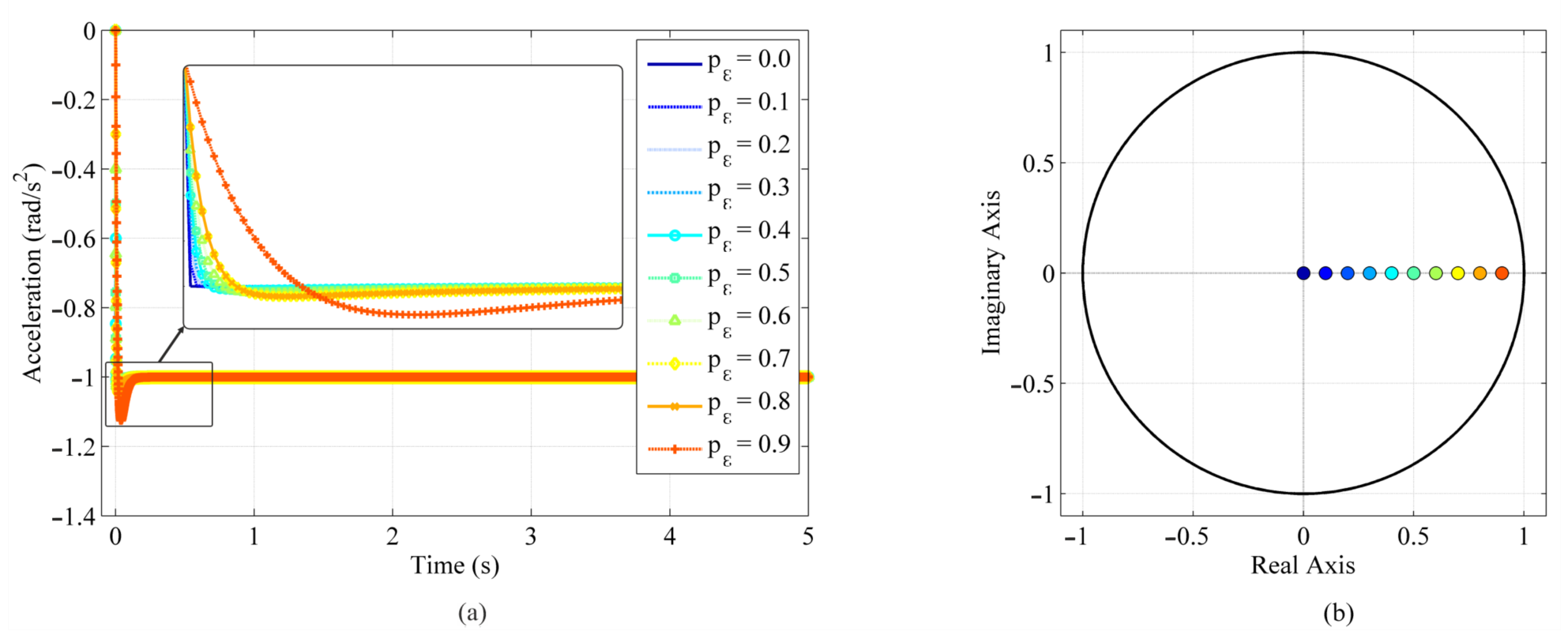
The assigned root position provides a direct interpretation of the acceleration loop dynamics. Roots closer to the origin produce faster first-order responses, while roots closer to the unit circle boundary produce slower responses with reduced aggressiveness. This relation between root position and acceleration response is summarized in Figure 9. In the numerical study, $p_{\epsilon }=0.3$ is selected to obtain a stable and moderately fast acceleration response.

The adaptive deadbeat controller corresponds to the limiting case $p_{\epsilon }=0$. Under the estimated plant model and in the absence of delay, saturation, and estimation error, this choice places the nominal assigned acceleration root at the origin. Thus, the deadbeat law gives the fastest assigned first-order acceleration response in the nominal discrete-time interpretation.

The boundedness of the adaptive parameters is supported by the projection mechanism used in the estimator. The estimates ${\widehat{A}}_d\left[k\right]$ and ${\widehat{B}}_d\left[k\right]$ are constrained to the admissible set defined in Equation (40). Therefore, the estimated parameters cannot grow without bound during the simulation. In addition, the lower bound imposed on ${\widehat{B}}_d\left[k\right]$ keeps the estimated input coefficient positive and prevents division by a very small value in the adaptive deadbeat and pole placement control laws. This keeps the implemented adaptive voltage laws well defined for all projected estimates used by the controller.

Parameter convergence should be interpreted in the usual adaptive-control sense. The normalized gradient estimator updates the model coefficients according to the prediction error, but exact convergence to the true plant parameters is not guaranteed unless the input and acceleration signals provide sufficient excitation. In the present study, exact parameter convergence is not required as the primary objective. The role of the estimator is to provide bounded online coefficients that allow the model-based inner-loop controller to maintain the assigned acceleration dynamics during the tested disturbance and tracking cases.

This stability interpretation is limited to the nominal assigned inner-loop acceleration dynamics. The complete practical response also depends on sampling time, estimator transients, numerical implementation, outer-loop interaction, disturbance level, sensor noise, voltage saturation, and computational delay. These effects are examined numerically through the disturbance and tracking tests, and they must be evaluated experimentally before applying the controller to the physical flywheel transmission test bench.

3.5. Implementation Summary

The adaptive deadbeat and adaptive pole placement controllers replace the baseline inner acceleration PI controller of the fully discrete cascaded structure. The outer velocity PI controller, the feedforward angular acceleration summation, the discrete acceleration plant, and the discrete velocity integrator remain unchanged.

The normalized gradient estimator supplies the projected online estimates ${\widehat{A}}_d\left[k\right]$ and ${\widehat{B}}_d\left[k\right]$ required by both adaptive controllers. Each adaptive controller first computes the required plant input $u_{\mathrm{req}}\left[k\right]$ from the estimated acceleration model. The voltage command $V\left[k\right]$ is then obtained by inverting the filtered derivative relation between $V\left[k\right]$ and $u\left[k\right]$. The numerical experiments in the next section compare the baseline and adaptive controllers under acceleration disturbances and segmented reference tracking conditions.

4. Numerical Experiments and Controller Comparison

Scilab/Xcos numerical experiments were used to compare the baseline digital PI controller with the adaptive deadbeat and adaptive pole-placement controllers. The simulations evaluate disturbance rejection and reference tracking while keeping the outer velocity PI controller and the feedforward angular acceleration reference unchanged. Therefore, the comparison focuses on the effect of replacing only the inner acceleration controller.

Three simulation scenarios were selected to represent operating conditions relevant to the carrier actuator. The pulse disturbance evaluates recovery after an abrupt acceleration perturbation, the sinusoidal disturbance evaluates attenuation of sustained oscillatory perturbations, and the segmented reference trajectory assesses tracking during repeated transitions between acceleration, constant-speed, deceleration, and zero-speed intervals. Although these cases do not cover all possible operating conditions of a complete flywheel energy storage system, they provide a focused comparison of disturbance rejection and reference tracking for the proposed inner-loop acceleration controllers.

The baseline digital PI controller was selected as the reference controller because it represents the fixed-gain inner-loop structure that the adaptive deadbeat and adaptive pole-placement controllers are intended to replace. The purpose is not to rank all possible advanced motor-control methods, but to evaluate whether the same cascaded acceleration–velocity architecture improves when the inner acceleration PI loop is replaced by model-based adaptive acceleration control. The comparison is supported quantitatively using acceleration and velocity RMSE and MAE indices, as reported in Section 4.3. Comparisons with additional advanced controllers, such as robust predictive control or sliding-mode-based strategies, will be considered in future experimental studies after the physical test bench and measurement chain are completed.

Table 1. Simulation parameters used in the numerical experiments.

Parameter	Symbol	Value	Unit
Motor constant	$K_m$	0.028	V s/rad
Armature resistance	$R_m$	3.3	$\mathsf{\Omega }$
Equivalent inertia	$J_{eq}$	$9.64\times {10}^{-6}$	kg m2
Sampling time	$T_s$	0.001	s
Derivative filter parameter	$T_f$	1000	s
Velocity proportional gain	$K_{p\omega }$	25	–
Velocity integral gain	$K_{i\omega }$	1	–
Acceleration proportional gain	$K_{p\epsilon }$	100	–
Acceleration integral gain	$K_{i\epsilon }$	1	–
Initial estimated coefficients	${\widehat{A}}_d\left[0\right],{\widehat{B}}_d\left[0\right]$	$A_d,B_d$	–
Adaptation gains	${\gamma }_A,{\gamma }_B$	$1\times {10}^{-5},1\times {10}^{-5}$	–
Projection bounds for ${\widehat{A}}_d$	${\widehat{A}}_{d,min},{\widehat{A}}_{d,max}$	$0.91,0.995$	–
Projection bounds for ${\widehat{B}}_d$	${\widehat{B}}_{d,min},{\widehat{B}}_{d,max}$	$0.29,2.53$	–
Assigned root of the closed-loop acceleration	$p_{\epsilon }$	0.3	–

lists the simulation parameters used in the numerical experiments. The sampling time $T_s=0.001$ s was selected as a feasible digital implementation rate for future microprocessor-based test-bench development, while the derivative filter parameter $T_f$ was used to smooth the discrete voltage derivative and reduce high-frequency amplification. The PI gains were tuned to provide a stable baseline response. For the adaptive controllers, the initial estimates were set equal to the nominal discrete plant coefficients, and the adaptation gains ${\gamma }_A$ and ${\gamma }_B$ were selected conservatively to provide gradual parameter adjustment without excessive oscillation. The projection bounds for ${\widehat{A}}_d\left[k\right]$ and ${\widehat{B}}_d\left[k\right]$ were calculated from the motor-parameter uncertainty envelope described in Section 3.1. The assigned root $p_{\epsilon }=0.3$ was selected to give a stable pole-placement response that is smoother than deadbeat control while remaining faster than a response close to the unit circle.

4.1. Acceleration Disturbance Modeling

In the initial controller development stage, the disturbance was considered as an external torque applied to the motor. However, the small equivalent inertia of the PMDC motor causes even small torque values to produce very large acceleration perturbations. For this reason, the final numerical experiments introduce the disturbance directly at the acceleration level. This disturbance acts as a bounded surrogate for equivalent acceleration effects associated with unmodeled dynamics, friction related perturbations, and carrier motion disturbances in the planetary transmission.

The acceleration disturbance is added to the output of the discrete acceleration plant before the signal is used for feedback and velocity reconstruction. Therefore, the disturbance directly affects the measured acceleration signal, while the velocity response is affected through the discrete integrator. The disturbed acceleration signal is represented as

$${\epsilon }_m\left[k\right]={\epsilon }_p\left[k\right]+{\epsilon }_d\left[k\right]$$

(66)

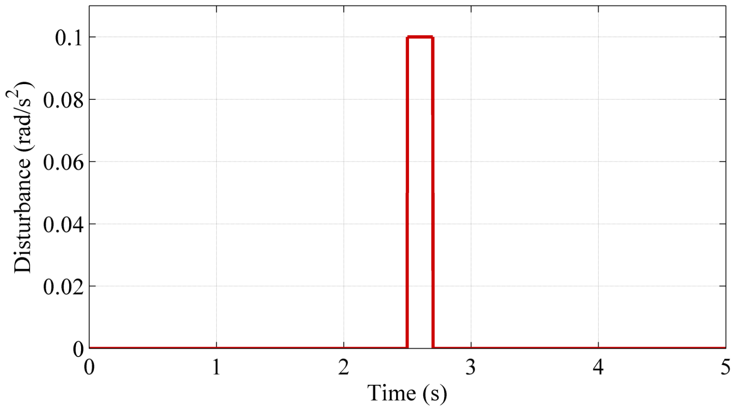
where ${\epsilon }_p\left[k\right]$ is the output of the discrete PMDC acceleration plant, ${\epsilon }_d\left[k\right]$ is the imposed acceleration disturbance, and ${\epsilon }_m\left[k\right]$ is the measured acceleration signal used by the feedback loop and velocity reconstruction. This implementation allows the disturbance response to be evaluated without introducing unrealistically large torque induced acceleration caused by the small equivalent inertia of the motor. Two disturbance types were used to evaluate disturbance rejection. The pulse disturbance represents an abrupt acceleration level perturbation, while the sinusoidal disturbance represents a continuous periodic perturbation. These two cases test different aspects of the inner acceleration loop: transient recovery after a sudden disturbance and attenuation of sustained oscillatory excitation. The pulse acceleration disturbance used in the first disturbance-rejection test is shown in Figure 10.

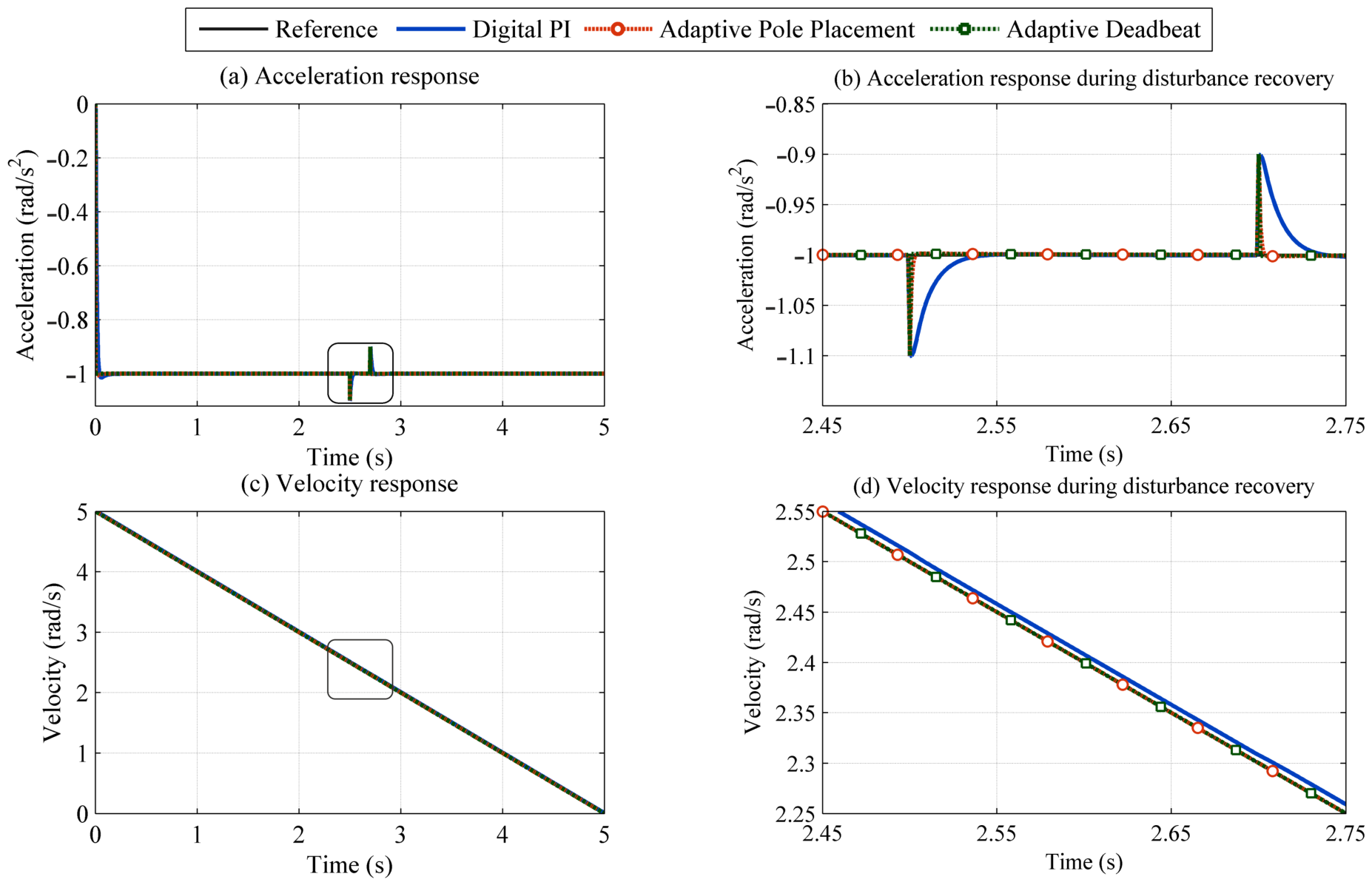
The pulse disturbance response is presented in Figure 11. This test evaluates the ability of the inner acceleration loop to recover from an abrupt perturbation. The acceleration response shows that the adaptive controllers limit the disturbance induced deviation more effectively than the baseline digital PI controller. The velocity response remains close to the reference trajectory, indicating that the disturbance effect is mainly confined to the acceleration loop and does not accumulate significantly in the reconstructed velocity.

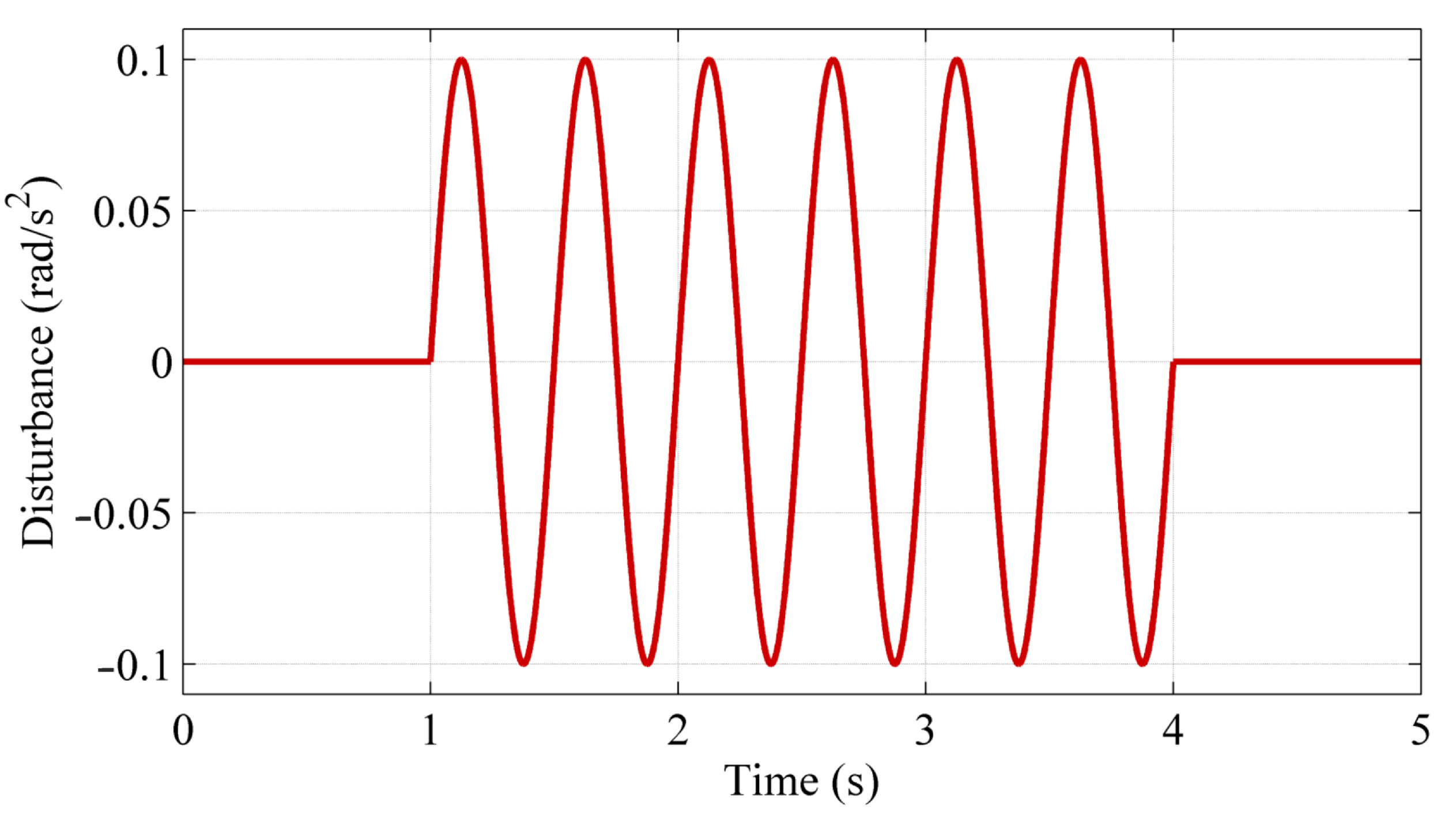
The sinusoidal disturbance depicted in Figure 12 was then applied to evaluate the controller response under sustained periodic excitation. Unlike the pulse disturbance, this case continuously perturbs the measured acceleration signal over a finite time interval and therefore tests each controller’s ability to limit oscillatory tracking error.

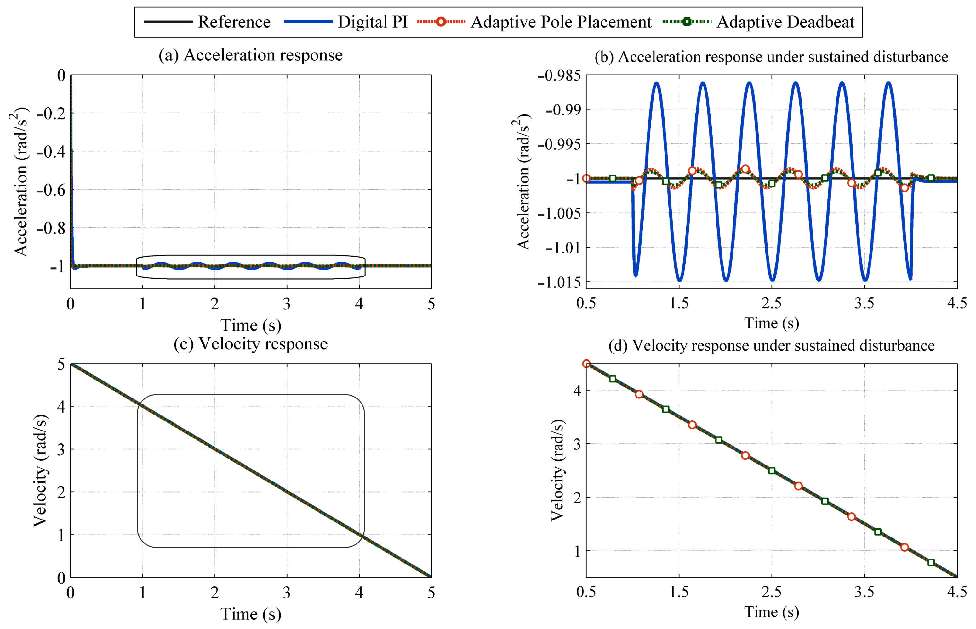
Figure 13 presents the response under sustained sinusoidal acceleration disturbance. This case is useful for evaluating whether the controller can attenuate a continuous oscillatory perturbation rather than only recover from a single transient event. The digital PI controller exhibits a more visible oscillatory component in the acceleration response, whereas the adaptive controllers reduce the disturbance induced fluctuation and preserve the velocity tracking trend.

4.2. Segmented Reference Tracking

A segmented reference trajectory was used to evaluate the controllers under a sequence of operating conditions. The reference includes constant speed operation, acceleration, deceleration, and zero speed intervals. This trajectory better represents flywheel transmission operation than a single acceleration or deceleration segment because the controller must respond to repeated changes in the commanded acceleration and velocity.

The reference trajectory is defined by the angular velocity reference ${\omega }_{ref}\left[k\right]$ and its corresponding feedforward angular acceleration reference ${\epsilon }_{ref}\left[k\right]$. During constant speed intervals, the acceleration reference is zero. During acceleration and deceleration intervals, the acceleration reference takes positive or negative constant values. The same reference trajectory was applied to the digital PI, adaptive pole placement, and adaptive deadbeat controllers.

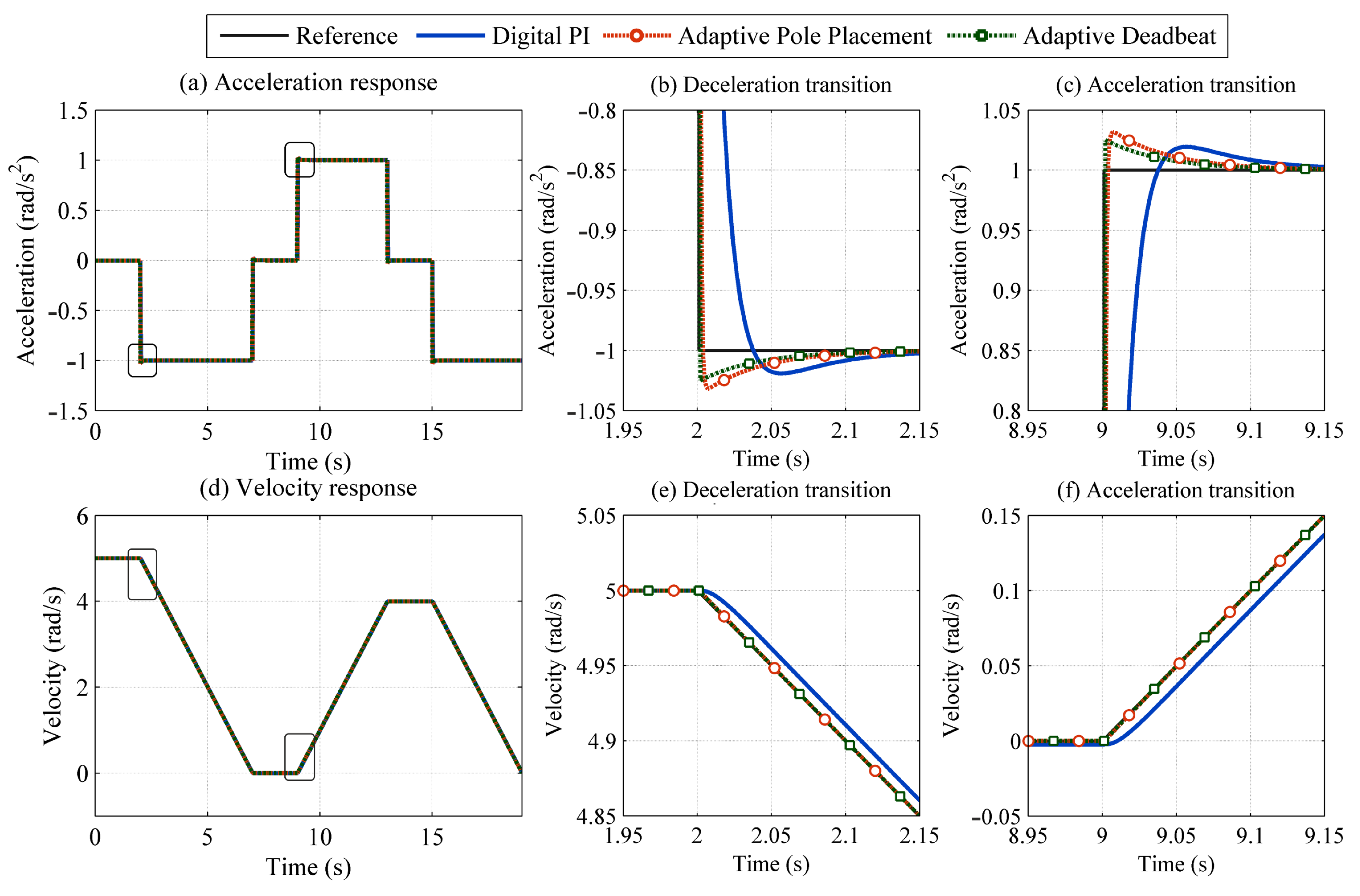
Figure 14 presents the response under the segmented reference trajectory. This test evaluates controller behavior during repeated transitions between acceleration, constant speed, deceleration, and zero speed operation. The results show that the adaptive inner loop improves the tracking of acceleration changes, which reduces the accumulated velocity error over the complete motion profile.

4.3. Quantitative Performance Indices

To provide a quantitative comparison, the root mean square error and mean absolute error were calculated for acceleration and velocity. The acceleration and velocity RMSE values are defined as

$${\mathrm{RMSE}}_{\epsilon }=\sqrt{{\displaystyle \frac{1}{N}}\sum _{k=1}^N{\left({\epsilon }_{ref}\left[k\right]-\epsilon \left[k\right]\right)}^2},{\mathrm{RMSE}}_{\omega }=\sqrt{{\displaystyle \frac{1}{N}}\sum _{k=1}^N{\left({\omega }_{ref}\left[k\right]-\omega \left[k\right]\right)}^2}.$$

(67)

The corresponding mean absolute errors are defined as

$${\mathrm{MAE}}_{\epsilon }={\displaystyle \frac{1}{N}}{\displaystyle \sum _{k=1}^N}\left|{\epsilon }_{ref}\left[k\right]-\epsilon \left[k\right]\right|,{\mathrm{MAE}}_{\omega }={\displaystyle \frac{1}{N}}{\displaystyle \sum _{k=1}^N}\left|{\omega }_{ref}\left[k\right]-\omega \left[k\right]\right|.$$

(68)

Table 2. Quantitative comparison of controller tracking performance.

Test Case	Controller	${\mathit{RMSE}}_{\mathit{\epsilon }}$ (rad/s2)	${\mathit{RMSE}}_{\mathit{\omega }}$ (rad/s)	${\mathit{MAE}}_{\mathit{\epsilon }}$ (rad/s2)	${\mathit{MAE}}_{\mathit{\omega }}$ (rad/s)
Pulse disturbance	Digital PI	$3.889\times {10}^{-2}$	$9.159\times {10}^{-3}$	$3.508\times {10}^{-3}$	$9.123\times {10}^{-3}$
Pulse disturbance	Adaptive pole placement	$1.498\times {10}^{-2}$	$3.291\times {10}^{-5}$	$4.658\times {10}^{-4}$	$8.670\times {10}^{-6}$
Pulse disturbance	Adaptive deadbeat	$1.428\times {10}^{-2}$	$1.298\times {10}^{-5}$	$2.750\times {10}^{-4}$	$3.385\times {10}^{-6}$
Sinusoidal disturbance	Digital PI	$3.929\times {10}^{-2}$	$9.216\times {10}^{-3}$	$8.197\times {10}^{-3}$	$9.165\times {10}^{-3}$
Sinusoidal disturbance	Adaptive pole placement	$1.485\times {10}^{-2}$	$6.546\times {10}^{-5}$	$9.069\times {10}^{-4}$	$4.604\times {10}^{-5}$
Sinusoidal disturbance	Adaptive deadbeat	$1.415\times {10}^{-2}$	$4.159\times {10}^{-5}$	$5.809\times {10}^{-4}$	$2.964\times {10}^{-5}$
Segmented tracking	Digital PI	$4.238\times {10}^{-2}$	$8.368\times {10}^{-3}$	$3.570\times {10}^{-3}$	$7.106\times {10}^{-3}$
Segmented tracking	Adaptive pole placement	$1.706\times {10}^{-2}$	$1.040\times {10}^{-4}$	$7.084\times {10}^{-4}$	$1.641\times {10}^{-5}$
Segmented tracking	Adaptive deadbeat	$1.632\times {10}^{-2}$	$7.304\times {10}^{-5}$	$5.268\times {10}^{-4}$	$1.149\times {10}^{-5}$

summarizes the results. The adaptive controllers reduce both acceleration and velocity tracking errors compared with the baseline digital PI controller. The improvement is especially clear in the velocity response, where the adaptive controllers reduce the tracking error by several orders of magnitude in the disturbance tests. The adaptive deadbeat controller gives the lowest error values in all test cases, while the adaptive pole placement controller also provides a substantial improvement over the digital PI controller. These results agree with the expected behavior of the two adaptive methods. Deadbeat control provides the fastest acceleration response, while pole placement provides a tunable response through the assigned characteristic root.

5. Discussion

The numerical results indicate that the inner acceleration controller strongly affects the overall cascaded response of the PMDC carrier actuator. Since the outer velocity loop and the feedforward acceleration reference remain unchanged in all tests, the observed performance differences can be attributed mainly to the inner loop control strategy. The improvement obtained with the adaptive controllers results from their direct use of the discrete acceleration plant, which allows the voltage command to be calculated from the desired acceleration dynamics rather than corrected only through fixed PI gains. This behavior is reflected in the lower acceleration and velocity error indices reported in Table 2.

The adaptive deadbeat controller gives the lowest error values because it imposes a one step acceleration response under the estimated plant model. This behavior agrees with the expected nature of deadbeat control and explains its faster recovery under the tested disturbance and tracking conditions. However, the same fast response also makes the controller more aggressive. In a physical implementation, this aggressiveness may increase sensitivity to modeling errors, sampling delay, measurement noise, and actuator constraints.

The adaptive pole placement controller provides a less aggressive alternative. By selecting the assigned characteristic root $p_{\epsilon }$, the designer can tune the compromise between response speed and smoothness. A smaller assigned root value moves the response closer to deadbeat behavior, while a larger value produces a slower but smoother acceleration response. This tunability is important for future test-bench implementation because the most accurate numerical response may not always be the most practical one when sensor noise, voltage saturation, and computational delay are present.

Improved acceleration tracking is critical at the system level, as carrier motion directly affects the torque distribution within the planetary transmission. The original flywheel-transmission concept requires the carrier torque to remain close to zero to support efficient bidirectional energy exchange between the drivetrain and the flywheel. The present study does not calculate the complete energy efficiency of the railway energy recovery system. Instead, it focuses on the actuator-level control problem that supports this mechanical operating condition. A full energy-performance assessment will require an extended electromechanical model of the transmission, flywheel, clutch, and vehicle load, together with experimental validation on the test bench.

The disturbance model used in the numerical experiments should also be interpreted carefully. In an electromechanical system, external torque is the natural physical disturbance acting on the motor shaft. However, the small equivalent inertia of the considered PMDC motor makes direct torque disturbance difficult to use in simulation, because even small torque values can produce large acceleration perturbations. For this reason, the disturbance was introduced at the acceleration level. This approach should be understood as a bounded surrogate for equivalent acceleration effects caused by unmodeled dynamics, friction-related changes, carrier-motion perturbations, and transmission irregularities. It provides a useful numerical test of disturbance rejection, but it does not replace a complete torque-based electromechanical disturbance model.

Several modeling limitations must therefore be considered before transferring the proposed controllers to the physical flywheel transmission test bench. The present numerical model does not explicitly include transmission efficiency losses, bearing friction, gear backlash, shaft compliance, clutch slip, magnetic clutch engagement dynamics, sensor noise, voltage saturation, or actuator dead zones. These effects can modify the acceleration response and may reduce the direct correspondence between the assigned discrete-time acceleration dynamics and the real system behavior. In particular, backlash and compliance can introduce hysteresis and oscillatory effects, while friction and efficiency losses can introduce load-dependent disturbances that the simplified acceleration plant model does not fully capture.

A practical limitation of the present adaptive implementation is its sensitivity to delay. Real microprocessor-based control systems introduce delay through signal acquisition, filtering, computation, communication, pulse-width modulation, and actuator response. These effects can be especially important for both adaptive deadbeat and adaptive pole-placement controllers because their control laws are based on a one-step relationship formulated for a discrete plant model. If the measured acceleration or voltage command arrives late, the controller may act on outdated information. Therefore, delay compensation and noise-aware acceleration estimation should be considered before transferring the adaptive controllers to the experimental flywheel transmission test bench.

A physical test bench for controller validation is currently under development. The planned platform is designed to reproduce friction-related disturbances acting on a rotating shaft through a disk, friction head, spring-loaded mechanism, and load-cell measurement arrangement. This setup will allow the digital PI, adaptive deadbeat, and adaptive pole-placement controllers to be compared under controlled mechanical disturbance conditions. At the present stage, the electrical and measurement subsystems are being examined, including the microprocessor-based controller, motor driver, encoder-based velocity estimation, acceleration reconstruction, sampling-time selection, and practical delay levels. Therefore, the present manuscript should be interpreted as the numerical controller-development stage preceding experimental validation. The experimental platform will be used in future work to evaluate the proposed controllers under friction, measurement noise, actuator saturation, and computational-delay conditions.

These considerations define the scope of the next experimental stage. Future implementation should quantify voltage-command limits, saturation activity, measurement-noise sensitivity, real-time computational delay, and the influence of mechanical transmission nonlinearities. These issues will determine whether the improved tracking performance observed in Scilab/Xcos can be reproduced reliably on the physical PMDC carrier actuator.

6. Conclusions

This paper developed a digital cascaded acceleration and velocity control framework for a PMDC motor used as the carrier actuator in a flywheel energy storage system with a planetary transmission. The control structure addresses the need to regulate both angular velocity and angular acceleration of the carrier, which supports operation with carrier torque close to zero in the flywheel transmission concept.

The PMDC motor was reformulated as an acceleration plant, where the input is the voltage derivative and the output is angular acceleration. This formulation allows the inner loop to control acceleration directly, while the outer loop regulates the angular velocity trajectory. Based on the fully discrete acceleration model, two adaptive inner loop controllers were developed: an adaptive deadbeat controller and an adaptive pole placement controller. Both controllers use a normalized gradient estimator with projection to update the discrete plant coefficients online and keep the estimates inside admissible bounds.

The numerical results show that both adaptive controllers reduce acceleration and velocity tracking errors compared with the baseline digital PI controller under pulse acceleration disturbance, sinusoidal acceleration disturbance, and segmented reference tracking. The adaptive deadbeat controller achieves the fastest response and the lowest error values, while the adaptive pole placement controller provides a tunable response through the assigned characteristic root.

The results indicate that adaptive inner-loop acceleration control is a promising approach for the proposed PMDC carrier actuator. However, this study remains limited to numerical simulation and should be interpreted as virtual prototyping of the control system before experimental validation. Future work will focus on implementation on the planetary-transmission flywheel test bench, with particular attention to friction-related disturbances, sensor noise, voltage saturation, actuator constraints, sampling-time selection, and computational delay.

The experimental stage will also allow the influence of the proposed carrier-motion control strategy on system-level energy exchange and transmission performance to be evaluated more directly.