A Graph Convolutional Network with Attention Mechanism for Bus Arrival Time Prediction

Abstract

Accurate prediction of bus arrival time is critical to improving transit service reliability and scheduling efficiency. The estimated time of arrival (ETA) is jointly determined by two processes, namely inter-station travel and station dwell, which are dominated by different traffic mechanisms and thus follow essentially different operating patterns. Most existing methods model the entire route in a unified way, making it difficult to account for both processes simultaneously. This paper therefore proposes a feature-separation prediction method. For inter-station travel time, which is driven by the continuous evolution of traffic flow, we design a Dual-Branch Spatio-Temporal Graph Convolutional Network (DSTGCN); its spectral graph convolution and spatial self-attention branches work together to capture road-network topology and the spatial propagation of traffic flow. For station dwell time, which follows a long-tailed distribution, we design a Spatio-Temporal Graph Convolutional Network with Transformer (STGCN-Trans) and introduce a robust loss function to suppress the effect of extreme outliers. Comparative and ablation experiments show that both models achieve the lowest RMSE, reducing it by 21.7% and 6.7% over the second-best baselines, respectively. They also remain stable under disturbances such as peak hours and extreme weather.

1. Introduction

Urban public transport is a vital means of alleviating traffic congestion and supporting green, low-carbon urban mobility, and the accurate prediction of bus arrival time is a key enabling technology for improving transit service reliability, optimizing operational scheduling, and enhancing the passenger experience [1]. The main difficulty of this task stems from the spatio-temporal heterogeneity of the bus operation process. A bus runs along a fixed route, and its overall arrival time is composed of two physical processes, namely inter-station travel and station dwell, which are governed by different factors and exhibit distinct patterns. Inter-station travel time varies relatively smoothly and is shaped mainly by traffic conditions on adjacent segments, particularly the propagation of upstream and downstream congestion. Station dwell time, by contrast, is driven by factors such as boarding and alighting demand and signal queuing; it fluctuates sharply, frequently involves sudden prolonged stops, and follows a markedly long-tailed distribution [2]. Consequently, using a single model to describe an entire route in a unified manner causes these two clearly different patterns to interfere with each other and become difficult to capture simultaneously, which limits overall prediction accuracy.

In recent years, deep learning methods represented by graph neural networks, attention mechanisms, and Transformers have advanced traffic prediction and have been introduced into bus prediction tasks [3]. For bus arrival time prediction, however, existing methods still have clear limitations. The most critical is that most of them model an entire bus route as a single sequence and rarely capture the differing spatio-temporal characteristics of inter-station travel and station dwell separately [2]. Because station dwell time is subject to the strong randomness of passenger flow and signals, exhibiting sharp fluctuations and frequent extreme values [4], such unified modeling struggles to accommodate both processes, and its prediction stability is inadequate in complex scenarios such as congested segments and sudden passenger surges. In addition, for spatial-correlation modeling, the two prevailing approaches, relying on a predefined physical graph and learning the graph structure from data, each have shortcomings, and how to combine their respective strengths remains an open question.

To address the above problems, this paper proposes a bus arrival time prediction method based on feature separation and a graph convolution-attention mechanism, using multi-source operation data from Bus Route 3 in Hohhot. Guided by the physical characteristics of bus operation, the method decouples route-level arrival time prediction into two sub-tasks, inter-station travel and station dwell, and builds a customized model for each according to its distinct spatio-temporal characteristics. For inter-station travel time, which varies smoothly and is mainly affected by spatial propagation, we construct a dual-branch spatio-temporal graph convolutional model: graph convolution captures the propagation of congestion between adjacent segments along the road network, while spatial self-attention supplements the correlation between segments that are non-adjacent yet exhibit similar operating conditions, thereby striking a balance between the predefined physical graph and the data-learned graph. For station dwell time, which fluctuates sharply and often contains extreme values, we design a spatio-temporal graph model incorporating a Transformer, combining global temporal modeling with a smoothing loss to reduce the interference of extreme stops during training. The novelty of this work lies in reformulating route-level arrival time prediction as two physically decoupled sub-tasks, inter-station travel and station dwell, and in tailoring a dedicated spatio-temporal model to the distinct dynamics of each, in place of the unified single-model formulation commonly used in prior work. The main contributions of this paper are as follows:

(1)

We propose a bus arrival time prediction framework based on the separation of inter-station travel and station dwell. Guided by the physical characteristics of bus operation, route-level prediction is decoupled into two sub-tasks, which directly address the mutual interference caused by the unified modeling adopted in existing methods.

(2)

For inter-station travel time, we construct a Dual-Branch Spatio-Temporal Graph Convolutional Network, whose two branches, graph convolution and spatial self-attention, jointly account for the physical propagation along the road network and the global implicit correlations among segments.

(3)

For station dwell time, we design a Spatio-Temporal Graph Convolutional Network with Transformer, which combines global temporal modeling with a smoothing loss to strengthen robustness against samples with sudden extreme values.

(4)

Based on a real-world bus operation dataset, we conduct multi-model comparison, spatial-heterogeneity, and ablation experiments, systematically validating the effectiveness of the proposed method and its adaptability across different scenarios.

2. Related Work

2.1. Bus Travel and Arrival Time Prediction

Research on bus travel and arrival time prediction has evolved from statistics-driven to data-driven approaches. Early methods relied largely on historical averages, statistical models, and traditional machine learning, using GPS or automatic vehicle location (AVL) data to estimate travel time through regression models such as support vector machines and neural networks. For example, Yu et al. [5] applied a support vector machine to predict bus arrival time; Gong et al. [6] built a hybrid model through the weighted fusion of historical and real-time GPS data; and other studies constructed dynamic travel time prediction models from GPS data alone [7]. Such methods are easy to implement but struggle to capture the complex nonlinear characteristics of bus operation. By contrast, deep learning has been applied to this problem: Chen et al. [8] proposed a deep belief network (DBN) for bus travel time prediction, while Hafizi et al. [9] developed a deep learning method for inter-station travel time that outperformed statistical models on real AVL data. Both achieved marked accuracy gains over traditional methods. However, these methods, which rely primarily on single time series, still cannot adequately model the spatial correlations of bus operation across the road network.

Notably, prior work has recognized that bus arrival time consists of two components, travel and dwell, which are governed by different factors. Ma et al. [2] observed that bus dwell time and travel time are driven by distinct factors and exhibit different patterns; yet few studies have modeled the two separately, and on this basis they proposed a segmented prediction method. This observation points to a long-standing gap in the field and provides the direct motivation for the feature separation framework proposed in this paper. The distinction is that our framework further tailors the modeling of each process through graph convolution and an attention mechanism, rather than relying on piecewise regression.

To explicitly model spatial dependencies, graph neural networks have recently become an important direction in bus prediction. Ma et al. [10] proposed a multi-attention graph neural network (MAGTTE) for city-wide bus travel time estimation, which incorporates a graph attention mechanism and performs well on routes with sparse data; however, it targets travel time and does not distinguish the station dwell process. Rong et al. [11] proposed an end-to-end graph attention network (GBTTE) to further characterize the spatial correlations between road segments. Qiu et al. [12] proposed a frontend-enhanced time-series prediction network (FEN-MRMGCN), which enhances front-end features through multi-relational graph convolution to predict bus arrival time and serves as an important comparison baseline in this paper. In addition, studies on bus travel time interval estimation [13] and graph-diffusion modeling of bus passenger flow [14] have extended the application of graph structures to bus-related tasks from different perspectives. Overall, these methods mostly model an entire route as a whole and still pay insufficient attention to the differentiated spatio-temporal characteristics of inter-station travel and station dwell.

2.2. Spatio-Temporal Graph Learning for Traffic Prediction

In the broader field of traffic prediction, the development of spatio-temporal graph learning provides methodological support for bus prediction. Graph convolutional networks model the road network as a graph to characterize the irregular spatial connections among network nodes [15]. Building on this, the Spatio-Temporal Graph Convolutional Network (STGCN) [16] and the Diffusion Convolutional Recurrent Neural Network (DCRNN) [17] integrate graph convolution with temporal modeling, establishing the basic paradigm of joint spatio-temporal modeling. However, such methods rely on predefined physical adjacency graphs and thus struggle to capture the implicit associations between nodes that are geographically distant yet exhibit similar operating patterns. To address this limitation, Graph WaveNet [18] introduced an adaptive adjacency matrix that learns latent spatial associations directly from data; a graph learned entirely from data, however, may weaken the physical constraints inherent in the road network. Striking a balance between the two remains a key challenge in this field, and it is precisely the problem that the dual-branch structure proposed in this paper aims to address.

To enhance the representational capacity of dependency modeling, attention mechanisms have been extensively incorporated into spatio-temporal graph networks. Graph attention networks capture spatial dependencies between nodes by assigning different weights to different neighboring nodes [19]. The Attention-Based Spatial-Temporal Graph Convolutional Network (ASTGCN) [20] and the Graph Multi-Attention Network (GMAN) [21] enhance the modeling of dynamic spatial dependencies through spatial-temporal attention and multi-attention mechanisms, respectively, while the Spatial-Temporal Self-Attention Graph Convolutional Network (STA-GCN) [22] further exploits the implicit associations between nodes. In the temporal dimension, the Transformer effectively models long-range dependencies through self-attention [23], on the basis of which decomposition-based methods for long-sequence prediction have been successively proposed [24]. More recently, models that fuse graph convolution with the Transformer have achieved strong performance in traffic flow prediction by jointly characterizing spatial topology and global temporal patterns, as exemplified by the Spatial-Temporal Gated Attention Transformer (STGAFormer) proposed by Geng et al. [25]. These advances provide a methodological foundation for modeling the complex spatio-temporal dependencies of bus operation. However, most such methods target a single traffic flow sequence and do not separately model the differentiated characteristics of the two processes, inter-station travel and station dwell.

Overall, existing research has made progress in spatio-temporal correlation modeling, yet two shortcomings remain for bus arrival prediction. First, predefined graphs and adaptive graphs each have their own limitations, and how to reconcile the two remains an open problem. Second, the differentiated spatio-temporal characteristics of inter-station travel and station dwell still lack dedicated, independent modeling. This paper addresses these two issues by handling the two processes separately through feature separation and customized dual models. In the inter-station travel model, a dual-branch structure combines the physical connectivity graph with implicit associations learned from data; in the station dwell model, the Transformer is used to capture global temporal dependencies, and a smoothing loss is introduced to accommodate the non-stationary and long-tailed characteristics of dwell time.

To summarize the reviewed literature and clarify the position of this work,

Table 1. Comparison of representative approaches for bus/traffic prediction from the perspective of route modeling and model components.

Method [Ref.]	Route Modeling	Spatial Component	Temporal Component	Separation
Traditional statistical/deep models [5,6,7,8,9]	Single route/series, non-graph	—	Regression/deep sequence	No
Ma et al. [2]	Segmented by component	—	Piecewise regression	Partial
MAGTTE [10]	Route as graph	ST graph attention	Graph attention	No
GBTTE [11]	Route as graph	ST + cross-graph attention	Attention-based	No
FEN-MRMGCN [12]	Route as graph	Multi-relational GCN	Conventional time-series	No
STGCN [16]	Predefined graph	GCN	Gated temporal conv.	No
DCRNN [17]	Predefined directed graph	Diffusion convolution	GRU encoder–decoder	No
Graph WaveNet [18]	Adaptive graph	GCN	Dilated causal conv.	No
Attention-based ST-GCNs [20,21,22]	Graph	Attention-enhanced GCN	Spatio-temporal attention	No
STGAFormer [25]	Graph	GNN	Gated temporal self-attn.	No
This work	Task-separated dual	Dual-branch: graph + attention	Attn.-temporal/Transformer	Yes

The boldfaced row indicates the method proposed in this work.

compares representative approaches from the perspectives of route modeling and the individual spatial and temporal components.

3. Materials and Methods

This paper targets the estimation of route-level bus arrival time. Based on the physical mechanisms of bus operation, the prediction task is decoupled into two processes, namely inter-station travel and station dwell, and a customized prediction model is constructed for each according to their differing spatio-temporal characteristics. This chapter presents, in turn, the problem formulation and method overview, the data and features, the model inputs, and the network architectures of the two prediction models.

3.1. Problem Formulation and Method Overview

The bus arrival time is jointly determined by the inter-station travel time and the station dwell time, whose underlying physical generation mechanisms differ fundamentally. Inter-station travel time varies relatively smoothly and exhibits strong regularity, being governed mainly by the traffic conditions of adjacent segments and, in particular, by the propagation of upstream-downstream congestion. Station dwell time, by contrast, is shaped by the combined effects of passenger-flow fluctuations, extreme weather, and concentrated transfers; it varies drastically, frequently produces sudden prolonged stops, and follows a value distribution with a pronounced long tail. To accommodate the differentiated spatio-temporal characteristics of these two processes, this paper decouples whole-route arrival time prediction into two spatio-temporal sequence prediction sub-tasks and models each separately.

The bus network is modeled as a directed graph $G=(V,E,A)$, where the node set $V=\{v_1,v_2,\dots ,v_N\}$ contains N spatial nodes, and the edge set E together with the adjacency matrix $A\in {\mathbb{R}}^{N\times N}$ characterizes the connectivity among nodes. At time step t, the feature vectors of all nodes are stacked into a graph signal matrix $X_t\in {\mathbb{R}}^{N\times F}$ at the current moment, where F is the feature dimension of a single node. Taking a historical observation window of length $T_{\mathrm{in}}$, the historical input tensor is constructed as $X=[X_{t-T_{\mathrm{in}}+1},\dots ,X_t]\in {\mathbb{R}}^{T_{\mathrm{in}}\times N\times F}$. The prediction problem is then defined as follows: given the historical tensor X and the graph structure G, a spatio-temporal mapping network $F(·)$ predicts the target state tensor $\widehat{Y}=[{\widehat{X}}_{t+1},\dots ,{\widehat{X}}_{t+T_{\mathrm{out}}}]$ over the next $T_{\mathrm{out}}$ time steps, as expressed in Equation (1).

$$\widehat{Y}=F(X,G;\Theta )$$

(1)

where $\Theta$ denotes the set of learnable parameters of the network model.

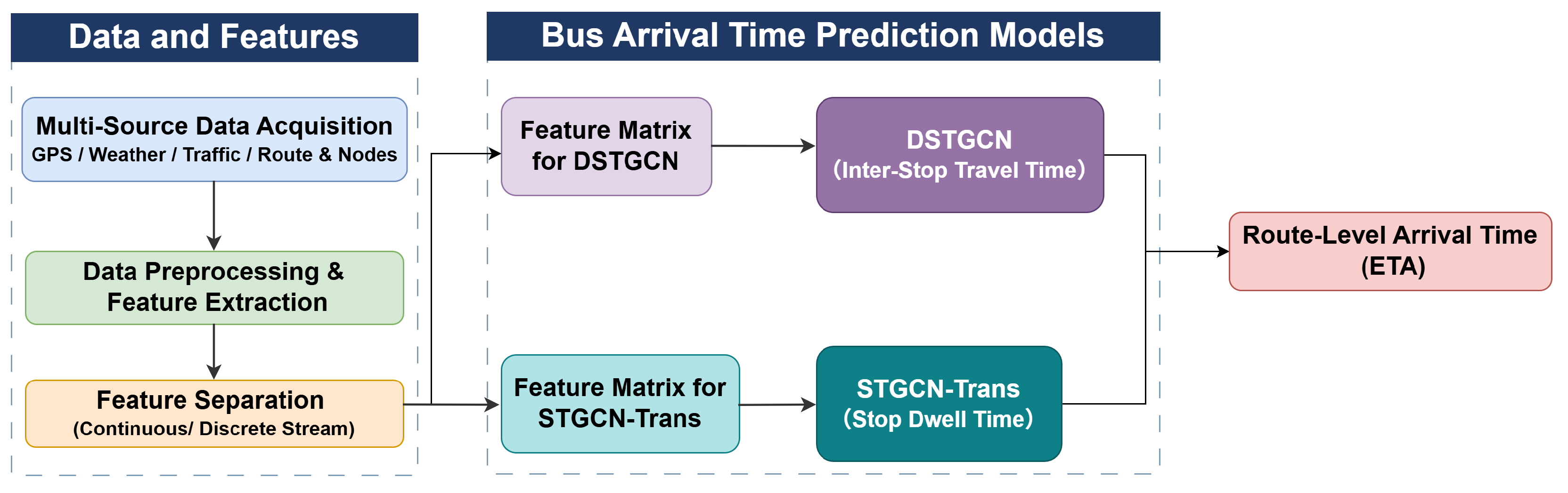
On this basis, the proposed method comprises three stages. First, the multi-source heterogeneous data are normalized and preprocessed, and a spatio-temporal feature matrix at the event granularity is extracted. Next, the input features are split by attribute into two streams: a continuous physical stream (numerical features such as historical operation time series and their periodic encodings) and a discrete semantic stream (categorical features such as weather, road conditions, and congestion level). The two streams are processed separately to prevent the discrete semantic information from being diluted by the continuous features. Finally, according to the characteristics of each task, the features are fed into two customized models: a Dual-Branch Spatio-Temporal Graph Convolutional Network for inter-station travel and a Spatio-Temporal Graph Convolutional Network with Transformer for station dwell. Both models share graph convolution, spatial self-attention, and heterogeneous feature fusion as a common modeling backbone, while adopting different structures in the temporal modeling stage tailored to the characteristics of their respective processes; each ultimately outputs its own predictions, which are combined into the whole-route arrival time. The overall framework of the method is illustrated in Figure 1.

3.2. Data and Features

This paper takes Bus Route No. 3 in Hohhot as the case study. The route comprises two independent travel directions: the inbound direction contains 36 stops and 35 segments, and the outbound direction contains 37 stops and 36 segments. The dataset comprises four types of data: vehicle-mounted GPS, route nodes, weather, and segment-level traffic conditions, obtained from the Hohhot Public Transport Corporation, the Amap (Gaode) API, and the Baidu API. Among them, the GPS data record the operating status of the vehicles themselves, while the weather and traffic data characterize the external environment affecting bus operation. The composition of each data source is summarized in

Table 2. Composition of the multi-source dataset.

Data Type	Source	Temporal Resolution	Coverage Period	Main Fields
Vehicle GPS Data	Hohhot Public Transportation Corporation	6 s	September 2024–November 2024, daily 06:00–22:00	Vehicle ID, Route ID, Longitude/Latitude, Timestamp, Direction (up/down), Next stop ID, Real-time speed, Heading angle
Route and Node Data	BusLineDesigner, Amap API	—	—	Coordinates (WGS84) of stops and intersection centers along the route (both directions), Topological sequence numbers with direction identifiers
Regional Meteorological Data	Amap Weather Service API	1 h	September 2024–November 2024, daily 06:00–22:00	Temperature, Humidity, Wind speed, Wind direction, Weather condition, Visibility
Road Traffic Condition Data	Baidu Maps Regional Traffic API	6 min	September 2024–November 2024, daily 06:00–22:00	Average traffic speed, Congestion status, Congestion index, Congestion mileage

.

The raw data were first normalized in coordinates and along the time axis, corrected through trajectory-to-road-network topology matching, and cleaned by outlier removal. Operational metrics were then extracted at the granularity of station-stop and inter-station travel events, and aggregated at 1 min and 5 min resolutions, respectively. External data, such as weather and traffic conditions, were matched strictly backward using only observations preceding the event time, so as to prevent future-information leakage. On this basis, features including temporal lags, congestion residuals, and environmental interactions were constructed, ultimately yielding a 36-dimensional spatio-temporal feature matrix. According to their physical properties, the matrix features fall into two categories (a continuous physical stream and a discrete semantic stream) whose specific composition and tensorization are detailed in Section 3.3 in conjunction with each prediction task.

3.3. Model Inputs

3.3.1. Inter-Station Travel Inputs

In terms of feature processing, the input features are split into two categories, namely a continuous physical stream and a discrete semantic stream, and differentiated processing strategies are applied according to their respective attributes to avoid the loss of semantic information.

Continuous physical stream: The extracted features include the logarithmic series of historical travel times, sine-cosine periodic encodings of the hour and the day of the week, and morning/evening peak indicators. These features are normalized to the $[0,1]$ interval via min-max scaling, providing the model with numerically stable, scale-free physical-state inputs. The min-max scaling is defined in Equation (2).

$$x_{\mathrm{norm}}={\displaystyle \frac{x-x_{min}}{x_{max}-x_{min}}}$$

(2)

where x denotes the raw value of the continuous feature to be normalized, and $x_{min}$ and $x_{max}$ are the minimum and maximum values of that feature, respectively. Through this mapping, all continuous features are projected onto the $[0,1]$ interval, eliminating the dimensional discrepancies among features and ensuring that each contributes with equal weight during model training.

Discrete semantic stream: Weather condition codes, traffic density codes, road status codes, and congestion levels are extracted and converted into discrete integers via label encoding, so as to meet the input requirements of the model’s embedding layer.

Temporal alignment and aggregation are performed at a 5 min granularity, and missing spatio-temporal entries are filled by interpolation together with forward and backward filling, so as to preserve the integrity of the temporal structure.

A sliding window of length 6 is used to construct time-series samples, where the input consists of historical multi-step features and the output is the future single-step travel time. The model finally outputs a continuous feature tensor, a discrete feature tensor, a graph-structure tensor, and a label tensor, with dimensions $B\times T\times N\times F_{\mathrm{cont}}$, $B\times T\times N\times F_{\mathrm{cat}}$, $2\times E$, $B\times N$.

For spatial graph construction, a weighted directed graph is built upon the physical topological relationships among bus segments, with nodes corresponding to travel segments. Based on the travel distance between segments, a Gaussian kernel is used to compute the edge weights, capturing the decay of spatial proximity, as defined in Equation (3).

$$W_{ij}=exp\left(-{\displaystyle \frac{\mathrm{dist}{(i,j)}^2}{2{\sigma }^2}}\right)$$

(3)

where $W_{ij}$ denotes the edge weight between segment i and segment j, $\mathrm{dist}(i,j)$ is the physical travel distance between the two segments, and $\sigma$ is the bandwidth of the Gaussian kernel, which controls the decay rate of spatial correlation. A shorter distance yields a larger edge weight, thereby reflecting spatial proximity.

In addition, a self-loop is added to each segment to preserve the propagation of its own features and to improve the stability of the graph convolution.

3.3.2. Station Dwell Inputs

In terms of feature processing, the input features are split into two categories: continuous features and discrete features. To capture the fluctuating nature of dwell time, enhanced features such as rolling statistics are extracted to characterize short-term fluctuations, while time-series data leakage is strictly avoided.

Continuous features: the logarithmic series of dwell time, periodic encodings of the hour and the day of the week, and the 3 min rolling mean, 3 min rolling standard deviation, 3 min rolling maximum, and 10 min rolling mean are extracted. All rolling statistics are computed from shifted historical data, without introducing any future information. The continuous features are then normalized to the [0, 1] interval via min-max scaling.

Discrete features: these include morning/evening peak, afternoon peak, weekend indicators, weather condition codes, traffic density codes, and road condition codes, which are converted into integer sequences through label encoding for subsequent categorical embedding learning.

Temporal alignment is performed at a 1 min granularity to construct an equally spaced spatio-temporal sequence, and missing values are handled by interpolation and filling.

A sliding window of length 6 is used to construct time-series samples, where the input consists of historical multi-step features and the output is the future single-step travel time. The model finally outputs a continuous feature tensor, a discrete feature tensor, a graph-structure tensor, and a label tensor, with dimensions $B\times T\times N\times F_{\mathrm{cont}}$, $B\times T\times N\times F_{\mathrm{cat}}$, $2\times E$, $B\times N$.

For target-distribution correction and spatial graph construction, a logarithmic transformation is applied to the target variable to address the skewness and long-tailed nature of dwell time, mapping it to an approximately normal distribution and reducing the influence of extreme values. The transformation is defined in Equation (4). After the transformation, the target is normalized so that it remains consistent with the numerical range of the inputs.

$$y_{log}=ln(1+y)$$

(4)

where y denotes the raw target value of station dwell time, and $y_{log}$ is the target value after the logarithmic transformation. The $ln(1+y)$ transformation alleviates the right-skewed distribution and long tail of dwell time, thereby mitigating the impact of extreme values on model training.

A linearly structured directed graph is constructed according to the sequential order of stops, where the nodes correspond to bus stops and adjacent stops are linked by bidirectional connections to reflect the travel association between them; a self-loop is added to each node to preserve the propagation of its own features. Considering that the travel association between adjacent stops is relatively uniform, and in order to simplify computation and improve training stability, all edge weights are set to 1. This setting meets the feature-interaction needs of the subsequent spatial modeling and is consistent with the spatial-correlation characteristics of station dwell time.

3.4. Bus Inter-Station Travel Time Prediction Model

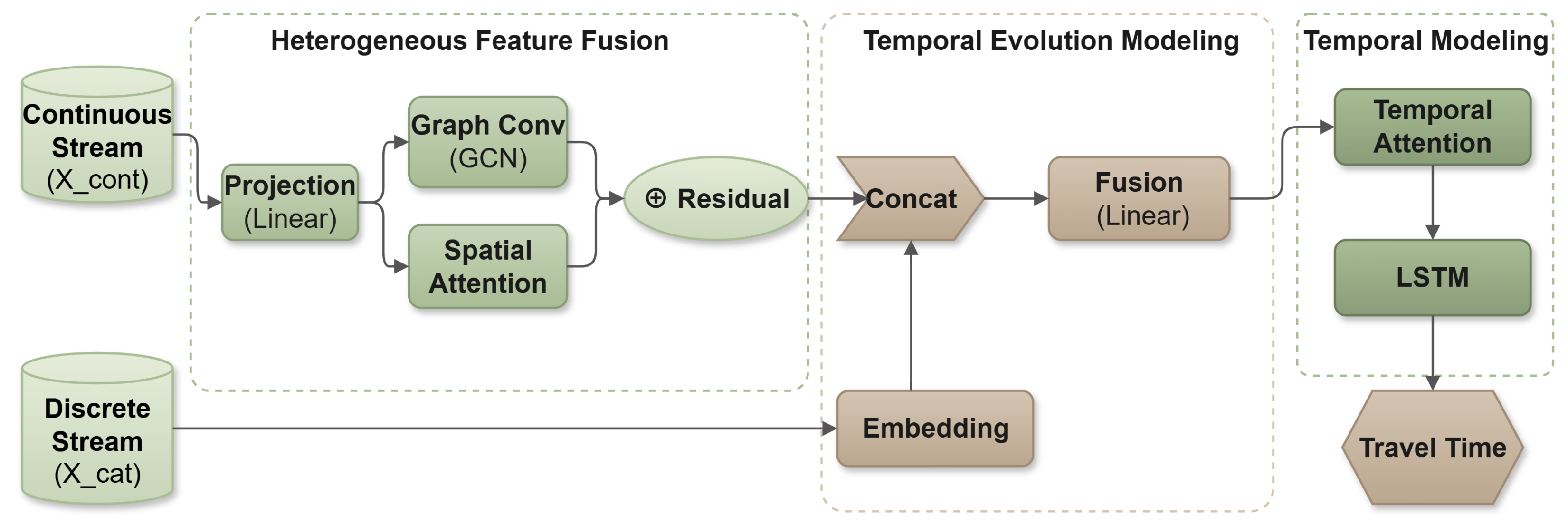
Inter-station travel time evolves smoothly and exhibits strong temporal regularity, and its spatial dependence arises both from congestion propagation between adjacent segments and from implicit associations among non-adjacent yet similar segments. To address this characteristic, and building on the separated inputs of the continuous physical stream and the discrete semantic stream, this section proposes a Dual-Branch Spatio-Temporal Graph Convolutional Network. DSTGCN is an end-to-end spatio-temporal prediction architecture comprising five modules: a multi-source input layer, a dual-branch spatial feature extraction layer, a heterogeneous feature fusion layer, a temporal evolution feature extraction layer, and a regression output layer. The overall architecture is illustrated in Figure 2.

3.4.1. Dual-Branch Spatial Feature Extraction Layer

The dual-branch spatial feature extraction layer captures the spatial dependence of the road network. It consists of three steps: feature projection, dual-branch parallel extraction, and residual fusion. Together, these steps handle the physical-connectivity constraints of the road network and the global implicit spatial associations, providing a basis for the subsequent feature fusion. Because traffic-flow diffusion in urban road networks is heterogeneous, a conventional single-graph network is prone to the limitation of a predefined local receptive field. This layer therefore adopts a dual-branch architecture that balances physical-connectivity constraints with the flexibility of global associations. A linear projection is first applied to map the input features into a high-dimensional latent space, as defined in Equation (5).

$$H^{\left(0\right)}=\mathrm{ReLU}\left(X_{\mathrm{cont}}{W}_{\mathrm{in}}+b_{\mathrm{in}}\right)$$

(5)

where $X_{\mathrm{cont}}$ is the continuous physical-stream input tensor, $W_{\mathrm{in}}$ and $b_{\mathrm{in}}$ are the weight and bias of the linear projection layer, respectively, and $H^{\left(0\right)}$ is the high-dimensional feature tensor after the initial projection.

The first branch performs local physical-dependency modeling based on spectral graph convolution. Taking the static adjacency matrix of the road network and physical-distance decay weights as priors, this branch models the linear spatial diffusion of traffic flow and the spatial coupling between adjacent segments.This computation is given in Equation (6).

$$H_{\mathrm{gcn}}=\mathrm{ReLU}\left({\tilde{D}}^{-\frac{1}{2}}\tilde{A}{\tilde{D}}^{-\frac{1}{2}}{H}^{\left(0\right)}{W}_{\mathrm{gcn}}\right)$$

(6)

where $\tilde{A}$ is the weighted adjacency matrix with self-loops added, $\tilde{D}$ is the corresponding degree matrix, and $W_{\mathrm{gcn}}$ is the weight of the graph-convolution layer.

The second branch performs global implicit-association modeling based on multi-head spatial self-attention. This branch does not rely on the physical connectivity of the road network; by computing dynamic similarities among all nodes, it identifies functional regions with similar traffic patterns (e.g., transportation hubs that are spatially distant yet share tidal morning/evening peak patterns). This computation is given in Equations (7) and (8).

$$H_{\mathrm{att}}=\mathrm{Softmax}\left({\displaystyle \frac{Q{K}^{\top }}{\sqrt{d_k}}}\right)V$$

(7)

$$H_{\mathrm{sa}}=\mathrm{LayerNorm}\left(H^{\left(0\right)}+H_{\mathrm{att}}\right)$$

(8)

where Q, K, and V are the query, key, and value matrices, respectively; $d_k$ is the feature dimension of the key matrix in the attention mechanism; $H_{\mathrm{att}}$ is the spatial-attention output feature; and $H_{\mathrm{sa}}$ is the spatial fusion feature after the residual connection and layer normalization.

Finally, the model adopts a residual aggregation strategy that adds the physical-connectivity features and the global semantic features element-wise, i.e., $H_{\mathrm{sp}}=H_{\mathrm{gcn}}+H_{\mathrm{sa}}$. This dual-branch architecture retains the constraints of the road network’s physical connectivity while providing the flexibility of global perception, thereby overcoming the limitation of a single-graph structure in capturing long-range spatial dependence.

3.4.2. Deep Heterogeneous Feature Fusion Layer

The heterogeneous feature fusion layer enables the interaction between continuous traffic-flow features and discrete environmental features, addressing the environmental-semantic dilution caused by conventional feature concatenation. Traditional spatio-temporal prediction models often concatenate high-dimensional, sparse, discrete environmental variables, such as weather and road conditions, with continuous traffic flow and normalize them jointly, which tends to dilute and even lose the environmental semantics. This layer therefore fuses the two types of heterogeneous features through discrete-feature embedding.

This architecture designs a dedicated categorical embedding space for the discrete semantic stream, mapping discrete categorical tokens into dense continuous vectors $E_{\mathrm{cat}}$ to strengthen the model’s contextual awareness. During feature interaction, a spatial-first order is followed: the spatio-temporal feature $H_{\mathrm{sp}}$ extracted by the two branches is obtained first, then concatenated with the external embedding features along the feature dimension and fed into a fully connected projection layer to complete the interaction, as defined in Equation (9).

$$H_{\mathrm{fused}}=\mathrm{ReLU}\left(\left[H_{\mathrm{sp}}\Vert E_{\mathrm{cat}}\right]W_f+b_f\right)$$

(9)

where $[H_{\mathrm{sp}}\Vert E_{\mathrm{cat}}]$ denotes the concatenation of the spatial features and the environmental embedding features along the feature dimension; $W_f$ and $b_f$ are the weight and bias of the fusion projection layer, respectively; and $H_{\mathrm{fused}}$ is the fused spatio-temporal feature tensor.

This fusion mechanism nonlinearly modulates the spatial state of traffic flow through discrete environmental factors, enabling the model to adjust the baseline for computing travel efficiency of the corresponding segment under different weather conditions.

3.4.3. Temporal Evolution Modeling Layer

The temporal evolution feature extraction layer tracks the macroscopic diffusion trend of traffic flow and addresses the local feature attenuation and response lag that traditional recurrent neural networks suffer from when handling long sequences. This layer embeds a lightweight temporal attention module in front of the LSTM to form a two-layer temporal processing structure, which reweights the features across different time frames and improves the model’s ability to capture the non-stationary evolution of traffic flow.

The temporal attention module adaptively allocates weights to the historical time steps. Let the fused spatio-temporal sequence be $H_{\mathrm{fused}}$; a feedforward neural network computes a weight score for each historical time step, which is then normalized by the Softmax function, as defined in Equations (10) and (11).

$$S=tanh\left(H_{\mathrm{fused}}{W}_{t,q}+H_{\mathrm{fused}}{W}_{t,k}\right)$$

(10)

$$\alpha =\mathrm{Softmax}\left(S{W}_{t,v}\right)$$

(11)

where $W_{t,q}$, $W_{t,k}$, and $W_{t,v}$ are learnable weight parameters; S is the intermediate weight matrix; and $\alpha$ is the normalized temporal attention weight.

This mechanism performs feature weighting through the Hadamard product, as defined in Equation (12), reweighting the feature responses at different time points. The weighted time-series features are then fed into the LSTM unit, which processes the temporal information through its internal gating mechanism and tracks the macroscopic diffusion trend of traffic flow, as defined in Equation (13). Finally, the hidden state $h_T$ at the end of the sequence is extracted, and the prediction is produced through a regression mapping, as defined in Equation (14); this alleviates the prediction lag caused by an end-to-end sequence model’s undifferentiated treatment of time steps.

$${\tilde{H}}_{\mathrm{seq}}=\alpha \odot H_{\mathrm{fused}}$$

(12)

$$h_t,c_t=\mathrm{LSTM}\left({\tilde{H}}_{\mathrm{seq}}^{\left(t\right)},h_{t-1},c_{t-1}\right)$$

(13)

$$\widehat{y}=h_T{W}_{\mathrm{out}}+b_{\mathrm{out}}$$

(14)

where ⊙ denotes the Hadamard product, i.e., element-wise matrix multiplication; $h_t$ and $c_t$ are the hidden state and cell state of the LSTM unit at time step t, respectively; $W_{\mathrm{out}}$ and $b_{\mathrm{out}}$ are the weight and bias of the output layer, respectively; and $\widehat{y}$ is the predicted inter-station travel time.

The regression output layer maps the high-dimensional features from the temporal evolution feature extraction layer to the final inter-station travel time prediction, and the model parameters are optimized via a loss function. The model adopts the MSE as the loss function, as defined in Equation (15), driving the parameters to converge by minimizing the squared error between the predicted and ground-truth values.

$$L_{\mathrm{MSE}}(y,\widehat{y})={\displaystyle \frac{1}{n}}{\displaystyle \sum _{i=1}^n}{\left(y_i-{\widehat{y}}_i\right)}^2$$

(15)

where y is the ground-truth inter-station travel time, $\widehat{y}$ is the predicted inter-station travel time, and n is the number of samples.

3.5. Bus Station Dwell Time Prediction Model

The bus arrival time is jointly determined by the inter-station travel time and the station dwell time. Compared with the smooth running state along segments, station dwell time is affected by the combined influence of passenger-flow fluctuations, extreme weather, concentrated transfers, and the use of accessibility facilities, exhibiting pronounced non-stationarity and an extreme-valued long tail. When handling such non-stationary time series, traditional recurrent neural networks suffer from long-range memory decay and gradient instability.

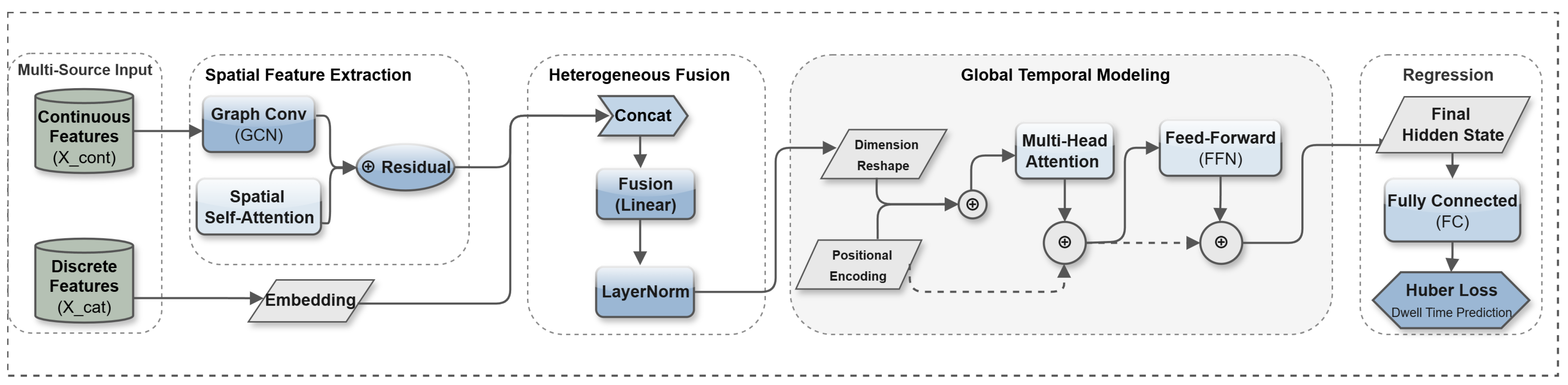
To this end, this section proposes STGCN-Trans (Spatio-Temporal Graph Convolutional Network with Transformer), an end-to-end spatio-temporal prediction architecture comprising five modules: a multi-source input layer, a spatial feature extraction layer, a heterogeneous feature fusion layer, a global temporal modeling layer, and a regression prediction layer. The framework extracts dependencies in spatio-temporal data through multi-source input fusion, feature extraction via graph convolution and spatial attention, and global temporal modeling with a Transformer, thereby completing station dwell time prediction. The overall architecture is illustrated in Figure 3.

3.5.1. Multi-Source Input Layer

The multi-source input layer is the input module of STGCN-Trans. It receives two types of feature tensors (continuous features and discrete features) and applies a differentiated processing pipeline according to the properties of each, so as to preserve complete and effective feature representations. The input features comprise continuous features $X_{\mathrm{cont}}$ and discrete features $X_{\mathrm{cat}}$, as detailed below.

Discrete features: the discrete categorical tokens are first transformed into dense continuous vectors through a categorical embedding layer, after which positional encoding (PE) is added to preserve the sequential order information, compensating for the self-attention mechanism’s limited sensitivity to absolute positions within the sequence.

Continuous features: these are fed directly into the subsequent layer, where a feedforward neural network performs the dimensional transformation and projects them into a high-dimensional latent space, meeting the input-dimension requirements of the subsequent spatial feature extraction.

Specifically, the continuous feature tensor is $X_{\mathrm{cont}}\in {\mathbb{R}}^{B\times T\times N\times F_{\mathrm{cont}}}$, where B is the batch size, T is the length of the time series, N is the number of station nodes, and $F_{\mathrm{cont}}$ is the dimension of the normalized continuous variables. After projection by the feedforward neural network, $H_{\mathrm{proj}}\in {\mathbb{R}}^{(B·T)\times N\times D}$ is obtained. The discrete feature tensor is $X_{\mathrm{cat}}\in {\mathbb{R}}^{B\times T\times N\times F_{\mathrm{cat}}}$, from which a dense continuous representation of the environmental variables, $E_{\mathrm{cat}}\in {\mathbb{R}}^{B\times T\times N\times (F_{\mathrm{cat}}·d_{\mathrm{emb}})}$, is produced after the embedding layer, where $d_{\mathrm{emb}}$ is the embedding dimension of the discrete features.

3.5.2. Spatial Feature Extraction Layer

The spatial feature extraction layer primarily extracts the complex dependencies along the spatial dimension. Through the joint processing of spectral graph convolution and spatial self-attention, it accounts for both the spatial-connectivity constraints of the road network and the global implicit associations, providing input for the subsequent feature fusion. This layer consists of three main steps: spectral graph convolution (GCN), multi-head spatial self-attention, and residual fusion, described as follows.

Spectral graph convolution (GCN): the spatial structural information of the continuous features processed by the multi-source input layer is extracted. Taking the stop adjacency graph with uniform edge weights as a prior, this branch models the spatial diffusion of dwell-related patterns between adjacent stops and captures the dependence among neighboring nodes, as defined in Equation (16).

$$H_{\mathrm{gcn}}=\mathrm{ReLU}\left({\tilde{D}}^{-\frac{1}{2}}\tilde{A}{\tilde{D}}^{-\frac{1}{2}}{H}_{\mathrm{proj}}{W}_{\mathrm{gcn}}\right)$$

(16)

where $\tilde{A}=A+I_N$ is stop adjacency matrix with self-loops added, defined on adjacent stops with uniform edge weights of 1, $\tilde{D}$ is the corresponding degree matrix, and $W_{\mathrm{gcn}}\in {\mathbb{R}}^{D\times D}$ is a learnable weight parameter.

Spatial multi-head self-attention (Spatial MSA): after the GCN layer, a multi-head spatial self-attention mechanism is introduced in parallel to overcome the feature-extraction limitation of GCN, which is constrained by physical associations in Euclidean space. By linearly mapping the query matrix Q, key matrix K, and value matrix V, it dynamically computes spatial similarities along the node dimension N, further capturing interactions along the spatial dimension and identifying implicit associations among non-adjacent stops, as defined in Equation (17).

$$H_{\mathrm{att}}=\mathrm{Softmax}\left({\displaystyle \frac{\left(H_{\mathrm{gcn}}{W}_Q\right){\left(H_{\mathrm{gcn}}{W}_K\right)}^{\top }}{\sqrt{d_k}}}\right)\left(H_{\mathrm{gcn}}{W}_V\right)$$

(17)

Residual fusion: the outputs of the GCN and the spatial attention are combined through a residual connection and layer normalization to achieve late fusion, yielding a comprehensive spatial feature representation, as defined in Equation (18). This retains the rigid constraints of physical edges while endowing the model with global perception; the feature tensor is finally reshaped to $H_{\mathrm{sa}}\in {\mathbb{R}}^{B\times T\times N\times D}$.

$$H_{\mathrm{sa}}=\mathrm{LayerNorm}\left(H_{\mathrm{gcn}}+H_{\mathrm{att}}\right)$$

(18)

3.5.3. Heterogeneous Feature Fusion Layer

The heterogeneous feature fusion layer enables the deep interaction between spatial features and discrete environmental features, avoiding the environmental-semantic dilution caused by conventional feature concatenation. External environmental factors, such as abrupt weather changes and weekends or holidays, exert a strong nonlinear modulation on bus dwell time. If high-dimensional, sparse, discrete features are forcibly concatenated with continuous traffic flow and normalized jointly, the environmental semantics are readily diluted.

To this end, this layer adopts a deep fusion strategy: the spatial state $H_{\mathrm{sa}}$ output by the spatial feature extraction layer is concatenated along the feature dimension with the environmental embedding features $E_{\mathrm{cat}}$ produced by the multi-source input layer, and fed into a fully connected projection layer to perform the cross-modal nonlinear mapping, as defined in Equation (19). The underlying rationale is to use the environmental context to modulate the base spatio-temporal features, enabling the model to adaptively account for the effects of factors such as rainfall on boarding/alighting efficiency and vehicle delays.

$$H_{\mathrm{fused}}=\mathrm{LayerNorm}\left(\mathrm{ReLU}\left(\left[H_{\mathrm{sa}}\Vert E_{\mathrm{cat}}\right]W_f+b_f\right)\right)$$

(19)

where $[H_{\mathrm{sa}}\Vert E_{\mathrm{cat}}]$ denotes the concatenation of the spatial features and the environmental embedding features along the feature dimension; $W_f$ and $b_f$ are the weight and bias of the fusion projection layer, respectively; and $H_{\mathrm{fused}}$ is the fused spatio-temporal feature tensor.

3.5.4. Global Temporal Modeling Layer

The global temporal modeling layer primarily captures the non-stationary impulse characteristics and the temporal dependencies across the input window of station dwell time, and alleviates the long-range memory decay of traditional recurrent neural networks. It mainly consists of three steps: tensor dimension reshaping, positional encoding, and temporal feature extraction by a Transformer encoder, described as follows.

First, to avoid the redundant interference of spatial-dimension computation and to focus on the temporal evolution of each individual stop, the fused tensor $H_{\mathrm{fused}}$ output by the heterogeneous feature fusion layer is permuted and reshaped: the time-step dimension T and the node dimension N are exchanged, and the batch dimension B and the node dimension N are merged, yielding a time-series-dominant independent evolution tensor $H_{\mathrm{seq}}\in {\mathbb{R}}^{T\times (B·N)\times D}$. The rationale of this permutation is to let the Transformer encoder focus on the temporal evolution within the input window of a single stop, rather than the multi-stop spatial correlation within a single time step; this matches the dominant characteristic of station dwell time, in which the temporal variation within a single stop is the primary driver of dwell-time changes, while the spatial correlation across stops is a secondary factor.

To compensate for the self-attention mechanism’s limited sensitivity to absolute positions in the sequence, an alternating sine-cosine positional encoding (PE) is introduced, as defined in Equations (20)–(22).

$$P{E}_{(pos,2i)}=sin\left({\displaystyle \frac{pos}{{10000}^{\frac{2i}{D}}}}\right)$$

(20)

$$P{E}_{(pos,2i+1)}=cos\left({\displaystyle \frac{pos}{{10000}^{\frac{2i}{D}}}}\right)$$

(21)

$$H_{\mathrm{pos}}=H_{\mathrm{seq}}+PE$$

(22)

where $pos$ is the position index within the sequence, i is the feature-dimension index, and D is the total feature dimension.

The tensor is then fed into a Transformer encoder module comprising a multi-layer perceptron and multi-head self-attention, as defined in Equation (23). Through the parallel allocation of attention weights, this module alleviates the information decay caused by the step-by-step propagation of traditional RNNs along the time axis; when an abnormally long dwell event occurs in the historical sequence, the Transformer can capture this peak feature directly across time steps, more effectively modeling transient patterns and extreme-valued outliers.

$$H_{\mathrm{trans}}=\mathrm{TransformerEncoder}\left(H_{\mathrm{pos}}\right)$$

(23)

Finally, the hidden state of the last time step of the Transformer encoder, $H_{\mathrm{trans}}^{[-1,:,:]}\in {\mathbb{R}}^{(B·N)\times D}$, is extracted as the aggregated temporal feature, providing the primary feature support for the subsequent regression prediction.

3.5.5. Regression Prediction Layer

The regression prediction layer is the output module of STGCN-Trans. Its main function is to map the temporal features from the global temporal modeling layer to the final station dwell time predictions, and to optimize the model parameters through a robust loss function. It consists of two main components: a fully connected (FC) layer and a loss function.

Fully connected (FC) layer: the last-time-step hidden state $H_{\mathrm{trans}}^{[-1,:,:]}$ extracted by the global temporal modeling layer is mapped through a linear layer and reshaped back, producing the prediction matrix $\widehat{Y}\in {\mathbb{R}}^{B\times N}$, thereby completing the conversion from features to predictions.

Loss function: given the long-tailed distribution of bus dwell time, where extreme outliers caused by factors such as equipment failures persist even after the logarithmic transformation, the smooth mean absolute error (smooth L1) is adopted as the optimization objective, so as to mitigate the gradient explosion that may arise during backpropagation.

Given the long-tailed distribution of dwell time, the smooth mean absolute error (smooth $L_1$) is adopted as the optimization objective. When the prediction residual satisfies $|y-\widehat{y}|\le \delta$, the mean squared error (MSE) is used to ensure stable convergence in the neighborhood of extreme points; when the residual exceeds $\delta$, the loss switches to the mean absolute error (MAE) branch, so that the per-sample gradient saturates at a constant magnitude instead of scaling with the error. This mitigates the gradient explosion induced by extreme samples and improves the stability of parameter updates. The threshold $\delta$ is fixed at $1.0$ as a preset hyperparameter rather than a value learned during training. This choice is consistent with the residual statistics of the training set: after the logarithmic transformation and feature scaling, the dwell-time residuals occupy a compact range, and $\delta =1.0$ lies close to their 95th percentile, which serves as the boundary between normal fluctuations and outliers.

4. Results and Discussion

Using the measured dataset from Bus Route 3 in Hohhot, this section provides a multi-dimensional quantitative evaluation of the two proposed models. The results reported here therefore establish the effectiveness of the proposed method on this route rather than universal generalizability across routes or cities, and cross-route and cross-city validation is examined as future work. We first describe the experimental setup and then, for inter-station travel prediction and station dwell prediction, respectively, verify model performance through multi-model comparison, spatial-heterogeneity analysis, and component ablation experiments.

4.1. Experimental Setup

4.1.1. Experimental Environment and Data Partitioning

The experiments were implemented with PyTorch 1.13.1 and conducted on an NVIDIA RTX 3090 GPU. Both models were trained using the Adam optimizer with an initial learning rate of 0.001 and a batch size of 64, and an early-stopping mechanism was employed to prevent overfitting. To avoid time-series data leakage, all samples were sorted in ascending order of vehicle transit time and then partitioned chronologically: the last 20% of the sequence was held out as an independent test set, and the remaining 80% was split into training and validation sets at an 8:2 ratio, resulting in a final training/validation/test partition of 64%:16%:20%. The absolute sample sizes of the training, validation, and test sets for the inbound and outbound directions of both tasks are summarized in

Table 3. Number of training, validation, and test samples for each task and direction.

Direction	Task	Total	Train (64%)	Validation (16%)	Test (20%)
Inbound	Travel (DSTGCN)	25,841	16,538	4135	5168
Outbound	Travel (DSTGCN)	25,835	16,534	4134	5167
Inbound	Dwell (STGCN-Trans)	92,649	59,295	14,824	18,530
Outbound	Dwell (STGCN-Trans)	92,640	59,290	14,822	18,528

.

4.1.2. Evaluation Metrics

Mean absolute error (MAE), root mean square error (RMSE), and mean absolute percentage error (MAPE) are adopted as the metrics for evaluating the model’s prediction performance. Each metric is computed as follows.

Mean absolute error (MAE): the average of the absolute errors between the predicted and ground-truth values, reflecting the overall bias of the predictions, as defined in Equation (24).

$$\mathrm{MAE}={\displaystyle \frac{1}{n}}{\displaystyle \sum _{i=1}^n}\left|y_i-{\widehat{y}}_i\right|$$

(24)

Root mean square error (RMSE): the square root of the mean of the squared prediction errors, which is more sensitive to large errors, as defined in Equation (25).

$$\mathrm{RMSE}=\sqrt{{\displaystyle \frac{1}{n}}{\sum }_{i=1}^n{\left(y_i-{\widehat{y}}_i\right)}^2}$$

(25)

Mean absolute percentage error (MAPE): the mean relative percentage error of the predictions, which removes the influence of differing data magnitudes across nodes, as defined in Equation (26). To avoid computational anomalies caused by a zero denominator, samples with $|y_i|<{10}^{-6}$ are excluded from the statistics.

$$\mathrm{MAPE}={\displaystyle \frac{1}{n}}{\displaystyle \sum _{i=1}^n}\left|{\displaystyle \frac{y_i-{\widehat{y}}_i}{y_i}}\right|\times 100\%$$

(26)

where n is the number of samples, $y_i$ is the ground-truth value of the i-th sample, and ${\widehat{y}}_i$ is the predicted value of the i-th sample.

4.1.3. Baseline Models for Comparison

Both prediction tasks are evaluated against a unified set of baselines. Eight representative models are selected as baselines, introduced as follows.

Historical Average (HA) [6]: based on the assumption of periodicity in time series, it produces predictions from the statistical mean of historical data over the same time period.

Support Vector Regression (SVR) [5]: it maps the input features into a high-dimensional space via a kernel function to perform nonlinear feature fitting and regression.

Bidirectional Long Short-Term Memory (Bi-LSTM) [26]: it extracts the forward and backward temporal dependencies of sequential data through a bidirectional gated recurrent structure.

LightGBM-LSTM [27]: a hybrid architecture that combines the feature-selection capability of LightGBM with the temporal feature extraction of LSTM to achieve multi-source feature fusion and time-series prediction.

BAT-Transformer [28]: built on the Transformer architecture, it captures long-range dependencies in sequential data through a temporal attention mechanism.

ISOA-DA-BiLSTM [29]: it integrates an attention mechanism with a bidirectional LSTM to achieve adaptive extraction and prediction of temporal features.

GTO-CNN-BiLSTM [30]: it combines the local feature extraction of convolutional neural networks with the temporal modeling of BiLSTM to predict spatio-temporal sequential data.

FEN-MRMGCN [12]: built on a multi-relational graph convolutional network, it captures multi-dimensional spatial correlations among road-network nodes.

All eight baselines and the two proposed models were evaluated on the same inbound and outbound bus datasets, using the same three metrics (RMSE, MAE, MAPE) and the same hardware and software environment described in Section 4.1.1. All models were optimized with the Adam optimizer under an early-stopping strategy to prevent overfitting.

4.2. Bus Arrival Travel Time Prediction Results

4.2.1. Comparison  Experiments of DSTGCN

Multi-model comparison experiments were conducted on two independent datasets for the inbound and outbound directions to verify the model’s generalization across different spatial topologies; the quantitative results are reported in

Table 4. Comparison of overall errors of multi-models for bus section travel time prediction in the inbound and outbound directions.

Model	Inbound RMSE (s)	Inbound MAE (s)	Inbound MAPE (%)	Outbound RMSE (s)	Outbound MAE (s)	Outbound MAPE (%)
HA	36.95	26.02	26.24	30.46	20.12	20.03
SVR	32.07	21.21	20.80	26.28	17.85	17.72
Bi-LSTM	27.68	17.27	20.26	22.81	13.91	14.79
LightGBM-LSTM	25.67	17.63	17.86	21.02	15.07	15.20
BAT-Transformer	22.30	14.52	14.97	18.31	11.86	13.61
GTO-CNN-BiLSTM	20.77	15.00	14.81	17.05	11.53	11.55
ISOA-DA-BiLSTM	19.58	14.30	14.12	15.84	10.42	10.31
FEN-MRMGCN	18.84	12.01	13.45	15.31	9.69	10.12
DSTGCN	14.74	10.72	12.76	12.03	8.60	9.80

Bold indicates the best performance in each column.

.

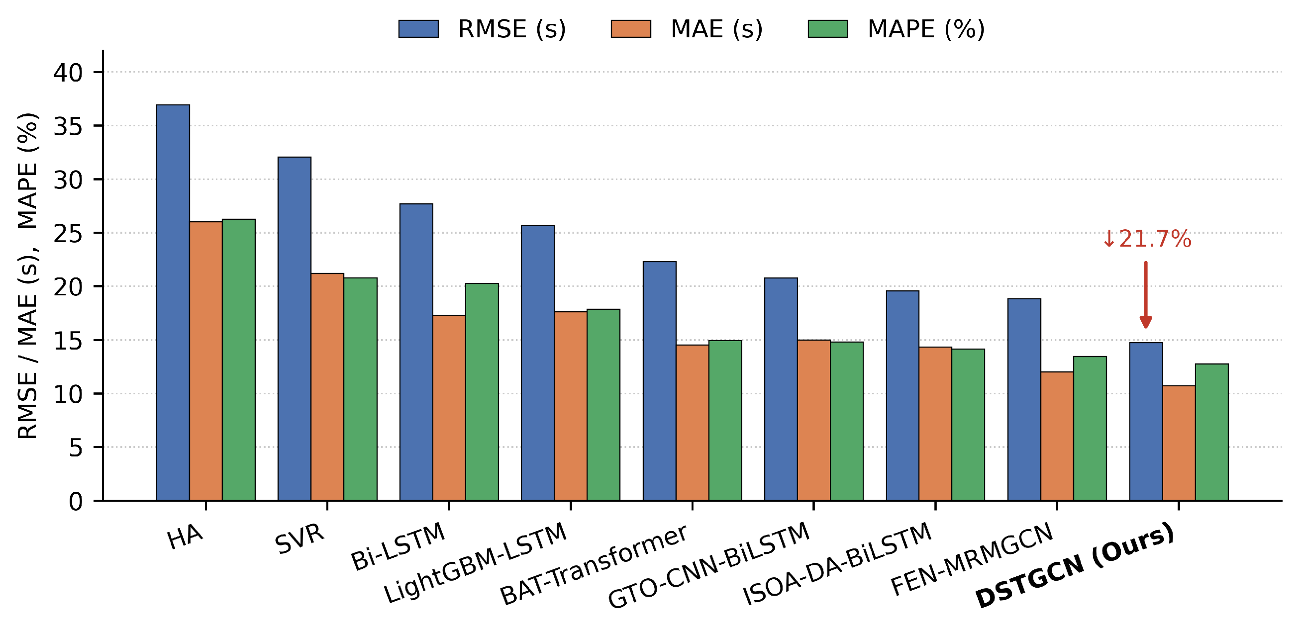
To present the performance tiers of the models and the accuracy gains of DSTGCN more intuitively, the three key metrics of all models on the inbound direction are plotted in Figure 4.

The quantitative and visual comparisons show that traditional statistical methods, constrained by their linear assumptions, struggle to fit the non-stationary fluctuations of bus travel time and thus yield relatively high errors; the inbound RMSE of the HA model reaches 36.95 s, 2.5 times that of DSTGCN. Classical deep sequence models such as Bi-LSTM can fit the nonlinear temporal trends of traffic flow, but without incorporating road-network spatial information, they cannot capture the congestion propagation between adjacent segments, and their errors remain higher than those of DSTGCN. Specifically, the inbound RMSE of Bi-LSTM is 46.7% higher than that of DSTGCN. The state-of-the-art spatio-temporal graph model FEN-MRMGCN enables spatial-correlation modeling of the road network and attains the second-best accuracy among the baselines, after DSTGCN.

DSTGCN outperforms all baselines on every metric for both directions. On the inbound dataset, it achieves an RMSE of 14.74 s, 21.7% lower than FEN-MRMGCN, with MAPE reduced by 5.1%; on the outbound dataset, it achieves an RMSE of 12.03 s and a MAPE of 9.80%, again surpassing all other baselines.

4.2.2. Spatial Heterogeneity Analysis of DSTGCN

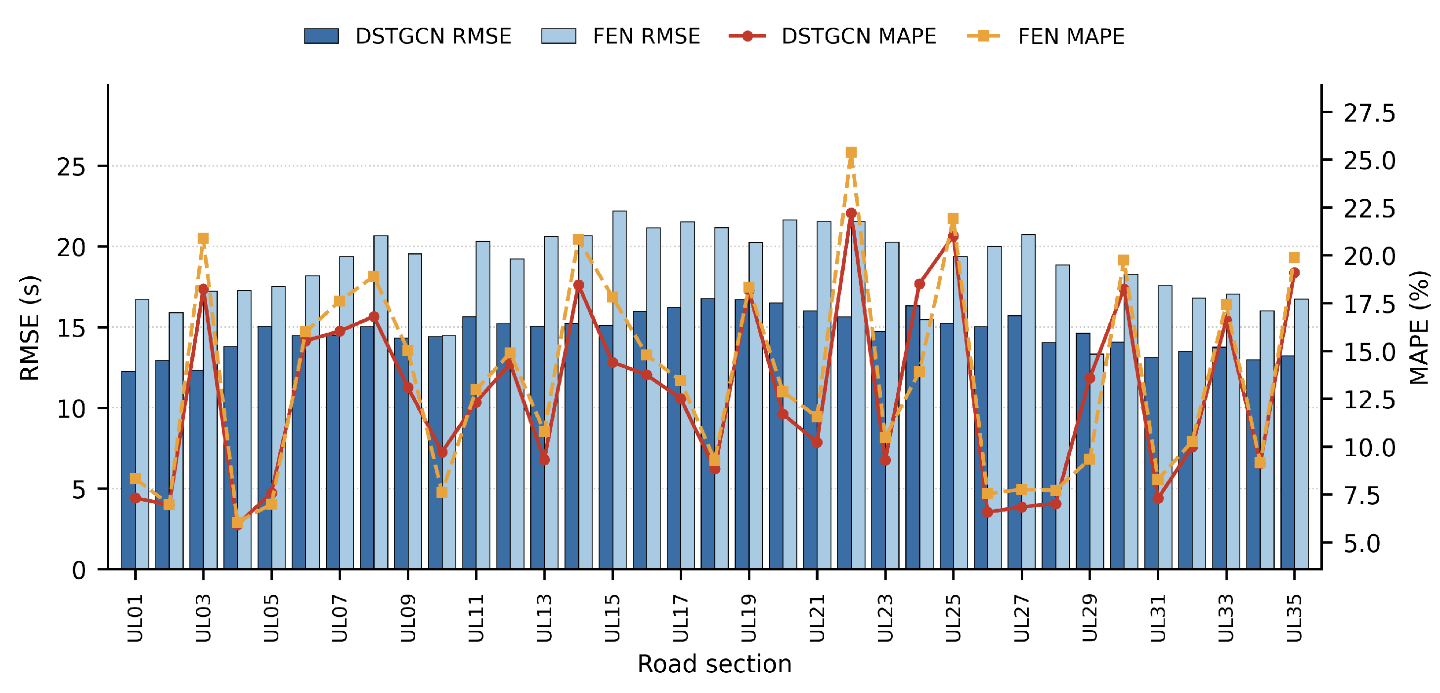
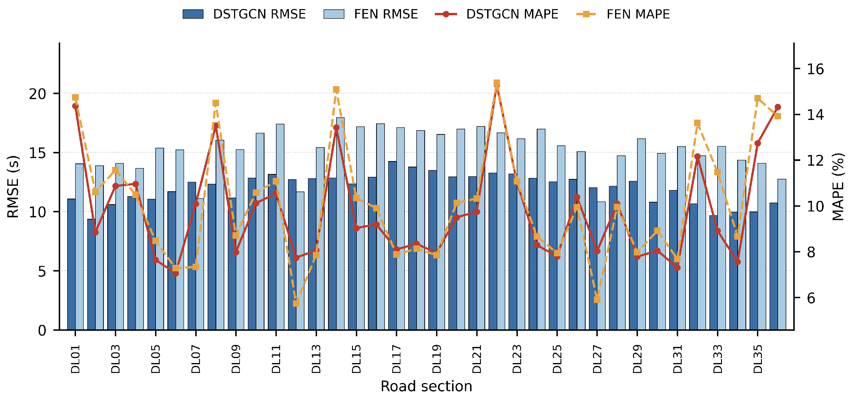
The microscopic segments of urban bus routes exhibit spatial heterogeneity, being affected by factors such as geographic location, lane configuration, surrounding commercial density, and intersection signal timing; the travel-time fluctuation characteristics differ markedly between congested and free-flowing segments. To analyze the prediction performance of DSTGCN across segments with different characteristics, the error distributions of all baseline models over the entire inbound and outbound routes were extracted and plotted as segment-wise accuracy comparisons in Figure 5 and Figure 6.

As shown in Figure 5 and Figure 6 for the inbound and outbound directions respectively, the route-wide error distributions show that DSTGCN achieves lower RMSE and MAPE than the second-best FEN-MRMGCN across all segments in both directions. On free-flowing segments with small travel-time fluctuations, DSTGCN still yields lower errors than the baselines; on segments with large fluctuations and a high probability of congestion, the error gap widens further, and this pattern holds consistently for both directions.

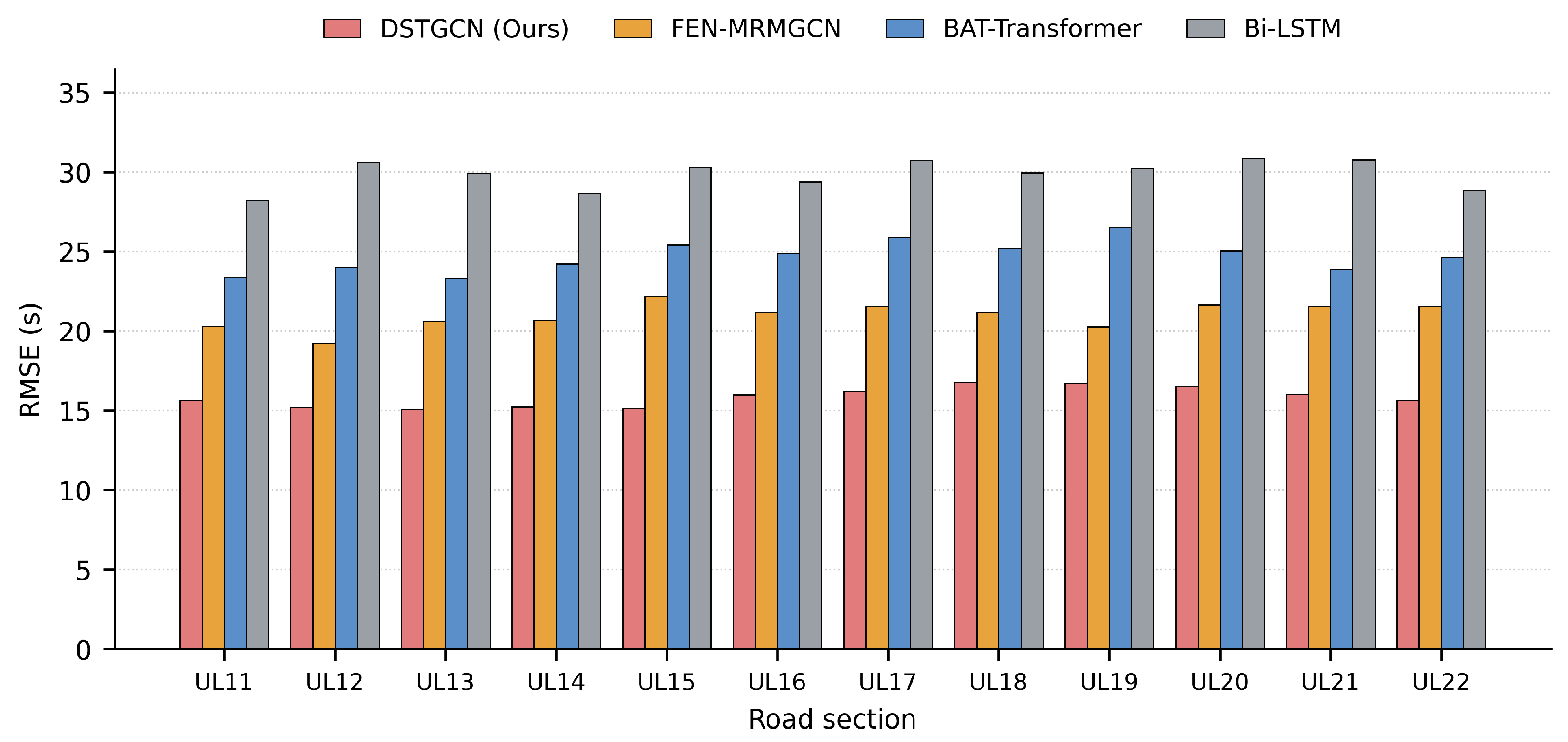
To further examine the model’s performance on congested segments, 12 representative segments that are prone to congestion in core commercial districts during morning and evening peaks were selected for a cross-model comparison; the inbound results are shown in Figure 7.

The evaluation on these representative segments shows that, on bottleneck segments in core commercial districts that are congestion-prone during peak hours (e.g., segment UL20, “Bohai Bank to No. 14 Middle School”), the purely temporal models Bi-LSTM and BAT-Transformer, which lack spatial-correlation awareness, yield RMSEs of 30.87 s and 25.05 s, respectively, and the second-best spatio-temporal model FEN-MRMGCN yields an RMSE of 21.65 s, whereas DSTGCN achieves an RMSE of 16.51 s (with a MAPE of 11.70%), 46.5% lower than Bi-LSTM and 23.7% lower than FEN-MRMGCN. These results indicate that, through the joint encoding of temporal features and spatial correlations, DSTGCN captures the congestion propagation between adjacent segments and maintains low prediction errors even on congested segments.

4.2.3. Ablation Study of DSTGCN

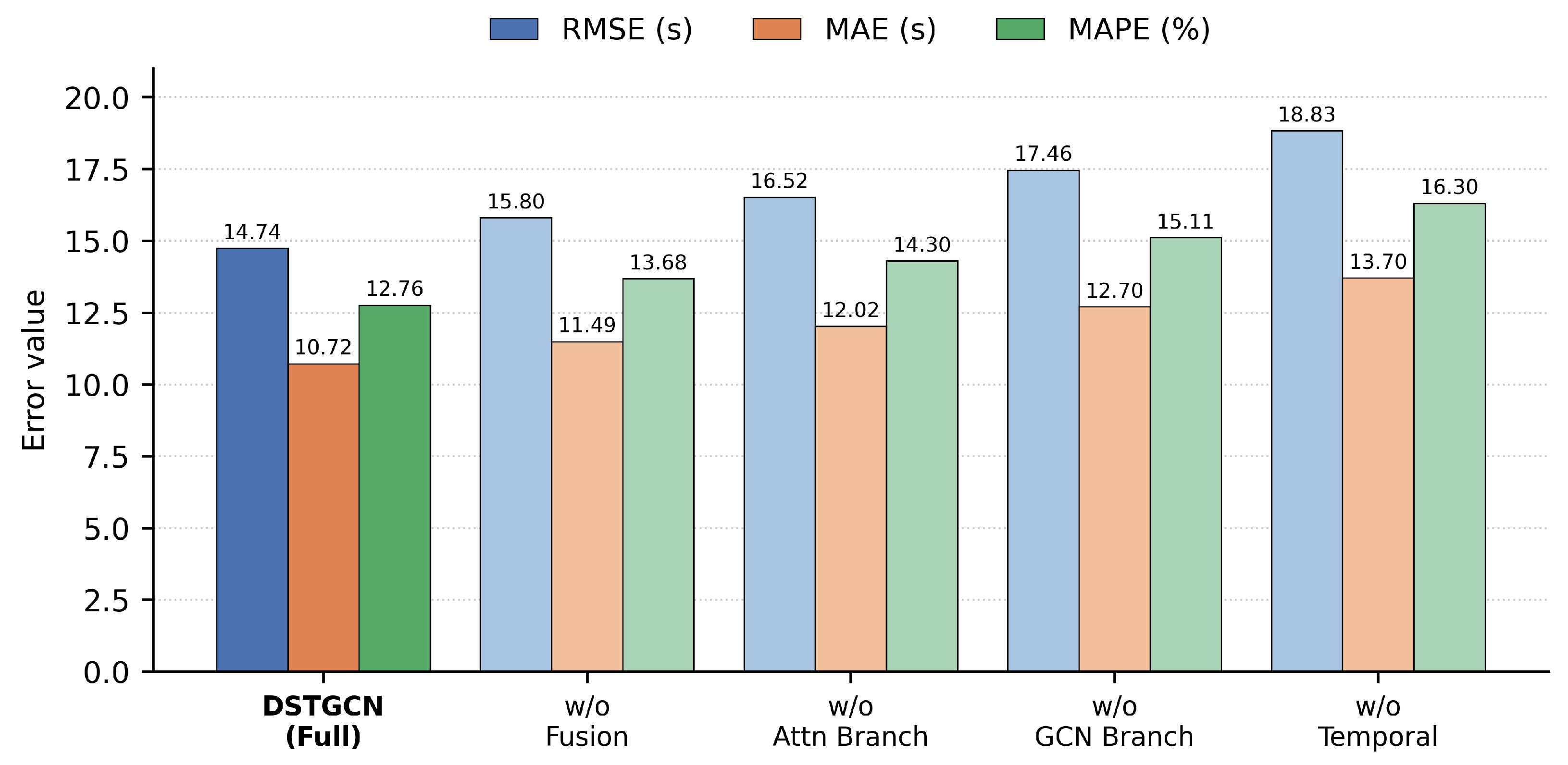
To analyze the contribution of each DSTGCN component to the prediction performance, ablation experiments were conducted following the single-variable principle. Starting from the complete DSTGCN model, four variants were constructed: w/o Temporal, which removes the temporal dependency module and retains only the spatial feature extraction; w/o GCN Branch, which removes the graph-convolution branch and thus the spatial feature extraction based on the road network’s physical connectivity; w/o Attn Branch, which removes the spatial attention branch and thus the extraction of global spatial associations; and w/o Fusion, which removes the external environmental feature fusion module and retains only the spatio-temporal trajectory features. All variants were trained and tested under identical experimental environments, datasets, and training parameters; the errors on the inbound and outbound datasets are reported in

Table 5. Error comparison of ablation experiments for the components of DSTGCN.

Model	Inbound RMSE (s)	Inbound MAE (s)	Inbound MAPE (%)	Outbound RMSE (s)	Outbound MAE (s)	Outbound MAPE (%)
w/o Temporal	18.83	13.70	16.30	15.38	10.99	12.53
w/o GCN Branch	17.46	12.70	15.11	14.27	10.20	11.62
w/o Attn Branch	16.52	12.02	14.30	13.60	9.72	11.08
w/o Fusion	15.80	11.49	13.68	12.89	9.21	10.50
DSTGCN	14.74	10.72	12.76	12.03	8.60	9.80

Bold indicates the complete model.

.

To present the performance degradation and contribution weight of each component more intuitively after its removal, the overall performance comparison for component ablation on the inbound dataset is shown in Figure 8.

The results reveal the effect of each component as follows.

(1)

Temporal dependency module. After its removal, the inbound RMSE rises from 14.74 s to 18.83 s, the inbound MAPE to 16.30%, and the outbound RMSE to 15.38 s. This is the largest error increase among all components. Inter-station travel time is affected by temporal factors such as time-of-day tidal patterns, intersection signal cycles, and station dwell durations; without this module, the model cannot extract dynamic temporal features, and the error increases accordingly.

(2)

Graph-convolution branch. After its removal, the inbound RMSE becomes 17.46 s and the outbound RMSE 14.27 s, the second-largest increase after the temporal module. This indicates that congestion states of adjacent segments in the bus network exhibit a spatial propagation effect; without this branch, the model’s ability to extract upstream-downstream congestion associations declines, and the error rises more markedly on congested segments.

(3)

Spatial attention branch. After its removal, the inbound RMSE becomes 16.52 s and the outbound RMSE 13.60 s, with a corresponding rise in error. This branch extracts global spatial associations among non-adjacent segments, complementing the coverage of the graph-convolution branch and accommodating the complex spatial dependencies of the bus network.

(4)

External environmental feature fusion module. After its removal, the inbound RMSE becomes 15.80 s and the outbound RMSE 12.89 s, both higher than those of the full model. This shows that external features such as weather, time of day, and holidays supplement environmental information not covered by the trajectory data and improve the model’s adaptability across different scenarios.

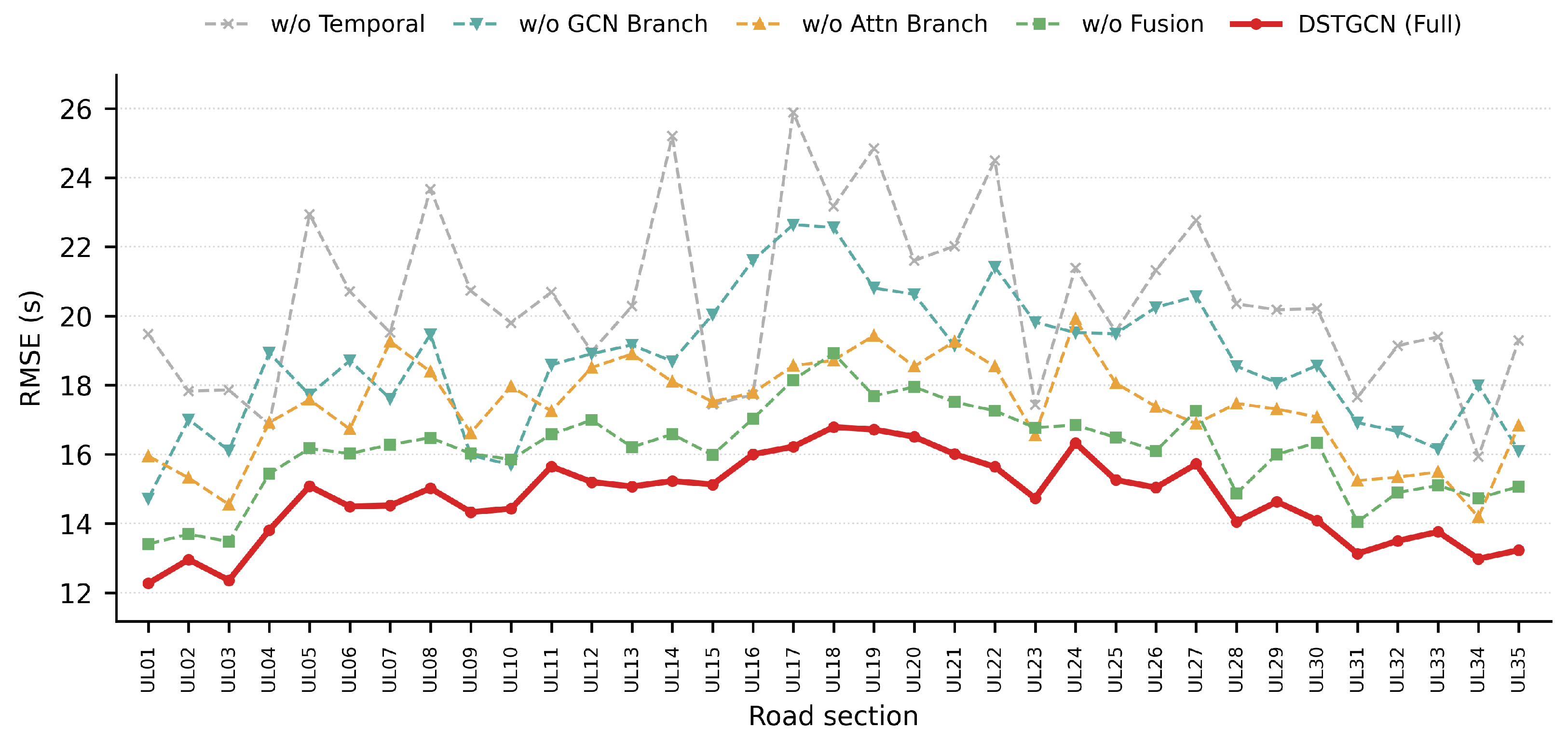
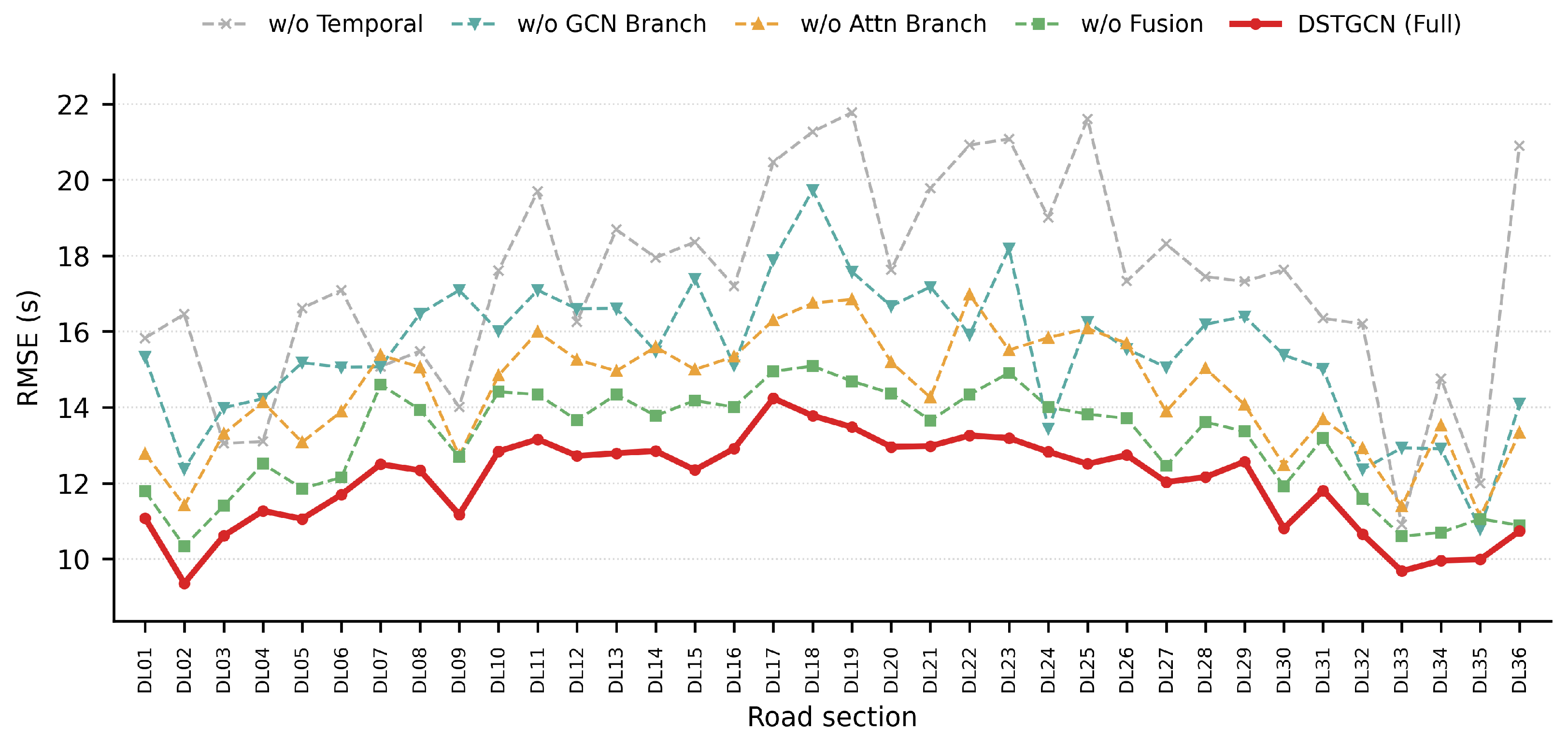
To further analyze the behavior of each component on segments with different characteristics, the RMSE distributions of the ablation variants over the entire inbound and outbound routes were extracted and plotted as segment-wise component-contribution comparisons in Figure 9 and Figure 10.

The route-wide error distributions show that the complete DSTGCN model achieves a lower RMSE than all ablation variants across the entire inbound and outbound routes. The error differences vary by scenario: on free-flowing suburban segments the gaps are small, whereas on congested segments in core commercial districts with dense intersections the gaps are larger. Among the variants, removing the temporal dependency module or the graph-convolution branch leads to a more pronounced error increase.

The analysis of typical congested segments shows that, on segments with a high frequency of peak-hour congestion such as UL14 and DL17, removing these two modules causes a larger rise in RMSE. Specifically, the variant without the temporal dependency module shows a 56.0% higher RMSE than the full model on segment UL22, and the variant without the graph-convolution branch shows a 29.6% higher RMSE on segment DL22. These results indicate that the spatio-temporal dual-branch structure of DSTGCN, through the joint encoding of temporal features and spatial associations, captures the traffic-flow variation of congested segments and maintains low prediction errors across bus segments with different characteristics.

In summary, through the coordination of its multiple components, the complete DSTGCN model maintains low prediction errors across all segments, and every component contributes positively to the prediction performance, confirming the soundness and effectiveness of the proposed architecture.

4.3. Bus Station Dwell Time Prediction Results

4.3.1. Comparison Experiments of STGCN-Trans

Multi-model comparison experiments were conducted on two independent bus-stop datasets for the inbound and outbound directions to verify the model’s generalization across different passenger-flow characteristics and spatial topologies; the overall error results of all models are reported in

Table 6. Comparison of multi-model errors for bus stop dwell time prediction in the inbound and outbound directions.

Model	Inbound RMSE (s)	Inbound MAE (s)	Inbound MAPE (%)	Outbound RMSE (s)	Outbound MAE (s)	Outbound MAPE (%)
HA	43.38	28.80	80.62	33.88	22.08	62.65
SVR	32.71	21.24	61.00	25.36	16.14	47.70
Bi-LSTM	22.05	14.30	19.40	16.85	10.84	14.88
LightGBM-LSTM	21.10	13.80	39.33	16.30	10.72	30.78
GTO-CNN-BiLSTM	19.61	12.89	35.79	15.35	9.94	28.87
ISOA-DA-BiLSTM	18.45	12.15	16.80	14.19	9.19	11.45
BAT-Transformer	15.43	9.96	13.92	11.67	7.52	9.19
FEN-MRMGCN	14.52	9.20	11.20	11.09	7.06	9.71
STGCN-Trans	13.55	9.69	12.43	10.47	7.36	10.16

Bold indicates the best performance in each column.

.

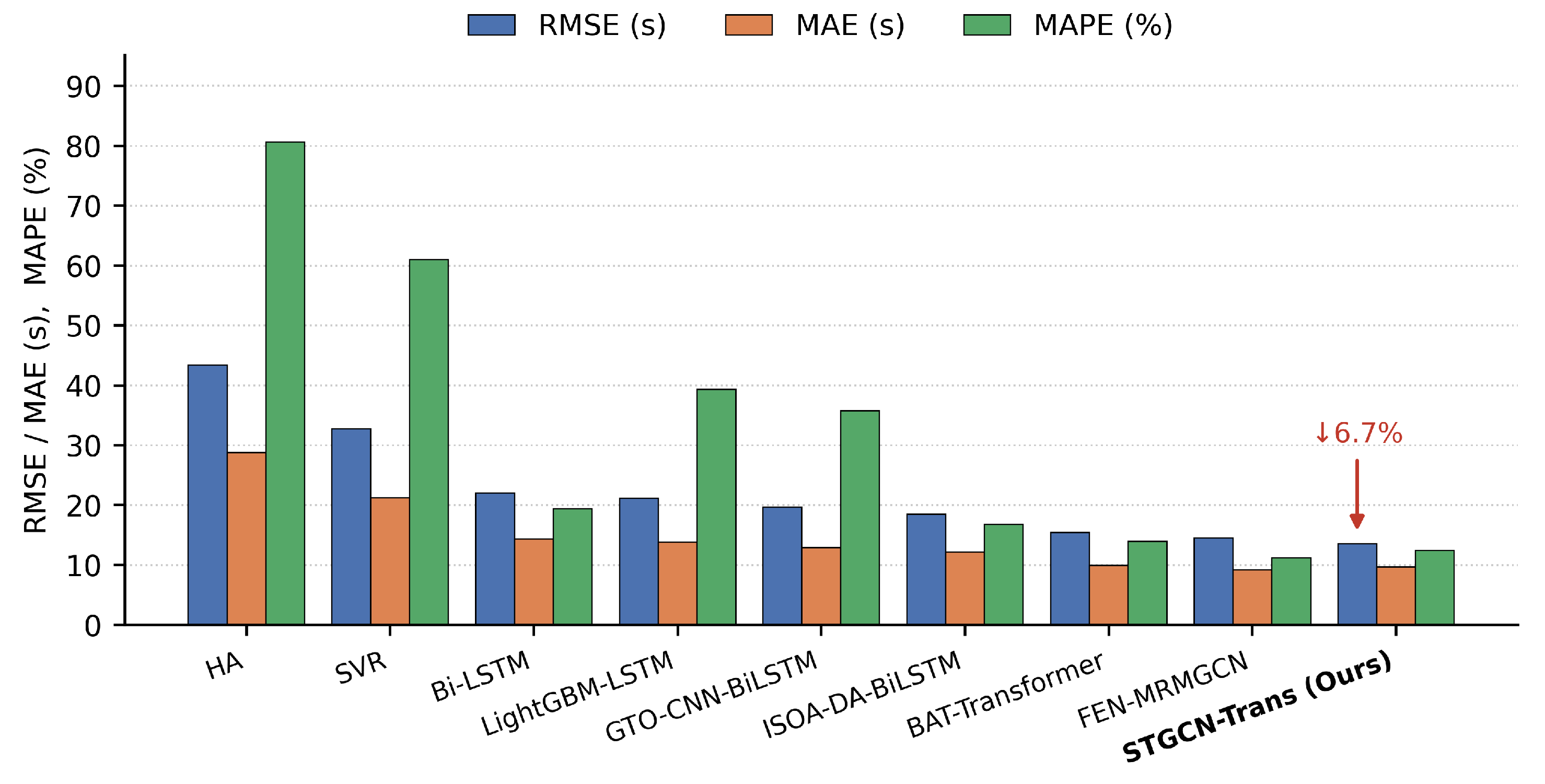
To present the performance tiers of the models and the accuracy gains of STGCN-Trans more intuitively, the three metrics of all models in the inbound direction are summarized in Figure 11.

The quantitative and visual comparisons show that traditional statistical methods, constrained by shallow linear assumptions, struggle to fit the impulsive, non-stationary fluctuations of bus dwell time and exhibit the weakest overall performance among all baselines. The inbound RMSE of the HA model reaches 43.38 s, 3.2 times that of STGCN-Trans, serving as the lower-bound benchmark for this experiment.

Classical deep sequence models such as Bi-LSTM can fit the nonlinear temporal trends of dwell time, but they lack the ability to capture spatial associations and passenger-flow coupling between stops and thus fail to account for the passenger-flow propagation between upstream and downstream stops, resulting in clear performance limitations; the inbound RMSE of Bi-LSTM is 62.7% higher than that of STGCN-Trans.

FEN-MRMGCN, the spatio-temporal graph model adopted here, possesses a certain capacity for extracting spatial-correlation features and is the second-best model in this experiment, achieving a better median fit on MAE; however, its RMSE remains relatively high, reflecting an insufficient ability to fit the extreme outliers induced by passenger-flow surges, with a pronounced accumulation of residuals.

Through spatio-temporal dual-stream joint encoding and adaptive multi-source feature fusion, STGCN-Trans attains the best performance on RMSE, which is the primary metric, for both directions: the inbound RMSE is 13.55 s, 6.7% lower than the second-best FEN-MRMGCN, and the outbound RMSE is 10.47 s, 5.6% lower than FEN-MRMGCN. These results confirm the soundness of the STGCN-Trans architecture for handling impulsive, extreme-valued data: its spatio-temporal feature extraction effectively captures the dwell-time fluctuation patterns under sudden large-passenger-flow scenarios, providing effective data support for the early intervention of bus dispatching systems against abnormal delays.

4.3.2. Spatial Heterogeneity Analysis of STGCN-Trans

Urban bus stops exhibit pronounced micro-scale spatial heterogeneity, being affected by factors such as location, surrounding land-use density, and transfer attributes. Stops in core commercial districts and at transfer hubs show marked passenger-flow surges and drastic fluctuations in vehicle operating time, constituting high-difficulty prediction scenarios; ordinary suburban stops, with stable passenger-flow supply and demand and small temporal fluctuations, are relatively easy to predict. To verify the adaptability and prediction robustness of the proposed STGCN-Trans model across heterogeneous stops, multi-model comparison experiments were conducted along three dimensions using the measured data of all inbound and outbound stops, with the results shown in Figure 12, Figure 13 and Figure 14.

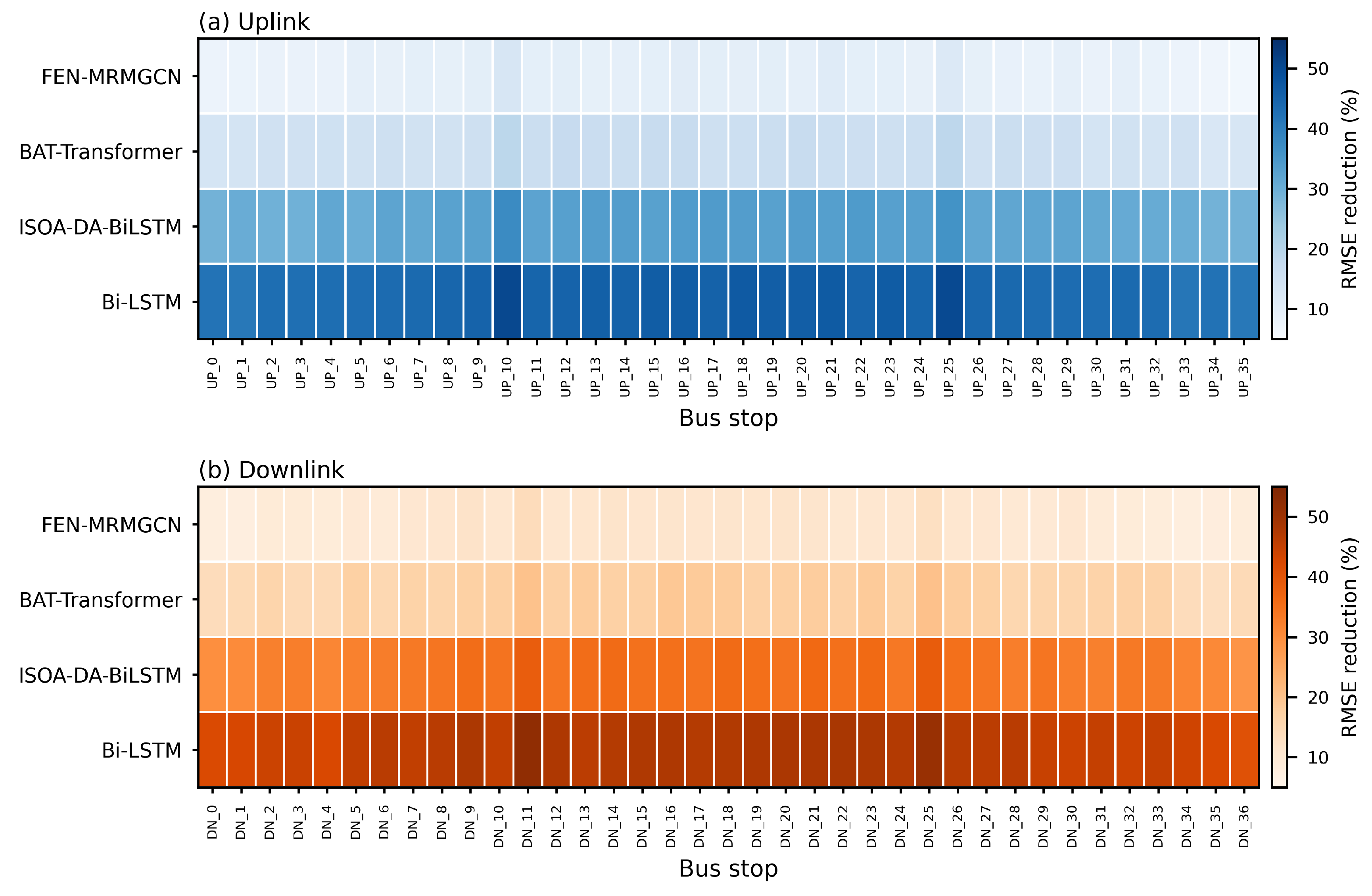
Figure 12 presents a heatmap of the RMSE improvement rate of STGCN-Trans relative to four baselines, namely FEN-MRMGCN, BAT-Transformer, ISOA-DA-BiLSTM, and Bi-LSTM.

The heat values are positive at every stop along both the inbound and outbound routes, with no case of a baseline overtaking STGCN-Trans, indicating that STGCN-Trans improves the prediction accuracy at all stops. In terms of adaptation to spatial heterogeneity, the accuracy improvement is positively correlated with the prediction difficulty of a stop: at major stops with high passenger-flow variability (e.g., outbound DN_11 Hailiang Plaza and inbound UP_16 Wanda Plaza), the RMSE reduction over Bi-LSTM reaches up to 45%, and the improvement over FEN-MRMGCN, the second-best model overall, exceeds 10%; at ordinary suburban stops with stable passenger flow, the model likewise maintains a stable positive improvement with no performance degradation, confirming its adaptability to stops of differing spatial heterogeneity.

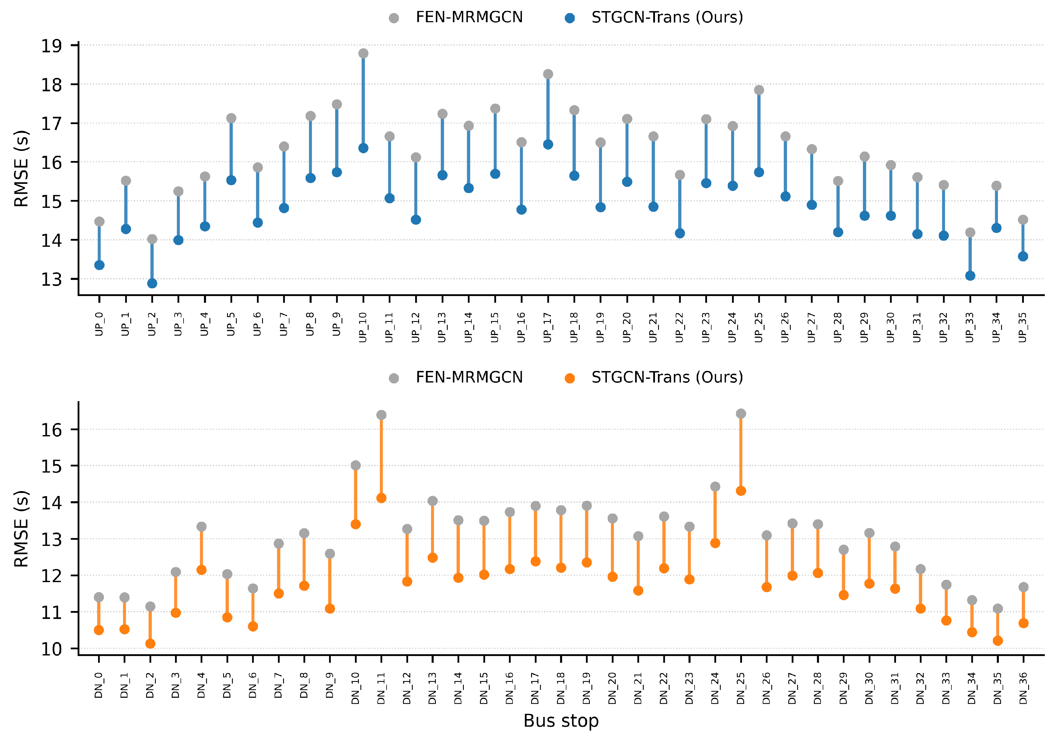
Taking FEN-MRMGCN, the best-performing baseline, as the reference, Figure 13 uses a dumbbell chart to present the absolute-error reduction achieved by the proposed model across all stops.

The results show that STGCN-Trans achieves a lower RMSE than FEN-MRMGCN at every stop along the entire route, yielding an absolute error reduction route-wide. Moreover, the magnitude of the error reduction matches the prediction difficulty of each stop: at high-variability stops with frequent passenger-flow surges (e.g., inbound UP_19 Bohai Bank and outbound DN_11 Hailiang Plaza), the absolute RMSE reduction over FEN-MRMGCN ranges from 1.66 s to 2.27 s, exceeding that at ordinary stops. This indicates that the model not only delivers stable accuracy gains route-wide but also offers stronger robustness and residual suppression in high-difficulty scenarios.

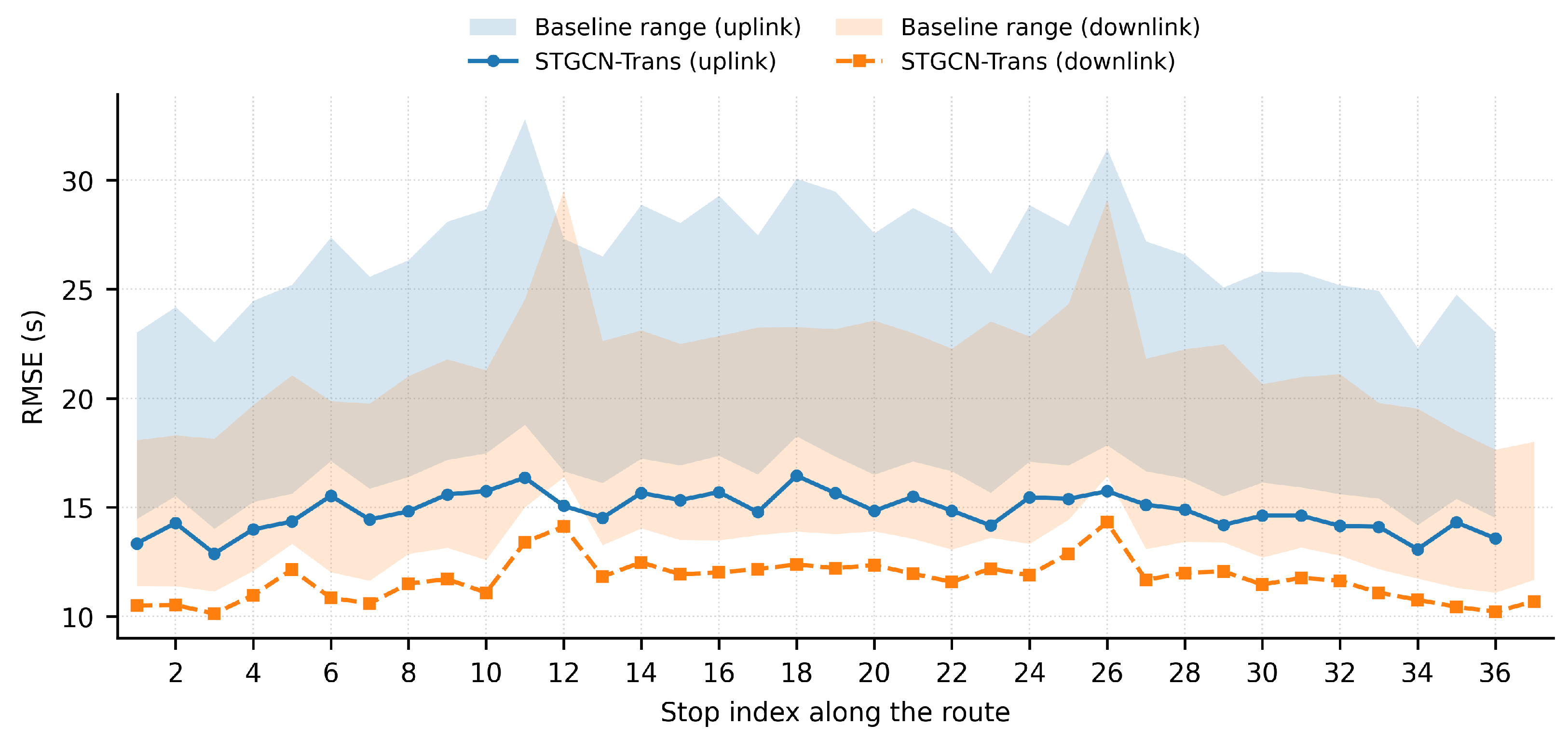
Figure 14 depicts the error evolution of STGCN-Trans along the physical spatial sequence of the bus route; the shaded band denotes the error envelope of all baseline models, reflecting the performance range of existing mainstream methods in the corresponding scenarios. The error curve of STGCN-Trans lies entirely below the lower edge of this baseline envelope, clearly separated from the baselines’ performance range: in the inbound direction, its RMSE ranges from 13.08 to 16.45 s, below the baselines’ 14.47 to 32.80 s; in the outbound direction, its RMSE ranges from 10.13 to 14.31 s, below the baselines’ 11.09 to 29.51 s. At the same time, while conforming to the spatial evolution pattern of bus operating errors, the model lowers the error peaks at major high-variability stops and reduces the fluctuation of errors route-wide, confirming its generalization and robustness in long-sequence, cross-space prediction.

In summary, through the joint deep encoding of dynamic temporal features and spatial-topological dependencies, STGCN-Trans effectively adapts to the micro-scale spatial heterogeneity of urban bus stops, achieving stable accuracy gains at both ordinary steady stops and high-variability bottleneck stops, and exhibiting robust route-wide prediction performance.

4.3.3. Ablation Study of STGCN-Trans

To examine the independent contribution, weight, and underlying mechanism of each key component of STGCN-Trans, an ablation study was conducted following the single-variable principle. Starting from the complete STGCN-Trans model, four degraded variants were constructed: w/o Temporal, which removes the temporal dependency module and retains only spatial feature extraction; w/o GCN Branch, which removes the graph-convolution branch and thus the explicit modeling of physical topology between stops; w/o Attn Branch, which removes the spatial attention branch and thus the adaptive mining of global spatial associations; and w/o Fusion, which removes the external environmental multimodal feature fusion module and retains only the spatio-temporal trajectory features. All variants were trained and tested under identical experimental environments, datasets, and training parameters; the overall errors on the inbound and outbound datasets are reported in

Table 7. Error comparison of ablation experiments for components of STGCN-Trans.

Model	Inbound RMSE (s)	Inbound MAE (s)	Inbound MAPE (%)	Outbound RMSE (s)	Outbound MAE (s)	Outbound MAPE (%)
w/o Temporal	17.30	12.37	15.87	13.41	9.43	13.01
w/o GCN Branch	16.00	11.44	14.67	12.45	8.75	12.08
w/o Attn Branch	15.19	10.86	13.93	11.80	8.30	11.45
w/o Fusion	14.52	10.39	13.32	11.22	7.88	10.88
STGCN-Trans	13.55	9.69	12.43	10.47	7.36	10.16

Bold indicates the complete model.

.

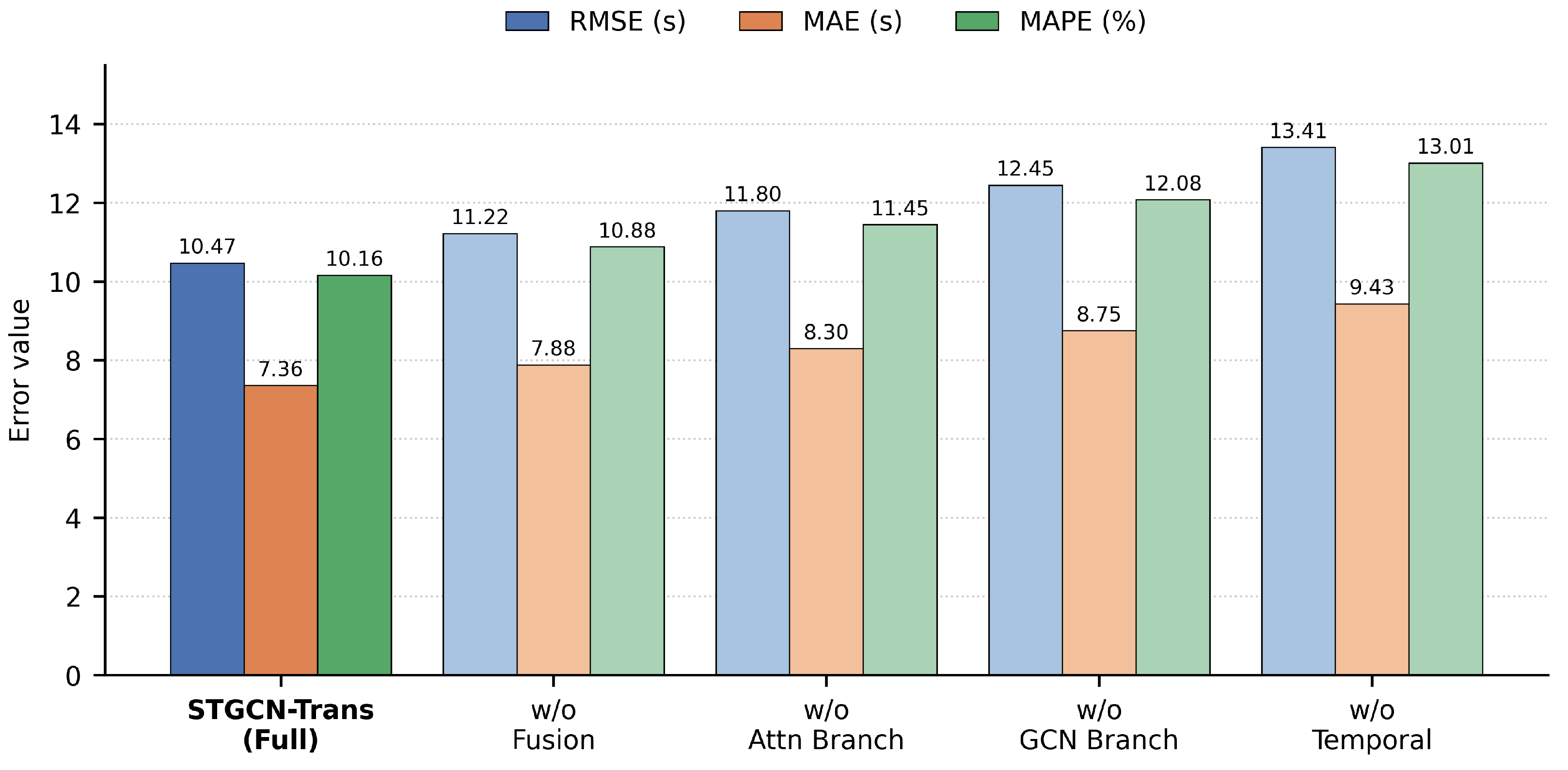
To present the performance degradation and contribution weight of each component after its removal more intuitively, the overall performance comparison for component ablation on the outbound direction is shown in Figure 15.

The quantitative and visual comparisons reveal the weight and mechanism of each main component, ranked by performance contribution from highest to lowest as follows. (1) The temporal dependency module contributes the largest performance gain. After its removal, the inbound RMSE rises from 13.55 s to 17.30 s (a 27.7% increase) and the outbound RMSE to 13.41 s, the largest error increase among all components. This is mainly because the impulsive fluctuation of bus dwell time is essentially a high-frequency temporal abrupt change, and the global temporal self-attention network can directly capture the temporal dependence of passenger-flow spikes across input window. Without this module, the model can no longer respond effectively to sudden passenger flow or capture the tidal evolution of peak-hour demand; it is therefore the primary unit for intercepting outlier errors and accommodating impulsive fluctuations. (2) The graph-convolution branch is the main unit for spatial feature extraction. After its removal, the inbound RMSE rises to 16.00 s (an 18.1% increase) and the outbound RMSE to 12.45 s, the second-largest degradation after the temporal module. This confirms that the physical passenger-flow propagation between adjacent stops cannot be ignored: the scale of passenger gathering and dispersal at an upstream stop directly affects the boarding/alighting counts and dwell time at downstream stops. The GCN module effectively captures the spatial associations between stops and the spatial propagation of passenger flow; without this branch, the model loses its perception of upstream-downstream propagation, and its accuracy declines markedly at transfer hubs and consecutive commercial stops. (3) The spatial attention branch is key to the model’s spatial generalization. After its removal, the inbound RMSE rises to 15.19 s (a 12.1% increase) and the outbound RMSE to 11.80 s, with a quantifiable accuracy decline. This branch adaptively mines implicit passenger-flow associations between non-adjacent hubs (e.g., tidal resonance across commercial districts and coupling among cross-line transfer hubs), compensating for the graph convolution’s limitation of capturing only first-order adjacency and accommodating the complex spatial dependencies of the urban bus network. (4) The external feature fusion module reduces prediction errors caused by environmental interference. After its removal, the inbound RMSE rises to 14.52 s (a 7.2% increase) and the outbound RMSE to 11.22 s; although still better than the other variants, its accuracy is measurably lower than the full model. This confirms that multi-source external features, such as weather, time of day, holidays, and route operation schedules, supplement environmental information that trajectory data can hardly cover, further improving the model’s adaptability to complex scenarios.

Through the coordinated interaction of the temporal dependency module, graph-convolution branch, spatial attention branch, and multi-source feature fusion module, the complete STGCN-Trans effectively reduces the overall average error while maintaining prediction stability at highly heterogeneous stops. Every main component contributes positively to the performance, confirming the soundness and effectiveness of the architecture.

4.4. Computational Complexity and Hyperparameter Sensitivity

Computational Cost. To assess computational cost,

Table 8. Computational complexity of the two proposed models.

Model	Parameters	Inference Time Per Sample
DSTGCN (inter-station travel)	0.047 M	0.024 ms
STGCN-Trans (station dwell)	0.584 M	0.082 ms

Measured on the environment described in Section 4.1.1, batch size 64.

reports the parameter count and per-sample inference time of the two models. Both are lightweight, with parameter counts of 0.047 M and 0.584 M and per-sample inference times below 0.1 ms, indicating that the feature-separation design introduces limited computational overhead and is suitable for practical deployment.

Hyperparameter Sensitivity. The temporal input window was set to 6 steps, balancing the coverage of recent temporal context against model complexity and the risk of overfitting on the available data. Given the strong short-term periodicity of bus operation, a substantially longer window increases computation and the number of parameters without a guaranteed accuracy gain, whereas a shorter window may omit useful recent history. For the spatial and attention configuration, the number of attention heads and graph-convolution layers was kept small to match the moderate spatial scale of a single route (on the order of tens of nodes), so as to avoid over-parameterization.

Stability. The stability of the two models across random initializations was also examined. Each model was retrained five times with different random seeds, with all other settings unchanged. Across these runs, the coefficient of variation (the standard deviation divided by the mean) of the test-set RMSE and MAE remained below 3.5% for both models. This small dispersion shows that the reported accuracy is not sensitive to random initialization and that the improvements are stable rather than the result of a single favorable run.

4.5. Summary

Combining the results of the multi-model comparison, spatial heterogeneity analysis, and ablation study, the proposed “feature separation + dual-model customization” framework effectively adapts to the differentiated spatio-temporal characteristics of the two processes in bus operation, namely inter-station travel and station dwell, which is key to the improved prediction accuracy. For inter-station travel time, which is dominated by spatial propagation along the route, DSTGCN captures the spatio-temporal dependencies across segments through dual-branch spatial feature extraction combined with an attention-enhanced temporal network; in the experiments, the complete model maintains low errors across all segments, and every component contributes positively, confirming the soundness of the architecture. For station dwell time, which is subject to sharp passenger-flow fluctuations, STGCN-Trans combines the spatial mining of graph convolution with global temporal encoding to cope with the extreme-value disturbances induced by such fluctuations; through the joint encoding of dynamic temporal features and spatial-topological dependencies, the model achieves stable accuracy gains at both ordinary steady stops and high-variability bottleneck stops.

5. Conclusions

This paper addresses the prediction of urban bus arrival time. Bus arrival time consists of two parts, inter-station travel and station dwell, whose spatio-temporal characteristics differ markedly. The former evolves smoothly and is mainly affected by the propagation of congestion on adjacent segments, whereas the latter fluctuates sharply, being disturbed by factors such as passenger flow and weather and frequently producing sudden prolonged stops and extreme values. Most existing methods treat an entire route as a single sequence for unified modeling, which makes it difficult to accommodate these two processes and results in insufficient accuracy and stability in complex scenarios. To this end, this paper divides route-level prediction into two sub-tasks, inter-station travel and station dwell, and designs a dedicated prediction model for each.

For inter-station travel time, we construct a Dual-Branch Spatio-Temporal Graph Convolutional Network. The model extracts spatial features through two parallel branches, graph convolution and spatial self-attention, which together account for congestion propagation between adjacent segments and correlations among non-adjacent yet similar segments; an attention-enhanced temporal network then characterizes their evolution over time. For station dwell time, we design a Spatio-Temporal Graph Convolutional Network with Transformer, which builds on graph convolution to capture spatial dependencies, employs a Transformer to model global temporal patterns, and adopts a smoothing loss to suppress the influence of extreme dwell times. Evaluation on the measured data of Bus Route 3 in Hohhot shows that, for inter-station travel time, DSTGCN attains the best accuracy on every metric in both directions, with an inbound RMSE of 14.74 s, 21.7% lower than that of the second-best baseline FEN-MRMGCN, and an outbound RMSE of 12.03 s. For station dwell time, STGCN-Trans attains the lowest RMSE in both directions (13.55 s inbound and 10.47 s outbound), reducing the inbound RMSE by 6.7% relative to the second-best baseline; on this task RMSE is treated as the primary metric, since dwell time is dominated by impulsive extreme values to which RMSE is more sensitive. Ablation experiments further confirm that each component contributes positively to accuracy.

This study still has several limitations, which point to directions for future work. First, the experiments are based on only a single route in Hohhot, so the generalization of the method to other routes, cities, and road-network structures remains to be verified; this could be improved by introducing cross-route and cross-city transfer learning together with few-shot learning. Second, the GPS trajectories suffer from uneven sampling and signal loss, which limits further gains in accuracy; this issue could be mitigated by combining trajectory completion with noise-robust spatio-temporal modeling. Third, the models are trained independently for each route and therefore struggle to adapt to long-term changes in the road network and passenger demand; future work could explore online incremental updating and incorporate information such as signal timing and real-time passenger flow, extending the method to practical scheduling scenarios such as transit signal priority (TSP). In addition, an end-to-end route-level ETA evaluation that accumulates predicted travel and dwell times over all downstream stops is left for future work.

References

1. Kumar, B.A.; Singh, R.; Shaji, H.E.; Vanajakshi, L. Bus arrival time prediction: A comprehensive review. IEEE Trans. Intell. Transp. Syst. 2025, 26, 7362–7379. [Google Scholar] [CrossRef] [Scilit]
2. Ma, J.; Chan, J.; Ristanoski, G.; Rajasegarar, S.; Leckie, C. Bus travel time prediction with real-time traffic information. Transp. Res. Part C Emerg. Technol. 2019, 105, 536–549. [Google Scholar] [CrossRef] [Scilit]
3. Jiang, W.; Luo, J. Graph neural network for traffic forecasting: A survey. Expert Syst. Appl. 2022, 207, 117921. [Google Scholar] [CrossRef] [Scilit]
4. Kwesiga, D.K.; Guin, A.; Hunter, M. Analysis of bus dwell times from automated passenger count data and the impact of dwell-time variability on the performance of transit signal priority. Public Transp. 2026, 18, 311–333. [Google Scholar] [CrossRef] [Scilit]
5. Bin, Y.; Zhongzhen, Y.; Baozhen, Y. Bus arrival time prediction using support vector machines. J. Intell. Transp. Syst. 2006, 10, 151–158. [Google Scholar] [CrossRef] [Scilit]
6. Gong, J.; Liu, M.; Zhang, S. Hybrid dynamic prediction model of bus arrival time based on weighted of historical and real-time GPS data. In Proceedings of the 2013 25th Chinese Control and Decision Conference (CCDC), Guiyang, China, 25–27 May 2013; IEEE: Piscataway, NJ, USA, 2013; pp. 972–976. [Google Scholar]
7. Fan, W.; Gurmu, Z. Dynamic travel time prediction models for buses using only GPS data. Int. J. Transp. Sci. Technol. 2015, 4, 353–366. [Google Scholar] [CrossRef] [Scilit]
8. Chen, C.; Wang, H.; Yuan, F.; Jia, H.; Yao, B. Bus travel time prediction based on deep belief network with back-propagation. Neural Comput. Appl. 2020, 32, 10435–10449. [Google Scholar] [CrossRef] [Scilit]
9. Hafizi, F.; Seyedabrishami, S.; Sherafat, E. Real-time prediction of bus inter-stop travel time using deep learning approach. Transp. Res. Procedia 2025, 82, 3508–3520. [Google Scholar] [CrossRef] [Scilit]
10. Ma, J.; Chan, J.; Rajasegarar, S.; Leckie, C. Multi-attention graph neural networks for city-wide bus travel time estimation using limited data. Expert Syst. Appl. 2022, 202, 117057. [Google Scholar] [CrossRef] [Scilit]
11. Rong, Y.; Yao, J.; Liu, J.; Fang, Y.; Luo, W.; Liu, H.; Ma, J.; Dan, Z.; Lin, J.; Wu, Z.; et al. Gbtte: Graph attention network based bus travel time estimation. In Proceedings of the 32nd ACM International Conference on Information and Knowledge Management, Birmingham, UK, 21–25 October 2023; pp. 4794–4800. [Google Scholar]
12. Qiu, T.; Lam, C.T.; Liu, B.; Ng, B.K.; Yuan, X.; Im, S.K. FEN-MRMGCN: A frontend-enhanced network based on multi-relational modeling GCN for bus arrival time prediction. IEEE Access 2025, 13, 5296–5307. [Google Scholar] [CrossRef] [Scilit]
13. Yin, Z.; Wang, B.; Zhang, B.; Shen, X. Prediction intervals for bus travel time based on road segment sharing, multiple routes’ driving style similarity, and bootstrap method. Appl. Sci. 2024, 14, 2935. [Google Scholar] [CrossRef] [Scilit]
14. Zhai, X.; Shen, Y. Short-term bus passenger flow prediction based on graph diffusion convolutional recurrent neural network. Appl. Sci. 2023, 13, 4910. [Google Scholar] [CrossRef] [Scilit]
15. Kipf, T.N.; Welling, M. Semi-Supervised Classification with Graph Convolutional Networks. In Proceedings of the International Conference on Learning Representations, Toulon, France, 24–26 April 2017. [Google Scholar]
16. Yu, B.; Yin, H.; Zhu, Z. Spatio-Temporal Graph Convolutional Networks: A Deep Learning Framework for Traffic Forecasting. In Proceedings of the Twenty-Seventh International Joint Conference on Artificial Intelligence, IJCAI-18; International Joint Conferences on Artificial Intelligence Organization: Somerset, NJ, USA, 2018; pp. 3634–3640. [Google Scholar] [CrossRef] [Scilit] [PubMed]
17. Li, Y.; Yu, R.; Shahabi, C.; Liu, Y. Diffusion Convolutional Recurrent Neural Network: Data-Driven Traffic Forecasting. In Proceedings of the International Conference on Learning Representations, Vancouver, BC, Canada, 30 April–3 May 2018. [Google Scholar]
18. Wu, Z.; Pan, S.; Long, G.; Jiang, J.; Zhang, C. Graph WaveNet for Deep Spatial-Temporal Graph Modeling. In Proceedings of the Twenty-Eighth International Joint Conference on Artificial Intelligence, IJCAI-19; International Joint Conferences on Artificial Intelligence Organization: Somerset, NJ, USA, 2019; pp. 1907–1913. [Google Scholar] [CrossRef] [Scilit] [PubMed]
19. Veličković, P.; Cucurull, G.; Casanova, A.; Romero, A.; Liò, P.; Bengio, Y. Graph Attention Networks. In Proceedings of the International Conference on Learning Representations, Vancouver, BC, Canada, 30 April–3 May 2018. [Google Scholar]
20. Guo, S.; Lin, Y.; Feng, N.; Song, C.; Wan, H. Attention based spatial-temporal graph convolutional networks for traffic flow forecasting. In Proceedings of the AAAI Conference on Artificial Intelligence, Honolulu, HI, USA, 27 January–1 February 2019; Volume 33, pp. 922–929. [Google Scholar]
21. Zheng, C.; Fan, X.; Wang, C.; Qi, J. Gman: A graph multi-attention network for traffic prediction. In Proceedings of the AAAI Conference on Artificial Intelligence, New York, NY, USA, 7–12 February 2020; Volume 34, pp. 1234–1241. [Google Scholar]
22. Chang, Z.; Liu, C.; Jia, J. STA-GCN: Spatial-temporal self-attention graph convolutional networks for traffic-flow prediction. Appl. Sci. 2023, 13, 6796. [Google Scholar] [CrossRef] [Scilit]
23. Vaswani, A.; Shazeer, N.; Parmar, N.; Uszkoreit, J.; Jones, L.; Gomez, A.N.; Kaiser, Ł.; Polosukhin, I. Attention is all you need. Adv. Neural Inf. Process. Syst. 2017, 30. Available online: https://papers.nips.cc/paper_files/paper/2017/hash/3f5ee243547dee91fbd053c1c4a845aa-Abstract.html (accessed on 31 August 2026).
24. Wu, H.; Xu, J.; Wang, J.; Long, M. Autoformer: Decomposition transformers with auto-correlation for long-term series forecasting. Adv. Neural Inf. Process. Syst. 2021, 34, 22419–22430. [Google Scholar]
25. Geng, Z.; Xu, J.; Wu, R.; Zhao, C.; Wang, J.; Li, Y.; Zhang, C. STGAFormer: Spatial–temporal gated attention transformer based graph neural network for traffic flow forecasting. Inf. Fusion 2024, 105, 102228. [Google Scholar] [CrossRef] [Scilit]
26. Li, Z.; Xu, H.; Gao, X.; Wang, Z.; Xu, W. Fusion attention mechanism bidirectional LSTM for short-term traffic flow prediction. J. Intell. Transp. Syst. 2024, 28, 511–524. [Google Scholar] [CrossRef] [Scilit]
27. Yu, C.; Chong, Y.W.; Budi, A.S.; Setiawan, E.; Keoh, S.L. Bus Arrival Time Prediction Using Hybrid LightGBM-LSTM. In Proceedings of the 2024 International Conference on Platform Technology and Service (PlatCon), Jeju, Republic of Korea, 26–28 August 2024; IEEE: Piscataway, NJ, USA, 2024; pp. 44–49. [Google Scholar]
28. Jeong, S.; Oh, C.; Jeong, J. BAT-transformer: Prediction of bus arrival time with transformer encoder for smart public transportation system. Appl. Sci. 2024, 14, 9488. [Google Scholar] [CrossRef] [Scilit]
29. Li, Z. DA-RNN-based bus arrival time prediction model. Int. J. Intell. Transp. Syst. Res. 2024, 22, 660–674. [Google Scholar] [CrossRef] [Scilit]
30. Lu, Y.; Wu, J.; Guo, L. Bus Arrival Time Prediction Based on the GTO-CNN-BiLSTM Model. Inn. Mong. Highw. Transp. 2023, 50–57. (In Chinese) [Google Scholar] [CrossRef]
Figure 1. Overall framework of the proposed bus arrival time prediction method.
Applsci 16 08764 g001
Figure 2. Architecture of the DSTGCN dual-branch spatio-temporal graph convolutional network.
Applsci 16 08764 g002
Figure 3. Overall architecture of the STGCN-Trans model.
Applsci 16 08764 g003
Figure 4. Summary of overall performance indicators of multi-models for bus section travel time prediction in the inbound. The red arrow indicates the RMSE reduction of DSTGCN relative to the second-best baseline (FEN-MRMGCN).
Applsci 16 08764 g004
Figure 5. Comparison of prediction accuracy of all sections in the inbound (DSTGCN vs. suboptimal FEN-MRMGCN).
Applsci 16 08764 g005
Figure 6. Comparison of prediction accuracy of all sections in outbound (DSTGCN vs. suboptimal FEN-MRMGCN).
Applsci 16 08764 g006
Figure 7. Comparison of RMSE indicators of multi-models for typical sections in the inbound.
Applsci 16 08764 g007
Figure 8. Overall performance comparison of component ablation of DSTGCN in the inbound. The dark bars denote the complete DSTGCN model, and the light bars denote the ablation variants.
Applsci 16 08764 g008
Figure 9. Comparison of RMSE distribution of each ablation variant in all sections of inbound direction.
Applsci 16 08764 g009
Figure 10. Comparison of RMSE distribution of each ablation variant in all sections of outbound direction.
Applsci 16 08764 g010
Figure 11. Summary of overall performance indicators of multi-models for bus stop dwell time prediction in the inbound direction. The red arrow indicates the RMSE reduction of STGCN-Trans relative to the second-best baseline (FEN-MRMGCN).
Applsci 16 08764 g011
Figure 12. Heatmap of the RMSE improvement rate of STGCN-Trans over four baselines at all stops: (a) uplink and (b) downlink. Warmer colours indicate larger improvements.
Applsci 16 08764 g012
Figure 13. Dumbbell chart of the absolute RMSE reduction of STGCN-Trans relative to FEN-MRMGCN at each stop, for both the inbound and outbound directions.
Applsci 16 08764 g013
Figure 14. Spatial prediction error evolution law of the core model along the stops and its baseline advantage verification.
Applsci 16 08764 g014
Figure 15. Overall performance comparison of component ablation of STGCN-Trans in the outbound directions. The dark bars denote the complete STGCN-Trans model, and the light bars denote the ablation variants.
Applsci 16 08764 g015