A Dual-Layer Aggregation Graph Neural Network for Rapid Indoor Pollutant Dispersion Prediction

Featured Application

This work can be used for emergency response to indoor pollutant dispersion. It can be applied in scenes such as chemical plants, laboratories, underground spaces, subway stations, and warehouse buildings to rapidly predict the diffusion process after a toxic gas leak, assisting in personnel evacuation, hazardous area delineation, and emergency ventilation control, enabling real-time decision-making faster than conventional numerical simulations.

Abstract

Rapid urbanization and the increasing proportion of time spent indoors have intensified concerns regarding indoor air quality and public health. Fast and reliable prediction of indoor pollutant dispersion is essential for building design optimization and risk-informed emergency response. To enable efficient indoor pollutant dispersion prediction, this study proposes a graph neural network framework with dual-layer aggregation and graph augmentation to address several limitations of traditional GNNs, including restricted receptive fields, inefficient long-range information propagation, and limited ability to capture long-range dependencies. Graph data augmentation is employed to enrich the diversity of concentration field distributions, while a dual-layer aggregation mechanism is introduced to expand the receptive field and enhance message-passing efficiency. Specifically, node features are first aggregated from adjacent edges to capture local information and are then further aggregated across nodes to incorporate global contextual features, enabling the modeling of long-range physical dependencies. Validation across multiple building configurations demonstrates that the proposed model effectively captures physical characteristics of pollutant dispersion in distant rooms and accurately predicts toxic gas dispersion under different layouts, achieving a coefficient of determination $R^2$ of up to 0.97, while delivering computational speeds approximately one order of magnitude faster than conventional CFD solvers.

1. Introduction

Rapid urbanization and the continuous expansion of urban infrastructure have fundamentally reshaped human activity patterns, with individuals spending an increasing proportion of their time indoors. Surveys indicate that urban residents typically spend 70–90% of their daily time in indoor environments [1]. As cities become denser and building functions more diversified, indoor spaces such as transportation hubs, commercial complexes, educational facilities, and industrial buildings are exposed to increasingly complex sources of airborne pollutants. Accidental releases of hazardous gases in enclosed environments such as chemical facilities, underground transport systems, and large public buildings pose substantial risks to public health and urban safety. Ensuring rapid assessment and effective response to indoor pollutant dispersion has therefore become a critical component of sustainable and resilient urban development.

Recent policy initiatives, such as the 2024–2025 Action Plan for Energy Conservation and Carbon Reduction [2], further emphasize the integration of green building strategies with intelligent environmental management. Within this context, accurate and efficient prediction of indoor airflow and pollutant transport is essential not only for routine ventilation design but also for emergency evacuation planning and risk mitigation. High-fidelity modeling tools that balance accuracy and computational efficiency are urgently needed to support real-time decision-making in smart buildings and future cities.

Computational fluid dynamics (CFD) is one of the most widely used approaches for simulating indoor pollutant dispersion [3]. By numerically solving the flow field governed by the Navier–Stokes equations and the pollutant concentration field governed by convection–diffusion equations, CFD can provide detailed and accurate distributions of indoor pollutant concentrations. Depending on the turbulence modeling strategy, CFD methods can be categorized into direct numerical simulation (DNS), Reynolds-averaged Navier–Stokes (RANS) models, and large eddy simulation (LES), among which RANS is most commonly adopted due to its balance between accuracy and computational efficiency. Numerous studies have employed CFD to evaluate pollutant distributions in air. Castellini et al. [4] conducted transient CFD simulations of the spatiotemporal dispersion of exhaled contaminants in a meeting room and identified optimal locations and configurations of air purifiers for reducing average exposure. Mohamadi et al. [5] systematically reviewed the applications of CFD during the COVID-19 pandemic, including aerosol transmission, ventilation effects, and the evaluation of protective measures. He et al. [6] investigated, using CFD, the effectiveness of air curtains in preventing airborne pollutants from entering cleanrooms. Although CFD methods [7,8] demonstrate strong applicability and high predictive accuracy in indoor environmental studies, their substantial computational cost and time consumption in resolving detailed flow fields [9] limit their suitability for real-time emergency response scenes.

To overcome the efficiency bottlenecks of conventional CFD, researchers have proposed various acceleration strategies [10], including fast fluid dynamics (FFD), state-space fluid dynamics (SFD), and Markov chain methods. Refs. [11,12,13] developed FFD approaches to solve the Navier–Stokes equations in a CFD-like manner, and Dai et al. [14] applied a dynamic Smagorinsky-based FFD method to investigate outdoor airflow and pollutant dispersion. However, because FFD relies on low-order schemes to reduce computational cost, it often suffers from reduced accuracy and excessive numerical dissipation, particularly in predicting strongly turbulent, separated, and reattaching flows. Wang et al. [15] employed state-space fluid dynamics to reconstruct governing equations using linear systems, achieving accuracy comparable to traditional CFD on structured grids with substantially reduced computational time, but its limited adaptability to unstructured grids restricts its application in complex building geometries. Although Markov chain methods can facilitate rapid pollutant dispersion prediction [16], they capture probabilistic transition patterns driven by flow fields rather than the flow fields themselves, and thus still require a series of CFD simulations in advance. Despite improvements in computational efficiency over traditional CFD, these approaches remain fundamentally based on iterative solutions of partial differential equations (PDEs), and their computational cost continues to constrain applications in dynamic leakage scenes.

Against this backdrop, the rapid development of deep learning has driven transformative changes in CFD modeling, with growing efforts to replace conventional numerical solvers using data-driven approaches [17]. Wang and Zhang [18] developed an attention-based convolutional neural network (CNN) trained on LES datasets to accurately predict high-resolution urban air quality. Jurado et al. [19] employed a multiresolution U-Net architecture to predict local pollutant dispersion in urban areas, achieving results within tens of seconds—two orders of magnitude faster than CFD while meeting established air quality modeling performance criteria. For structured-grid data, CNNs and their variants are widely adopted for flow field modeling. However, these studies rely on matrix representations of CFD outputs to accommodate CNN inputs, and the complex geometries of indoor environments fundamentally challenge this paradigm. Fixed receptive fields in structured grids limit the ability to capture long-range dependencies, hindering the identification of critical spatial features [20]. Moreover, walls, doors, and windows inside buildings form unstructured spatial layouts; in multi-zone and multi-channel indoor environments, complex boundaries induce highly nonlinear airflow patterns that strongly affect pollutant distributions. In such cases, models based on regular grids often suffer from spatial information loss, leading to degraded prediction accuracy. These limitations have motivated a shift toward deep learning frameworks designed for unstructured meshes.

Graph neural networks (GNNs), which operate directly on graph-structured data, are naturally suited to unstructured meshes and thus provide a new paradigm for indoor pollutant dispersion prediction. Shao et al. [21] developed a GNN-based model for transient toxic gas dispersion in urban environments, enabling rapid outdoor pollutant prediction driven by unstructured CFD data. However, conventional GNNs propagate information through single-layer aggregation over local neighborhoods, making it difficult to capture complex spatial dependencies in indoor environments. Zhang et al. [22] incorporated attention mechanisms to adaptively adjust spatial correlations among nodes, thereby capturing spatial characteristics of gas dispersion. To further mitigate error accumulation, Han et al. [23] introduced Transformer-based temporal attention mechanisms to model long-range dependencies, enabling stable autoregressive prediction of complex physical dynamics. Although these studies improved the limited receptive field and long-range dependency modeling of GNNs, significant challenges remain. For instance, when airflow propagates from corridors into adjacent rooms, narrow doorways induce sharp velocity variations, and the limited message-passing range of conventional GNNs with fixed-hop neighborhoods often fails to capture the turbulent features at such critical locations, leading to ineffective information transmission [24,25,26,27]. Indoor flow dynamics require simultaneous modeling of macroscopic global dispersion trends and microscopic turbulent vortex structures. Single-layer aggregation mechanisms struggle to balance accuracy and efficiency, frequently resulting in either loss of fine-scale details or excessive computational complexity. In addition, most existing studies rely solely on numerically simulated data for training; due to computational constraints, training datasets are often limited in size and diversity, yielding high accuracy only in a narrow range of scenes and restricting generalization in practical engineering applications.

To address these challenges, this study proposes a dual-layer aggregation and graph augmentation graph neural network framework (Dual-layer Aggregated Graph Augmented Graph Neural Network, DAGA-GNN), aiming to overcome the limitations of limited receptive fields and inefficient message passing in traditional graph neural networks. The proposed framework enhances long-range dependency modeling and improves prediction accuracy, enabling rapid prediction of toxic gas concentration fields as an alternative to computational fluid dynamics (CFD) solvers. By introducing graph data augmentation to enrich the directional diversity of concentration field samples, the model is exposed to pollutant dispersion patterns from multiple spatial orientations, thereby improving the utilization efficiency of limited CFD-generated training data. The method has been validated under various building configurations. The proposed framework facilitates real-time indoor air quality assessment and emergency decision-making, contributing to resilient building design and sustainable urban governance.

2. Materials and Methods

2.1. DAGA-GNN Model Architecture

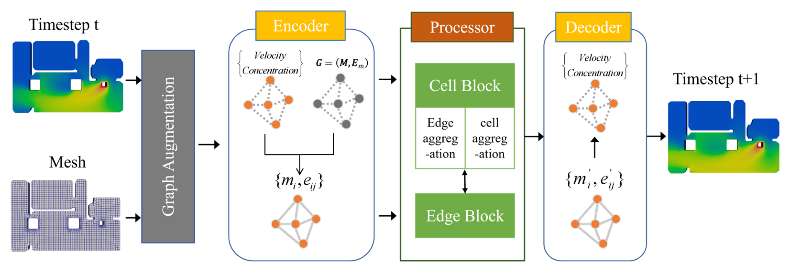
The DAGA-GNN model adopts an encoder–processor–decoder architecture to predict indoor pollutant dispersion patterns. Based on the input graph structure and concentration data, the model forecasts the flow field state at the subsequent time step. By iteratively repeating this process, the temporal evolution of indoor pollutant leakage and dispersion over a given period can be predicted. The overall framework of the proposed model is illustrated in Figure 1. This design aims to overcome the limited receptive field in capturing the coupled relationships between airflow and concentration fields and the difficulty of single-layer message passing in modeling long-range dependencies, thereby improving predictive accuracy and enabling rapid prediction of toxic gas concentration fields as an alternative to conventional CFD solvers.

The proposed model is implemented within a message-passing graph neural network framework. The CFD computational mesh is converted into a graph structure, where each mesh cell is represented as a node and adjacency relationships between neighboring cells are represented as graph edges. Physical variables associated with each cell, including velocity, pressure, concentration, and node type, are used as node features, while physical differences and geometric distances between neighboring cells are encoded as edge features. During message passing, information is exchanged along graph edges, enabling each node to aggregate local and neighboring flow information and learn the spatial interactions governing indoor airflow and pollutant transport.

2.1.1. Encoder and Decoder Modules

In graph neural networks, the encoder can be regarded as a feature extraction module that transforms raw physical variables into latent feature representations suitable for graph learning, whereas the decoder performs the inverse transformation by mapping the updated latent features back to physically meaningful quantities, including the flow and pollutant concentration fields at the next time step. In this study, the proposed model denotes the graph structure as $G=\left(\begin{array}{c}M,E_m\end{array}\right)$, where $m_i\in M$ represents cell elements and $e_{ij}\in E_m$ denotes edge attributes between adjacent cells.

The encoding stage is responsible for transforming the cell-centered graph into a higher-level feature representation to facilitate subsequent message passing and prediction. The encoder consists of a node attribute encoder $f_m$ and an edge attribute encoder $f_e$. The node encoder $f_m$ takes as input the node features $C_i$ at the current time step on the cell-centered graph, which include physical information at the cell centers, such as node type, velocity, pressure, and concentration. It outputs a 128-dimensional hidden representation $c^{\prime }$. The edge encoder $f_e$ takes as input the physical differences between adjacent cells and their coordinate offsets, which can be expressed as in Equation (1), and outputs a 128-dimensional edge feature $e_{ij}^{\prime }$. Both encoders are implemented using two linear layers with ReLU activation, followed by LayerNorm for output normalization.

$$E_{M_{ij}}=\left(u_i-u_j,c_i-c_j,\parallel x_i-x_j\parallel \right),$$

(1)

$$m^{\prime }=f_c\left(M\right),e_{ij}^{\prime }=f_e\left(E_{M_{ij}}\right),$$

(2)

The decoder module adopts a multilayer perceptron architecture similar to that of the encoder and is responsible for mapping the updated node and edge features obtained after message passing to outputs of the target dimensionality $p_i$. The output features can be interpreted as higher-order derivatives of $q_i$. By concatenating multiple output features and applying forward Euler integration with a fixed time step $∆t$, the dynamic state at the next time step $q_i^{t+1}=p_i+q_i^t$ is computed, thereby generating the mesh $M^{t+1}$ at the subsequent time instant. Each iteration of the encoder–processor–decoder framework can be regarded as producing one temporal frame in the numerical solution process, and repeated iterations yield the full spatiotemporal evolution of the domain.

2.1.2. Dual-Layer Aggregation Mechanism

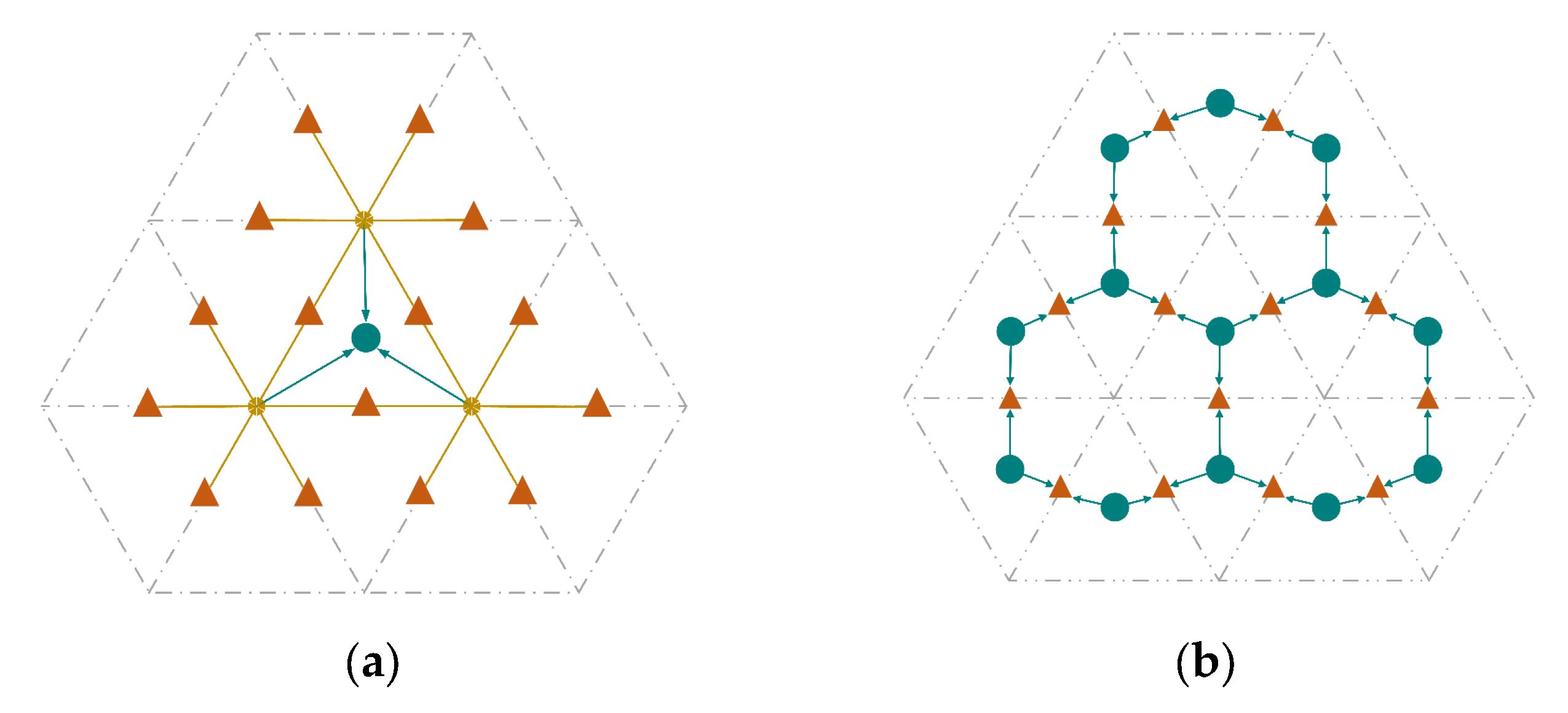
In the indoor pollutant dispersion prediction task, the processor consists of multiple message-passing layers, each comprising a cell block and an edge block, which together form the core components of the graph network. The cell block aggregates features from adjacent edges to their shared vertices, and information from multiple vertices belonging to the same cell is further fused at the cell center to update cell features. The edge block concatenates cell features with neighboring edge features and updates the edge representations accordingly. This process is illustrated in Figure 2.

During message aggregation, the model performs a dual-layer aggregation operation. First, the first-layer aggregation is conducted using Equation (3), in which features from adjacent edges are aggregated to their shared vertices, achieving an initial integration of vertex features. Subsequently, the function $f^{mp}$ aggregates vertex features within the same cell to the cell center, enabling vertex feature fusion while establishing the basis for subsequent edge-block concatenation. Afterward, neighboring cell features are fused with edge features and updated through $f^{ep}$. The overall process is formulated as follows:

$${\overline{v}}_i^{\prime }\leftarrow {\displaystyle \frac{1}{N}}(\sum e_{ij}^{\prime }),$$

(3)

$${\overline{m}}_i^{\prime }\leftarrow f^{mp}\left(m^{\prime },{\sum }_{\nu \in cell} {\overline{v}}^{\prime }\right),$$

(4)

$${\overline{e}}_{ij}^{\prime }\leftarrow f^{ep}\left(e_{ij}^{\prime },{\overline{m}}_i^{\prime },{\overline{m}}_j^{\prime }\right),$$

(5)

From the overall workflow described above, the encoder first maps physical parameters such as pollutant concentration and ventilation conditions into an initial graph representation $G_m=(m_i^{\prime },e_{M_{ij}}^{\prime })$. The graph is then input into the cell block of the message-passing layer, where features of all edges sharing the same vertex are summed to produce aggregated node features ${\overline{v}}_i^{\prime }$. In the second aggregation stage, the cell block propagates all node features within the same cell to the cell center and concatenates them with the existing hidden cell features $m^{\prime }$, which are subsequently updated through $f^{mp}$. Finally, neighboring cell features are concatenated with edge features and passed through $f^{ep}$ to update the edge representations ${\overline{e}}_{ij}^{\prime }$.The hierarchical nature of this mechanism is reflected in the fact that each node first aggregates local features from its adjacent edges, after which the cell center integrates global information from its associated nodes. In this process, $f^{mp}$ plays a role analogous to convolutional kernels in convolutional neural networks, as the two-stage aggregation over the cell-centered graph substantially expands the receptive field. This enables the model to capture longer-range feature dependencies and more effectively represent the complex physical processes governing pollutant dispersion in indoor environments.

2.2. Dataset Generation

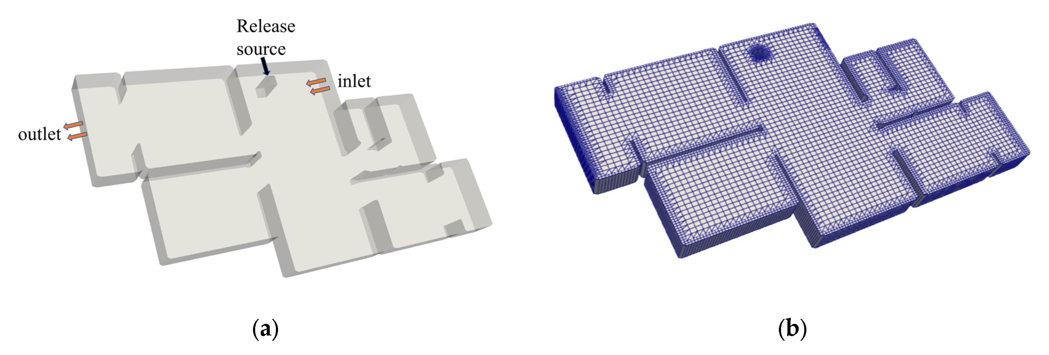
The dataset constructed in this study consists of indoor airflow velocity and pollutant concentration distributions obtained from CFD simulations of pollutant dispersion. Taking the typical indoor space model illustrated in Figure 3 as an example, the computational domain of this room is defined as a complex three-dimensional rectangle measuring 15.1 m(x) $\times$ 7.8 m(y) $\times$ 3.6 m(z) along its axes. The air inlets and outlets are represented by windows within the room: a rectangular opening on the right wall measuring 0.97 m(y) $\times$ 2.07 m(z) serves as the airflow inlet, while a rectangular opening on the left wall measuring 3.42 m(y) $\times$ 2.2 m(z) functions as the outlet. Inside the model, a 0.4 m(x) $\times$ 0.4 m(y) $\times$ 3.6 m(z) cubic region represents the pollutant release source within the building.

To construct a diverse dataset of indoor pollutant dispersion patterns, the random obstacle generation algorithm [28] was used to place obstacles and pollutant release sources at random locations within the indoor models. Inflow boundary conditions were generated using a Gaussian random number generator: inflow velocities were randomly selected within the range of 2–10 $\mathrm{m}/\mathrm{s}$, inflow angles within 45–135°, and the wind speed at the toxic gas release source was randomly selected within 2–5 $\mathrm{m}/\mathrm{s}$. These three parameters were combined to form a variety of inflow condition scenes. Based on 15 real room models, this approach was used to generate 280 distinct building models and initial condition setups. CFD simulations were conducted using the OpenFOAM platform v2212 to generate high-fidelity datasets for indoor pollutant dispersion prediction.

It should be noted that the CFD simulations in this study were conducted on a two-dimensional indoor computational domain. Most available experimental datasets for indoor airflow and pollutant dispersion are based on fully three-dimensional wind-tunnel or chamber configurations. Directly using such three-dimensional experimental data to validate the present two-dimensional simulations may introduce additional inconsistencies associated with vertical transport, wall boundary-layer effects, and three-dimensional turbulent mixing. Therefore, the CFD-generated fields in this study are not claimed to be experimentally validated measurements. Instead, they are used as numerically generated reference data for training and evaluating the proposed graph neural network-based surrogate model. To improve the reliability of the CFD-generated reference data, a series of numerical verification analyses were conducted, including mesh-sensitivity analysis, concentration contour map comparison, monitoring point concentration comparison, Courant number monitoring, solver residual assessment, and late-stage concentration variation analysis. Although these numerical verification results support the stability and mesh-resolution adequacy of the CFD simulations, the absence of direct experimental validation is acknowledged as a limitation of the present study. Future work will include tracer-gas experiments or validation against suitable two-dimensional or quasi-two-dimensional benchmark data to further assess the physical accuracy of the CFD-generated pollutant dispersion fields.

The following is a simulated implementation process. The mesh generation process was performed using the snappyHexMesh and extrudeMesh utilities in OpenFOAM v2212. The indoor geometries were initially meshed in three dimensions using snappyHexMesh to accurately capture room boundaries and internal structures. The resulting meshes were then transformed into two-dimensional computational domains through extrudeMesh by compressing the geometry along the vertical direction. This strategy significantly reduces computational complexity while retaining the dominant airflow and pollutant dispersion characteristics in the horizontal plane. The transient airflow and pollutant transport processes were simulated using the pimpleDriftFluxFoam solver under the incompressible flow assumption. This solver is based on the PIMPLE algorithm and includes the transport equation for the pollutant concentration field. Turbulence effects were modeled using the standard Reynolds-Averaged Navier–Stokes $\mathrm{R}\mathrm{A}\mathrm{N}\mathrm{S}$ $\mathrm{k}$-$\epsilon$ turbulence model. Velocity inlet boundary conditions were imposed at the ventilation openings, and no-slip conditions were applied at solid walls. For the concentration field, the pollutant concentration was defined as a normalized scalar variable. The initial concentration in the indoor domain was set to $C=0$, representing clean indoor air before pollutant release. A fixed-value concentration boundary condition of $C=1$ was imposed at the pollutant source region to represent continuous normalized pollutant release. The concentration at the ventilation inlet was set to $C=0$, indicating clean incoming air. Zero-gradient boundary conditions were employed at the outlet and solid wall boundaries for the concentration field. In the drift-flux formulation, the scalar transport equation can be expressed as:

$${\displaystyle \frac{\partial C}{\partial t}}+{\displaystyle \frac{\partial \left(U_{i}C+U_i^{\mathrm{d}\mathrm{r}\mathrm{i}\mathrm{f}\mathrm{t}}C\right)}{\partial x_i}}={\displaystyle \frac{\partial }{\partial x_i}}\left(D_{\mathrm{e}\mathrm{f}\mathrm{f}}{\displaystyle \frac{\partial C}{\partial x_i}}\right),$$

(6)

where $C$ is the normalized pollutant concentration, $t$ is time, $x_i$ denotes the spatial coordinate in the i-th direction, $U_i$ is the airflow velocity component, $U_i^{\mathrm{d}\mathrm{r}\mathrm{i}\mathrm{f}\mathrm{t}}$ is the drift velocity component, and $D_{\mathrm{e}\mathrm{f}\mathrm{f}}$ is the effective scalar diffusivity. The second term on the left-hand side represents pollutant transport by both airflow advection and drift flux, while the term on the right-hand side represents diffusion driven by the concentration gradient.

The effective scalar diffusivity was defined as:

$$D_{eff}=D_C+{\displaystyle \frac{{\nu }_t}{S{c}_t}} ,$$

(7)

where $D_C$ is the molecular diffusion coefficient of the pollutant, ${\nu }_t$ is the turbulent kinematic viscosity obtained from the $\mathrm{k}$-$\epsilon$ turbulence model, and $S{c}_t$ is the turbulent Schmidt number. The scalar transport parameters were specified in the transportProperties file. In the present simulations, the air density was set to $\rho =1.2 \mathrm{k}\mathrm{g}/{\mathrm{m}}^3$, the kinematic viscosity of air was $\nu =1.5\times {10}^{-5} {\mathrm{m}}^2/\mathrm{s}$, the molecular diffusion coefficient was $D_C=0$ and the turbulent Schmidt number was $S{c}_t=0.3$. The pollutant was modeled as a gas-phase passive scalar by setting the particle diameter to $d_p=1\times {10}^{-30} \mathrm{m}$, so that particle inertia, gravitational settling and drift effects were negligible. Therefore, under the present setting, pollutant dispersion was mainly governed by airflow advection and turbulence-induced diffusion. An adaptive time-stepping strategy was adopted in the transient simulations. The initial time step was set to 0.001 s, while the maximum allowable time step was limited to 0.01 s. The time step was automatically adjusted according to the Courant-number constraint, with the maximum Courant number set to 1. To examine the temporal stability of the numerical setup, a representative indoor scene was selected for verification. During the simulation, the monitored Courant number remained within the prescribed limit, with a mean value of approximately 0.0498 and a maximum value of approximately 0.9487. This indicates that the numerical stability requirement was satisfied under the present mesh resolution and flow conditions.

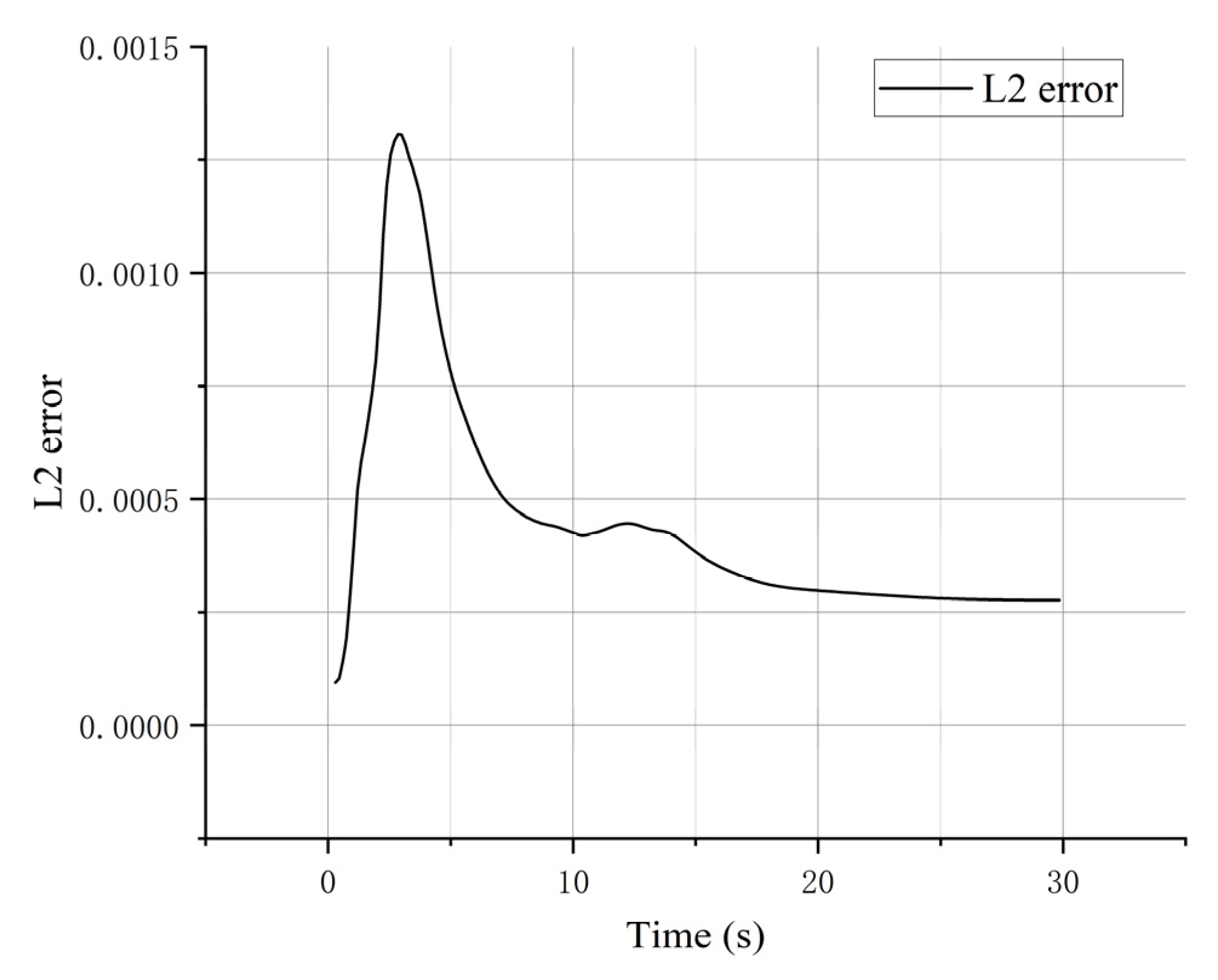
To further verify the adequacy of the selected simulation duration, pollutant concentrations at five representative monitoring points in the representative scene were compared between 25 s and 30 s. As shown in

Table 1. Comparison of pollutant concentrations at representative monitoring points in a representative indoor scene between 25 s and 30 s.

Point	25 s	30 s
Point 1	0.675	0.675
Point 2	0.315	0.316
Point 3	0.199	0.200
Point 4	0.260	0.260
Point 5	0.263	0.265

, the average relative concentration change was only 0.41%, and the maximum change was 0.97%, indicating that the concentration field had approached a quasi-steady state and that the main pollutant dispersion process had been sufficiently captured in the examined case.

In addition, to further examine the numerical stability and convergence behavior of the transient CFD simulation, solver residuals and Courant numbers were monitored in a representative indoor scene. During the initial start-up stage, the time step was automatically adjusted by the solver. After this initial adjustment, the Courant number remained stable, with the maximum Courant number at representative time instants remaining below 1. As shown in

Table 2. Solver residuals and Courant numbers at representative time instants in the pimpleDriftFluxFoam simulation.

Time/s	Max Co	U Residual	p Residual	k Residual	ε Residual	C Residual
5	0.9454	1.33 × 10−6	9.05 × 10−8	2.08 × 10−7	1.03 × 10−7	6.26 × 10−7
10	0.9486	1.34 × 10−6	8.82 × 10−8	3.31 × 10−8	5.64 × 10−8	2.02 × 10−7
20	0.9483	1.31 × 10−6	8.71 × 10−8	7.42 × 10−8	9.98 × 10−6	9.51 × 10−8
25	0.9488	1.31 × 10−6	8.63 × 10−8	5.28 × 10−8	9.98 × 10−6	1.06 × 10−7
30	0.9487	1.30 × 10−6	8.61 × 10−8	8.60 × 10−8	9.88 × 10−6	8.71 × 10−8

, the final residuals of the velocity components, pressure, turbulence quantities, and pollutant concentration equation remained at low levels during the transient simulation. At the later stage of the simulation, the final residuals of U, p, k, ε, and C were generally on the order of 10⁻⁶–10⁻⁸, except for ε, which remained around 10⁻⁵. The continuity errors also remained small, indicating that the transient calculation was numerically stable and that no divergence occurred.

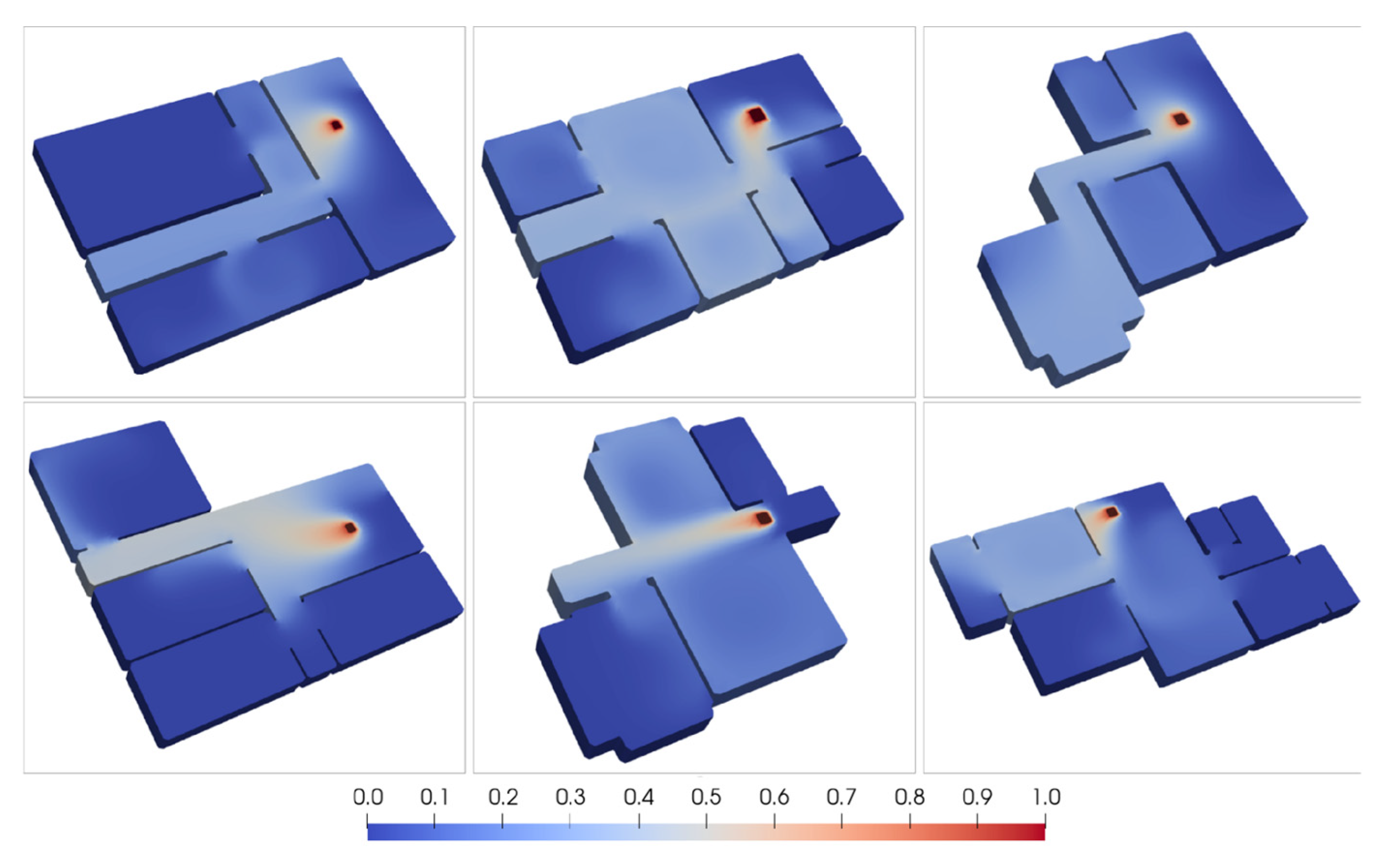
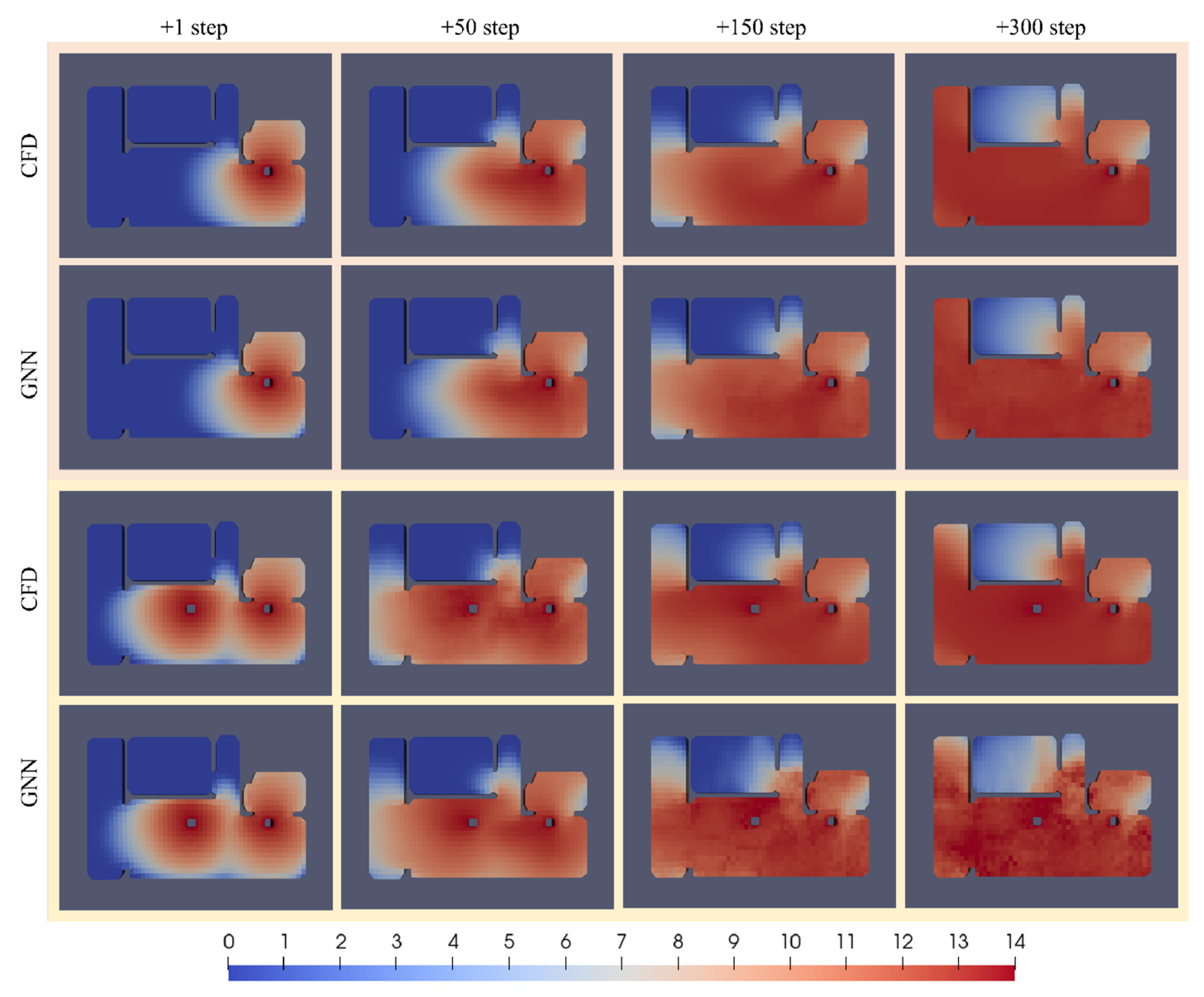
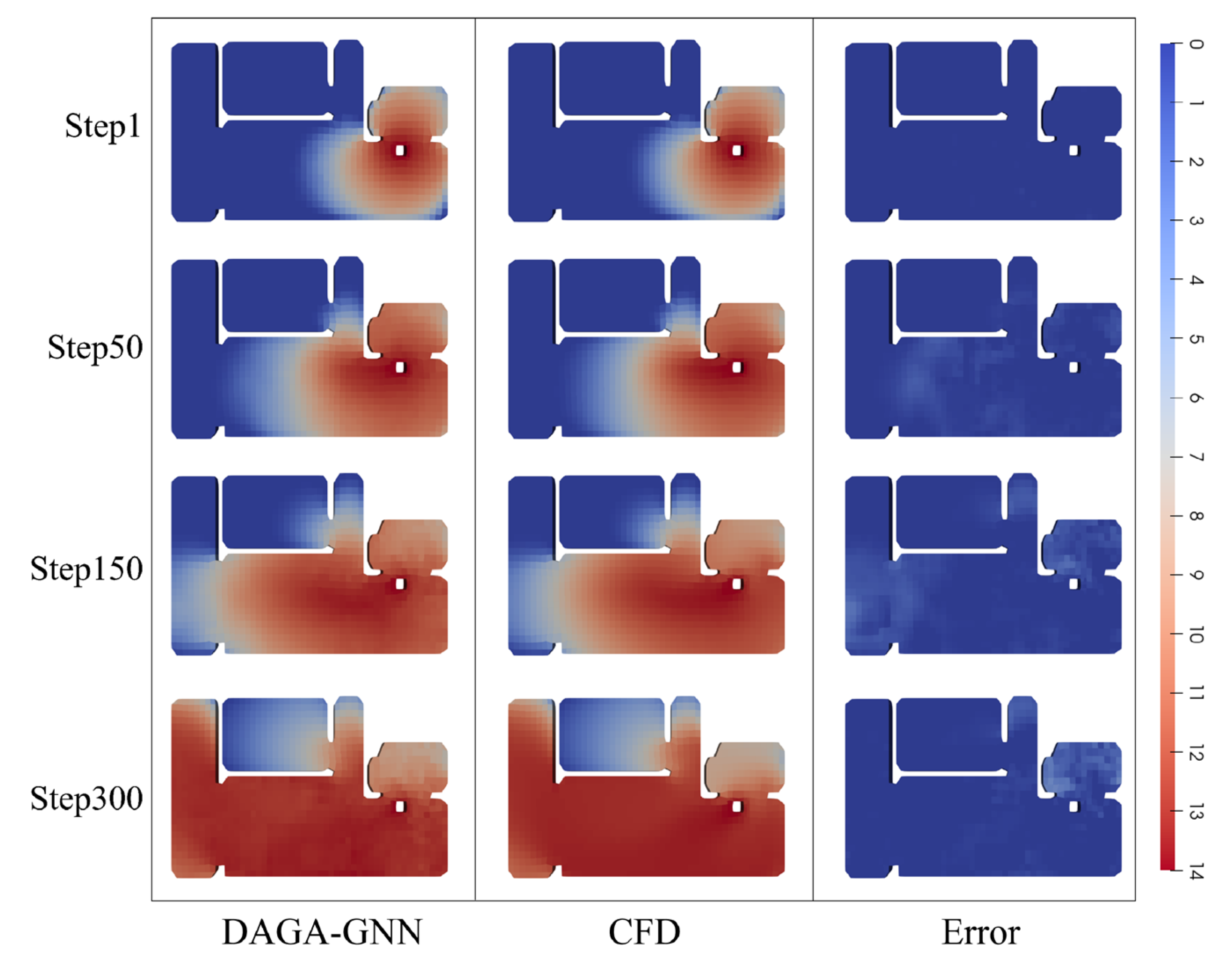
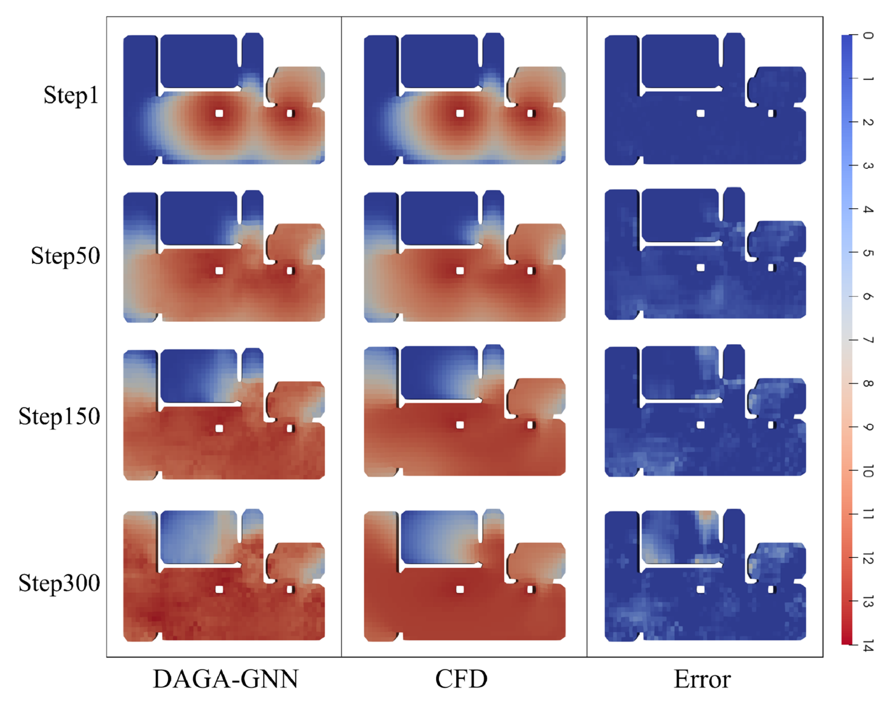
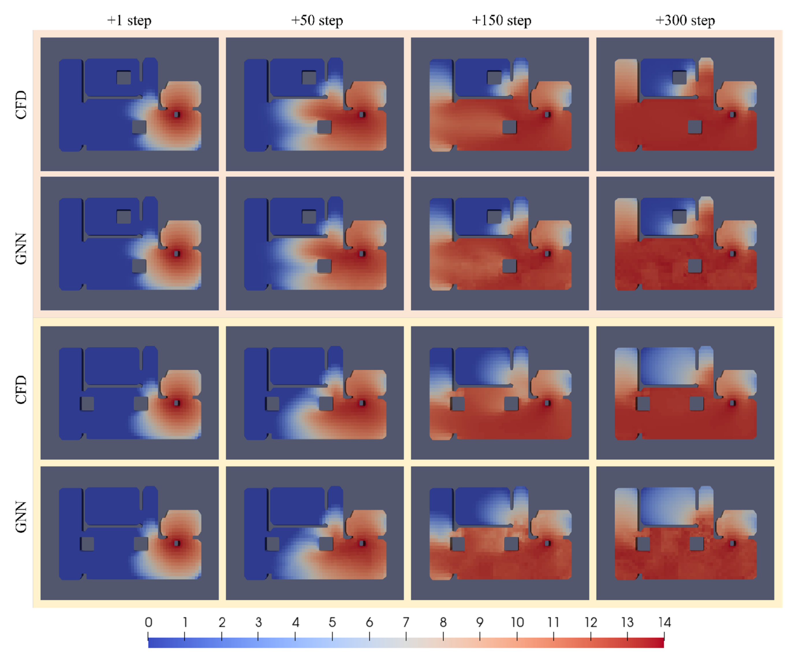
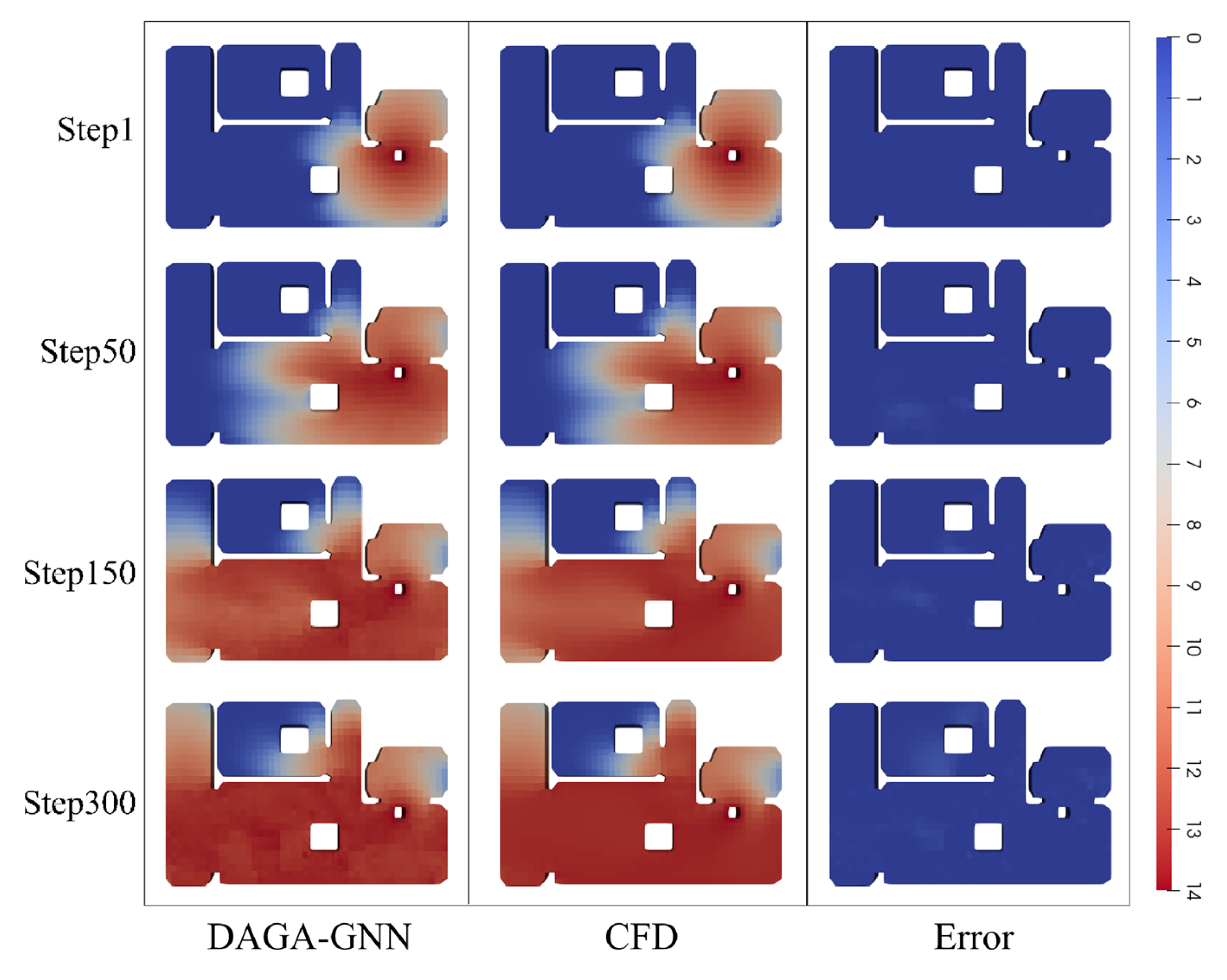
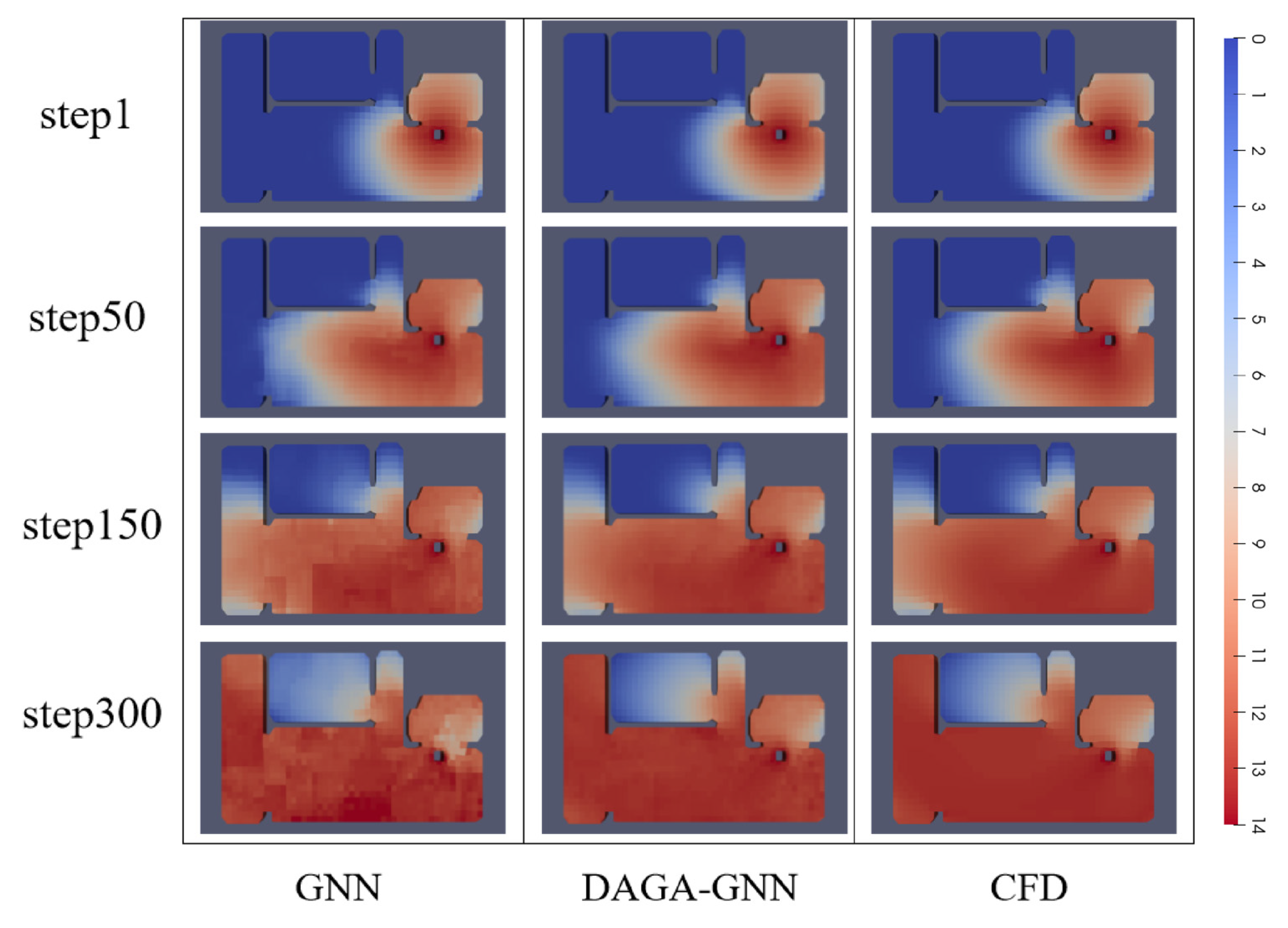
As shown in Figure 4, under the influence of room layout and initial airflow conditions, the concentration fields of toxic gas released from the source exhibit diverse distribution patterns after a period of dispersion. By varying model topologies, release source locations, initial wind speeds, and other parameters, a large and diverse set of indoor pollutant concentration data samples was generated, providing a robust dataset for subsequent model training. Selected results of pollutant dispersion simulations in the dataset are shown in Figure 4.

2.2.1. Mesh Sensitivity Analysis

To ensure that the CFD-generated pollutant concentration dataset is numerically reliable and not excessively influenced by mesh resolution, mesh sensitivity analysis was conducted using a representative indoor scene.

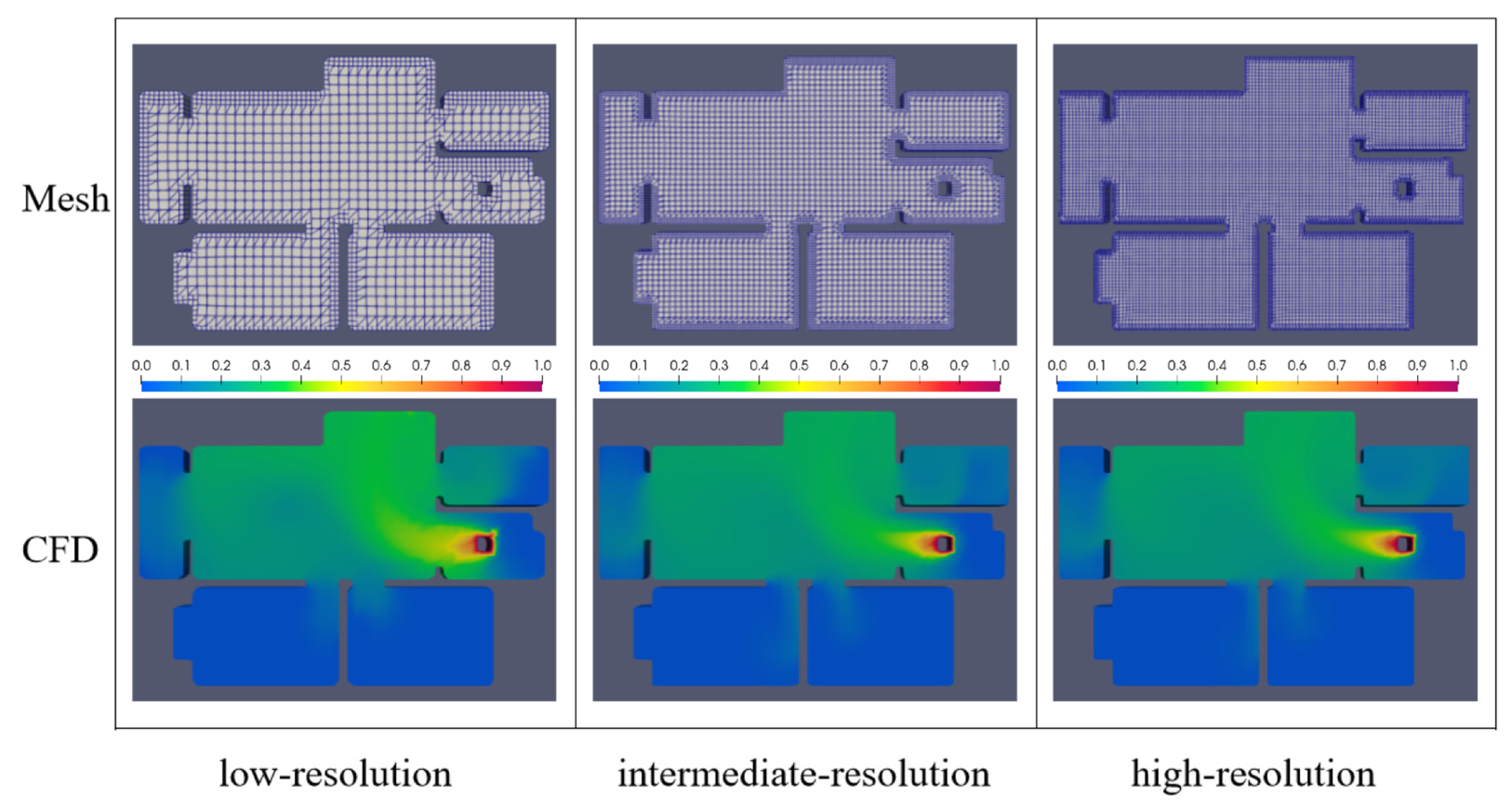
Three meshes with different resolutions were generated using the same meshing strategy, containing 2481, 6762, and 13,787 cells, respectively, as shown in Figure 5. Since the present simulations were performed on a two-dimensional indoor computational domain, the representative grid refinement ratio was estimated based on the square root of the cell-number ratio. The refinement ratios from the low-resolution mesh to the intermediate-resolution mesh and from the intermediate-resolution mesh to the high-resolution mesh were approximately 1.65 and 1.43, respectively, indicating a clear increase in mesh resolution among the three cases. The intermediate-resolution mesh was employed for dataset generation, while the low-resolution and high-resolution meshes were used to evaluate the sensitivity of pollutant dispersion predictions to mesh refinement.

Figure 5 illustrates the corresponding pollutant concentration distributions obtained using the three mesh resolutions. The low-resolution mesh exhibits noticeable discrepancies in regions characterized by strong concentration gradients, particularly near the pollutant source and along the primary transport pathway. In contrast, the concentration fields predicted by the intermediate-resolution and high-resolution meshes display highly similar spatial distributions throughout the computational domain, with only minor differences observed in localized regions. These results indicate that the intermediate-resolution mesh is capable of capturing the dominant pollutant transport characteristics with satisfactory accuracy.

To further quantify the effect of mesh refinement, pollutant concentrations at five representative monitoring points were compared among the three mesh resolutions, as shown in

Table 3. Pollutant concentration at representative monitoring points under different mesh resolutions.

Point	Low-Resolution	Intermediate-Resolution	High-Resolution
Point 1	0.6625	0.6943	0.7175
Point 2	0.3762	0.3223	0.3293
Point 3	0.2403	0.2444	0.2458
Point 4	0.3118	0.2645	0.2578
Point 5	0.3198	0.2896	0.2873

. The comparison shows that the change from the low-resolution mesh to the intermediate-resolution mesh was more pronounced than that from the intermediate-resolution mesh to the high-resolution mesh. This decreasing sensitivity with mesh refinement suggests that the numerical solution was approaching a mesh-independent trend. Although local differences still existed at individual monitoring points due to strong concentration gradients and recirculation effects, the overall pollutant dispersion pattern and the monitored concentration values became stable after the intermediate mesh resolution. Taking the high-resolution mesh as the reference, the relative differences between the intermediate-resolution and high-resolution meshes at the five monitoring points were 3.24%, 2.13%, 0.58%, 2.60%, and 0.82%, respectively. The average relative difference was approximately 1.87%, and the maximum relative difference was 3.24%. These results indicate that further refinement from 6762 to 13,787 cells had only a limited influence on the monitored pollutant concentrations and the dominant concentration distribution.

Considering the balance between numerical accuracy and computational efficiency, the intermediate-resolution mesh was selected for CFD dataset generation in this study. The results demonstrate that the adopted mesh resolution provides sufficient accuracy for predicting indoor pollutant dispersion while avoiding the significantly increased computational cost associated with further mesh refinement.

2.2.2. Graph Augmentation

In deep learning-driven fluid dynamics modeling, the training process requires large-scale datasets to capture the inherent patterns and features of the data. Small datasets can easily lead to model overfitting, while generating high-precision CFD simulation data is computationally expensive. To address this, the present study employs a graph-based data augmentation framework to jointly enhance the mesh structure, concentration fields, and airflow fields, thereby enriching the pollutant concentration dataset [29].

In the task of predicting indoor pollutant dispersion patterns, the input data consist of three key physical fields: the computational domain’s mesh structure $\mathbf{v}=(x,y{)}^T\in {\mathbb{R}}^2$, the velocity vector field $\mathbf{u}={\left(u_x,u_y\right)}^T\in {\mathbb{R}}^2$, and the pollutant concentration scalar field $c\in \mathbb{R}$. In this study, a multi-field collaborative augmentation algorithm is developed based on the rotation group SO(2) to ensure covariance of all physical fields under rotation. The rotation matrix $R_{\theta }$ is parameterized by a single angle $\theta \in \left[\mathrm{0,2}\pi \right)$, with the mesh structure, velocity field, and concentration field transformed to ${\mathbf{v}}^{\prime }=\mathbf{R}\left(\theta \right)\cdot \mathsf{\nu }$, ${\mathbf{u}}^{\prime }=\mathbf{R}\left(\theta \right)\cdot$u, and $c^{\prime }=c$, respectively.

$$R_{\theta }=\left[\begin{array}{cc}\cos \theta & -\sin \theta \\ \sin \theta & \cos \theta \end{array}\right],$$

(8)

$$\left[\begin{array}{c}{x}^{\prime }\\ y^{\prime }\end{array}\right]=\left[\begin{array}{cc}\cos \theta & -\sin \theta \\ \sin \theta & \cos \theta \end{array}\right]\left[\begin{array}{c}x\\ y\end{array}\right],$$

(9)

$$\left[\begin{array}{c}{u}_x^{\prime }\\ u_y^{\prime }\end{array}\right]=\left[\begin{array}{cc}\cos \theta & -\sin \theta \\ \sin \theta & \cos \theta \end{array}\right]\left[\begin{array}{c}{u}_x\\ u_y\end{array}\right],$$

(10)

Through this module, the input graph-structured data are randomly rotated by different angles before being fed into the model. These rotation-transformed data serve as entirely new and diverse inputs for the neural network, enabling it to learn richer and more generalizable feature representations. It should be noted that the proposed SO(2)-based augmentation does not generate new physical flow states. Instead, it leverages the rotational covariance of the governing equations to provide alternative geometric representations of existing solutions. The method assumes incompressible indoor airflow and passive scalar transport without buoyancy, thermal stratification, or other direction-dependent body forces. Under these assumptions, rotating the entire computational domain together with the associated velocity field, pollutant source location, and boundary-condition configuration yields a physically equivalent problem. Therefore, the augmented samples remain physically consistent while increasing the directional diversity of the training data. By employing this graph-based data augmentation strategy, the model can learn pollutant transport patterns from multiple spatial orientations and improve its robustness under different dispersion pathways.

2.2.3. Data Preprocessing

The network model is highly sensitive to its input data; directly feeding raw time-series data into the model can adversely affect its ability to learn the physical features of the flow field under fluid-solid coupling. Therefore, it is necessary to preprocess the input time-series airflow velocity and pollutant concentration distributions before feeding them into the model, making them more suitable for capturing the distribution characteristics of the input vectors by the GNN.

For preprocessing the pollutant concentration field, a thresholding operation is first applied to constrain the data within the [0, 1] range, eliminating extreme or anomalous values. This is followed by a linear scaling step, in which a proportional coefficient adjusts the data magnitude. Finally, a logarithmic transformation, as expressed in Equation (11), is applied, forming a combined preprocessing strategy. This composite transformation effectively smooths the data distribution while reducing variance, achieving the intended preprocessing objectives.

$$C_{norm}=\mathrm{l}\mathrm{n}\left(C\times {10}^5+1\right),$$

(11)

For the velocity field data and the preprocessed concentration field data, Z-score normalization is applied to standardize the airflow data. This normalization method subtracts the mean of the dataset from each data point and then divides by the standard deviation, resulting in data that follow a standard normal distribution. By mapping data of different scales and distributions into the same numerical space, this approach unifies the magnitude of disparate datasets, which helps improve model convergence speed and prediction accuracy. The procedure can be expressed mathematically as follows:

$${\phi }_{norm}=(\phi -{\phi }_{mean})/{\phi }_{std},$$

(12)

where $\phi$ denotes the input data, ${\phi }_{mean}$ is the mean of the dataset, ${\phi }_{std}$ is the standard deviation of the dataset, and ${\phi }_{norm}$ represents the normalized data after Z-score standardization.

2.3. Experimental Design

The DAGA-GNN model performs four rounds of message passing, and its MLP modules consist of three fully connected layers with ReLU activation functions between layers, followed by LayerNorm for final output normalization. During network training, 80% of the dataset is randomly selected as the training set, while 20% is reserved as the test set, ensuring that test data do not appear in the training set. Model weights are updated using the Adam optimizer [30], with an initial learning rate of 1 × 10⁻⁴ exponentially decaying to 1 × 10⁻⁶. Random noise is added to the input data to improve the model’s robustness to perturbations. The training loss function is the L2 loss, which is computed as the sum of squared differences between the predicted values $Z_i$ and the ground truth values ${\widehat{Z}}_i$. Mathematically, the L2 loss is defined as follows:

$$loss={\displaystyle \frac{1}{N}}{\displaystyle {\sum }_{i=1}^N} (Z_i-{\widehat{Z}}_i{)}^2.$$

(13)

To evaluate the predictive performance of the network and facilitate comparison with CFD methods, this study employs Normalized Mean Square Error (NMSE) and the correlation coefficient $R^2$ as the model accuracy metrics. The formulas for these two evaluation indicators are as follows:

$$NMSE={\displaystyle \frac{\left[{\left(O-P\right)}^2\right]}{\left[O\left]\right[P\right]}},$$

(14)

$$R^2=1-{\displaystyle \frac{\sum _i{\left(P_i-O_i\right)}^2}{\sum _i{\left(P_i-\left[O\right]\right)}^2}},$$

(15)

where $P_i$ and $O_i$ denote the predicted and true values at each node, respectively, while $\left[O\right]$ and $\left[P\right]$ represent the mean of all true values and predicted values. The correlation coefficient $R^2$ ranges from 0 to 1, with a value of 1.0 indicating perfect agreement between predictions and ground truth. The NMSE metric ranges from 0 to infinity, with smaller NMSE values indicating better predictive performance of the model.

The final loss function is defined as the sum of the individual loss terms computed separately for the velocity field and the concentration field. The specific formulation is as follows:

$$loss=\alpha \times los{s}_v+\beta \times los{s}_c,$$

(16)

where $los{s}_{\nu }$ and $los{s}_c$ denote the loss functions for the velocity field and the concentration field, respectively, while $\alpha$ and $\beta$ are the weighting coefficients for the airflow and concentration losses. During the initial training phase, $\alpha$ is set to 1 and $\beta$ to 0.3, emphasizing the model’s ability to learn the airflow field. This strategy is based on the physical dependency of pollutant dispersion on the velocity field, as accurate airflow prediction is a prerequisite for reliable concentration forecasting. Once the velocity field prediction accuracy exceeds 0.5, both $\alpha$ and $\beta$ are set to 1 to achieve balanced optimization between airflow and toxic gas concentration fields. During training, if convergence of a particular physical quantity lags, its corresponding weight can be increased to strengthen the learning of that aspect.

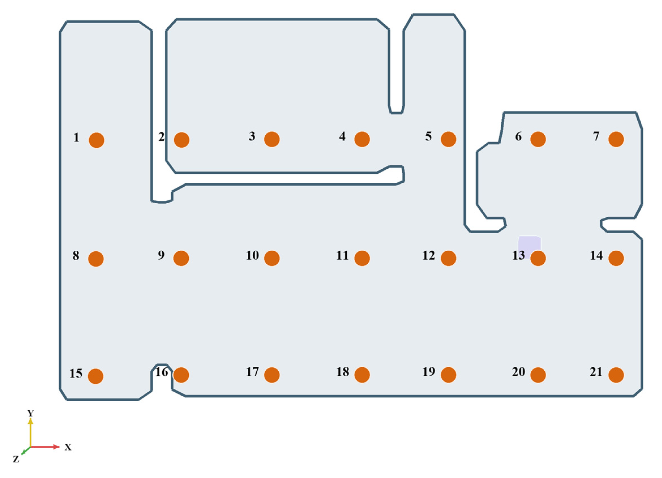
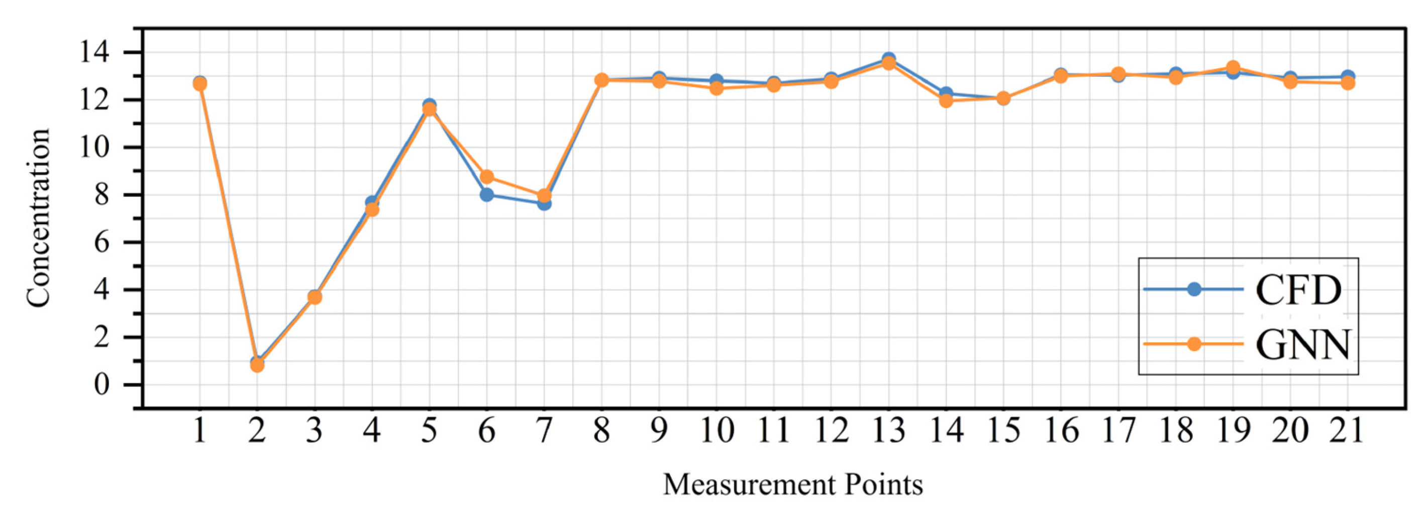
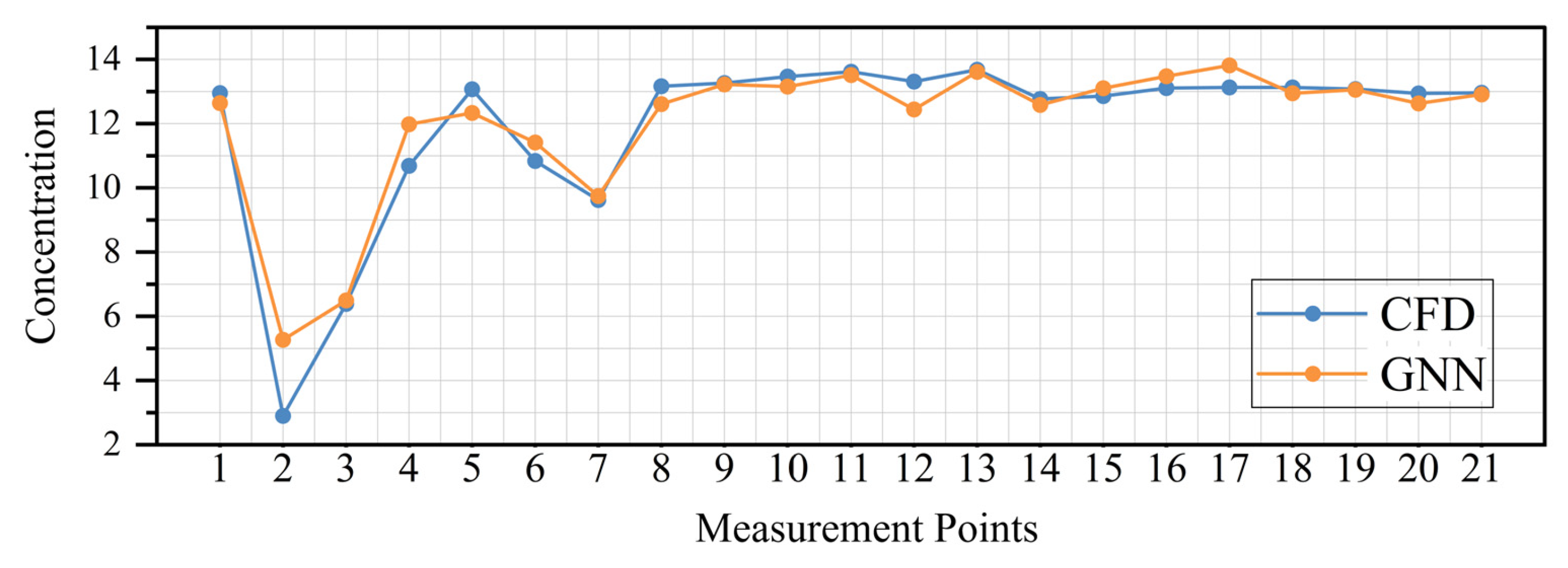
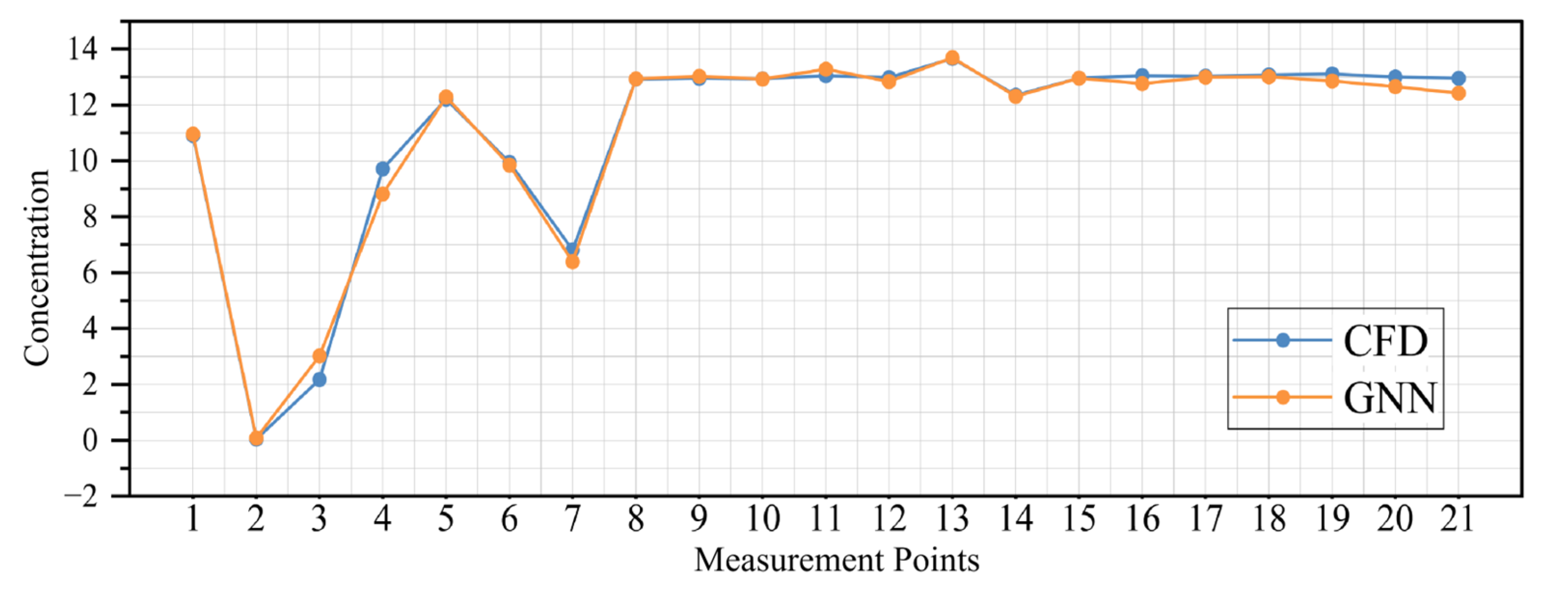
To quantitatively compare the predictions of the network model with CFD simulation results, several measurement points were placed within the experimental scene to monitor pollutant concentrations. The spatial distribution of these measurement points is illustrated in Figure 6.

3. Results

This section presents the predictions of indoor toxic gas dispersion patterns obtained using the GNN model across different experimental scenes, and provides a comparative analysis of accuracy and computational speed against the corresponding CFD simulation results.

3.1. Model Prediction Accuracy Evaluation

The comparison of GNN predictions with CFD simulation results across different scenes is shown in the contour maps in Figure 7, illustrating frames 1, 50, 150, and 300 at a breathing height of 1.6 m. The comparison demonstrates that the proposed neural network model effectively captures the flow dynamics throughout the computational domain. The predicted pollutant concentration fields are continuous and smooth, accurately reflecting the obstruction effects of room boundaries on the airflow. The model successfully predicts the generation, transport, and dissipation of vortex structures, and is capable of capturing subtle concentration variations in confined regions, such as narrow areas near door frames, indicating its strong predictive ability for the concentration field. However, discrepancies between the model predictions and CFD results still exist in certain local regions. Furthermore, the predictive performance of the model varies across different scenes, reflecting the influence of room layout and boundary conditions on its effectiveness.

To evaluate long-term prediction stability, the temporal evolution of L2 error was analyzed over the entire 30 s prediction horizon. L2 error was calculated at each time step as:

$$L2 error={\displaystyle \frac{\sum _i{(C_{pred,i}-C_{gt,i})}^2}{{\sum }_i{C_{gt,i}}^2}},$$

(17)

where i is the number of grids, while $C_{pred,i}$ and $C_{gt,i}$ represent the predicted and actual concentration values at time t, respectively. As shown in Figure 8, the error initially increases during the early transient stage when pollutant release and plume development generate strong concentration gradients. Subsequently, the L2 error decreases and gradually converges to a stable level of approximately 2.7 × 10⁻⁴. No continuous error growth or numerical divergence is observed throughout the autoregressive rollout, indicating that the proposed DAGA-GNN framework maintains stable prediction performance over the investigated prediction horizon.

To further analyze the model’s performance across different scenes, a frame-by-frame evaluation was conducted. Figure 9 presents the network model’s predictions, CFD-simulated pollutant dispersion, and the corresponding error maps at frames 1, 50, 150, and 300 for a single pollutant release source scene. From the error maps, it can be observed that the model accurately captures the trajectory of the toxic gas during the initial stages. As time progresses, larger errors appear near the pollutant release boundaries, where concentrations change rapidly and vortex structures gradually become more complex. In the later stages, as the flow field approaches steady state, the overall error decreases. However, at the junctions between the release source and the inflow boundary, error values tend to increase. These localized deviations are caused by continuous interactions between the airflow and the pollutant source, leading to cumulative error growth from initial discrepancies. Overall, the model demonstrates the ability to maintain physical conservation of the flow field while achieving the level of predictive accuracy required for engineering applications.

To further quantify the prediction results, pollutant concentrations at the measurement points in the final frame were extracted and compared with the corresponding CFD simulation results. Figure 10 illustrates the comparison of predicted and simulated pollutant concentrations at different measurement points for the current scene. Quantitative analysis shows that the mean absolute error between the two sets of results is 0.184, with over 71% of the measurement points exhibiting local errors below this average, indicating that the model achieves satisfactory predictive performance across most regions of the room. Although certain local areas, such as measurement point 6, show notable deviations with an error of 0.749, these discrepancies remain within acceptable limits for engineering applications. Overall, both the spatial distribution and the trend of the prediction curves exhibit strong agreement between the network model and CFD simulations. To further validate model performance, an evaluation metric system was constructed across multiple scenes in the training dataset. Statistical analysis indicates that the overall NMSE for pollutant concentration predictions remains at 0.323, while the correlation coefficient $R^2$ reaches up to 0.92. The complete results of all quantitative metrics are summarized in

Table 4. Evaluation metrics for predicted pollutant concentration fields for a single indoor release source.

Region	R2	NMSE
Measurement Point	0.96	0.125
Overall Region	0.95	0.323

.

Figure 11 presents the predictions of the network model, the CFD-simulated pollutant dispersion, and the corresponding error maps at frames 1, 50, 150, and 300 for a multi-source pollutant release scene. From the visualization, it can be observed that the proposed GNN model is still able to capture the hydrodynamic features across the entire concentration field and accurately predict the blocking effects of room boundaries on pollutant transport, demonstrating its capability to forecast indoor pollutant concentration fields. At the same time, discrepancies between the model predictions and CFD results are still evident in certain details. The error maps show that predictions in the early frames are relatively accurate, correctly capturing the overall direction of pollutant dispersion and performing well in regions with large airflow variations, such as near door frames. However, as the prediction progresses to later frames, both the magnitude and spatial extent of errors increase, particularly in areas where vortex structures emerge. This is due to cumulative error propagation in the sequential prediction process, where earlier inaccuracies gradually amplify, leading to larger deviations in localized regions.

To further quantify the prediction results, pollutant concentrations at the measurement points in the final frame were extracted and compared with the corresponding CFD simulation results, as shown in Figure 12. The figure illustrates the comparison of predicted and simulated pollutant concentrations at different measurement points for the multi-source pollutant release scene. Quantitative analysis shows that the mean absolute error between the network predictions and CFD results is 0.454. Although certain local areas, such as measurement point 2, exhibit noticeable deviations with an error of 2.367, this point is located in an upper corner of the room, separated from the release source by a narrow doorframe. In such confined spaces, cumulative errors during sequential prediction can lead to reduced local accuracy. Nonetheless, the overall spatial distribution and trend of the predicted concentration curves align well with the CFD results, demonstrating the model’s ability to capture the general behavior of pollutant dispersion. An evaluation metric system was constructed across multiple scenes in the training dataset, and the quantitative results of these metrics are summarized in

Table 5. Evaluation metrics for predicted pollutant concentration fields for multi-source release scene.

Region	R2	NMSE
Measurement Point	0.92	0.341
Overall Region	0.88	0.426

.

To investigate the impact of complex obstacle distributions on toxic gas dispersion in indoor airflow environments, this study employed the previously proposed random obstacle generation algorithm to construct polyhedral obstacle topologies within the computational domain, simulating typical indoor layouts such as simple furniture arrangements. Using these scene-based models, a dataset was generated to train and test the graph neural network model, which was then used to predict the corresponding toxic gas concentration distribution, resulting in dispersion contour maps.

As shown in Figure 13, the predicted concentration fields in indoor environments with obstacles are compared with CFD simulation results. The comparison demonstrates that the model effectively reproduces the dispersion patterns of toxic gas within the room, including detailed spread into smaller compartments and complex airflow phenomena around obstacles, such as flow separation and reattachment. However, as the number of prediction frames increases, relative visual discrepancies remain in regions with dense vortex structures. This is attributed to the model’s autoregressive prediction mechanism, where the output at each time step serves as input for the next, causing local errors to accumulate over time. Quantitative evaluation indicates that in the wake regions downstream of obstacles, the correlation coefficient ${\mathrm{R}}^2$ between the predicted concentrations and CFD results exceeds 0.97. This confirms the model’s applicability under complex boundary conditions while also highlighting its limitations in capturing fine-scale local flow features. To further examine prediction errors, frame-by-frame error analysis was conducted for one of the scenes, as illustrated in Figure 14.

Figure 14 presents the network model predictions, CFD-simulated pollutant dispersion, and the corresponding error maps at frames 1, 50, 150, and 300 for the prediction task. From the visual comparison, it can be observed that the model accurately predicts concentration values during the initial frames, with minimal errors. However, as the number of frames increases, some discrepancies emerge in the wake regions formed downstream of obstacles, where airflow is obstructed by the obstacles. To further quantify the prediction results, pollutant concentrations at selected measurement points in the final frame were extracted and compared with the corresponding CFD simulation results, as shown in Figure 15.

Figure 15 presents the comparison of pollutant concentration values predicted by the network model with CFD simulation results at different measurement points in an indoor environment with obstacles. Quantitative analysis shows that the mean absolute error between the two is 0.21, a deviation level that meets engineering accuracy requirements, indicating that the model achieves satisfactory predictive performance across most areas of the room. However, in certain local regions, such as measurement points 3 and 4, relatively larger deviations are observed, with a maximum error of 0.89. Analysis in Figure 15 indicates that these points are located in relatively enclosed areas near obstacles, which increases prediction difficulty. Despite these local deviations, the overall spatial distribution and trend of the predicted concentration curves align well with the CFD results, demonstrating strong agreement between the model and simulation. To further validate model performance, an evaluation metric system was constructed across multiple scenes in the training dataset. Statistical results show that the overall flow field prediction achieves an MSE of approximately 0.068, with the R² value reaching as high as 0.97.

3.2. Prediction Speed Analysis

This section evaluates and analyzes the prediction speed of the DAGA-GNN model across different scenes, focusing on a comparison of computation time between the DAGA-GNN model and a CFD solver for flow field prediction tasks.

The DAGA-GNN model is implemented using the PyTorch version 1.12.1 with GPU acceleration. Since OpenFOAM v2212 is primarily designed for CPU-based parallel computing and currently provides limited native support for GPU acceleration in standard simulation workflows, the CFD solver employs 64 CPU cores for parallel computation. The hardware used in this study consists of an NVIDIA GeForce RTX 4090 GPU (NVIDIA Corporation, Santa Clara, CA, USA) with 24 GB of memory and an Intel Xeon E5630 CPU (Intel Corporation, Santa Clara, CA, USA). The speedup reported in this study reflects the practical computational efficiency achieved under the adopted computational environment rather than a hardware-independent benchmark.

In addition, the proposed framework requires offline CFD simulations and network training to construct the surrogate model. Although these preprocessing costs can be significant, they are incurred only once during dataset generation and model development. Once trained, the DAGA-GNN model can rapidly predict indoor pollutant concentration fields for new cases within the same application domain, providing substantial computational savings for repeated evaluations and real-time prediction tasks. This performance meets the research objective of rapid prediction of indoor airflow evolution.

Table 6. Computational time analysis of DAGA-GNN inference and CFD simulation.

Scene	CFD Time Consumption (s)	DAGA-GNN Time Consumption (s)
Scene 1	3.23	0.33
Scene 2	3.51	0.34
Scene 3	3.82	0.37
Scene 4	3.51	0.35

summarizes the prediction times for both the DAGA-GNN model and the CFD solver when simulating a 20 s evolution of the flow field across different scenes. Each scene features varying inflow conditions and obstacle layouts, creating indoor environments of differing complexity. The experimental results indicate that the DAGA-GNN model consistently achieves significantly faster prediction speeds than the CFD solver in all tested scenes. Analysis of the data in Table 6 shows that the DAGA-GNN model attains a computational speed approximately 10 times faster than CFD. The variation in speedup is mainly due to differences in the number of grid cells across scenes; as the mesh size increases, the computational cost for CFD rises substantially, whereas the GNN architecture is much less affected by grid size. This enables the DAGA-GNN model to demonstrate even greater efficiency advantages in complex scenes. In summary, the DAGA-GNN model exhibits significantly higher computational efficiency compared to traditional CFD methods, achieving nearly an order-of-magnitude improvement in speed.

3.3. Ablation Study

To investigate the contributions of graph augmentation and the dual-layer aggregation mechanism, comparative analyses were conducted based on the concentration field predictions generated by a baseline GNN with the same network depth as the proposed DAGA-GNN, the proposed DAGA-GNN, and CFD simulations.

Table 7. Quantitative performance of different models in pollutant concentration field prediction.

Model	R2	NMSE
GNN	0.88	0.39
DAGA-GNN	0.95	0.32

show that under the same number of training epochs, the proposed DAGA-GNN model achieved an R² score of 0.95 and an NMSE of 0.32, while the conventional GNN model yielded an R² of 0.88 and an NMSE of 0.39.

The graph augmentation strategy adopted in this study primarily aims to enrich the diversity of concentration field distributions available during training. Unlike conventional data augmentation approaches that introduce artificial perturbations, the proposed method exploits the rotational symmetry of the governing flow and pollutant transport equations. The mesh coordinates and velocity vectors are rotated consistently under the same SO(2) transformation, while the pollutant concentration values remain unchanged. Consequently, the augmented samples remain physically consistent and represent equivalent pollutant transport processes observed from different spatial orientations.

Although graph augmentation does not generate new physical phenomena, it substantially enriches the concentration field patterns encountered during training. Indoor pollutant dispersion is strongly affected by airflow direction, obstacle arrangement, and recirculation structures. If the training samples are limited to a small number of flow orientations, the model may primarily learn concentration evolution characteristics associated with specific transport directions. Through rotational augmentation, the same pollutant transport process can be observed from multiple spatial perspectives, enabling the network to learn concentration distribution patterns under different propagation directions without requiring additional CFD simulations. As a result, the directional diversity of the training dataset is significantly increased, improving the utilization efficiency of limited CFD data and providing a richer set of concentration transport features for model learning.

The contribution of the dual-layer aggregation mechanism can be observed directly from the prediction results shown in Figure 16. In the early diffusion stage, both the conventional GNN and DAGA-GNN produce concentration distributions that are generally consistent with CFD results, indicating that local concentration characteristics near the pollutant source can be effectively captured by both models. Since the concentration gradients are primarily confined to the vicinity of the source at this stage, local neighborhood information is sufficient for accurate prediction. However, as the pollutant plume expands and propagates throughout the room, the differences between the two models become increasingly apparent. The conventional GNN exhibits noticeable deviations from the CFD results in regions far from the source. Specifically, the predicted concentration fields show weaker spatial continuity, blurred concentration gradients, and localized prediction artifacts. These discrepancies become particularly evident in the lower-left region of the room where pollutant transport is governed by long-distance airflow advection and obstacle-induced flow redistribution. In contrast, DAGA-GNN maintains much closer agreement with the CFD simulations across all diffusion stages. The predicted concentration contours remain smoother and more continuous, and the large-scale concentration distribution patterns are reproduced more accurately. In particular, the model successfully captures the gradual concentration transition from the source region to downstream areas and preserves the overall plume morphology observed in the CFD results. The concentration distributions in remote regions of the computational domain are also significantly improved compared with those predicted by the conventional GNN.

These improvements can be attributed to the proposed dual-layer aggregation mechanism. Traditional message-passing GNNs aggregate information only from immediate neighboring nodes, causing long-range dependencies to require multiple propagation steps. As the propagation depth increases, useful information may gradually weaken due to feature attenuation or over-smoothing. In indoor pollutant dispersion problems, however, concentration distributions are strongly influenced by long-distance airflow transport processes, and the concentration at a given location may depend on airflow structures originating far from that location. The dual-layer aggregation structure addresses this limitation by performing hierarchical feature integration. The first aggregation stage focuses on extracting local flow and concentration characteristics from neighboring nodes, while the second aggregation stage further propagates and integrates information over a broader spatial range. This design effectively enlarges the receptive field of the network and strengthens the transmission of non-local flow information throughout the graph. Consequently, DAGA-GNN is able to capture long-range spatial correlations and global transport characteristics more effectively than conventional GNN architectures.

Overall, the two modules contribute to the performance improvement of DAGA-GNN from complementary perspectives. Graph augmentation enriches the directional diversity of concentration field samples and enables the model to learn concentration transport characteristics from multiple spatial orientations without requiring additional CFD simulations. Meanwhile, the dual-layer aggregation mechanism enhances long-range feature propagation and global spatial information extraction, significantly improving the prediction of concentration distributions in regions far from the pollutant source. Their combination enables DAGA-GNN to achieve concentration field predictions that are substantially closer to CFD simulations than those produced by conventional GNNs, particularly in scenarios involving complex airflow transport and long-distance pollutant dispersion.

4. Discussion

For rapid prediction of toxic gas dispersion in simulated indoor environments, this study proposes a graph neural network model based on a dual-layer message aggregation mechanism (DAGA-GNN). Based on comparisons with CFD simulations across multiple building configurations, the main findings are as follows:

• DAGA-GNN provides rapid, joint prediction of airflow and pollutant concentration fields in simulated complex indoor environments.
• Graph data augmentation enriches the diversity of concentration field representations by exposing the model to pollutant dispersion patterns from multiple spatial orientations, thereby improving the utilization efficiency of limited CFD training data.
• The dual-layer aggregation mechanism expands the effective receptive field and enhances long-range feature propagation, enabling more accurate prediction of pollutant transport and concentration distributions in simulated complex indoor environments.
• Validation in simulated indoor environments demonstrates that DAGA-GNN accurately reproduces CFD-predicted toxic gas concentration fields, achieving an R² value of up to 0.97. Compared with conventional CFD methods, the proposed framework reduces computational time by approximately one order of magnitude while maintaining high prediction accuracy.