Impact on Data Assimilation of Extended Coverage of GNSS Zenith Total Delay Network in Southern Part of the MetCoOp Domain

Abstract

Global Navigation Satellite Systems (GNSS) signals are delayed by the atmosphere, and the resulting zenith total delay (ZTD) provides valuable information on atmospheric water vapour for numerical weather prediction (NWP). Despite the demonstrated benefits of GNSS ZTD assimilation, the southern part of the Meteorological Cooperation on Operational Numerical Weather Prediction (MetCoOp) domain remains sparsely observed, particularly along the main southwesterly moisture-transport pathway into Fennoscandia. This study investigates the impact of assimilating additional ZTD observations from northern Germany—provided by the Helmholtz Centre for Geosciences (GFZ)—into the MetCoOp system. By extending ZTD coverage upstream of the forecast domain, the study addresses a documented gap in previous MetCoOp assimilation research, which has largely focused on densely observed regions or event-specific cases. Since moisture transport into Fennoscandia is climatologically dominated by southwesterly flow from the North Sea, particularly during summer, strengthening ZTD coverage in the southern MetCoOp domain therefore provides critical upstream constraints on humidity and temperature advection. Using the convection-permitting High-Resolution Limited Area Model—Applications of Research to Operations at Mesoscale (HARMONIE–AROME) model coupled with the Surface Externalisée scheme (SURFEX), two experiments were run for June–August 2025: a baseline configuration and one including GFZ ZTDs. Assimilating GFZ data significantly refines the mid-to-lower-tropospheric moisture field (500–925 hPa). Although domain-averaged differences remain modest—specific humidity variations of ~1.3 g kg⁻¹ and temperature deviations near 1 K—spatial analyses reveal sharper moisture gradients and improved boundary-layer structure over land. These findings demonstrate that enhanced upstream ZTD density provides valuable constraints on moisture advection and latent-heat-related processes, thereby improving short-range humidity analyses in a high-resolution NWP system and complementing earlier studies conducted in Fennoscandia.

1. Introduction

Global Navigation Satellite Systems (GNSS) are primarily designed for high-precision positioning, but their signals are delayed by atmospheric water vapour, temperature, and pressure. These delays, expressed as zenith total delay (ZTD), degrade positioning accuracy and simultaneously provide valuable information on atmospheric humidity, and are measured in units of metres. Through appropriate inversion techniques, GNSS offers continuous, high-temporal-resolution (~15-min) observations under nearly all weather conditions, making ZTD an important data source for numerical weather prediction (NWP). In this study, we assess the impact of assimilating GNSS-derived ZTDs in the south of Fennoscandia into the High-Resolution Limited Area Model—Applications of Research to Operations at Mesoscale (HARMONIE–AROME) [1,2], used operationally within the Meteorological Cooperation on Operational Numerical Weather Prediction (MetCoOp) system [3]. Moisture transport into Fennoscandia is climatologically dominated by southwesterly flow associated with North Atlantic cyclones and the Norwegian Sea storm track, meaning that humid air masses frequently enter the region from northern Germany and the North Sea. Because this inflow corridor is sparsely covered by operational ZTD observations, additional ZTD data from northern Germany represent a strategically important extension of the southern MetCoOp domain and may improve humidity and temperature analyses.

Numerous studies have demonstrated the value of assimilating GNSS ZTD in NWP (see e.g., [4]) with consistent improvements across a wide range of models, resolutions, and meteorological conditions. Early work using variational methods showed that ZTD assimilation enhances synoptic-scale circulations and precipitation forecasts in global and regional systems, including four-dimensional variational data assimilation (4D-VAR; [5,6]) implementation [7]. Several studies further demonstrated reductions in humidity, temperature, and geopotential-height biases when ZTDs are assimilated together with conventional observations [8,9,10,11]. In convection-permitting and high-resolution regional models, ZTD assimilation has been shown to improve the representation of water vapour, precipitation, and convective processes. Positive impacts have been reported in the Weather Research and Forecasting model [12] over Poland [13], and multiple studies have highlighted enhanced short-term forecasts during convective events [14,15,16]. Additional work using three-dimensional variational data assimilation (3D-VAR; see e.g., [17]) and nudging approaches has demonstrated improved ZTD and integrated water vapour analyses at kilometre-scale resolution [18,19]. More recent studies continue to confirm these benefits, showing reduced humidity uncertainty in the mid-to-lower troposphere and improved forecasts of temperature, wind, and specific humidity [20]. Torcasio et al. [21] demonstrated enhanced temperature, moisture, and wind analyses when assimilating 388 ZTDs over Italy. Additional high-resolution Weather Research and Forecasting model studies have shown improved water vapour fields across seasons [22], enhanced short-term precipitation skill with hourly ZTD updates [23], and substantial reductions in humidity errors when combining ground-based and airborne ZTDs [24]. Recent findings also indicate that assimilating tropospheric gradients together with ZTDs further improves humidity analyses, particularly in regions with sparse GNSS coverage [25]. However, most Fennoscandian ZTD assimilation studies have focused either on densely observed regions or on event-specific cases in regions other than the MetCoOp domain. The impact of extending ZTD coverage upstream of the MetCoOp domain is the novel idea of this study. Despite the demonstrated benefits of GNSS ZTD assimilation, the southern part of the MetCoOp system domain remains sparsely covered by operational ZTD observations, limiting the representation of moisture inflow from northern Germany into Fennoscandia. To address this gap, the present study assimilates additional ZTDs from the Helmholtz Centre for Geosciences (GFZ) network in northern Germany into the convection-permitting HARMONIE–AROME system, thereby extending observational coverage in a key upstream region for moisture and temperature advection into Fennoscandia. Two parallel experiments—one including GFZ ZTDs (GFZ-exp) and one without (CRTL-exp)—are conducted to quantify their impact on analyses and short-range forecasts of temperature, humidity, and wind. This is the first study to evaluate the influence of GFZ ZTD assimilation in the southern MetCoOp domain, providing new insight into how enhanced ZTD coverage improves moisture representation in a high-resolution NWP system.

2. Methodology

In this section, we briefly review the principle of ZTD estimation based on the carrier-phase observations, and later we explain how these ZTDs are connected to the meteorological parameters and generation of observation operators for assimilation of ZTDs based on the 3D-VAR scheme.

2.1. Estimation of ZTD from Precise Point Positioning with Ionosphere-Free Carrier Phase Observations

The purpose of this section is to provide the theoretical background for ZTD estimation, instead of describing a processing chain implemented in this study. All ZTDs assimilated in HARMONIE–AROME are taken directly from the European Meteorological Network EIG GNSS Water Vapour Programme (E-GVAP) operational product (http://egvap.dmi.dk (accessed on 26 August 2026)) stream without modification. Its analysis centres compute ZTDs using their standard precise point positioning pipelines employing a mapping function. The ZWD operator in HARMONIE–AROME uses the model’s native 65 hybrid vertical levels and spatial horizontal resolution of 2.5 km, ensuring consistency with the background humidity profile.

Generally, all GNSS transmit at least two carrier frequencies, which enables users to mitigate the ionospheric delay effect. For instance, the Global Positioning System employs the frequencies $f_1$ = 1575.42 MHz and $f_2$ = 1227.60 MHz [26]. By forming a specific linear combination of the carrier-phase measurements used for precise point positioning—known as the ionosphere-free combination—a new observation equation can be derived from Equation (1) that is independent of the ionospheric delay term. In general, the ionosphere-free carrier-phase observation (${\mathsf{\Phi }}_{\mathrm{I}\mathrm{F}}$) is used, where the subscript IF stands for the ionospheric-free term; the equation can be expressed as [26,27,28,29]

$${\mathsf{\Phi }}_{\mathrm{I}\mathrm{F}}=\rho +c\mathsf{\Delta }\delta +m\left(e\right){\mathsf{\Delta }}^{\mathrm{Z}\mathrm{T}\mathrm{D}}+N_{\mathrm{I}\mathrm{F}}\hspace{1em}\mathrm{with}\left(\begin{array}{c}{\mathsf{\Phi }}_{\mathrm{I}\mathrm{F}}\\ N_{\mathrm{I}\mathrm{F}}\end{array}\right)={\displaystyle \frac{f_1^2{\lambda }_1}{f_1^2-f_2^2}}\left(\begin{array}{c}{\mathsf{\Phi }}_1\\ N_1\end{array}\right)-{\displaystyle \frac{f_2^2{\lambda }_2}{f_1^2-f_2^2}}\left(\begin{array}{c}{\mathsf{\Phi }}_2\\ N_2\end{array}\right)$$

(1)

where c is the speed of light in a vacuum $\rho$ stands for the geometric distance between the satellite and receiver, $\mathsf{\Delta }\delta$ represents the difference between receiver and satellite clock errors, $N_{\mathrm{I}\mathrm{F}}$ stands for the ambiguity parameter for the ionospheric-free combination where $N_1$ and $N_2$ are the ambiguity parameters of the first and second signals with ${\lambda }_1$ and ${\lambda }_2$, respectively, as the signal wavelengths. m(e) is the mapping function converting slant tropospheric delay to ZTD, and e denotes the satellite elevation angle. ${\mathsf{\Phi }}_1$ and ${\mathsf{\Phi }}_2$ are the received phases of the first and second signals, respectively; note that both of them should be corrected for the satellite clock measurements prior to being used. ${\mathsf{\Delta }}^{\mathrm{Z}\mathrm{T}\mathrm{D}}$ stands for the ZTD.

Several mapping functions have been developed to model m(e), including the Niell Mapping Function [30], the Vienna Mapping Function 1 [31], and the Global Mapping Function [31]. These functions generally assume a stratified and isotropic troposphere above each GNSS station. Although m(e) depends weakly on meteorological parameters such as pressure, humidity, and temperature—typically obtained from nearby radiosondes or numerical weather model outputs—it is far more sensitive to the satellite elevation angle. Böhm et al. [31] demonstrated that Vienna Mapping Function 1 provides the best consistency with radiosonde data compared with other mapping models, which has been typically applied by the E-GVAP analysis centres.

Today, different software packages have been developed for processing GNSS data, and most of them include modules for precise point positioning and network solutions in which a mapping function is used for estimating the ZTD. For instance, the Nordic GNSS Analysis Centre (NGAA) uses the Bernese GNSS Software v5.2, developed by the Astronomical Institute of the University of Bern [32]. The Helmholtz Centre for Geosciences (GFZ) has developed its own processing system, the Earth Parameter and Orbit System [33], for precise GNSS data analysis. Other analysis centres employ GIPSY-OASIS (GPS-Inferred Positioning System and Orbit Analysis Simulation Software), developed by the Jet Propulsion Laboratory [34], or GPS Analysis at Massachusetts Institute of Technology/Global Kalman Filter [35]. In short, ZTD, although primarily a geodetic product, has become a valuable observation type for NWP. Establishing the link between ZTD and meteorological parameters and assimilating these data effectively into NWP systems, a topic discussed in the following section.

2.2. GNSS ZTD Observation Operator

The purpose of this section is to describe the theoretical formulation of the ZTD observation operator, rather than a GNSS processing chain. The assimilation of GNSS ZTDs in HARMONIE–AROME is performed through the standard variational observation operator used in the MetCoOp system. The operator computes model-equivalent ZTDs by vertically integrating the hydrostatic and wet refractivity components along the zenith direction. This operator evaluates the model’s humidity and pressure fields to produce a simulated ZTD that can be compared with the ZTD products. The hydrostatic component is derived from the model pressure field using the Saastamoinen formulation, while the wet component is obtained by integrating the model-level water-vapour. All computations use the native vertical discretisation of HARMONIE–AROME, which consists of 65 hybrid layers extending from the surface to 10 hPa. This ensures that the ZTD operator is fully consistent with the model’s vertical resolution and avoids additional interpolation. The role of the observation operator in this study is therefore limited to converting model humidity and pressure fields into model-equivalent ZTDs for use in the variational assimilation system.

The ZTD consists of a hydrostatic (dry) component, which spans the atmosphere from the tropopause to approximately 80 km, and a wet component, which is confined to the troposphere. In mid-latitude standard-atmosphere representations, the troposphere extends to about 11 km, although the actual tropopause height varies with latitude, season, and synoptic conditions [36]. Thus, the ZTD can be expressed as

$${\mathsf{\Delta }}^{\mathrm{Z}\mathrm{T}\mathrm{D}}={\mathsf{\Delta }}^{\mathrm{Z}\mathrm{H}\mathrm{D}}+{\mathsf{\Delta }}^{\mathrm{Z}\mathrm{W}\mathrm{D}}$$

(2a)

${\mathsf{\Delta }}^{\mathrm{Z}\mathrm{H}\mathrm{D}}$ stands for the zenith hydrostatic delay (ZHD) and ${\mathsf{\Delta }}^{\mathrm{Z}\mathrm{W}\mathrm{D}}$ the zenith wet delay (ZWD).

Theoretically, the ZTD has a vertical integral relationship with meteorological parameters for both the hydrostatic (ZHD) and wet (ZWD) components, extending from the station level up to the top of the troposphere. Vedel et al. [36] solved this relation numerically and compared the results with the ZHD derived from the well-known Saastamoinen [37] model. They concluded that the Saastamoinen model provides a good approximation of the ZHD and is, moreover, much simpler to implement than full numerical integration. This model is expressed as

$${\mathsf{\Delta }}^{\mathrm{Z}\mathrm{H}\mathrm{D}}=2.2768\times {10}^{-5}[\mathrm{m}/\mathrm{P}\mathrm{a}]{\displaystyle \frac{p_a}{1-2.66\times {10}^{-3}\mathrm{c}\mathrm{o}\mathrm{s}\left(2\theta \right)-2.8\times {10}^{-7}\left[{\mathrm{m}}^{-1}\right]h_a}}$$

(2b)

where $p_a$ is the atmospheric pressure at the GNSS antenna, $\theta$ and $h_a$ are, respectively, the latitude and height of the GNSS station.

The ZWD can be computed using the following formula, which represents the discrete form of the integral expression used to determine the ZWD above a GNSS station. This equation serves as the observation operator that links the ZWD to the total ZTD, and subsequently to the meteorological parameters within a NWP model.

$${\mathsf{\Delta }}^{\mathrm{Z}\mathrm{W}\mathrm{D}}={\displaystyle \frac{R}{g\left(\theta \right)}}{\sum }_{i=1}^M{q}_i\left(k^{\prime }+{\displaystyle \frac{k_3}{T_i}}\right)\left(p_{i+1/2}-p_{i-1/2}\right).$$

(2c)

According to Equation (2c), the troposphere is assumed to be stratified into M layers. Here, R denotes the gas constant for dry air, and $g\left(\theta \right)$ represents the gravitational acceleration as a function of latitude. Vedel and Huang [4] demonstrated that, due to the relatively low scale heights of humidity, the variation of g with height can be neglected when determining the ZWD. $q_i$ and $T_i$ represent the specific humidity and temperature in the i-th layer, respectively, while $p_{i+1/2}-p_{i-1/2}$ denotes the pressure difference between the upper and lower boundaries of that layer. Finally, according to Bevis et al. [38], $k^{\prime }$ = $2.21\times {10}^{-7} [\mathrm{K}/\mathrm{P}\mathrm{a}]$ and $k_3$ = $3.7\times {10}^{-3} [{\mathrm{K}}^2/\mathrm{P}\mathrm{a}]$.

Although Equation (2c) shows the standard integral expression for the wet delay, it is included only to describe the theoretical formulation of the observation operator. The operator does not apply refractivity constants such as $k_2^{\prime }$ or $k_3$; instead, it computes the wet delay directly from the model’s humidity and temperature fields. All GNSS-specific processing is performed by the analysis centres, and the ZTDs assimilated in this study are used exactly as provided.

Equations (2b) and (2c) can also be used to estimate the ZTD from meteorological parameters, providing background ZTD fields for NWP systems. The difference between ZTD values derived from GNSS measurements and those from a NWP model can serve as a tool for quality assessment and potential bias-correction; see Section 4.2.1. It is important to note that the mathematical models for ZHD and ZWD are approximations of reality. Every assumption and simplification introduces deviations from the true atmospheric state, which can result in biases in the derived products. For example, the model may have a limited height (10 hPa), and differences may exist between model orography and station height; assuming that the atmosphere around each GNSS station is stratified, homogeneous, and isotropic is not strictly realistic, but such assumptions are necessary to define mapping functions. This difference introduces additional bias (see refs. [39,40] for a bias formulation). The use of the Saastamoinen model is another source of approximation, even if it is a good one. On the other hand, GNSS observations reflect the actual state of the atmosphere, but they are subject to limitations, including measurement noise and finite sensitivity. Therefore, when assimilating ZTD data into NWP systems, it is essential to account for both the biases introduced by the mathematical models and the observational errors. Another important source of bias is the height difference between height of stations and model orography as represented by the coarser resolution at that position. In the next section, the principle of data assimilation based on the 3D-VAR method is explained briefly.

2.3. Principle of 3D-VAR and Bias-Correction

Data assimilation is a key component of NWP, serving as the link between the model and observations. It can be formulated as a sequential least-squares estimation problem, where one set of equations represents the model dynamics—in this case, the HARMONIE-AROME NWP model—and the other represents the available observations, including ZTD data. In such an estimation, the assumption of variability in both the model outputs and the observations is crucial, as even small systematic errors can strongly influence the results. Only random noise is effectively minimised through the procedure. However, since mathematical models are inherently imperfect, their outputs inevitably contain biases. Therefore, bias-correction is an essential step to mitigate systemic effects and ensure the success of the data assimilation process. Bias-correction can be implemented either statically or variationally [39,40]. In the static approach, the bias is estimated by comparing forecasted ZTDs from the model with observed ZTDs over a defined period. The variational approach, on the other hand, is more advanced and estimates the bias simultaneously with the control vector during the assimilation process [39,40]. In order to explain how the variational bias-correction method is applied in a 3D-VAR assimilation system, consider the following objective function:

$$\begin{gathered} J\left(\mathbf{x},\mathsf{\beta }\right)={\displaystyle \frac{1}{2}}{\delta \mathbf{x}}^{\mathrm{T}}{\mathbf{B}}^{-1}\delta \mathbf{x}+{\displaystyle \frac{1}{2}}{\delta \mathsf{\beta }}^{\mathrm{T}}{\mathbf{B}}_{\mathsf{\beta }}^{-1}\delta \mathsf{\beta }+ \\ +{\displaystyle \frac{1}{2}}{\left(\mathbf{y}-\underset{\_}{h}\left(\mathbf{x},\mathsf{\beta }\right)-{\mathbf{H}}_{\mathbf{x}}\delta \mathbf{x}-{\mathbf{H}}_{\mathsf{\beta }}\delta \mathsf{\beta }\right)}^{\mathrm{T}}{\mathbf{R}}^{-1}\left(\mathbf{y}-\underset{\_}{h}\left(\mathbf{x},\mathsf{\beta }\right)-{\mathbf{H}}_{\mathbf{x}}\delta \mathbf{x}-{\mathbf{H}}_{\mathsf{\beta }}\delta \mathsf{\beta }\right). \end{gathered}$$

(3a)

In fact, $\delta \mathbf{x}=\mathbf{x}-{\mathbf{x}}_{\mathrm{b}}$ and $\delta \mathsf{\beta }=\mathsf{\beta }-{\mathsf{\beta }}_{\mathrm{b}}$ where $\mathbf{x}$ is the control vector, $\mathsf{\beta }$ the vector of variational biases, and ${\mathbf{x}}_{\mathrm{b}}$ and ${\mathsf{\beta }}_{\mathrm{b}}$, respectively, the background control vector and bias, $\mathbf{B}$ and ${\mathbf{B}}_{\mathsf{\beta }}$ are, respectively, the background variance-covariance matrix of the background control variables and the background biases, respectively. $\underset{\_}{h}\left(\mathbf{x},\mathsf{\beta }\right)=h\left(\mathbf{x}\right)+b\left(\mathsf{\beta },\mathbf{x}\right)$ is the augmented observation operator $h\left(\mathbf{x}\right)$ with the bias-correction vector [39,40]:

$$b\left(\mathsf{\beta },\mathbf{x}\right)={\sum }_{j=0}^{N_p}{\beta }_j{p}_j\left(\mathbf{x}\right)$$

(3b)

where ${\beta }_j$ are the unknown biases and $p_j$ are called the predictors and $N_p$ total number of them. At present, we use one predictor as a constant offset after some sensitivity studies and tests [41] in the MetCoOp system.

Finally, ${\mathbf{H}}_{\mathbf{x}}={\displaystyle \frac{\partial \underset{\_}{h}\left(\mathbf{x},\mathsf{\beta }\right)}{\partial \mathbf{x}}}$ and ${\mathbf{H}}_{\mathsf{\beta }}={\displaystyle \frac{\partial \underset{\_}{h}\left(\mathbf{x},\mathsf{\beta }\right)}{\partial \mathsf{\beta }}}$.

The sequential 3D-VAR solution considering variational bias correction is

$$\left(\begin{array}{c}{\delta \mathbf{x}}^{\mathrm{a}}\\ {\delta \mathsf{\beta }}^{\mathrm{a}}\end{array}\right)=\left(\begin{array}{c}{\delta \mathbf{x}}^{\mathrm{b}}\\ {\delta \mathsf{\beta }}^{\mathrm{b}}\end{array}\right)+\left(\begin{array}{c}\mathbf{B}{\mathbf{H}}_{\mathbf{x}}^{\mathrm{T}}\\ {\mathbf{B}}_{\mathsf{\beta }}{\mathbf{H}}_{\mathsf{\beta }}^{\mathrm{T}}\end{array}\right){\left({\mathbf{H}}_{\mathbf{x}}\mathbf{B}{\mathbf{H}}_{\mathbf{x}}^{\mathrm{T}}+{\mathbf{H}}_{\mathsf{\beta }}{\mathbf{B}}_{\mathsf{\beta }}{\mathbf{H}}_{\mathsf{\beta }}^{\mathrm{T}}+\mathbf{R}\right)}^{-1}\left(\mathbf{y}-\underset{\_}{h}\left(\mathbf{x},\mathsf{\beta }\right)-{\mathbf{H}}_{\mathbf{x}}\delta \mathbf{x}-{\mathbf{H}}_{\mathsf{\beta }}\delta \mathsf{\beta }\right)$$

(3c)

${\delta \mathbf{x}}^{\mathrm{b}}$ and ${\delta \mathsf{\beta }}^{\mathrm{b}}$ are, respectively, variations of the background control vector and bias, ${\delta \mathbf{x}}^{\mathrm{a}}$ and ${\delta \mathsf{\beta }}^{\mathrm{a}}$ are their analysis counterparts, and the covariance matrix of the estimated parameters is

$$\mathrm{C}=\left[\mathbf{I}-\left(\begin{array}{c}\mathbf{B}{\mathbf{H}}_{\mathbf{x}}^{\mathrm{T}}\\ {\mathbf{B}}_{\mathsf{\beta }}{\mathbf{H}}_{\mathsf{\beta }}^{\mathrm{T}}\end{array}\right){\left({\mathbf{H}}_{\mathbf{x}}\mathbf{B}{\mathbf{H}}_{\mathbf{x}}^{\mathrm{T}}+{\mathbf{H}}_{\mathsf{\beta }}{\mathbf{B}}_{\mathsf{\beta }}{\mathbf{H}}_{\mathsf{\beta }}^{\mathrm{T}}+\mathbf{R}\right)}^{-1}\right]\left(\begin{array}{cc}{\mathbf{H}}_{\mathbf{x}}\mathbf{B}& {\mathbf{H}}_{\mathsf{\beta }}{\mathbf{B}}_{\mathsf{\beta }}\end{array}\right).$$

(3d)

In the cost function (3a), there are three quadratic forms, which the first one says that the estimate should be as close as possible to the background parameters, the second means that the estimated bias should be close to the background bias in the model domain, and the third one means that the transformed background by the observation and bias operators should reproduce observation as close as possible to the real observations, or in other words, minimisation in the observation domain.

The 3D-VAR formulation used in this study assumes that observation errors are unbiased, Gaussian-distributed, and horizontally uncorrelated, the latter reflected in the use of a diagonal observation-error covariance matrix R. These assumptions motivate several elements of the preprocessing and quality-control strategy. A variational bias-correction is applied to remove systematic components of the observation error and ensure consistency with the unbiased-error assumption. Since $\mathbf{R}$ is diagonal, and no horizontal or vertical error correlations are modelled for data including GNSS ZTDs, the observation error becomes an important tuning parameter that determines the relative weight of the ZTDs in the variational system. A 12 mm value as the error of ZTDs was initially derived from observation-minus-background and observation-minus-analysis departures, and subsequently adjusted to ensure a balanced influence between the observations and the background, as well as consistency with other moisture-related observations. An independent diagnostic following Desroziers et al. [42] produced similar values, supporting the choice of 12 mm. The matrix $\mathbf{B}$ is also treated as diagonal in the observation space; the underlying background-error statistics are derived from an ensemble of short-range forecasts generated from perturbed initial and boundary conditions.

A thinning distance of 50 km through an allowlist is used to reduce the impact of horizontally correlated ZTD observations, which are not represented in the diagonal R matrix and could otherwise degrade the analysis. According to Poli et al. [7], assuming that most of the ZTD information is concentrated in the lowest 3 km of the troposphere and that elevation angles in excess of 10 degrees are used, the resulting ZTD measurements represent a horizontal area of radius 17 km, centered at the station. Therefore, the distance between any two stations should be larger than 34 km to avoid correlation. The thinning distance plays a key role in maintaining statistical consistency and a 50 km thinning distance lies safely within the decorrelation scale of ZTD observation errors [7]; this threshold is therefore adopted in the present configuration.

In addition, a first-guess check is employed to screen out gross errors that would violate the Gaussian-error assumption and introduce non-linear behaviour into the cost function [11]. Together, these steps ensure that the observations entering the assimilation are consistent with the statistical assumptions underlying the 3D-VAR scheme.

2.4. The MetCoOp System and 3D-VAR

In the MetCoOp system, the non-hydrostatic, high-resolution HARMONIE-AROME model is used to produce short-range forecasts. The model explicitly resolves key physical processes—including radiation, microphysics (cloud particle formation and evolution), turbulence, and land–surface interactions—through the Surface Externalisée scheme [43]. Its fine spatial/horizontal resolution and detailed physics make it well suited for forecasting localised phenomena such as fog, heavy precipitation, and strong winds, although some biases, such as temperature errors over snow-covered and glaciated surfaces, remain the subject of ongoing research. The HARMONIE-AROME configuration used in MetCoOp is further adapted for Nordic conditions through modifications to microphysics, surface drag, and snow schemes, and it assimilates a wide range of observations—including radiosondes, satellite radiances, radar reflectivities, and GNSS-derived ZTD—to improve forecast skill in complex terrain, coastal regions, and rapidly evolving weather situations [3]. Within MetCoOp, upper-air humidity is primarily constrained by radiosonde profiles, while radar and satellite radiances provide complementary information on vertical moisture structure. GNSS ZTD contributes continuous, horizontally dense total-column water-vapour information and, unlike most other observation types, is available under all weather conditions and at high temporal resolution or measurement rates. Operational forecasting within MetCoOp also includes the MetCoOp Ensemble Prediction System, which provides ensemble forecasts on a ~2.5 km grid to quantify expected weather and associated uncertainties, and the MetCoOp Nowcasting system, which delivers very short-term, high-frequency forecasts.

Here, we discuss the implementation of the 3D-VAR scheme within this system. The computational domain has a horizontal resolution of 2.5 km and 65 vertical levels, with the lowest model level around 12 m (1030.6 hPa) above ground and the highest at 30–32 km (10 hPa). The domain forms a three-dimensional grid of cubic cells, each containing meteorological information such as temperature, humidity, and wind speed components. Forecasting is performed by the HARMONIE-AROME model across the entire 3D grid, and data assimilation is carried out to update the model state using observations. The model provides the background (or first-guess) field, which serves as prior information for the assimilation process. Here, the observations are compared with model equivalents derived from the background vectors using observation operators. Since observations are usually not located exactly at the model grid points, interpolation within these operators links the observed values to the model field. As a result, only the elements of the background vector near the observation locations are significantly updated during the analysis step. Each observation type influences the model fields primarily around its representative altitude, depending on the vertical correlation structure of the background error covariance matrix. In areas where observations are sparse or missing, the corresponding parts of the background vector receive little or no direct update, although nearby observations may influence them through spatial correlations.

In the 3D-VAR method used in the MetCoOp system, all variables in the 3D domain are analysed simultaneously by minimising a cost function that balances the differences between the background and the observations. The resulting analysis vector replaces the background and serves as the first-guess (background) field for the next assimilation cycle. This process is repeated at every cycle to continually refine the model state. Unlike Kalman filtering, 3D-VAR does not update the background error covariance matrix B from one cycle to another. However, the structure of B can change with height, since the characteristics of the short-range forecast errors vary with height. Typically, the horizontal correlation length scales are shorter in the lower atmosphere and increase with height. This is physically reasonable, as various surface inhomogeneities cause small-scale spatial variations at lower levels while the horizontal scales of variation are larger in the upper troposphere. In the HARMONIE-AROME model, the scheme proposed by Berre [44] is applied for generating B, in which the forecast error covariances are estimated with a spectral approach and from a set of forecast differences and autocovariances are calculated with a non-separable scheme, and multiple linear regressions are used in the formulation of cross covariances.

3. GNSS ZTD Processing Centres

Several European institutions provide high-quality near real-time ZTD estimates to the E-GVAP. These centres operate independent GNSS processing systems that support operational meteorology and NWP by delivering timely and reliable tropospheric products. Key contributors include Nordic GNSS Analysis Centre (NGAA), the Royal Observatory of Belgium (ROB), the United Kingdom Meteorological Office (MetOffice) and GFZ.

The NGAA processes data from approximately 700 GNSS stations across Fennoscandia and provides ZTD products. ZTDs are estimated hourly using a network solution in Bernese v5.2 [45], applying Centre for Orbit Determination in Europe orbits, the Finite Element Solution 2004 Ocean Tide Model [46], and IGS14 antenna models [47]. The Vienna Mapping Function is used as the Global Mapping Function with a 10° elevation cut-off. Although each station uses coordinates fixed from a solution 14 days earlier, the change in the height component is typically below 1 mm provided no significant motion has occurred (e.g., no earthquake) during that period. A difference of this magnitude affects the estimated ZTD by less than 0.3 mm, which is negligible for practical purposes [11].

The ROB processes GNSS observations from the European Reference Permanent Network [48], the International GNSS Service [49], and the Belgian national networks Flanders Positioning Service and Wallonia Continuously Operating Reference Stations. In total, ROB analyses data from about 720 stations to generate ZTD products. Using Bernese v5.0, ROB applies double-differenced Global Positioning System-only processing to reduce systematic errors. Its near real-time system provides 15-min ZTD estimates from roughly 380 stations with a latency below 1.5 h, while a sub-hourly system under development will run four cycles per hour using real-time data from about 180 stations. It also operates a daily post-processing chain that delivers high-accuracy coordinates and ZTDs for validation and reanalysis, reprocessed once final International GNSS Service products become available after approximately 21 days.

The GFZ is an operational water vapour programme analysis centre, processing data from more than 600 GNSS stations using the EPOS.P.V2 software [33]. It provides hourly near real-time ZTDs with a latency below 15 min, used operationally by the German Meteorological Service, the MetOffice, and Météo-France. This centre is also the only water vapour programme centre delivering high-resolution slant total delays at 2.5-min intervals. Processing follows International Earth Rotation Service standards [50], applies Pagiatakis [51] ocean loading, Niell mapping function [30], and Bevis et al. [38] for integrated water vapour conversion. Station coordinates are fixed in the International Terrestrial Reference Frame using International GNSS Service products, and Ultra-Rapid orbits (3-hourly) combined with parallel precise point positioning processing ensure delivery within 15–20 min.

The University of Luxembourg, in collaboration with the MetOffice, produces global and regional near real-time ZTD products for the water vapour programme using Bernese v5.4. Three product lines are generated: global hourly, regional hourly, and regional sub-hourly (15-min). These products are validated against the water vapour programme reference solutions, Double-Difference Network post-processing, and ECMWF Reanalysis Version 5 [52] integrated water vapour fields. The increased temporal resolution enhances NWP assimilation during rapidly evolving weather events and ensures a robust near real-time data flow.

Amongst these analysis centres GFZ is the one that uses multi-GNSS data for computing the ZTD with a cut-off angle of 7°, whilst the other mentioned centres used the Global Positioning System with cut-off angle of 10°.

4. Experiment Setup

In order to study the effect of adding the ZTDs from northern Germany, provided by GFZ, into the data assimilation process of the MetCoOp system, two experiments were conducted under identical conditions. In both experiments, conventional observations, such as synoptic, ship, and aircraft observations and radiosonde (balloon) measurements, were used, as well as satellite observations and observations from weather radars. The experiment configurations and input datasets were very similar to the operational MetCoOp runs and identical, except for the inclusion of ZTD stations. In the control experiment (CTRL-exp), ZTD data from NGAA, ROB, and the Met Office were assimilated, while in the second experiment, here and after we named it GFZ-Exp, the ZTDs provided by GFZ were additionally included. The GNSS data are also allowlisted and spatially thinned to avoid duplicated stations and overly dense coverage. Stations appearing in multiple databases are removed during merging, and a minimum spacing is applied to limit observation error correlations, which are not accounted for in the current 3D-VAR formulation, that can degrade forecast quality. In this study, a thinning distance of 50 km (see [11]) is considered.

We used ZTDs provided by the E-GVAP for the period from 15th to 31st June. The first month was allocated for the spin-up process to stabilise the model with the initial and boundary conditions, enabling it to respond accurately to any desired input spin-up process. Furthermore, the variational bias-correction coefficients are determined during this step. The ZTDs were supplied in European Cooperation in Science and Technology format at near-hourly intervals (59 and 45 min), converted to ASCII format, and subsequently merged, allowlisted, and spatially thinned to hourly resolution. Furthermore, an error of 12 mm has been chosen for the ZTDs based on diagnostic data assimilation feedback statistics. After a one-month spin-up period in June 2025, both experiments were warm-started from the same spin-up and then run through the end of August 2025, covering approximately three months with 3-hourly cycles with 12-h forecast period.

All other observation types follow the operational MetCoOp HARMONIE–AROME configuration. A complete description of the observation processing, quality-control rules, and assimilation procedures for conventional observations, satellite radiances, and radar data is provided in [3], which documents the MetCoOp system in detail. In this study, we use a model version and assimilation setup that are as close as possible to the operational configuration; therefore, the treatment of all non-GNSS observations is identical to that described in [3].

4.1. Experimental Design, Domain and Distribution of GNSS ZTD

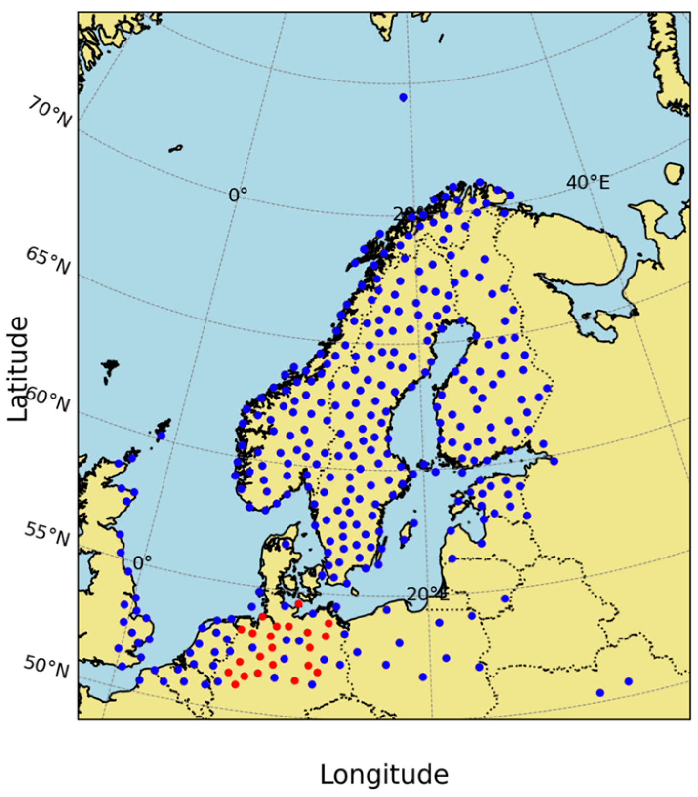
To assess the spatial distribution and coverage of the GNSS ZTD observations used in this study, the locations of the stations from the different datasets were analysed and visualised. Figure 1 illustrates the final configuration of the allowlisted and spatially thinned stations used for data assimilation over the study area. The stations common to both experiments are represented by blue circles, where the red circles indicate stations from the GFZ network. In the operational MetCoOp NWP system, the majority of the stations are processed by the NGAA. Additionally, ZTD data processed by MetOffice and the ROB in Belgium are included to add some additional stations not processed by NGAA. These three datasets are represented by small blue circles in Figure 1. The GFZ ZTDs are displayed as small red circles.

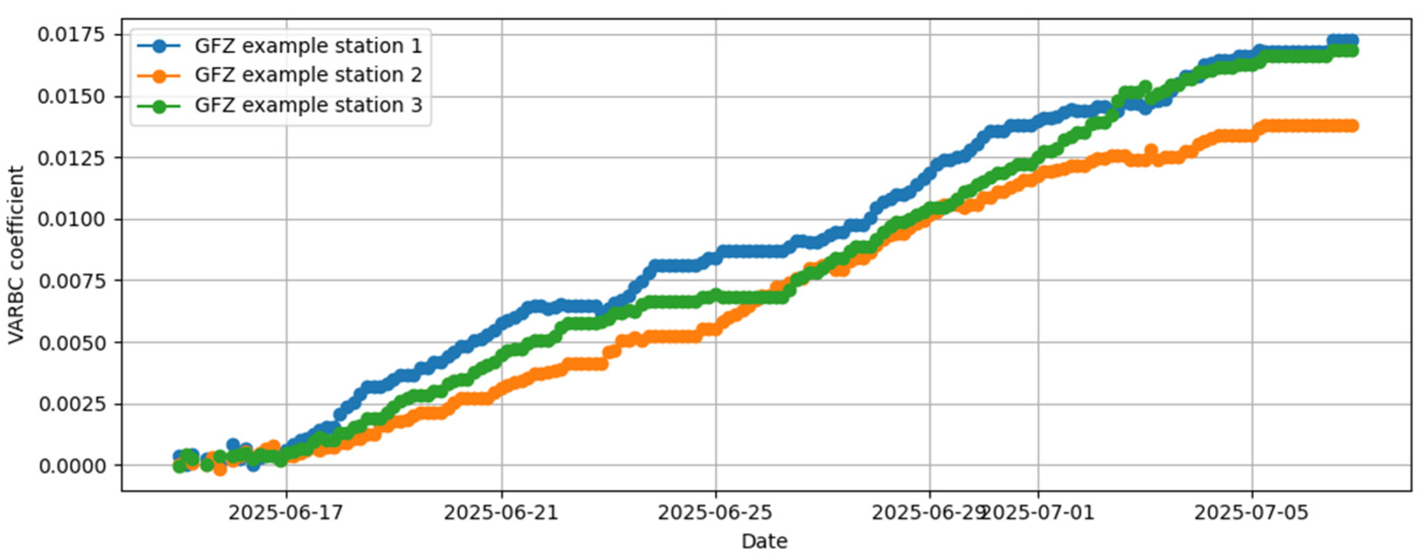
Figure 2 illustrates the spin-up of the variational bias-correction coefficients for three newly assimilated GNSS stations. The coefficients start from zero on 15 June 2025 and stabilise during the first few days of July, indicating that the bias-correction system reached equilibrium before the evaluation period. For the remaining stations, pre-spun-up coefficients from the operational system were used.

4.2. Objective Verifications

We evaluate the forecasts using 2-m temperature and humidity, and 10-m wind because these near-surface variables are highly sensitive to land–atmosphere coupling and boundary-layer processes in limited-area NWP. Their direct response to soil-moisture, surface-flux, and low-level initialisation differences makes them suitable indicators of the experiment’s impact. These parameters also benefit from dense, routine observations across the MetCoOp domain, providing a robust and operationally consistent basis for verification. Section 4.2.1 presents histogram of first-guest departure of the ZTDs, Section 4.2.2 presents their root-mean-square errors, Section 4.2.3 examines vertical profiles, Section 4.2.4 provides independent verification using radiosonde observations and Section 4.2.3 shows spatial differences for an extreme case.

4.2.1. Quality of GNSS ZTD Data

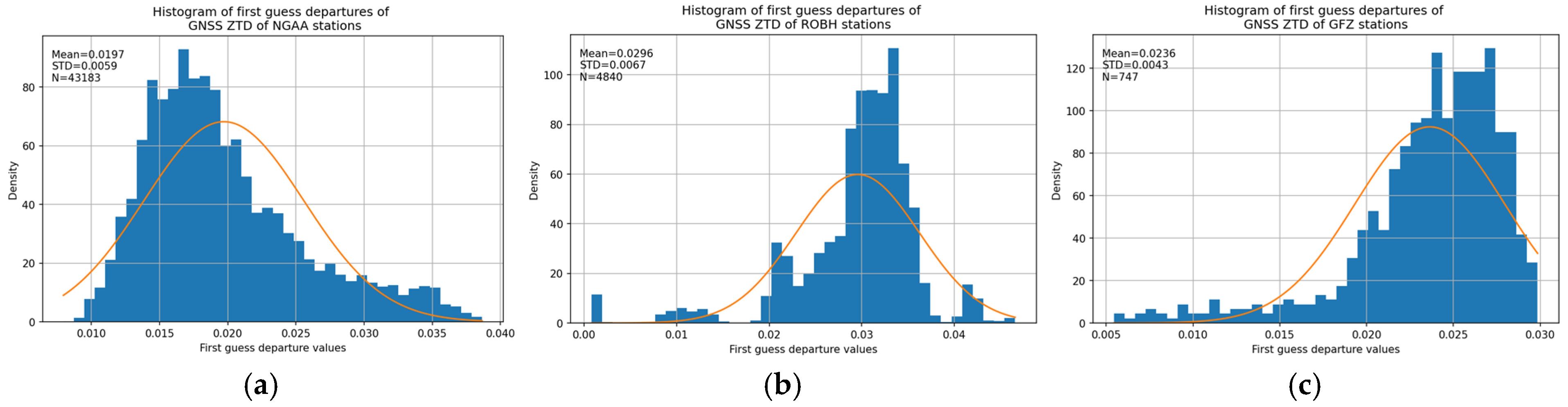
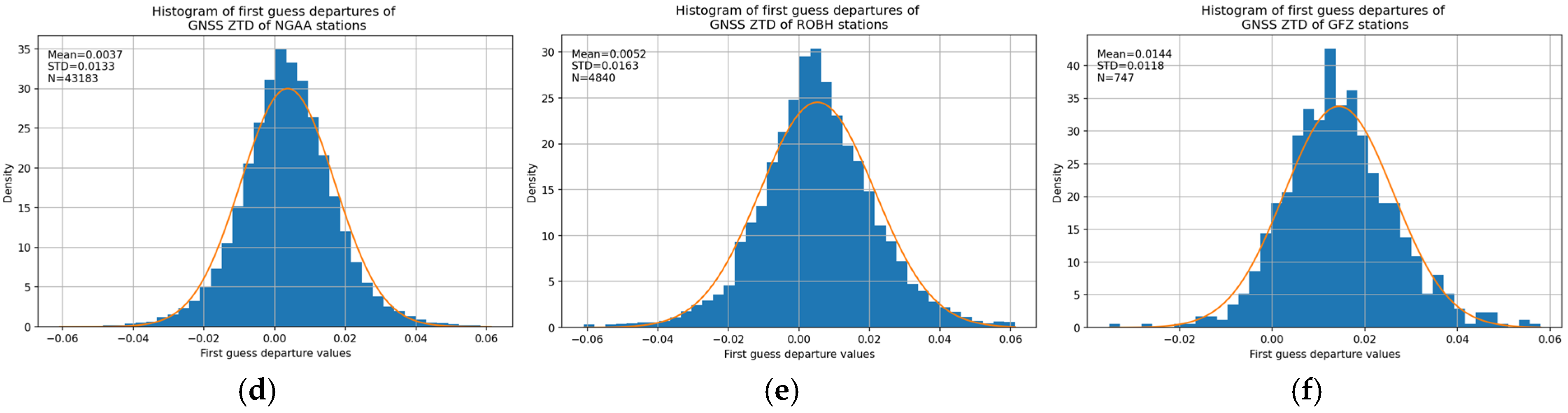
Here, we present histograms of the first-guess departures after bias correction of GNSS ZTD data from NGAA, Royal Observatory of Belgium hourly solution (ROBH), and GFZ stations, respectively, in Figure 3a–f, during a shorter period from the 7th to the end of June, which can give us an idea about the quality of ZTD data. These plots are valuable diagnostics because they illustrate how the observed ZTD values differ from their model-equivalent counterparts generated by the HARMONIE-AROME NWP system. The shape, mean, and spread of each distribution provide insight into the bias and variability of the GNSS data relative to the model, thereby serving as indicators of data quality and consistency across different networks. Filtering the ZTD departures into specific weather regimes (e.g., clear or rainy) leads to very small sample sizes and does not yield statistically meaningful histograms. We therefore use the full dataset, which provides stable and representative statistics for assessing ZTD data quality.

Figure 3a–c show the histograms of first-guess departures of GNSS ZTD observations from the NGAA, ROBH, and GFZ networks before bias correction. Each subplot displays the frequency distribution of departure values (blue bars) together with a fitted normal curve (orange line), allowing a direct visual assessment of the departure characteristics for each network. As seen from these figures, the biases are generally positive at all stations but differ in size. All three histograms are approximately Gaussian, consistent with the 3D-VAR assumption of random observation errors, but each exhibits a small positive mean, indicating the presence of systematic biases. The NGAA dataset (Figure 3a) displays the narrowest spread (mean = 19.7 mm, STD = 5.9 mm), reflecting high internal consistency and minimal bias. In contrast, the ROBH network (Figure 3b) shows a broader distribution (mean = 29.6 mm, STD = 6.7 mm), suggesting greater variability among stations and local atmospheric conditions. The GFZ observations (Figure 3c), although fewer in number (N = 747), exhibit a compact distribution (mean = 23.6 mm, STD = 4.3 mm) but a clear positive offset. Together, these panels illustrate the initial bias patterns across networks and highlight the need for bias-correction and thinning procedures to ensure that the assimilated ZTD observations satisfy the statistical assumptions of the 3D-VAR system.

Figure 3d–f present the corresponding histograms after bias-correction for NGAA, ROBH, and GFZ, respectively. These subplots follow the same format as the upper row, enabling a straightforward comparison between pre- and post-correction departure behaviour. The distributions remain approximately Gaussian but are now centred much closer to zero, demonstrating the effectiveness of the bias-correction procedure and the improved agreement between the GNSS ZTDs and the model first-guess fields. The NGAA network shows the smallest remaining bias (mean = 3.7 mm) and the narrowest spread (STD = 13.3 mm), confirming its overall data quality. The ROBH network (Figure 3e) retains a slightly broader distribution (mean = 5.2 mm, STD = 16.3 mm), consistent with its more heterogeneous station characteristics. The GFZ dataset (Figure 3f) still exhibits a small positive bias (mean = 14.4 mm) but maintains a relatively tight spread (STD = 11.8 mm), indicating a systematic offset rather than increased random noise. It is also important to note that GFZ stations are concentrated mainly in the southern part of the domain, whereas NGAA stations are more uniformly distributed, contributing to the robustness of the NGAA statistics. In short, the lower panels confirm that the bias-correction procedure successfully reduces systematic offsets and improves the consistency of ZTD observations across networks.

4.2.2. Differences in 2-m Temperature, Specific Humidity and 10-m Wind Components

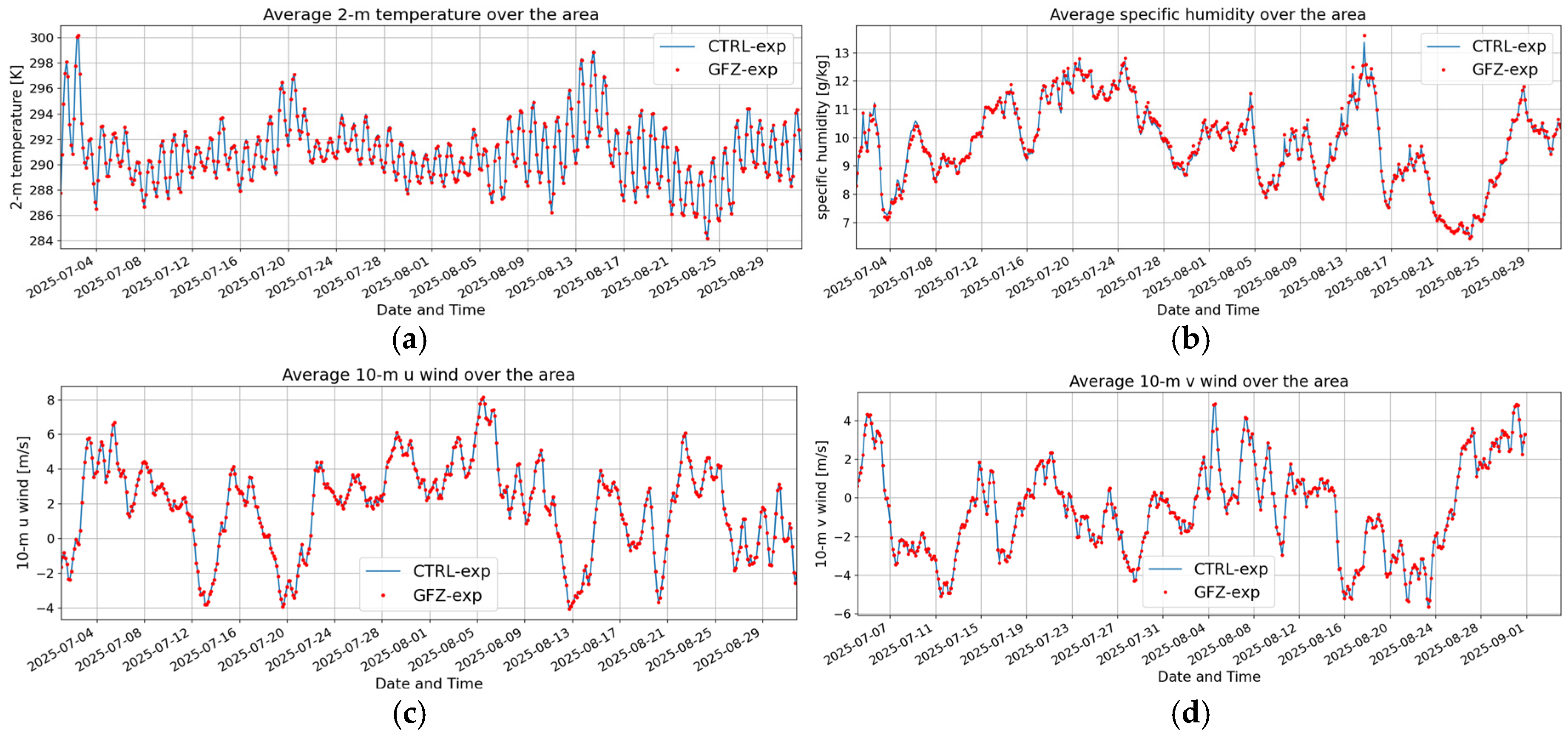
As shown in Figure 1, the north of Germany, which is in the southern part of the MetCoOp domain, was selected for the comparison, corresponding to the region where GFZ ZTD observations are available. This area is bounded by latitudes 52–56° N and longitudes 5–15° E. The parameters chosen to compare the two experiments are 2-m temperature, specific humidity, and 10-m wind zonal and meridional (u and v) components. Their average values over the area for 3-h forecasts are plotted and compared during June and August 2025.

Figure 4a shows the averaged 2-m temperature for CTRL-exp and GFZ-exp. Both experiments exhibit a consistent high-frequency oscillation associated with the diurnal cycle, with temperatures peaking during the daytime and decreasing at night. Over the two-month period, temperatures range from approximately 284 K (~11 °C) to 300 K (~27 °C). The inclusion of GFZ ZTDs does not substantially alter the overall temperature evolution. However, small differences are apparent at the extreme maxima and minima, indicating a subtle moderating effect on temperature extremes when GFZ data are assimilated. Temporally, the period begins with a pronounced warm episode in early July, followed by another peak in mid-August, and ends with a clear cooling trend towards late August, with the lowest temperatures occurring around 25 August.

Figure 4b presents the averaged 2-m specific humidity, expressed in grams of water vapour per kilogram of air (g kg⁻¹). The time series exhibits pronounced variability, with values ranging from about 6.5 g kg⁻¹ in late August to peaks exceeding 13.5 g kg⁻¹ around mid-August. Compared with temperature, specific humidity displays more complex, multi-day fluctuations, reflecting changes in synoptic-scale weather patterns and air-mass characteristics. While the overall evolution is very similar in both experiments, the simulation including GFZ data consistently shows slightly higher humidity values during moist periods. This difference is most evident during the major humidity peaks in late July and mid-August, suggesting that assimilation of GFZ ZTDs enhances the representation of atmospheric moisture under humid conditions. During drier periods, particularly between the 23rd and 25th of August, the two simulations converge closely, indicating strong agreement.

Figure 4c illustrates the averaged 10-m zonal (u-component) wind in m s⁻¹, where positive values indicate eastward flow and negative values indicate westward flow. The wind field is highly variable, with speeds generally fluctuating between −2 and +2 m s⁻¹. A notable exception occurs in mid-August, when eastward winds briefly intensify, reaching approximately 4.5 m s⁻¹. For most of the study period, the zonal wind evolution in both experiments is nearly identical, indicating that the assimilation of GFZ data has a negligible impact on the overall wind pattern. However, during the high-intensity wind event between 13 and 17 August, GFZ-exp exhibits slightly stronger peak values, suggesting a modest amplification of wind intensity under more dynamic atmospheric conditions.

Figure 4d shows the averaged 10-m meridional (v-component) wind, where positive values correspond to northward (southerly) flow and negative values vice versa. The v-wind demonstrates substantial variability, ranging from approximately −5.5 to +5 m s⁻¹. Several extended periods of southerly flow are evident, particularly in early July and early August, while sharp transitions to northerly flow occur in mid-July and late August. The two experiments again show very strong agreement, closely following the same synoptic-scale variations. Minor differences appear sporadically at extreme values—for example, around 24 August—where GFZ-exp indicates slightly stronger southward winds than CTRL-exp. When combined with the u-wind component, the v-wind allows reconstruction of the full near-surface wind vector; for instance, the event on 6 August is characterised by concurrent positive u- and v-wind components, indicating a strong south-westerly flow.

The primary differences between CTRL-exp and GFZ-exp arise in the magnitude of extreme values rather than in their timing and mostly in specific humidity, where GFZ-exp consistently produces higher peak moisture values. Similarly, wind components occasionally show slightly enhanced extremes during high-velocity events. In contrast, the 2-m temperature exhibits a mild damping of peak daytime values for GFZ-exp when GFZ data are included. These results indicate that assimilation of GFZ GNSS ZTD observations primarily refines the intensity of moisture and wind extremes—likely through improved representation of atmospheric moisture and surface–atmosphere interactions—while leaving the overall meteorological evolution largely unchanged.

4.2.3. Root Mean Square Error of Differences

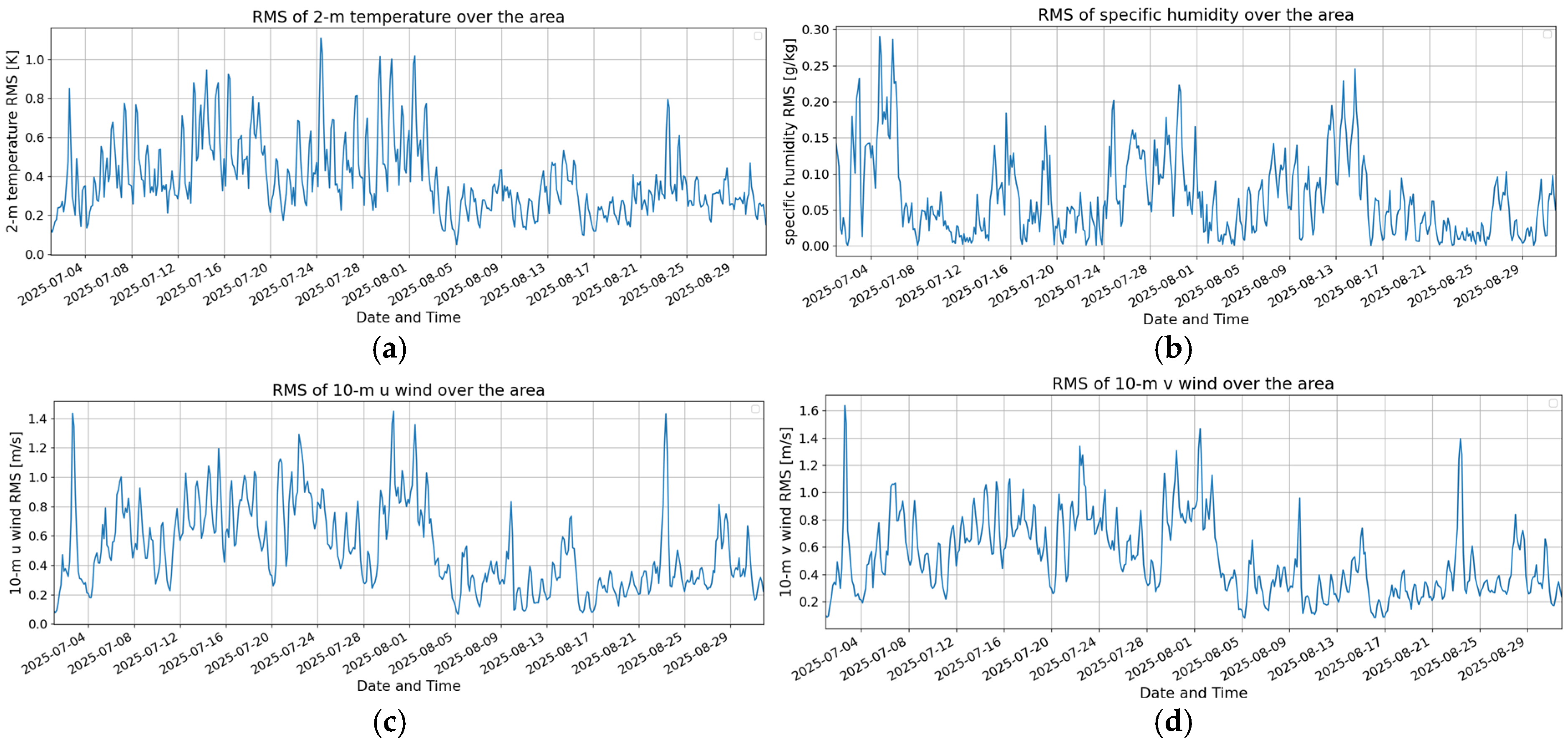
In order to highlight the differences, time series of the root mean square error (RMS) of differences between CTRL-exp and GFZ-exp for the same parameters discussed in the previous section are presented here.

Figure 5a shows the time series of the RMS differences in 2-m temperature, indicating a high level of agreement between CTRL-exp and GFZ-exp throughout the period. It exhibits intermittent increases during periods of enhanced atmospheric variability, occasionally reaching slightly above 1.25 K in a few cycles. The RMS differences in specific humidity, in Figure 5b, show the strongest sensitivity to the assimilation of GFZ ZTD in GFZ-exp. Occasional large deviations are observed during rapid moisture increases, particularly in early July, with GFZ-exp consistently producing slightly higher moisture content than CTRL-exp. In contrast, the differences largely disappear during drier conditions, suggesting that GFZ data primarily influence moisture estimates during dynamically active or humid periods, as expected. A similar pattern is observed for the wind components. The RMS differences for the 10-m u-wind, in Figure 5c, and v-wind, in Figure 5d, exhibit sharp increases during high-wind events, reaching approximately 1.4 m s⁻¹ and nearly 2.0 m s⁻¹, respectively. These peaks coincide with periods of strongest wind intensity, indicating that the assimilation of GFZ ZTD data leads to a modest amplification of wind extremes.

4.2.4. Average Profiles of Atmosphere

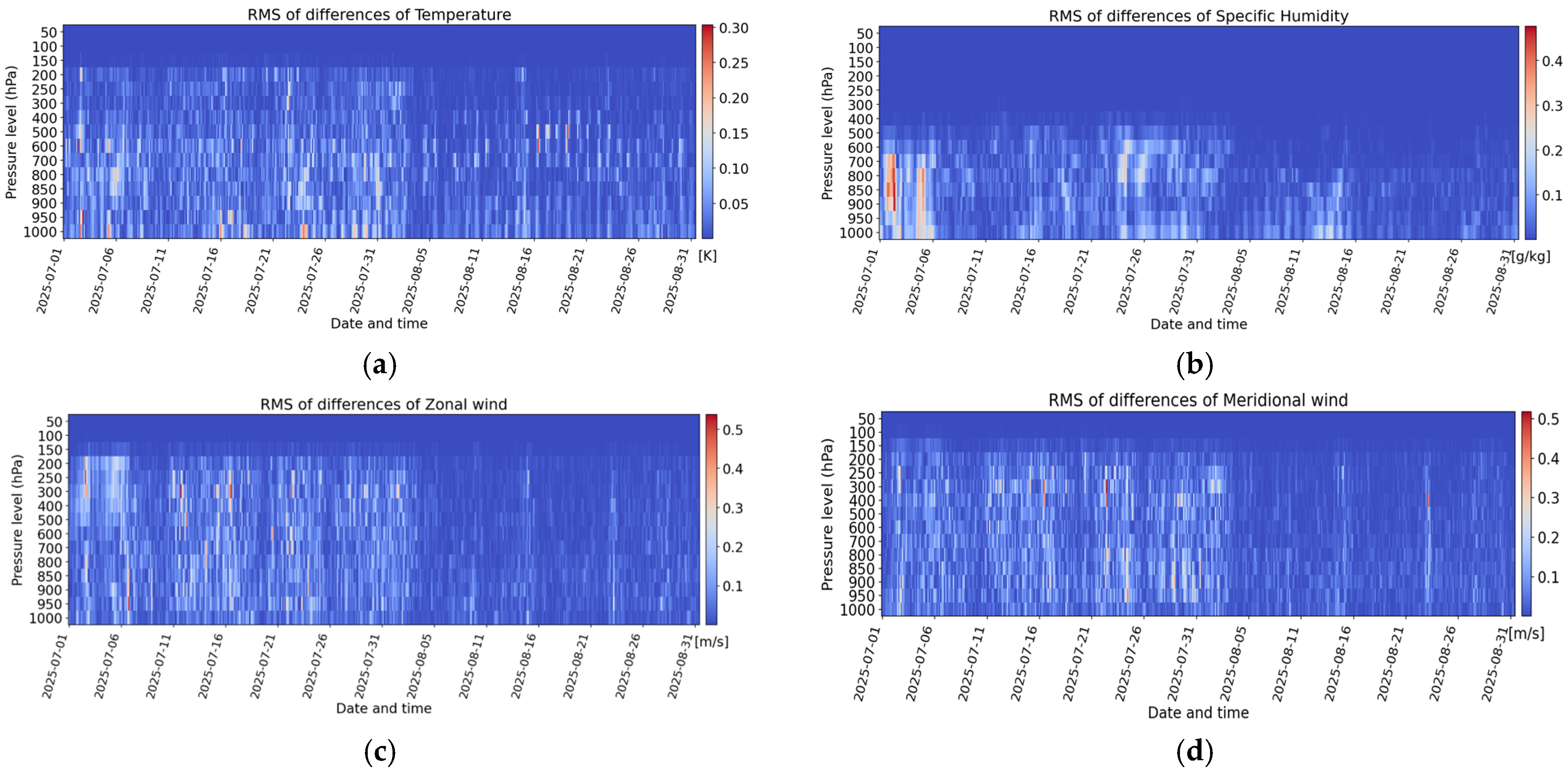
Here, we compare the same parameters’ averages but at different atmospheric levels ranging from 1000 to 50 hPa. The RMS differences between the two experiments are presented for these variables in the following matrices. The horizontal axis represents date and time at 3-hourly forecast cycles, while the vertical axis shows atmospheric pressure levels from the Earth’s surface (1000 hPa) up to the upper atmosphere (50 hPa).

Figure 6a shows the temperature RMS differences of the experiments, with the largest value reaching approximately 0.3 K near the surface in early July. As seen in Figure 6b, the RMS for specific humidity is concentrated below 850 hPa, highlighting the assimilation’s impact where moisture content is highest. Enhanced RMS values coincide with periods of strong humidity variability, confirming that ZTD assimilation primarily affects the moist boundary layer. The wind field’s response is captured in Figure 6c and Figure 5d, which respectively display the RMS differences for the zonal (u-wind) and meridional (v-wind) components. Figure 6c reveals a sharp 1.0 m s⁻¹ spike in u-wind near the jet-stream level, while Figure 6d shows a localised 0.6 m s⁻¹ adjustment in v-wind near the tropopause. These features suggest that the assimilation slightly modifies wind intensity at dynamically active levels. The results indicate that ZTD assimilation provides meaningful refinements to tropospheric variables but has negligible effects above 150 hPa, as evidenced by the consistent dark-blue regions across all four panels. This confirms that the assimilation’s influence is confined to the lower and middle troposphere, where GNSS-derived humidity information is most relevant.

4.2.5. Comparison with Radiosonde Data

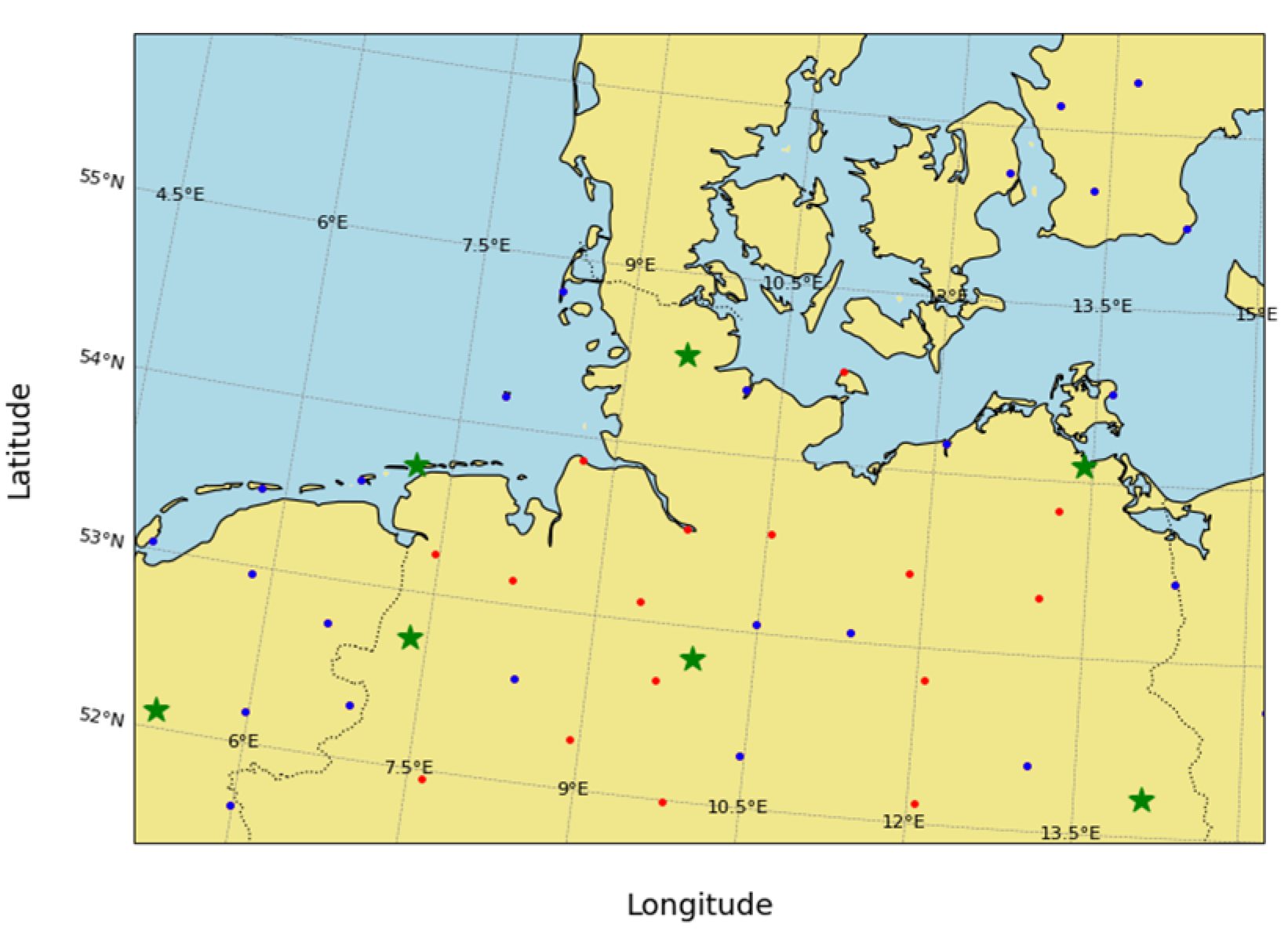
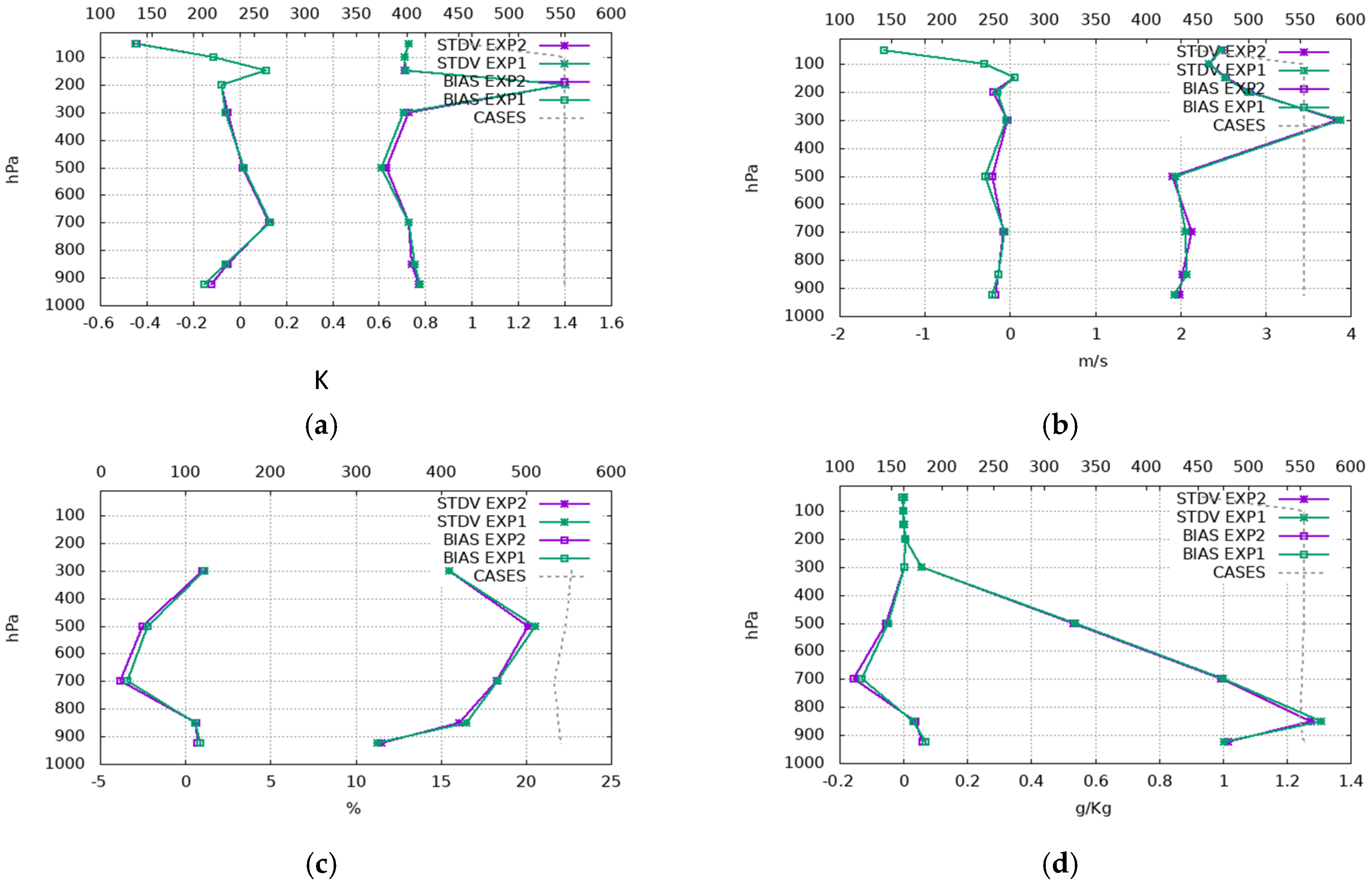
Thus far, the inclusion of GFZ ZTDs in the data assimilation process has been shown to induce measurable changes in temperature, humidity, and wind fields. To validate these results, radiosonde profiles are compared with the corresponding model fields from both experiments, CTRL-exp and GFZ-exp. For this purpose, we employed System Monitor, the official verification and evaluation platform for HARMONIE-AROME experiments. Radiosonde stations located within the southern part of the MetCoOp domain were selected for the analysis. The locations of these radiosonde stations are plotted on the map presented in Figure 7. As seen, three of these stations are rather far from the area covered by the GFZ stations.

The following plots present the differences between the observed radiosonde profiles and the model-simulated profiles from each experiment.

The vertical profile analysis over the southern part of the MetCoOp domain, during the period from July the 16th to 31st of August, indicates that the assimilation of GFZ ZTDs, GFZ-exp, leads to subtle yet targeted refinements in the atmospheric moisture structure, rather than a fundamental alteration of the vertical profile. The STDV of specific humidity, in Figure 8d, is nearly identical for both experiments, peaking at approximately 1.3 g/kg near the 850 hPa level. This peak corresponds to the upper portion of the Atmospheric Boundary Layer, where moisture variability is naturally high due to strong surface–atmosphere interactions. With increasing altitude and decreasing moisture content, the STDV steadily tapers toward zero above 300 hPa in the upper troposphere. Both experiments maintain a near-zero bias throughout most of the vertical column; however, a slight divergence emerges in the mid-to-lower troposphere. At the 700 hPa level, GFZ-exp exhibits a marginally stronger negative (dry) bias of approximately −0.15 g/kg compared to CTRL-exp. This adjustment is noteworthy, as the 700 hPa layer is commonly used to diagnose vertical motion and moisture transport processes. The assimilation of high-resolution GNSS ZTD data, which constrains the total vertically integrated water vapour, appears to recalibrate moisture content within these dynamically important layers. The vertical profiles confirm that the influence of GFZ data is most pronounced between the 925 hPa and 500 hPa levels. This suggests that while the large-scale and synoptic moisture structure remains stable, the GNSS-derived information provides a refined correction to the lower troposphere, potentially improving the representation of localised processes such as moisture transport, cloud formation, and latent heat exchange.

4.2.6. Maps of Differences over the Test Area

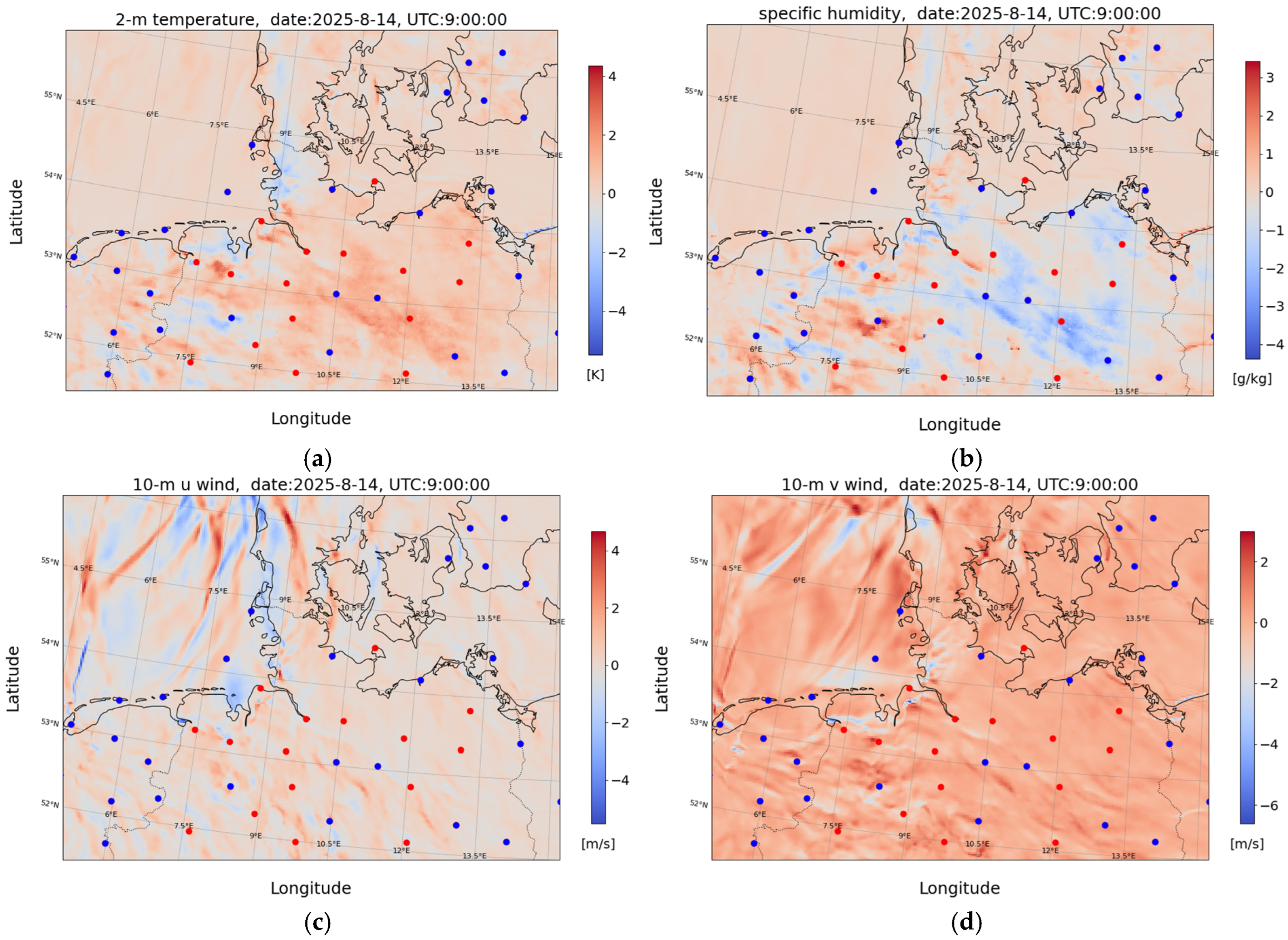
Since most of our results were about the average values of parameters and/or their differences, in this section, the maps of the differences are presented for a one-cycle forecast on 14 August 2025 at 9 UTC, based on Figure 5, in Figure 9, where the GFZ stations are shown by small red circles amongst the others in blue.

Figure 9a shows the spatial differences in 2-m temperature between CTRL-exp and GFZ-exp. Positive anomalies, primarily over land in northern Germany, indicate higher modelled temperatures in GFZ-exp, with local differences exceeding 4 K. Negative anomalies mark regions of relative cooling. These temperature differences are spatially clustered around GFZ GNSS stations, suggesting that the additional water vapour information modifies the local energy balance and enhances land–atmosphere interactions during mid-morning summer conditions. Both positive and negative increments naturally arise in an unbiased data assimilation system, reflecting the random-error corrections when the analysis departs from the background. In contrast, coastal and marine areas show minimal differences, indicating limited impact over the sea, as expected.

The corresponding specific humidity difference map in Figure 9b reveals a similarly structured but more heterogeneous response. Pronounced positive anomalies over land indicate higher moisture content in GFZ-exp, with local increases exceeding 3 g kg⁻¹, whilst negative anomalies below −4 g kg⁻¹ occur in some coastal and inland regions. Areas with higher humidity tend to align with positive temperature increments. This pattern reflects the radiative influence of moist air: increased water-vapour content absorbs more incoming solar energy before it reaches the surface, which reduces surface heating. The co-occurrence of these signals indicates a coupled thermodynamic adjustment within the boundary layer. This spatial variability helps explain the elevated RMS values observed in the humidity time series during rapidly evolving moisture events, highlighting the sensitivity of humidity fields to GNSS ZTD assimilation during dynamically active periods.

Differences in the 10-m u-wind, in Figure 9c, display a distinct spatial structure characterised by narrow bands of alternating positive and negative anomalies, particularly over the North Sea and the Danish peninsula. These streak-like features, with magnitudes reaching approximately ±4 m s⁻¹, indicate that the GFZ data primarily affect small-scale wind structures such as shear zones and convergence lines rather than the large-scale flow. Over northern Germany, the differences are weaker but still evident, often originating near GFZ observation sites. Although ZTD does not directly constrain wind, the humidity- and temperature-related adjustments introduced by the additional observations can modify mass-wind balances, which explains the fine-scale wind responses. This behaviour is consistent with the intermittent peaks seen in the u-wind error statistics during periods of strong winds.

A comparable response is evident in Figure 9d for the 10-m v-wind. Dominance of positive anomalies over both land and adjacent maritime areas indicates enhanced northward (southerly) flow in GFZ-exp. As with the u-wind, linear streaks of alternating sign are apparent, particularly over marine regions, with differences ranging from approximately −6 to +3 m s⁻¹. These spatial patterns correspond to periods of elevated wind error and suggest that the assimilation of GFZ ZTDs induces localised adjustments to the near-surface pressure gradients that govern wind intensity.

5. Discussion

The assimilation of GNSS ZTDs primarily modifies the integrated water vapour field, and these increments propagate through the boundary layer via coupled thermodynamic and dynamical processes. Increased integrated water vapour enhances near-surface humidity, which alters the surface-energy balance by increasing short-wave absorption and latent-heat fluxes while reducing sensible-heat transfer. This produces small but coherent temperature adjustments that depend on local land–sea contrast and surface characteristics. Moisture increments also modify boundary-layer stability and turbulence, influencing the vertical mixing of momentum. Through the mass–wind balance constraint in variational assimilation, humidity- and temperature-related increments induce localised adjustments in near-surface winds, particularly in regions with strong gradients or complex terrain. The coexistence of positive and negative anomalies in temperature, humidity, and wind therefore reflects the combined effects of integrated water vapour increments, boundary-layer mixing, surface heterogeneity, and the unbiased nature of the variational assimilation system. These mechanisms explain the spatially structured responses observed in Figure 5, Figure 6 and Figure 9.

The results of this study are consistent with, and extend, the existing literature on the assimilation of GNSS ZTD data in high-resolution NWP models. Our findings demonstrate that the inclusion of GFZ ZTD observations produces localised, still meaningful refinements in atmospheric moisture and temperature fields, broadly reinforcing trends reported in previous studies.

Our results can be positioned within the broader European experience with GNSS ZTD assimilation. European regional systems consistently report that ZTDs exert their strongest influence in the mid-to-lower troposphere, and our analysis confirms this behaviour by identifying coherent humidity and temperature refinements in the 925–500 hPa layer. The spatial organisation of these increments—localised moistening around stations and elongated correction zones aligned with moisture-transport pathways—mirrors patterns documented in European studies and highlights the importance of network density in determining impact. In our case, the enhanced GFZ coverage in the southern MetCoOp domain provides a denser upstream constraint than in earlier Fennoscandian experiments, allowing us to demonstrate how GNSS observations over northern Germany can meaningfully improve humidity analyses further downstream in Fennoscandia.

Although 3D-VAR cannot retrieve wind information directly from ZTD, the fine-scale wind adjustments we observe are dynamically consistent with the mass–wind balance effects simulated in regional models. These adjustments arise from humidity- and temperature-related increments propagating through pressure-gradient and turbulent processes. The stronger impacts during high-variability summer periods reinforce the established European evidence that hourly GNSS ZTD observations provide valuable moisture constraints for short-range forecasting and nowcasting.

Beyond these comparisons, our results align with broader European GNSS ZTD assimilation studies [11,13,53], which consistently report improvements in lower-tropospheric humidity and boundary-layer structure. In our case, the largest refinements occur in the 925–700 hPa layer and over northern Germany, where GNSS station density is highest, with typical reductions of 0.1–0.3 g kg⁻¹ in specific humidity and 0.1–0.3 K in temperature. These magnitudes are comparable to those reported in previous European studies, confirming the regional applicability of ZTD assimilation in moisture-sensitive environments.

6. Concluding Remarks

This study evaluated the impact of assimilating additional Global Navigation Satellite Systems (GNSS)-derived zenith total delays (ZTDs) from the Geoscience Research Centre (GFZ) network in northern Germany on short-range forecasts within the convection-permitting Meteorological Cooperation on Operational Numerical Weather Prediction (MetCoOp) and High-Resolution Limited Area Model—Applications of Research to Operations at Mesoscale (HARMONIE–AROME) system. Because moisture and temperature advection into Fennoscandia frequently originates from the west and southwest, strengthening ZTD coverage in the southern part of the MetCoOp domain is of particular relevance for improving humidity analyses. By conducting two parallel experiments—one using the operational ZTD dataset and one augmented with GFZ observations—we quantified the influence of enhanced ZTD density on the analysis and forecast fields.

The results demonstrate that assimilating GFZ ZTDs leads to a more refined representation of mid-to-lower-tropospheric moisture (500–925 hPa), with clearer horizontal gradients and improved boundary-layer structure. Although domain-averaged differences in specific humidity (~1.3 g kg⁻¹) and temperature (~1 K) remain modest, spatial patterns reveal systematic improvements over land, particularly in regions where the operational ZTD network is sparse. These findings highlight the sensitivity of high-resolution NWP systems to additional GNSS humidity information and confirm that ZTD observations provide valuable constraints on latent-heat-related processes. Expanding GNSS ZTD coverage in the southern MetCoOp domain enhances the quality of humidity analyses and contributes to more accurate short-range forecasts. The results support continued integration of additional GNSS networks into operational NWP and motivate further research on optimising ZTD thinning, bias-correction, and the combined assimilation of ZTD and slant delays in convection-permitting systems.

In addition to these general findings, the improvements observed in this study are consistent with previous GNSS ZTD assimilation efforts, which similarly report enhanced moisture analyses and boundary-layer structure. The largest refinements in our experiment occur in the 925–700 hPa layer and over northern Germany, where GNSS station density is highest. Typical reductions in specific-humidity and temperature biases are on the order of 0.1–0.3 g kg⁻¹ and 0.1–0.3 K, respectively, demonstrating the regional applicability of ZTD assimilation in moisture-sensitive environments. The experiment also evaluates only the operational MetCoOp/HARMONIE–AROME configuration and focuses solely on ZTD assimilation, meaning that potential benefits from slant total delays or multi-GNSS combinations were not assessed. These aspects suggest several directions for future work, including examining additional weather regimes within MetCoOp, exploring the role of slant total delays in convection-permitting systems, and assessing how GNSS humidity information interacts with other observation types such as radar or satellite data.

References

1. Seity, Y.; Brousseau, P.; Malardel, S.; Hello, G.; Benard, P.; Bouttier, F.; Lac, C.; Masson, V. The AROME-France convective-scale operational model. Mon. Weather Rev. 2011, 139, 976–991. [Google Scholar] [CrossRef] [Scilit]
2. Bengtsson, L.; Andræ, U.; Aspelien, T.; Batrak, Y.; Calvo, J.; de Rooy, W.; Gleeson, E.; Hansen-Sass, B.; Homleid, M.; Hortal, M.; et al. The HARMONIE–AROME model configuration in the ALADIN–HIRLAM NWP system. Mon. Weather Rev. 2017, 145, 1919–1935. [Google Scholar] [CrossRef] [Scilit]
3. Eresmaa, R.; Andrae, U.; Berggren, L.; Bremnes, J.B.; Fortelius, C.; Frogner, I.-L.; Gregow, E.; Grote, R.; Ridal, M.; Vignes, O.; et al. The operational forecast process at MetCoOp. Bull. Am. Meteorol. Soc. 2026, 107, E946–E963. [Google Scholar] [CrossRef] [Scilit]
4. Vedel, H.; Huang, X.-Y. Impact of ground-based GPS data on numerical weather prediction. J. Meteorol. Soc. Jpn. 2004, 82, 459–472. [Google Scholar] [CrossRef] [Scilit]
5. Le Dimet, F.-X.; Talagrand, O. Variational algorithms for analysis and assimilation of meteorological observations: Theoretical aspects. Tellus A 1986, 38, 97–110. [Google Scholar] [CrossRef] [Scilit]
6. Gustafsson, N.; Huang, X.-Y.; Yang, X.; Mogensen, K.; Lindskog, M.; Vignes, O.; Wilhelmsson, T.; Thorsteinsson, S. Four-dimensional variational data assimilation for a limited-area model. Tellus A 2012, 64, 14985. [Google Scholar] [CrossRef] [Scilit]
7. Poli, P.; Moll, P.; Rabier, F.; Desroziers, G.; Chapnik, B.; Berre, L.; Healy, S.B.; Andersson, E.; Guelai, F.Z.E. Forecast impact studies of ZTD data from European NRT GPS stations in Météo-France 4D-Var. J. Geophys. Res. Atmos. 2007, 112, D06114. [Google Scholar] [CrossRef] [Scilit]
8. Macpherson, S.R.; Deblonde, G.; Aparicio, J.M.; Casati, B. Impact of NOAA ground-based GPS observations on the Canadian regional analysis and forecast system. Mon. Weather Rev. 2008, 136, 2727–2746. [Google Scholar] [CrossRef] [Scilit]
9. Boniface, K.; Ducrocq, V.; Jaubert, G.; Yan, X.; Brousseau, P.; Masson, F.; Champollion, C.; Chéry, J.; Doerflinger, E. Impact of high-resolution data assimilation of GPS zenith delay on Mediterranean heavy rainfall forecasting. Ann. Geophys. 2009, 27, 2739–2753. [Google Scholar] [CrossRef] [Scilit]
10. Yan, X.; Ducrocq, V.; Jaubert, G.; Brousseau, P.; Poli, P.; Champollion, C.; Flamant, C.; Boniface, K. The benefit of GPS zenith delay assimilation on high-resolution quantitative precipitation forecast of the COPS cases IOP 9. Q. J. R. Meteorol. Soc. 2009, 135, 1788–1800. [Google Scholar] [CrossRef] [Scilit]
11. Lindskog, M.; Ridal, M.; Thorsteinsson, S.; Ning, T. Data assimilation of GNSS ZTD from a Nordic processing centre. Atmos. Chem. Phys. 2017, 17, 13983–13998. [Google Scholar] [CrossRef] [Scilit]
12. Skamarock, W.C.; Klemp, J.B.; Dudhia, J.; Gill, D.O.; Liu, Z.; Berner, J.; Wang, W.; Powers, J.G.; Duda, M.G.; Barker, D.M.; et al. A Description of the Advanced Research WRF Version 4; NCAR Technical Note NCAR/TN-556+STR; National Center for Atmospheric Research: Boulder, CO, USA, 2019. [Google Scholar] [CrossRef]
13. Rohm, W.; Guzikowski, J.; Wilgan, K.; Kryza, M. 4D-Var assimilation of GNSS ZTD and PWV into WRF. Atmos. Meas. Tech. 2019, 12, 345–361. [Google Scholar] [CrossRef] [Scilit]
14. Lagasio, M.; Parodi, A.; Pulvirenti, L.; Meroni, A.N.; Boni, G.; Pierdicca, N.; Marzano, F.S.; Luini, L.; Venuti, G.; Realini, E.; et al. A synergistic use of a high-resolution NWP model and EO products to improve precipitation forecast. Remote Sens. 2019, 11, 2387. [Google Scholar] [CrossRef] [Scilit]
15. Giannaros, C.; Kotroni, V.; Lagouvardos, K.; Giannaros, T.M.; Pikridas, C. Assessing the impact of GNSS ZTD data assimilation into the WRF modeling system during high-impact rainfall events over Greece. Remote Sens. 2020, 12, 383. [Google Scholar] [CrossRef] [Scilit]
16. Caldas-Alvarez, A.; Khodayar, S. Assessing atmospheric moisture effects on heavy precipitation during HyMeX IOP16 using GPS nudging and dynamical downscaling. Nat. Hazards Earth Syst. Sci. 2020, 20, 2753–2776. [Google Scholar] [CrossRef] [Scilit]
17. Kalnay, E.; Mote, S.; Da, C. Earth System Modeling, Data Assimilation and Predictability: Atmosphere, Oceans, Land and Human Systems, 2nd ed.; Cambridge University Press: Cambridge, UK, 2024. [Google Scholar]
18. Mascitelli, A.; Federico, S.; Fortunato, M.; Avolio, E.; Torcasio, R.C.; Realini, E.; Mazzoni, A.; Transerici, C.; Crespi, M.; Dietrich, S. Data assimilation of GPS-ZTD into the RAMS model through 3D-Var. Meas. Sci. Technol. 2019, 30, 055801. [Google Scholar] [CrossRef] [Scilit]
19. Mascitelli, A.; Federico, S.; Torcasio, R.; Dietrich, S. Assimilation of GPS ZTD estimates in the RAMS NWP model: Impact studies over central Italy. Adv. Space Res. 2021, 68, 4783–4793. [Google Scholar] [CrossRef] [Scilit]
20. Li, J.; Lu, C.; Zheng, Y.; He, B.; Wang, Q.; Dick, G. Synergistic assimilation of radar-derived precipitation and GNSS ZTD to improve heavy rainfall forecasts. IEEE Trans. Geosci. Remote Sens. 2025, 63, 4103917. [Google Scholar] [CrossRef] [Scilit]
21. Torcasio, R.C.; Mascitelli, A.; Realini, E.; Barindelli, S.; Tagliaferro, G.; Puca, S.; Dietrich, S.; Federico, S. The impact of global navigation satellite system (GNSS) zenith total delay data assimilation on the short-term precipitable water vapor and precipitation forecast over Italy using the Weather Research and Forecasting (WRF) model. Nat. Hazards Earth Syst. Sci. 2023, 23, 3319–3336. [Google Scholar] [CrossRef] [Scilit]
22. Wagner, A.; Fersch, B.; Yuan, P.; Rummler, T.; Kunstmann, H. Assimilation of GNSS and synoptic data in a convection-permitting limited-area model: Improvement of simulated tropospheric water vapor content. Front. Earth Sci. 2022, 10, 869504. [Google Scholar] [CrossRef] [Scilit]
23. Zheng, Y.; Lu, C.; Wu, Z.; Guan, Z.; Li, J.; Wang, Z.; Liu, C. Assimilation of high-resolution GNSS tropospheric delays and its effects on a severe convective event nowcasting. Atmos. Res. 2025, 314, 107785. [Google Scholar] [CrossRef] [Scilit]
24. Zhang, Z.; Liu, M.; Zhang, W.; Lou, Y.; Soja, B. Assimilating ground-based and high-dynamic airborne GNSS zenith total delays into numerical weather predictions. IEEE Trans. Geosci. Remote Sens. 2025, 63, 1–9. [Google Scholar] [CrossRef] [Scilit]
25. Thundathil, R.; Zus, F.; Dick, G.; Wickert, J. Assimilation of global navigation satellite system (GNSS) zenith delays and tropospheric gradients: A sensitivity study utilizing sparse and dense station networks. Atmos. Meas. Tech. 2025, 18, 4907–4922. [Google Scholar] [CrossRef] [Scilit]
26. Hofmann-Wellenhof, B.; Lichtenegger, H.; Wasle, E. GNSS: Global Navigation Satellite Systems, GPS, GLONASS, Galileo, and More; Springer: Vienna, Austria, 2008. [Google Scholar]
27. Liu, J.; Sun, Z.; Liang, H.; Xu, X.; Wu, P. Precipitable water vapor on the Tibetan Plateau estimated by GPS, water vapor radiometer, radiosonde, and numerical weather prediction analysis and its impact on the radiation budget. J. Geophys. Res. Atmos. 2005, 110, D17106. [Google Scholar] [CrossRef] [Scilit]
28. Vázquez, B.G.E.; Grejner-Brzezinska, D.A. GPS-PWV estimation and validation with radiosonde data and numerical weather prediction model in Antarctica. GPS Solut. 2013, 17, 29–39. [Google Scholar] [CrossRef] [Scilit]
29. Liou, Y.; Teng, Y.; Van Hove, T.; Liljegren, J.C. Comparison of precipitable water observations in the near tropics by GPS, microwave radiometer, and radiosondes. J. Appl. Meteorol. Climatol. 2001, 40, 5–15. [Google Scholar] [CrossRef] [Scilit] [PubMed]
30. Niell, A.E. Global mapping functions for atmospheric delay at radio wavelengths. J. Geophys. Res. Solid Earth 1996, 100, 3227–3246. [Google Scholar] [CrossRef] [Scilit]
31. Böhm, J.; Werl, B.; Schuh, H. Troposphere mapping functions for GPS and VLBI from ECMWF operational analysis data. J. Geophys. Res. Solid Earth 2006, 111, B02406. [Google Scholar] [CrossRef] [Scilit]
32. Dach, R.; Lutz, S.; Walser, P.; Fridez, P. (Eds.) Bernese GNSS Software Version 5.2: User Manual; Bern Open Publishing: Bern, Switzerland, 2015. [Google Scholar] [CrossRef] [Scilit]
33. Gendt, G.; Dick, G.; Reigber, C.; Tomassini, M.; Liu, Y.; Ramatschi, M. Near real-time GPS water vapor monitoring for numerical weather prediction in Germany. J. Meteorol. Soc. Jpn. 2004, 82, 361–370. [Google Scholar] [CrossRef] [Scilit]
34. Zumberge, J.F.; Heflin, M.B.; Jefferson, D.C.; Watkins, M.M.; Webb, F.H. Precise point positioning for the efficient and robust analysis of GPS data from large networks. J. Geophys. Res. Solid Earth 1997, 102, 5005–5017. [Google Scholar] [CrossRef] [Scilit]
35. Herring, T.A.; King, R.W.; Floyd, M.A.; McClusky, S.C. GAMIT Reference Manual: GPS Analysis at MIT (Release 10.7); Massachusetts Institute of Technology: Cambridge, MA, USA, 2018. [Google Scholar]
36. Vedel, H.; Mogensen, K.S.; Huang, X.-Y. Calculation of zenith delays from meteorological data: Comparison of NWP model, radiosonde and GPS delays. Phys. Chem. Earth A 2001, 26, 497–502. [Google Scholar] [CrossRef] [Scilit]
37. Saastamoinen, J. Contributions to the theory of atmospheric refraction. Bull. Géod. 1972, 105, 279–298. [Google Scholar] [CrossRef] [Scilit]
38. Bevis, M.; Businger, S.; Herring, T.A.; Rocken, C.; Anthes, R.A.; Ware, R.H. GPS meteorology: Remote sensing of atmospheric water vapor using the Global Positioning System. J. Geophys. Res. Atmos. 1992, 97, 15787–15801. [Google Scholar] [CrossRef] [Scilit]
39. Dee, D.P. Bias and data assimilation. Q. J. R. Meteorol. Soc. 2005, 131, 3323–3343. [Google Scholar] [CrossRef] [Scilit]
40. Dee, D.P. Variational bias correction of radiance data in the ECMWF system. In Proceedings of the ECMWF Workshop on Assimilation of High Spectral Resolution Sounders in NWP, Reading, UK, 28 June–1 July 2004; pp. 97–112. [Google Scholar]
41. Sánchez-Arriola, J.; Lindskog, M.; Thorsteinsson, S.; Bojarova, J. Variational bias correction of GNSS ZTD in HARMONIE. J. Appl. Meteorol. Climatol. 2016, 55, 1259–1276. [Google Scholar] [CrossRef] [Scilit]
42. Desroziers, G.; Berre, L.; Chapnik, B.; Poli, P. Diagnosis of observation, background and analysis-error statistics in observation space. Q. J. R. Meteorol. Soc. 2005, 131, 3385–3396. [Google Scholar] [CrossRef] [Scilit]
43. Masson, V.; Le Moigne, P.; Martin, E.; Faroux, S.; Alias, A.; Alkama, R.; Belamari, S.; Barbu, A.; Boone, A.; Bouyssel, F.; et al. The SURFEXv7.2 land and ocean surface platform. Geosci. Model Dev. 2013, 6, 929–960. [Google Scholar] [CrossRef] [Scilit]
44. Berre, L. Estimation of synoptic and mesoscale forecast error covariances in a limited-area model. Mon. Weather Rev. 2000, 128, 644–667. [Google Scholar] [CrossRef] [Scilit]
45. Dach, R.; Hugentobler, U.; Fridez, P.; Meindl, M. Bernese GPS Software, version 5.2; Astronomical Institute, University of Bern: Bern, Switzerland, 2007.
46. Lyard, F.; Lefevre, F.; Letellier, T.; Francis, O. Modelling the global ocean tides: Modern insights from FES2004. Ocean Dyn. 2006, 56, 394–415. [Google Scholar] [CrossRef] [Scilit]
47. Schmid, R.; Steigenberger, P.; Gendt, G.; Ge, M.; Rothacher, M. Generation of a consistent absolute phase center correction model for GPS antennas. J. Geod. 2007, 81, 781–798. [Google Scholar] [CrossRef] [Scilit]
48. Bruyninx, C. The EUREF Permanent Network: A multidisciplinary network serving surveyors as well as scientists. GeoInformatics 2004, 7, 32–35. [Google Scholar]
49. Dow, J.M.; Neilan, R.E.; Rizos, C. The International GNSS Service in a changing landscape of Global Navigation Satellite Systems. J. Geod. 2009, 83, 191–198. [Google Scholar] [CrossRef] [Scilit]
50. McCarthy, D.D. IERS Conventions (1996); IERS Technical Note 21; International Earth Rotation Service: Paris, France, 1996. [Google Scholar]
51. Pagiatakis, S.D. Ocean Tide Loading, Body Tide and Polar Motion Effects on Very Long Baseline Interferometry; Technical Report No. 92; Department of Surveying Engineering, University of New Brunswick: Fredericton, NB, Canada, 1982. [Google Scholar]
52. Hersbach, H.; Bell, B.; Berrisford, P.; Hirahara, S.; Horányi, A.; Muñoz-Sabater, J.; Nicolas, J.; Peubey, C.; Radu, R.; Schepers, D.; et al. The ERA5 global reanalysis. Q. J. R. Meteorol. Soc. 2020, 146, 1999–2049. [Google Scholar] [CrossRef] [Scilit]
53. Bennitt, G.V.; Jupp, A. Operational assimilation of GPS zenith total delay observations into the Met Office numerical weather prediction models. Mon. Weather Rev. 2012, 140, 2706–2719. [Google Scholar] [CrossRef] [Scilit]
Figure 1. Allowlisted GNSS stations based on 50 km thinning distance for the MetCoOp domain.
Applsci 16 08699 g001
Figure 2. Time series of variational bias-correction coefficients for three newly assimilated GFZ stations from 15th of June to 7th of July 2025. The coefficients start from zero on 15 June and stabilise in early July. The stabilised values confirm that the bias-correction system reached equilibrium before the evaluation period. VARBC stands for variational bias-correction.
Applsci 16 08699 g002
Figure 3. Histograms of first-guess departures of GNSS ZTD stations from (a) NGAA, (b) ROBH, and (c) GFZ before bias correction, and (df) the corresponding distributions after bias correction. Blue bars show the frequency distribution of departure values, and orange curves indicate fitted normal distributions. Each subplot lists the mean, standard deviation, and sample size. Panels (ac) illustrate the initial positive biases and network-dependent spread, while panels (df) demonstrate how the bias-correction procedure recentres the distributions and reduces systematic offsets.
Applsci 16 08699 g003aApplsci 16 08699 g003b
Figure 4. Time-series averages of (a) 2-m temperature [K], (b) 2-m specific humidity [g/kg], (c) 10-m u-wind component [m/s], and (d) 10-m v-wind component [m/s] for CTRL-exp (without GFZ ZTD) and GFZ-exp (with GFZ ZTD) over the selected area. Orange and blue lines represent the two experiments, showing nearly identical temporal evolution with minor differences during synoptic events, indicating that the assimilation of GFZ ZTDs has limited impact on near-surface meteorological fields.
Applsci 16 08699 g004
Figure 5. Time series of the root mean square error (RMS) of the differences between CTRL-exp and GFZ-exp for (a) 2-m temperature (K), (b) 2-m specific humidity (g kg−1), (c) 10-m u-wind component (m s−1), and (d) 10-m v-wind component (m s−1). RMS values remain low throughout the period, indicating that assimilation of GFZ ZTDs introduces only minor changes to near-surface meteorological fields, with slightly reduced RMS during moist and windy episodes.
Applsci 16 08699 g005
Figure 6. Plots of RMS of differences between (a) temperature, (b) specific humidity, (c) zonal wind (u-wind) and (d) meridional wind (v-wind) of CTRL-exp and GFZ-exp. Blue shading indicates small RMS differences, while warmer colors mark larger discrepancies. The results show that assimilation of GFZ ZTDs produces only minor changes, with slightly higher RMS values near the lower troposphere during moist or windy episodes.
Applsci 16 08699 g006
Figure 7. Locations of GNSS stations used for computing ZTDs: blue circles those active in the MetCoOp system, and red circles those from GFZ, and radiosonde stations by green stars.
Applsci 16 08699 g007
Figure 8. Vertical profile differences of CTRL-exp (EXP 1)and GFZ-exp (EXP2) with radiosonde data (16 July 2025–31 August 2025): (a) temperature [K], (b) wind speed [m/s], (c) relative humidity [%], and (d) specific humidity [g/kg].
Applsci 16 08699 g008
Figure 9. Spatial distribution of differences between CTRL-exp and GFZ-exp for (a) 2-m temperature [K], (b) 2-m specific humidity [g kg−1], (c) 10-m u-wind [m s−1], and (d) 10-m v-wind component [m s−1].
Applsci 16 08699 g009
Disclaimer/Publisher’s Note: The statements, opinions and data contained in all publications are solely those of the individual author(s) and contributor(s) and not of MDPI and/or the editor(s). MDPI and/or the editor(s) disclaim responsibility for any injury to people or property resulting from any ideas, methods, instructions or products referred to in the content.