Article

Spatially Enhanced Modeling of Debris Flow Susceptibility Using Topographic and Micro-Geomorphic Indicators

1
The Institute of Geological Survey, China University of Geosciences (Wuhan), Wuhan 430074, China
2
Faculty of Engineering, China University of Geosciences (Wuhan), Wuhan 430074, China
*
Author to whom correspondence should be addressed.
Appl. Sci. 2026, 16(17), 8585; https://doi.org/10.3390/app16178585 (registering DOI)
Submission received: 8 June 2026 / Revised: 4 August 2026 / Accepted: 5 August 2026 / Published: 28 August 2026
(This article belongs to the Section Environmental Sciences)

Abstract

Mapping debris flow susceptibility is essential for disaster risk reduction in mountainous regions. This study proposes a spatially enhanced modeling framework to evaluate these mass-wasting hazards. The framework integrates conventional topographic parameters with localized micro-geomorphic indicators to assess susceptibility in Bomi County, Tibet. Extracted geomorphological variables include the Topographic Position Index (TPI), surface roughness, local relief, and flow accumulation. We applied multi-scale moving window operations to explicitly quantify spatial heterogeneity and sediment connectivity. This approach systematically evaluates the influence of localized landscape variations on debris flow kinematics. The Random Forest (RF) algorithm was utilized to construct the spatial susceptibility model, and the area under the receiver operating characteristic curve (AUC) quantified its predictive capability. The proposed framework achieves a high predictive accuracy with an AUC of 0.9434. Feature importance analysis demonstrates that micro-geomorphic variables contribute significantly to the predictions; specifically, TPI and local relief primarily drive the overall classification performance. Furthermore, the multi-scale spatial enrichment enables the model to effectively capture complex physical interactions across the terrain. Ultimately, this methodology provides an objective, spatially explicit tool for mass-wasting susceptibility mapping, offering reliable data to support disaster prevention and risk management in the Tibetan Plateau and similar highly incised alpine ecosystems.

1. Introduction

Debris flows—frequently initiated by rockfalls and collapses in steep terrain—are rapid, destructive mass movements consisting of water, sediment, and debris [1,2]. These geohazards pose significant threats to lives, infrastructure, and mountainous ecosystems [3]. Over the past several decades, global warming has systematically amplified the frequency and magnitude of these mass-wasting events. Specifically, the intensification of extreme hourly rainfall and accelerated glacial melting in high-altitude environments directly drive this increasing trend [4,5,6]. Furthermore, a complex interplay of regional tectonics, local topography, surface hydrology, and climatic factors strictly controls the initiation of these geological events. Consequently, precise susceptibility mapping is essential for effective disaster risk management and regional spatial planning [7,8].
Modern remote sensing technologies have transformed the capacity to characterize terrain properties at fine spatial scales [9]. The integration of high-resolution Digital Elevation Models (DEMs), acquired via satellite imagery, Light Detection and Ranging (LiDAR), and Unmanned Aerial Vehicles (UAVs), directly facilitates the precise spatial modeling of debris flow susceptibility [10,11].
To address accuracy challenges in data-driven assessments, recent studies demonstrate that optimized semi-supervised negative sampling strategies eliminate spatial bias and improve the predictive reliability of tree-based machine learning models [12]. Additionally, progressive mapping frameworks effectively delineate material source areas and enhance regional predictions by coupling watershed-based extraction units with hybrid algorithms [13]. Recent evaluations of grid-based models highlight the sensitivity of susceptibility mapping to spatial sampling schemes. These studies establish that explicitly distinguishing specific geomorphological positions, such as source, runout, and deposition areas, ensures predictive reliability [14]. Moreover, integrating machine learning-based mapping with physically based numerical simulations provides a coupled system to model debris flow initiation and propagation dynamics under complex cascading conditions [15]. Consequently, these methodological advancements underscore the necessity of incorporating precise topographic and physical factors into comprehensive hazard evaluations.
Recently, deep learning architectures and hybrid susceptibility models have improved geospatial hazard assessment [16]. Techniques integrating block modular intelligence, ensemble machine learning algorithms, and spatial fusion networks consistently outperform conventional statistical models [17]. Additionally, rigorous spatial sampling strategies are essential to ensure robust model calibration [18]. Specifically, extracting negative background samples from explicitly defined non-target metrics, rather than employing simple zero-valued regional masking, prevents spatial bias and improves calibration reliability.
Despite recent technological progress, traditional susceptibility models predominantly rely on coarse topographic variables [19]. These variables typically include regional slope, aspect, and profile curvature. While suitable for broad regional evaluations, these macroscopic indicators fail to capture specific micro-geomorphologic elements [20]. Consequently, macroscopic modeling approaches often obscure localized terrain characteristics that drive debris flow initiation and propagation mechanisms.
Micro-geomorphic features directly reflect subtle variations in terrain morphology. These localized properties govern sediment availability, hydrological connectivity, and overall slope stability [21]. For instance, grid-based sediment connectivity indices derived from surface roughness and slope accurately capture long-term geomorphic trajectories and anticipate sediment routing pathways in unmanaged watersheds [22]. Similarly, sediment connectivity analysis provides a quantitative evaluation of soil erosion and hillslope protection, demonstrating the applicability of morphodynamic indicators in data-scarce mountainous regions [23]. Moreover, time-series satellite imagery and pixel-by-pixel mapping algorithms precisely quantify slope variations and morphological evolution across diverse environmental settings [24]. Quantitative remote sensing analyses further demonstrate that regional morphogenetic evolution and sedimentary dynamics correlate structurally with localized micro-geomorphic features [25].
Recognizing these geomorphological constraints, this study classifies the terrain into five distinct micro-geomorphic categories based on debris flow kinematics: planar neutral zones, valley bottom zones, steep slope zones, hillslope zones, and alluvial fans [26]. These specific zones mathematically parameterize distinct topographic conditions. For example, valley bottom zones and alluvial fans primarily accommodate debris flow deposition. Conversely, steep slope and hillslope zones facilitate energy accumulation and source material initiation [27].
Incorporating explicit micro-geomorphic classifications directly into susceptibility models improves predictive accuracy, especially in complex terrains [28,29]. Moreover, geomorphological processes exhibit inherent scale sensitivity [30,31]. Spatially explicit methods, including moving window operations and neighborhood analysis algorithms applied across varied window sizes, effectively capture these heterogeneous characteristics [32]. These neighborhood computations directly account for local terrain interactions. Consequently, this approach preserves localized geomorphological signals and strengthens the robustness of spatial susceptibility assessments [33].
Data-driven methods have largely superseded traditional heuristic models in processing multi-dimensional and spatially complex variables. Machine learning algorithms have emerged as a robust class of geospatial hazard models. These data-driven systems include Support Vector Machines (SVM), Artificial Neural Networks (ANN), and deep learning architectures [34,35,36]. Among these methodologies, ensemble learning techniques demonstrate distinct advantages. The Random Forest (RF) algorithm is a prominent example. This tree-based algorithm effectively handles high dimensionality and multicollinearity. It models non-linear relationships efficiently and provides inherent feature importance assessments while resisting algorithmic overfitting [37,38].
Despite the capability of these algorithms, few studies systematically combine micro-geomorphic classifications with spatially enhanced neighborhood analyses to evaluate debris flow susceptibility. This methodological gap is particularly evident in geophysically complex and ecologically sensitive areas, such as the southeastern Tibetan Plateau [39]. Machine learning applications utilizing multi-source remote sensing data perform well in these high-altitude, data-scarce settings currently affected by glacier decline [40]. For example, hybrid models coupling SVM with spatial detection algorithms provide a transferable probabilistic framework for glacial debris flow hazard assessments in the Parlung Zangpo River Basin, addressing the lack of observational data in alpine environments [41]. Furthermore, quantitative assessment frameworks advance operational disaster risk reduction by integrating machine learning predictions with hydrological models to spatially estimate populations at risk [42].
Building on these methodological foundations, this study selects Bomi County in Tibet as the primary study area. This remote region features high-relief mountainous terrain, an active tectonic regime, a monsoonal climate, and frequent debris flows. Consequently, this landscape provides a representative case study to test the proposed spatially enhanced modeling approach [43].
Recent advancements in susceptibility mapping have introduced various sophisticated architectures to improve predictive accuracy, including Convolutional Neural Networks [44] and Deep Neural Networks [45]. Notable examples in the current literature include the development of the hybridized block modular intelligence model [46] and frameworks enhancing based on hybrid machine learning approaches [47]. Furthermore, researchers have made significant progress by enhancing using novel non landslide sampling methods combined with ensemble learning techniques [48], as well as developing novel hybrid models based on different mapping units [49]. While these highly hybridized methodologies often achieve marginal statistical gains through complex algorithm stacking, they frequently exacerbate the black box dilemma and demand immense computational overhead [50]. Additionally, conventional spatial grid models often process individual units as isolated entities [51]. This architectural constraint restricts their capacity to capture the continuous sediment routing, hydrodynamic interactions, and multiscale micro geomorphic connectivity that drive debris flow kinematics. In contrast, the priority of the spatially enhanced Random Forest framework proposed in this work lies in its structural transparency and physical interpretability. Rather than stacking disparate algorithmic modules, this study directly embeds spatial neighborhood operators and multiscale geomorphological constraints into a singular robust ensemble structure. This approach avoids computational redundancy while explicitly preserving the physical kinematics of debris flow routing, thereby offering a more operational, interpretable, and computationally efficient tool for regional disaster mitigation compared to conventional hybridized models.
To address these interpretability challenges, recent advancements in spatial predictive modeling emphasize the critical role of sensitivity analysis in ensuring model reliability [52]. Comprehensive sensitivity analysis extends beyond simple feature ranking to include updating neural network architectures and developing novel feature selection approaches [53,54]. For instance, techniques integrating analytical tools like NeuralSens provide deep insights into the internal mechanics of complex models [55]. Furthermore, evaluating the sensitivity of ensemble algorithms to data quality is essential for robust geohazard assessments, as it directly impacts model calibration and predictive validity [56]. Incorporating these advanced sensitivity frameworks ensures that the selected conditioning variables optimally represent the physical mechanisms driving terrain instability rather than computational artifacts.
This study addresses these methodological gaps by developing a spatially enhanced susceptibility model for Bomi County, Tibet. The proposed framework integrates high-resolution topographic indices derived from DEMs with specific micro-geomorphic classifications. Basic topographic parameters include regional slope, aspect, and profile curvature, whereas micro-geomorphic zones comprise planar neutral areas, valley bottom areas, steep slope areas, hillslope areas, and alluvial fans. Multi-scale moving window operations and neighborhood analyses explicitly quantify the underlying spatial heterogeneity. The RF algorithm subsequently maps regional susceptibility.
The objectives of this research encompass three main dimensions. First, the study formulates a spatially enhanced susceptibility model that incorporates conventional topographic elements and micro-geomorphic indicators, addressing the limitations of pixel-isolated models through the integration of scale-dependent morphodynamics [57]. Second, the research quantifies the contributions of the classified micro-geomorphic zones and their related spatial scale effects to overall model accuracy. Third, the framework provides practical and spatially explicit recommendations for debris flow risk reduction. Ultimately, these findings support preventive disaster management actions in Bomi County and other mountainous regions with similar geological characteristics.

2. Study Area and Data Sources

2.1. Geographic and Geologic Context

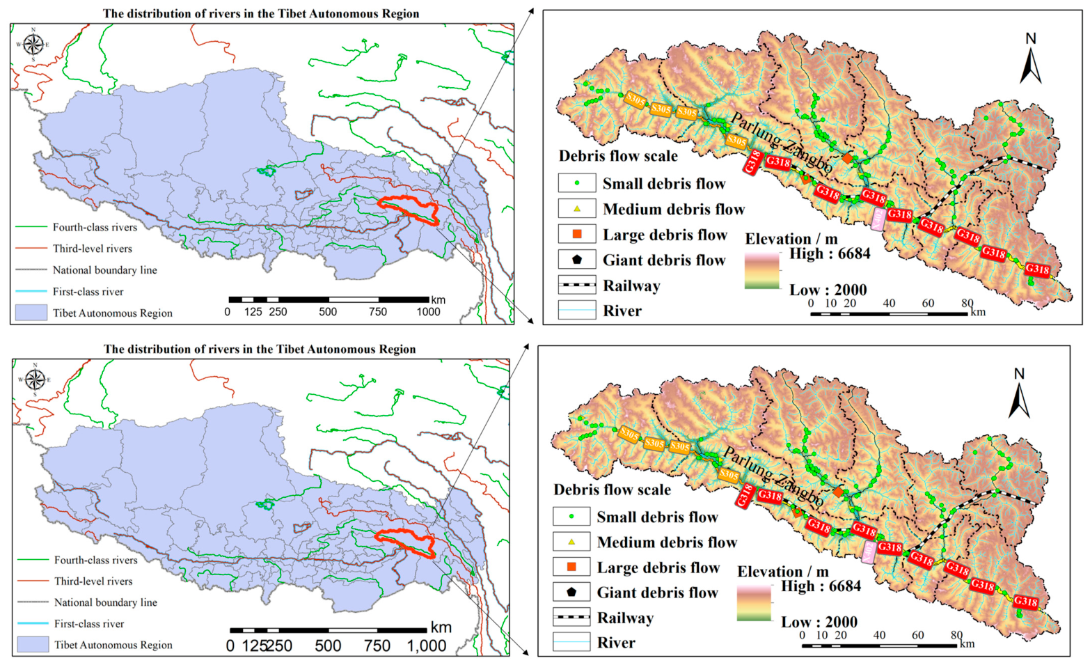
Bomi County is located in the southeastern part of the Tibet Autonomous Region, China. The study area spans from 94°04′05″ E to 96°39′12″ E longitude and 29°21′35″ N to 30°40′25″ N latitude under the WGS84 coordinate system. The region covers a total area of 16,767.91 square kilometers. It shares administrative boundaries with Basu County to the east, Luolong and Bianba Counties to the north, Jiali and Gongbujiangda Counties to the west, and Zayu County, Motuo County, and Bayi District to the south. Figure 1 illustrates the geographical position and regional context of the study area. From a geomorphological and hydrological perspective, Bomi County occupies the core region of the Parlung Zangbo River basin, a primary tributary of the Yarlung Zangbo River. The area lies at the southeastern margin of the Tibetan Plateau, a transitional zone characterized by significant topographic relief and tectonic uplift. The Parlung Zangbo basin features deeply incised valleys and acts as a moisture conduit for the Indian Ocean monsoon. Consequently, this basin configuration controls the regional drainage network and provides abundant oceanic glacial meltwater and concentrated precipitation. This combination of basin topography and climatic conditions creates an active environment for gravity-driven debris flows.
From a geomorphological and hydrological perspective, Bomi County occupies the core region of the Parlung Zangbo River basin, a primary tributary of the Yarlung Zangbo River. The study area lies at the active southeastern margin of the Tibetan Plateau, a transitional zone exhibiting significant topographic relief and tectonic uplift. The Parlung Zangbo basin features deeply incised valleys and serves as a moisture conduit for the Indian Ocean monsoon. Consequently, this basin configuration controls the regional drainage network and sustains abundant oceanic glacial meltwater and concentrated precipitation. This combination of steep topography and monsoonal climatic conditions facilitates frequent large debris flows.
Situated in the transitional belt between the South Tibet Valley of the Tibetan Plateau and the Hengduan Mountains, the region features rugged terrain characterized by steep mountain ranges and deeply incised valleys [43]. The Yigong Zangpo and Palong Zangpo rivers form the primary hydrological network, flowing southeastward across the county. Elevations vary significantly across the landscape, ranging from approximately 1800 m to 6684 m above sea level. Relative relief commonly exceeds 2000 m and reaches a maximum elevation difference of 4684 m. This topographic configuration indicates the substantial structural incision of the regional landforms [39].
Geologically, the regional lithology consists predominantly of metamorphic and sedimentary rocks. Unconsolidated Quaternary deposits cover these bedrock units, providing solid source materials that elevate regional susceptibility to debris flows [11]. Bomi County experiences a temperate plateau monsoon climate with moderate humidity. The southwest monsoon and warm oceanic airflows from the Indian Ocean dictate regional meteorological patterns. The climate features mild summers and winters, short frost durations, and large diurnal temperature fluctuations. Annual precipitation averages 800 to 1200 mm and concentrates primarily during the summer months. Consequently, these focused precipitation episodes serve as primary triggers for mass wasting phenomena and localized debris flows [10].

2.2. Debris Flow Inventory

Historical observations indicate that these events concentrate in valley bottom and alluvial fan areas. For example, debris flows in 2018 and 2020 damaged local communities and regional transportation systems. This study documented 192 debris flow events across Bomi County. The inventory integrates high spatial resolution remote sensing imagery interpretation, historical observations, and extensive field surveys. The delimitation criteria focused on identifying initiation zones and topographic source areas, as these regions reflect the geomorphological conditions prior to failure. Within a spatial analysis software environment, researchers digitized these source areas as geometric polygons to capture their morphological boundaries. To align with raster format spatial modeling, the workflow extracted the geometric centroids of these source polygons, representing the 192 events as spatial point features.
The documented mass wasting events vary in magnitude. Standard geological engineering specifications define the scale of each debris flow based on the estimated total volume of solid material ( V ). The regional inventory comprises four quantitative categories: one giant event ( V 10 6   m 3 ), five large events ( 10 5   m 3 V < 10 6   m 3 ), ten medium events ( 10 4   m 3 V < 10 5   m 3 ), and 176 small events ( V < 10 4   m 3 ).
The compilation, dating, and classification of this inventory relied on data acquired from multiple sources. Local archives from the Bureau of Natural Resources and the Meteorological Bureau provided historical event dates and their corresponding hydraulic triggers. These records confirm that intense monsoonal rainfall of short duration or episodic glacial meltwater surges triggered the majority of the dated debris flows, including the events documented in 2018 and 2020. Survey reports conducted after the disasters directly supplied the volume classifications for historically documented events. For undocumented events, interpreting remote sensing imagery across multiple time periods identified morphological changes. Additionally, geometric measurements of terminal depositional fans conducted in the field estimated the total volumes. An evaluation of development trends and activity levels classified these specific geomorphological sites. This assessment categorized 38 sites as relatively stable and 152 sites as stable, whereas the remaining two source areas exhibit active instability. DEMs of high spatial resolution enable the explicit characterization of these localized geomorphological features. Ultimately, these geospatial datasets provide the foundation for testing the proposed modeling strategy and generating susceptibility maps to support disaster risk mitigation and regional spatial planning.

2.3. Data Sources

This study integrated geospatial datasets from multiple sources to construct the debris flow susceptibility model. Primary data inputs include DEMs, regional geological maps, and land cover imagery. The workflow projected all spatial data into the WGS 1984 UTM Zone 46N coordinate system. Subsequently, the nearest neighbor interpolation algorithm resampled the datasets to a spatial resolution of 30 m. This standardization ensures spatial consistency across all data layers to support the reliable extraction of geomorphic features in raster format [20].
The United States Geological Survey (USGS) EarthExplorer platform provided the Advanced Spaceborne Thermal Emission and Reflection Radiometer Global Digital Elevation Model at a spatial resolution of 30 m. This raw dataset facilitated the extraction of macroscopic topographic variables, including slope, aspect, and profile curvature. Furthermore, the dataset yielded localized geomorphological indicators, such as surface roughness, local relief, flow accumulation, and the Topographic Position Index (TPI) [18]. Prior to feature extraction, spatial analysis software (ArcGIS version 10.8) applied a hydrological sink filling correction to the initial raster. This preprocessing step eliminates data voids and ensures accurate surface flow routing [4].
The China Geological Survey (CGS) provided a geological map at a scale of 1:200,000, which supplied regional lithology and fault system parameters. This study reclassified the original lithological units into engineering geological rock groups according to the mechanical strength, weathering degree, and structural integrity of the rock masses [11]. The data processing workflow digitized fault lines to compute the Euclidean distance to faults and fault density, providing quantitative proxies for rock mass fracturing and tectonic activity [2,11]. Additionally, geoprocessing algorithms derived the regional river network from the hydrologically corrected DEM to calculate the distance to rivers and drainage density. These indicators represent hydrological connectivity and the potential for basal toe erosion [27].
To assess surface resiliency, this study calculated the Normalized Difference Vegetation Index (NDVI) to quantify regional vegetation cover density, an ecological parameter influencing slope stability and soil erosion resistance [21]. Cloudless Landsat 8 Operational Land Imager (OLI) imagery, acquired during the peak vegetation growing season at a spatial resolution of 30 m, enabled the computation of NDVI values. Table 1 summarizes the spatial datasets, detailing their resolution, formats, and sources.
To construct the training dataset, this research applied a constrained negative background sampling strategy. Selecting negative points randomly across the study area often introduces spatial bias and misclassification in mountainous terrain. Therefore, the workflow generated negative samples selectively within geomorphologically stable zones exhibiting low topographic relief and minimal hydrological accumulation. This method provides an environmental contrast with the positive inventory, minimizes noise during the training phase, and enhances the boundary delineation capabilities of the ensemble model.
ArcGIS version 10.8 facilitated spatial data preprocessing, topographic feature extraction across multiple scales, and cartographic visualization. For subsequent algorithmic implementations, MATLAB R2021a and Python 3.8 programming environments executed the RF modeling and matrix computations to maintain computational efficiency.

3. Methodology

This section clarifies the theoretical boundary of the evaluation index system. This study evaluates debris flow susceptibility. Geographic frameworks define susceptibility as the spatial probability of occurrence resulting from inherent terrain conditions. This concept differs from hazard assessments, which additionally require the temporal probability of dynamic triggering mechanisms [45]. Consequently, the current spatial framework excludes dynamic hydrological and meteorological variables, such as transient rainfall sequences.
Spatial resolution constraints in alpine environments further explain the omission of dynamic rainfall inputs. Interpolating sparse regional meteorological data to a grid with a spatial resolution of 30 m introduces spatial uncertainty [46]. To compensate for the lack of direct rainfall data, this framework incorporates topographic proxies of high spatial resolution. Variables such as profile curvature, the TPI, and drainage line density parameterize the inherent hydrological routing potential, regional flow convergence, and localized drainage efficiency of hillslope units [47]. These static localized geomorphological indicators map how the terrain receives and redistributes potential hydrodynamic forces. This approach ensures the consistency of the spatial susceptibility assessment without requiring dynamic temporal inputs.

3.1. Selection of Evaluation Indicators

The interaction of geomorphological, geological, and hydrological parameters controls the occurrence of debris flows. Consequently, developing a systematic evaluation index system supports objective susceptibility mapping. This study selected conditioning factors by synthesizing field measurements in Bomi County, historical disaster records, and existing literature. These selected indicators represent the environmental characteristics of the study area. To structure the evaluation process, this research categorizes the conditioning factors into three thematic groups. These groups comprise macroscopic topographic indicators, localized geomorphological indicators, and geological environmental indicators.

3.1.1. Topographic Indicators

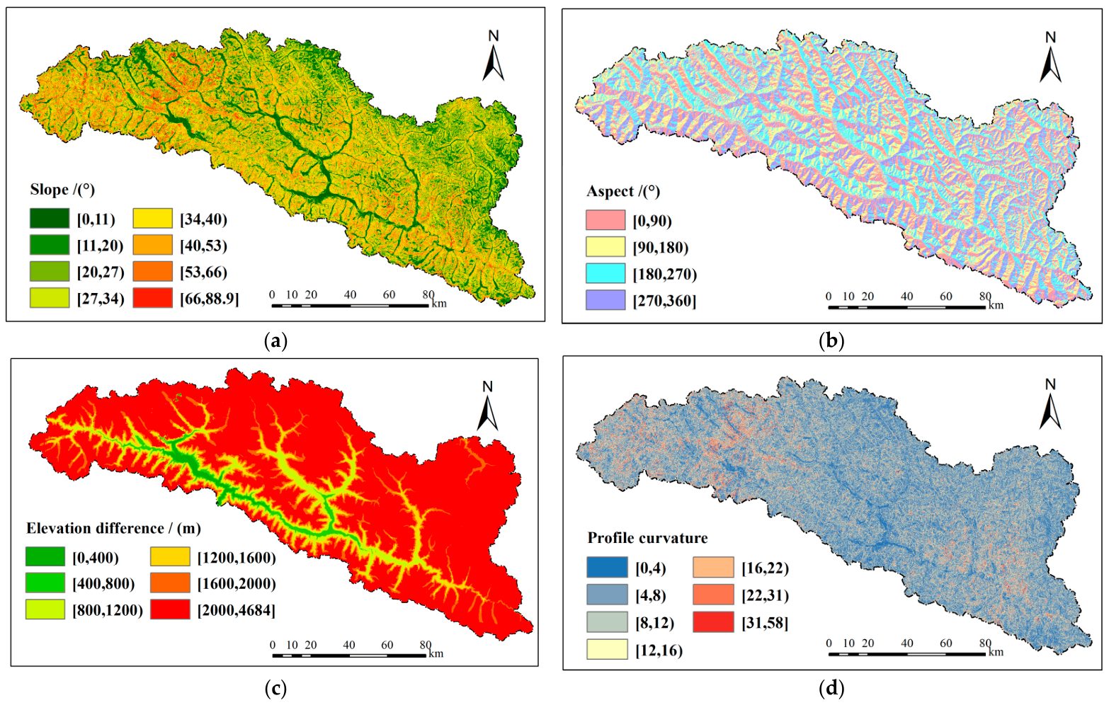
Topographic indicators derived from the ASTER GDEM at a spatial resolution of 30 m represent macroscopic terrain characteristics controlling gravitational potential energy and surface runoff processes. Rather than reviewing fundamental topographic principles, this framework focuses strictly on their physical contributions to debris flow initiation in Bomi County. Slope directly governs the mechanical erosion and sediment supply, reclassified into nine categories (Figure 2a). Aspect modulates local weathering rates and soil moisture, categorized into four classes (Figure 2b). Relative relief dictates the conversion of potential energy into kinetic transport energy, divided into six categories (Figure 2c). Finally, profile curvature determines vertical runoff convergence and pore water pressure accumulation, classified into seven levels (Figure 2d).

3.1.2. Micro-Geomorphic Indicators

Macroscopic topographic variables dictate the gravitational structure of a catchment, whereas localized geomorphological variations govern the physical boundaries of debris flow kinematics, including material initiation, flow channelization, and terminal deposition. To capture this spatial heterogeneity, quantify sediment connectivity, and provide contextual inputs to the machine learning framework, this study extracted localized geomorphological indicators.
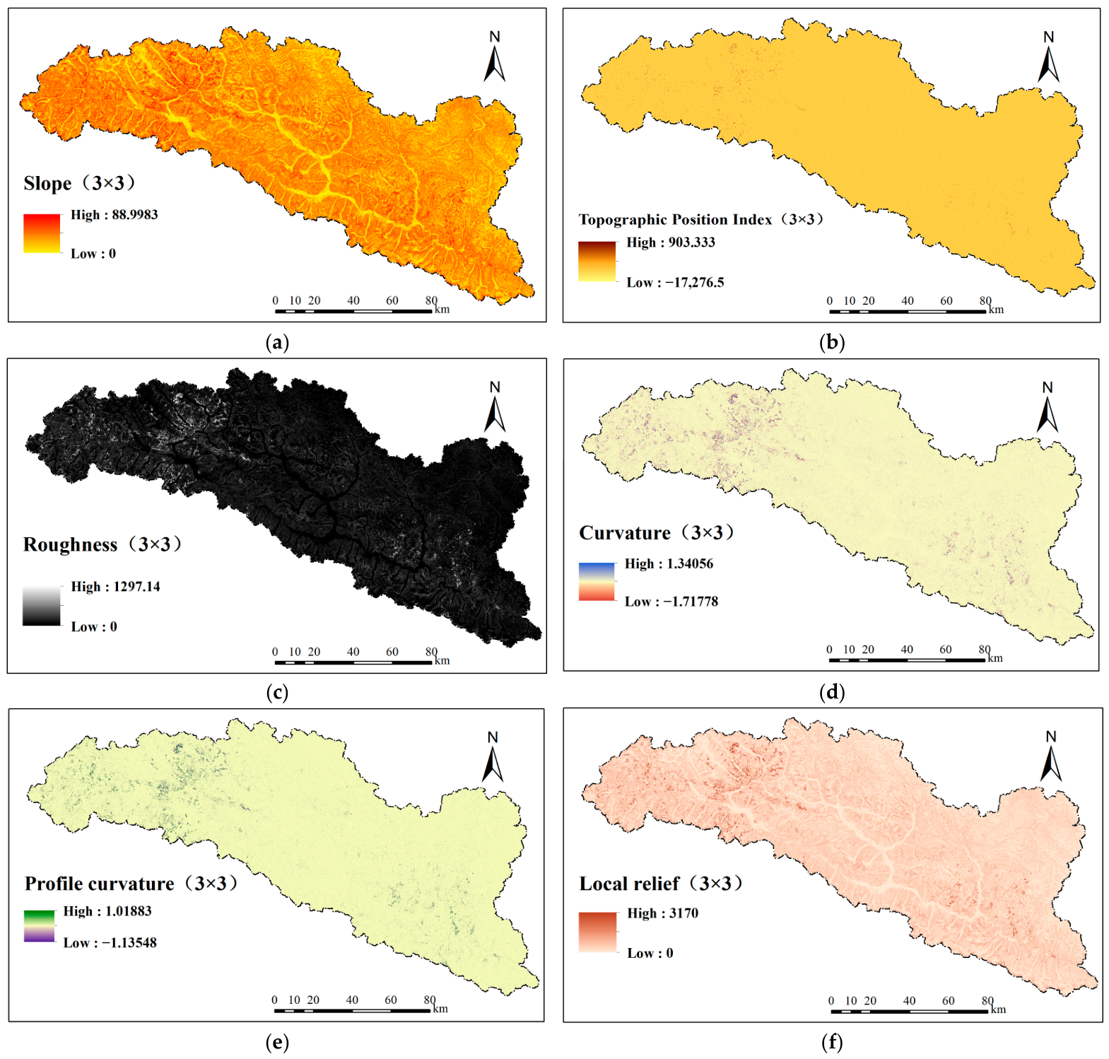
Instead of relying on a standard 3 by 3 pixel neighborhood, the computational extraction utilized moving windows across multiple scales to evaluate spatial sensitivity and capture regional hydrodynamic connectivity. Derived from the DEM of high spatial resolution, these parameterized indicators evaluate localized shear stress concentration, hydraulic convergence, and the kinematic resistance of individual hillslope units. Figure 3 illustrates the spatial distribution of the six extracted localized geomorphological layers across the Bomi County study region.
The predictive framework integrates six continuous topographic variables representing the physical processes governing debris flow kinematics. Rather than detailing their fundamental geometric definitions, this study emphasizes their direct parameterization of mass wasting mechanics. Slope (Figure 3a) and local relief (Figure 3f) govern gravitational shear stress and potential energy availability. The Topographic Position Index (TPI) differentiates localized landform positions (Figure 3b), while roughness acts as the numerical proxy for kinematic resistance (Figure 3c). Total and profile curvatures delineate regional flow convergence and runoff acceleration, controlling pore water pressure accumulation (Figure 3d,e).
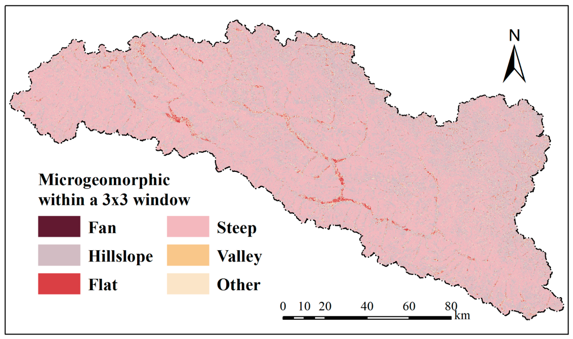
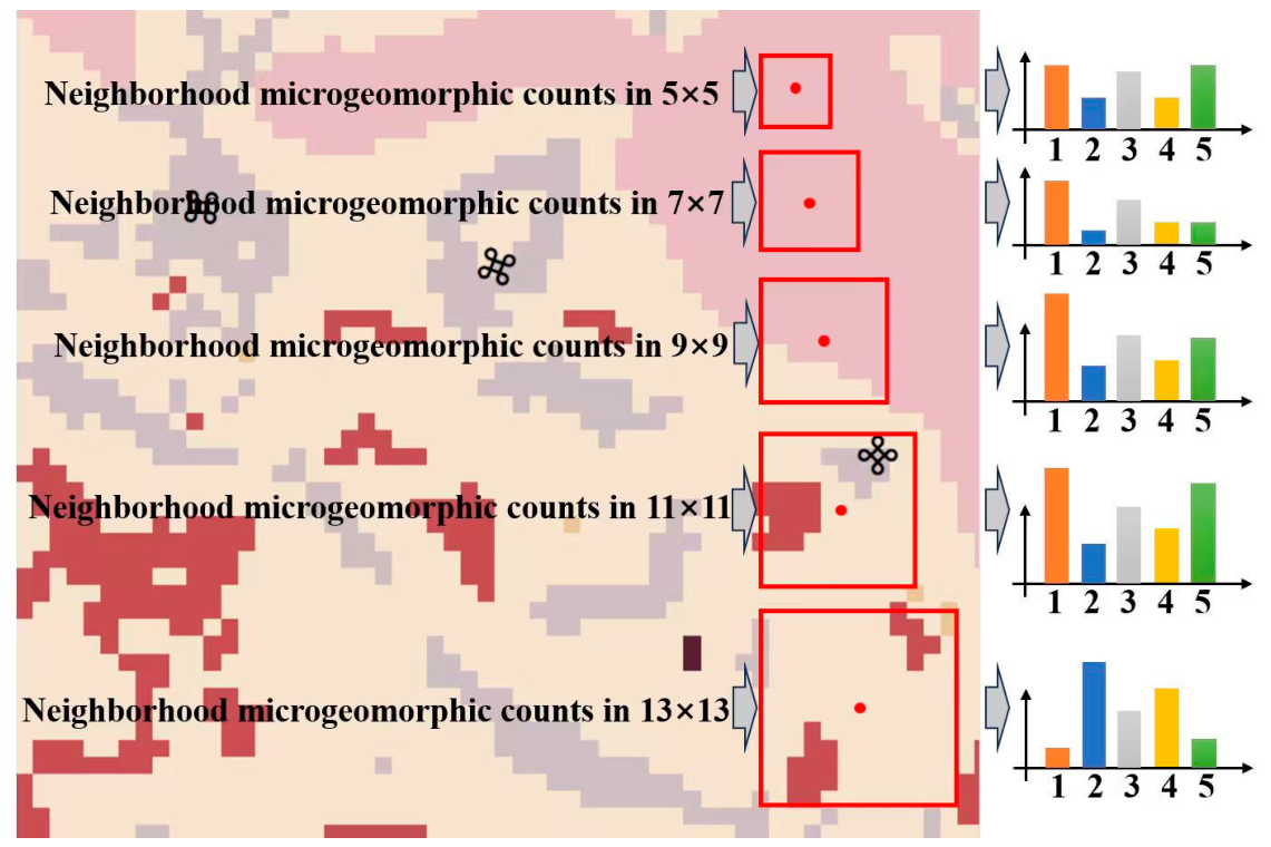
To bridge the conceptual gap between geometric variables and physical processes, this study synthesized these indicators into five discrete localized geomorphological process domains: fan, hillslope, flat, steep, and valley. The physical limits and mathematical interactions among slope, TPI, and curvature dictate this classification, providing a semantic map of the landscape (Figure 4). Subsequently, focal statistics algorithms executed a secondary spatial assembly. By calculating the frequency of each domain within progressively growing neighborhoods of 5 by 5 to 13 by 13 pixels, the spatial analysis quantified the adjacency and sediment connectivity between source hillslopes and transport valleys (Figure 4). This aggregation across multiple scales provides the downstream algorithms with contextual information, allowing the assessment of a single pixel alongside the interactive environment of the entire hillslope unit.
Each classified domain serves a specific functional role in the debris flow evolution cycle. Steep and hillslope domains act as primary material provenance zones where physical weathering ensures a continuous sediment supply. Valley areas serve as hydrodynamic routing corridors where runoff concentration fluidizes debris masses. Fan sections function as primary depositional and runout zones, whereas flat regions represent morphologically stable background contexts that inhibit mass wasting initiation.
The spatial arrangement of adjacent landforms governs the continuous process of debris flow routing. To digitize this geomorphological context, the methodology applied a secondary spatial filter to the discrete zonation maps. A focal statistics algorithm determined the occurrence frequency for each of the five localized geomorphological zones within expanded local neighborhoods, as shown in Figure 4.
The spatial analysis evaluated five progressively increasing statistical scales, ranging from 5 by 5 to 13 by 13 pixels. The red bounding boxes in Figure 5 denote the spatial extents of these sliding statistical windows, and the corresponding bar charts illustrate the quantitative frequency of landform assembly within each scale. These neighborhood assembly indicators provide contextual insights for the machine learning model. Consequently, the framework evaluates the individual landform condition of a central pixel alongside its physical interaction with the surrounding dynamic geomorphology.

3.1.3. Geo-Environmental Indicators

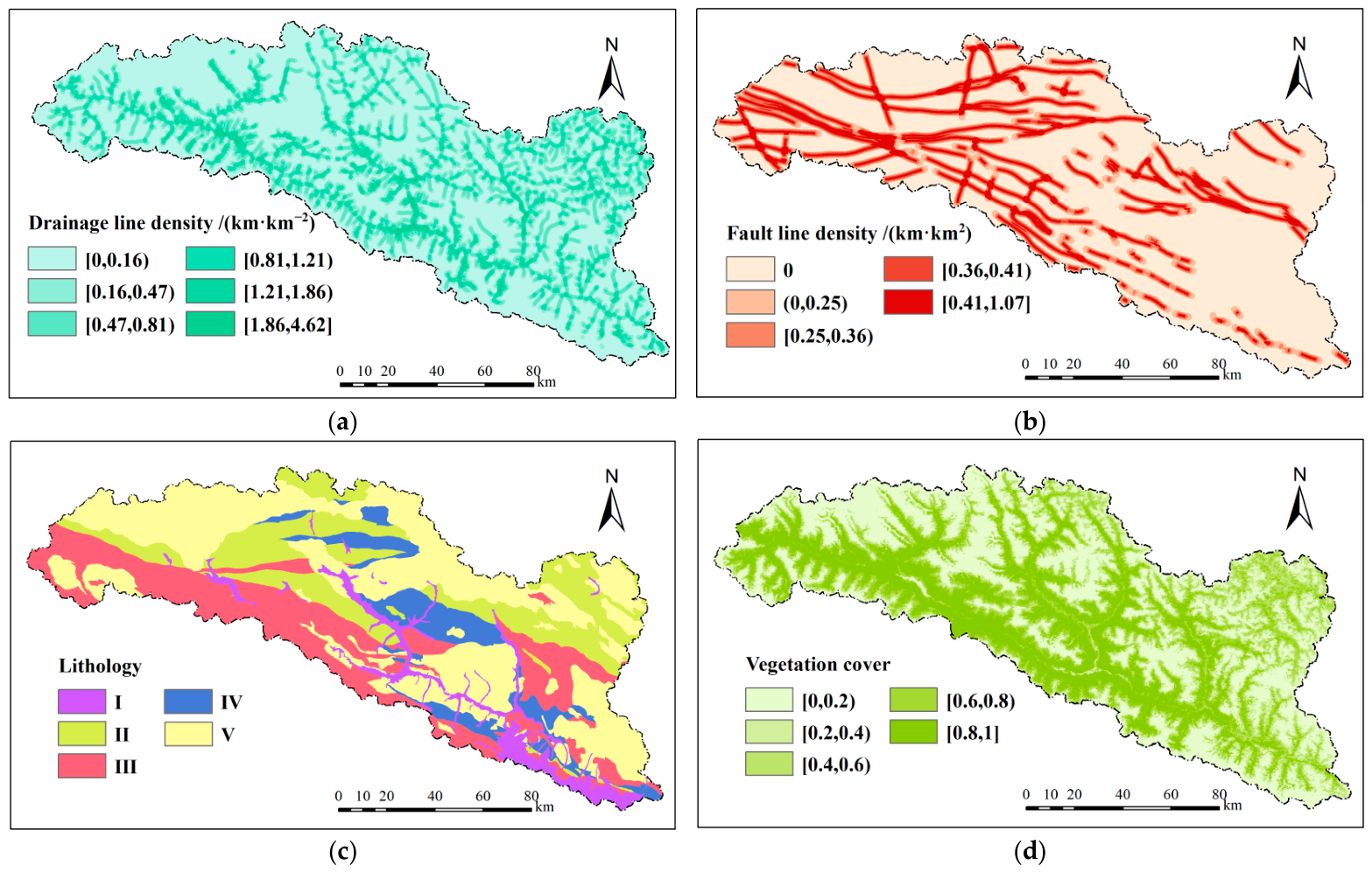
Geological environmental indicators represent the boundary conditions that counteract or facilitate debris flow initiation. To avoid redundant descriptions of fundamental geological mechanisms, this framework focuses strictly on their spatial parameterization. Drainage line density, which quantifies surface runoff convergence and fluvial erosion potential, was classified into six categories (Figure 6a). Fault line density reflects regional tectonic instability and rock mass fracturing, divided into five levels (Figure 6b). Vegetation cover, represented by the Normalized Difference Vegetation Index (NDVI), modulates surface stability and runoff interception. The spatial analysis classified this vegetation index into five levels (Figure 6d).
Furthermore, lithology controls the availability of loose source materials based on structural integrity and weathering resistance. Rather than exhaustively listing individual rock types, this study consolidated the lithological units into five primary engineering groups (Figure 6c): (I) unconsolidated sediments including sandy gravel and clay covering 1115.07 km2; (II) clastic sedimentary rocks such as medium to fine grained sandstone and mudstone spanning 3358.61 km2; (III) metamorphic rocks including quartzite and slate over 3920.34 km2; (IV) carbonate rocks such as fine to medium coarse textured marble and limestone across 1554.39 km2; and (V) intrusive igneous rocks, predominantly fine to medium coarse grained granite and diorite, representing the largest exposed area of 6819.50 km2.
Geomorphological and topographic derivatives, including slope, local relief, curvature, roughness, and the TPI, exhibit mathematical linkages and collinearity. To ensure the statistical independence of these multidimensional spatial arrays and the reliability of the variable importance evaluation, the workflow executed a correlation analysis prior to model training.
The Pearson correlation coefficient r quantified the pairwise linear relationships among all continuous spatial variables. The methodology set a correlation threshold of 0.7 to identify correlated feature pairs. Furthermore, the analysis calculated the Variance Inflation Factor (VIF) for each variable to assess global multicollinearity. The workflow flagged variables demonstrating a VIF value exceeding 10 as redundant and evaluated them for exclusion.
Although the RF ensemble architecture accommodates multicollinearity concerning overall predictive accuracy, extracting mathematically independent variables preserves the interpretability of the Mean Decrease Gini metric. Through these correlation constraints, the selected localized geomorphological variables provide independent information for the spatial predictive framework.
To process the continuous conditioning variables effectively, the methodology must account for the varied scales and distributions of the environmental datasets. Addressing the complexities of geohazard monitoring requires advanced protocols for automated normalizing large scale data. Consequently, this study recognizes the necessity of establishing a uniformly normalizing dynamic database across different topographical and hydrological factors. Techniques such as data normalization using piecewise symmetric functions provide a robust mathematical foundation for this preprocessing stage. This advanced normalization approach effectively mitigates the adverse effects of extreme spatial outliers and prepares the input matrices for potential dynamic filtering in subsequent temporal assessments.

3.2. Spatial Enhancement Analysis

Classical debris flow susceptibility models often treat individual grid cells as independent analytical units. This approach disregards spatial autocorrelation and the continuous nature of geomorphological processes. The interaction of neighboring terrains determines debris flow initiation and propagation. Localized morphodynamics govern the sediment supply and hydrological routing driving these processes. To represent this spatial heterogeneity, the methodology applied a spatial enhancement analysis across multiple scales using focal statistics and moving window algorithms.

3.2.1. Multi-Scale Moving Window Operations

The methodology applied moving window algorithms across multiple scales to implement the spatial enhancement proposed in Section 3.1.2. Omitting fundamental explanations of focal statistics, the workflow parameterized spatial scales into two logically nested sequences to capture both localized terrain fluctuations and regional sediment connectivity. First, the spatial analysis utilized construction windows ranging from 3 by 3 to 11 by 11 pixels to extract primary topographic features. Given the spatial resolution of 30 m for the underlying DEM, these matrices represent physical ground distances of 90 to 330 m, registering features from small rills to entire slope systems. Second, successive statistical windows assessed the spatial organization of the identified localized geomorphological regions. These windows possess a larger spatial footprint, spanning 5 by 5 to 13 by 13 pixels, corresponding to physical distances of 150 to 390 m. Setting the upper limit of the statistical windows higher than the construction windows allows the framework to measure the broader geomorphological context of localized central landforms.
To prevent spatial coordinate displacement during convolution across multiple scales, the spatial matrices strictly utilized sequences of odd numbers. Furthermore, a valid pixel masking algorithm embedded within the convolution functions prevented boundary propagation, recalculating the focal denominator using only valid neighboring pixels. These specific moving window operations maintain the spatial consistency of the study area boundary across all 25 scale combinations, ensuring exact pixel alignment during subsequent RF modeling.

3.2.2. Scale-Dependent Morphodynamics and Window Configurations

Following the moving window operations, the workflow incorporated the extracted spatial data into the machine learning structure to develop a sensitivity framework across multiple scales. The feature dataset introduces progressive statistical windows ranging from 5 by 5 to 13 by 13 pixels, each producing five quantitative spatial assembly indicators. These indicators represent the occurrence frequency of the fan, flat, hillslope, steep, and valley zones within a specific neighborhood. The methodology combined these localized assembly indicators with original continuous geological environmental variables, such as fault density and lithology, creating a spatial feature space of high dimensionality. Consequently, the RF algorithm assesses the individual physical features of the target site alongside the connectivity of surrounding sediments and topographic routing potential.
To evaluate the influence of spatial scales, the research applied a comprehensive combinatorial testing approach. The workflow combined five independent construction scales ranging from 3 by 3 to 11 by 11 pixels with five progressively expanding statistical scales ranging from 5 by 5 to 13 by 13 pixels, generating 25 unique spatial modeling scenarios. The workflow trained and tested the RF model separately on each configuration. Testing these progressively increasing windows captures the transition from localized geomorphological variation to macroscopic topographic smoothing. The analysis evaluated the predictive performance across these 25 scenarios using metrics such as the Area Under the Receiver Operating Characteristic Curve and the F score. This iterative evaluation automatically identifies the optimal threshold where the spatial connectivity of mass wasting landforms reaches a maximum prior to spatial averaging degrading the signal, effectively eliminating the scale subjectivity associated with traditional susceptibility evaluations.

3.3. RF Algorithm

T Breiman [58] proposed the RF algorithm, an ensemble machine learning method that constructs multiple decision trees during training. For debris flow susceptibility modeling, the RF algorithm processes spatial data of high dimensionality alongside nonlinear geological environmental variables. Furthermore, the RF architecture manages the multicollinearity present in spatial datasets [59]. This ensemble bagging design resists overfitting, addressing a limitation of conventional individual tree modeling methods.

3.3.1. Mathematical Formulation and Bagging Mechanism

The RF algorithm operates on the principles of Bootstrap Aggregating (Bagging) and random feature selection. Let the original training dataset be defined as S = { ( x i , y i ) } i = 1 N , where x i represents the multi-dimensional vector of the evaluation indicators (e.g., TPI, slope, lithology, precipitation) for the i -th spatial grid cell, and y i { 0 , 1 } denotes the absence or presence of a historical debris flow.
The algorithm randomly generates K independent bootstrap samples from the original dataset S with replacement. For each bootstrap sample, an unpruned Classification and Regression Tree (CART) is grown. To ensure diversity among the individual trees and reduce correlation, a random subset of m features is selected from the total M topographic and geo-environmental features at each node split (typically m M ).

3.3.2. Node Splitting Criterion

The optimal variable and threshold for splitting at each node are determined by minimizing the node impurity. In this classification task, the Gini Impurity is utilized as the splitting criterion [60]. The Gini Impurity I G ( p ) for a given node p is mathematically expressed as:
I G ( p ) = 1 i = 1 C ( p i ) 2
where C is the total number of classes (in this binary susceptibility assessment, C = 2 ), and p i is the empirical probability of an observation belonging to class i within that specific node. The algorithm selects the feature and the split point that maximize the decrease in Gini Impurity (i.e., information gain) between the parent node and the resulting child nodes.

3.3.3. Ensemble Prediction and Susceptibility Mapping

Once all K decision trees are constructed, the final susceptibility prediction for a given spatial grid cell x is determined by aggregating the predictions of the individual trees through majority voting:
H ( x ) = arg max c k = 1 K I ( h k ( x ) = c )
where H ( x ) is the final ensemble classification, h k ( x ) represents the prediction of the k -th tree, and I ( ) is the indicator function. For continuous susceptibility mapping, the proportion of trees voting for the “debris flow presence” class is extracted as the spatial susceptibility probability, ranging from 0 (very low susceptibility) to 1 (very high susceptibility).

3.3.4. Feature Importance Evaluation

The RF algorithm quantifies the predictive contribution of each evaluation indicator using the Mean Decrease Gini metric. Rather than detailing the standard calculation of impurity reduction across tree nodes, this study applies the resulting weight matrix to identify the primary mechanisms driving slope instability. Recent machine learning research emphasizes sensitivity analysis for predictive models [61,62]. To establish a rigorous sensitivity analysis framework, this study implemented a structured feature weight database. The generation method for these weights relies on the out of bag permutation technique. During the training phase of the ensemble model, the values of each conditioning variable are randomly permuted, and the corresponding decrease in predictive accuracy is recorded. This accuracy reduction serves as the raw sensitivity metric. For storage, these continuous importance metrics are compiled into a multidimensional array structure, ensuring that spatial identifiers and corresponding weight values are strictly linked and preserved for each algorithmic iteration. Regarding utilization, this database dynamically informs the feature selection process. Variables falling below a predefined importance threshold are systematically excluded from the final predictive framework, thereby optimizing model calibration, preventing computational redundancy, and maximizing overall predictability. Extracting these feature importance weights mitigates the black box dilemma and validates the physical mechanics of the susceptibility framework. By rejecting the equal likelihood assumption, this assessment directly verifies the unequal roles of localized geomorphological zones and their scale effects in the evolution of debris flows in Bomi County.

3.3.5. Parameter Optimization and Robustness Validation

To ensure the robustness and optimal performance of the debris flow susceptibility model, the workflow implemented a rigorous hyperparameter tuning protocol. Predictive optimality strictly depends on two primary hyperparameters: the total number of decision trees (ntree) and the number of features randomly sampled at each node split (mtry). A grid search strategy paired with tenfold cross validation determined the final model configuration. The spatial analysis monitored algorithm convergence via the Out of Bag error rate, identifying the threshold where the error stabilizes at a horizontal asymptote.
Furthermore, to ensure experimental reproducibility and eliminate random sampling biases, the methodology incorporated a strict replication strategy. The workflow executed the random forest framework across 20 independent spatial iterations utilizing a globally fixed random seed. This approach facilitated statistical error analysis, confirming that the generated susceptibility boundaries remain stable and are not artifacts of stochastic variance.

3.4. Evaluation Metrics

Standard statistical appraisal measures evaluate the predictive accuracy and extrapolation capability of the debris flow susceptibility model [63]. The performance assessment relies on the confusion matrix. This matrix compares the ground truth, indicating the observed presence or absence of debris flows, against the predicted classification outputs of the model.

3.4.1. Statistical Classification Metrics

The confusion matrix is composed of four fundamental elements: True Positives ( T P ), True Negatives ( T N ), False Positives ( F P ), and False Negatives ( F N ) [58]. In the context of this study, T P represents the number of actual debris flow locations correctly predicted as high susceptibility, while T N represents stable, non-debris flow areas correctly classified as low susceptibility. Based on these components, four critical statistical metrics were calculated: Accuracy, Precision, Sensitivity (Recall), and the F1-Score.
Accuracy represents the overall proportion of correctly classified grid cells relative to the total number of evaluated cells:
A c c u r a c y = T P + T N T P + T N + F P + F N
Precision measures the proportion of true debris flow locations among all grid cells that the model predicted as debris flows, reflecting the model’s ability to minimize false alarms:
P r e c i s i o n = T P T P + F P
Sensitivity (Recall) quantifies the proportion of actual debris flow locations that were correctly identified by the model, highlighting the model’s capability to prevent missed detections of critical hazards:
S e n s i t i v i t y = T P T P + F N
F1-Score is the harmonic mean of Precision and Sensitivity. It provides a single, balanced metric of model performance, which is particularly valuable when dealing with potentially imbalanced geospatial datasets:
F 1 S c o r e = 2 × P r e c i s i o n × S e n s i t i v i t y P r e c i s i o n + S e n s i t i v i t y

3.4.2. Receiver Operating Characteristic (ROC) Curve and AUC

Previous metrics evaluate model performance at specific thresholds, whereas the Receiver Operating Characteristic (ROC) curve provides an evaluation independent of these thresholds. Plotting the True Positive Rate (Sensitivity) on the vertical axis against the False Positive Rate on the horizontal axis across all classification thresholds constructs the ROC curve. The following equation defines the False Positive Rate:
F a l s e P o s i t i v e R a t e = F P F P + T N
The Area Under the Curve (AUC) quantifies the predictive accuracy of the ROC curve. The AUC value ranges from 0.5 to 1.0. A value of 0.5 indicates random classification, and a value of 1.0 denotes complete classification accuracy. Geospatial hazard modeling literature classifies AUC values between 0.7 and 0.8 as moderate, 0.8 to 0.9 as high, and greater than 0.9 as very high [64]. Consequently, the AUC provides an objective assessment of the spatially enhanced variables and localized geomorphological indices for classifying debris flow susceptibility across the study area.

3.4.3. Continuous Probabilistic Error Metrics

While confusion matrix attributes evaluate performance at specific classification thresholds, they omit continuous predictive variance. To provide an evaluation independent of thresholding, this study utilized two continuous probabilistic error metrics: Root Mean Square Error (RMSE) and Mean Absolute Error (MAE). These metrics strictly quantify the deviation between the continuous susceptibility probability outputs and the binary ground truth, directly measuring the average magnitude of predictive errors without relying on traditional thresholding equations. The following equation defines the MAE:
M A E = 1 N i = 1 N | P i O i |
The RMSE applies a quadratic penalty to larger prediction errors, making it highly sensitive to significant misclassifications. It is mathematically defined as:
R M S E = 1 N i = 1 N ( P i O i ) 2
Here, N represents the total number of evaluated spatial grid cells, P i denotes the continuous predicted susceptibility probability for cell i , and O i signifies the binary observation. Lower RMSE and MAE values indicate high probabilistic predictive accuracy and accurate calibration of the spatial model.

4. Results

4.1. Feature Importance Analysis

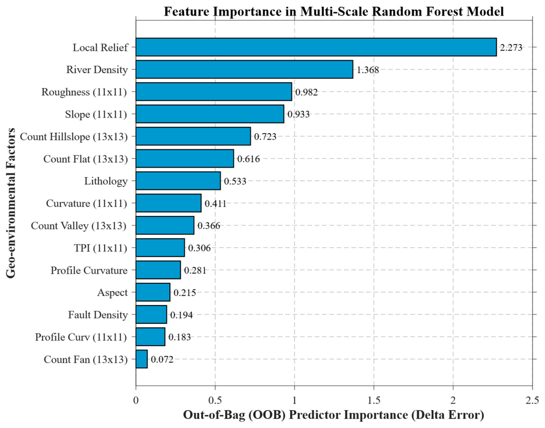
To identify the nonlinear causal factors underlying debris flows in Bomi County, the methodology executed a quantitative feature importance analysis. This analytical framework improves the physical interpretability of the RF model. The OOB Permuted Predictor Delta Error metric assesses the relative contribution of each geological environmental factor. This metric quantifies the decrease in predictive capability when the algorithm randomly shuffles the information related to a specific variable. A larger Delta Error value indicates an increased dependence of the model on that specific factor.
As Figure 7 shows, Local Relief constitutes the primary predisposing factor, achieving the highest importance score of 2.273. Within the incised alpine gorges of the southeastern Tibetan Plateau, local relief dictates the gravitational potential energy. Mass wasting processes utilize this energy as the primary dynamic driver initiating debris flows. River Density ranks second with a score of 1.368, underscoring the role of hydrodynamic forcing. Dense river networks facilitate surface runoff convergence to fluidize loose materials and intensify fluvial undercutting at slope toes. This process continually weakens adjacent hillslopes and supplies dynamic channel networks with solid source materials.
The ranking highlights the predictive contribution of the spatially enhanced localized geomorphological indicators. Computed over the optimal construction window, Roughness at an 11 by 11 pixel scale scores 0.982 to rank third, and Slope at the same scale scores 0.933 to rank fourth. This contribution confirms that debris flow kinematics depend on localized topographic features. Rather than processing raw individual pixel values, the focal statistics applied across the 11 by 11 window capture the morphological sharpening and shear stress concentrations of the slope elements while smoothing high frequency terrain noise.
Furthermore, the neighborhood assembly indicators based on the 13 by 13 statistical window demonstrate substantial predictive value. The importance scores of the Hillslope count indicator at 0.723 and the Flat count indicator at 0.616 evidence this capability. This result indicates the algorithm captures sediment connectivity. The model evaluates how the spatial arrangement of surrounding landforms, such as adjacent steep hillslopes supplying debris to the target unit, dictates the vulnerability of a specific site.
Lithology scores 0.533, functioning as an intermediate discriminating factor for the material foundation. The rock mass weathering rate depends on the presence of unconsolidated Quaternary sediments. Traditional macroscopic and structural variables, including Aspect with a score of 0.215 and Fault Density with a score of 0.194, occupy the lower end of the hierarchy. Although regional tectonic fracturing weakens rock masses, local topography gradients and hydrogeomorphological convergence control the triggering of individual debris flows in this alpine setting.
Ultimately, the physical significance of the feature importance hierarchy validates the proposed modeling framework across multiple scales. Integrating localized geomorphology and spatial connectivity allows the RF algorithm to describe earth surface processes with greater precision than conventional macroscopic indicators achieve.

4.2. Model Performance and Spatial Validation

To ensure accurate geological susceptibility mapping and prevent algorithmic overfitting, the methodology executed a spatial validation and cross validation strategy prior to performance evaluation. The data processing partitioned the historical geospatial debris flow inventory, allocating 70% to model training with an embedded tenfold cross validation protocol and reserving the remaining 30% as an independent testing dataset.
Using this isolated testing dataset, the analysis evaluated the predictive power, robustness, and scale sensitivity of the localized geomorphological RF framework across multiple scales. The evaluation involved a metric matrix of high dimensionality encompassing metrics independent of thresholds, such as the AUC, and statistical measures dependent on thresholds, including Accuracy, Precision, Recall, and the F1 score.
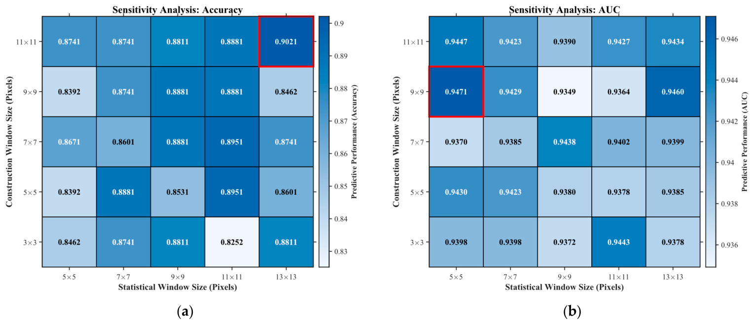
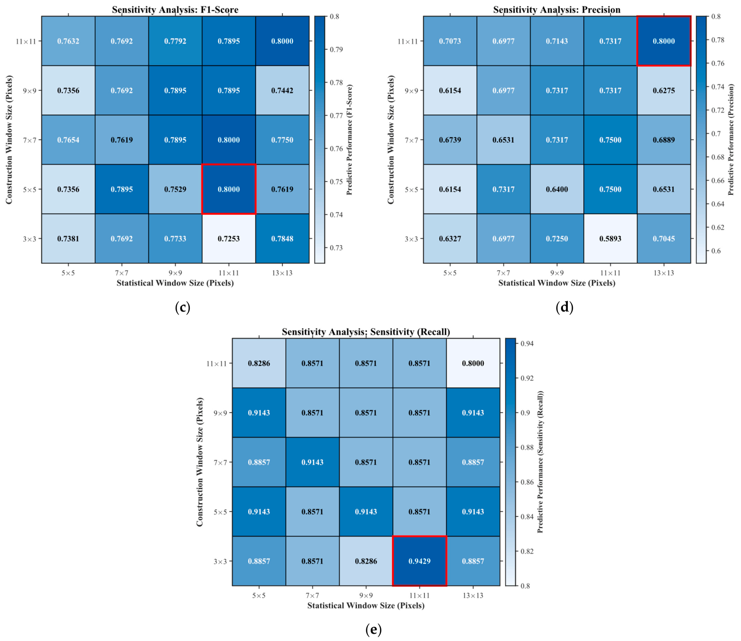
The spatially modified model demonstrated high classification accuracy during the spatial layout operation comprising an 11 by 11 extraction window and a 13 by 13 statistical window. On the independent 30% testing dataset, the model achieved a total accuracy of 90.21%. Furthermore, it recorded a precision of 0.8000, a recall of 0.8000, and a harmonic F1 score of 0.8000. Concurrently, the predictive power of the model independent of thresholds reached an AUC value of 0.9434.
This balanced performance profile facilitates viable geohazard mitigation. The recall of 0.8000 minimizes the omission error rate, indicating the model correctly identified active debris flow initiation corridors and runout channels. Simultaneously, the precision and F1 score of 0.8000 confirm the algorithm suppressed false positive alarms in background areas possessing similar morphological characteristics but higher stability, thereby preventing spatial overestimation. The mathematical convergence of precision and recall in this regional configuration demonstrates that parameterized localized geomorphology and sediment connectivity provide a precise and physically consistent representation of earth surface processes compared to conventional isolated pixel models.
Geomorphological processes controlling alpine debris flows exhibit scale dependence. Figure 8 and Table 2 illustrate the variation in the five evaluation measures across the 25 computational scenarios. Combining five construction windows, ranging from 3 by 3 to 11 by 11 pixels, with five statistical windows, ranging from 5 by 5 to 13 by 13 pixels, generated these scenarios.
The sensitivity matrix demonstrates the mathematical convergence of global performance measures. The spatial arrangement comprising the 11 by 11 construction window and the 13 by 13 statistical window records the peak Accuracy of 90.21 percent, a Precision of 0.8000, and an F1 score of 0.8000. This convergence across multiple metrics indicates that this regional assembly matches the physical attributes of the deeply incised gorges and sediment transport corridors in Bomi County. At this spatial scale, the operators capture sediment connectivity and local landform assemblies, including the spatial proximity of steep source slopes and downstream transport valleys, while excluding background noise.
The sensitivity matrices also reveal the limits of spatial enhancement across the landscape. The smallest spatial context, comprising the 3 by 3 construction window and the 5 by 5 statistical window, yields a baseline predictive performance. Under this localized constraint, the Precision decreases to 0.6327 and the F1 score drops to 0.7381. At this restricted scale, elevation model artifacts and high frequency topographic noise obscure terrain properties. Consequently, the limited spatial extent fails to capture the continuous hydrological and geomorphological gradients driving sediment movement.
Expanding the statistical window reveals the influence of feature context. For the 11 by 11 construction window, enlarging the statistical neighborhood from 5 by 5 to 13 by 13 pixels increases the F1 score from 0.7632 to 0.8000 and the Accuracy from 87.41 to 90.21 percent. This progression demonstrates that expanding the focal statistics operator enables the RF algorithm to resolve local geomorphological discontinuity. The 13 by 13 statistical window provides the spatial envelope to connect distinct process areas, establishing the transition boundaries between steep slope failures and low gradient deposition zones while preserving localized information.
Evaluating 25 combinations across multiple metrics eliminates the spatial scale bias present in traditional data driven assessments. This methodology aligns the machine learning architecture with the spatial characteristics of the local mass wasting environment.

4.3. Debris Flow Susceptibility Mapping

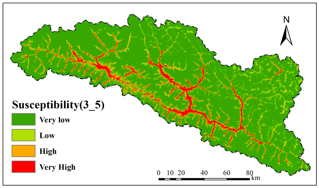
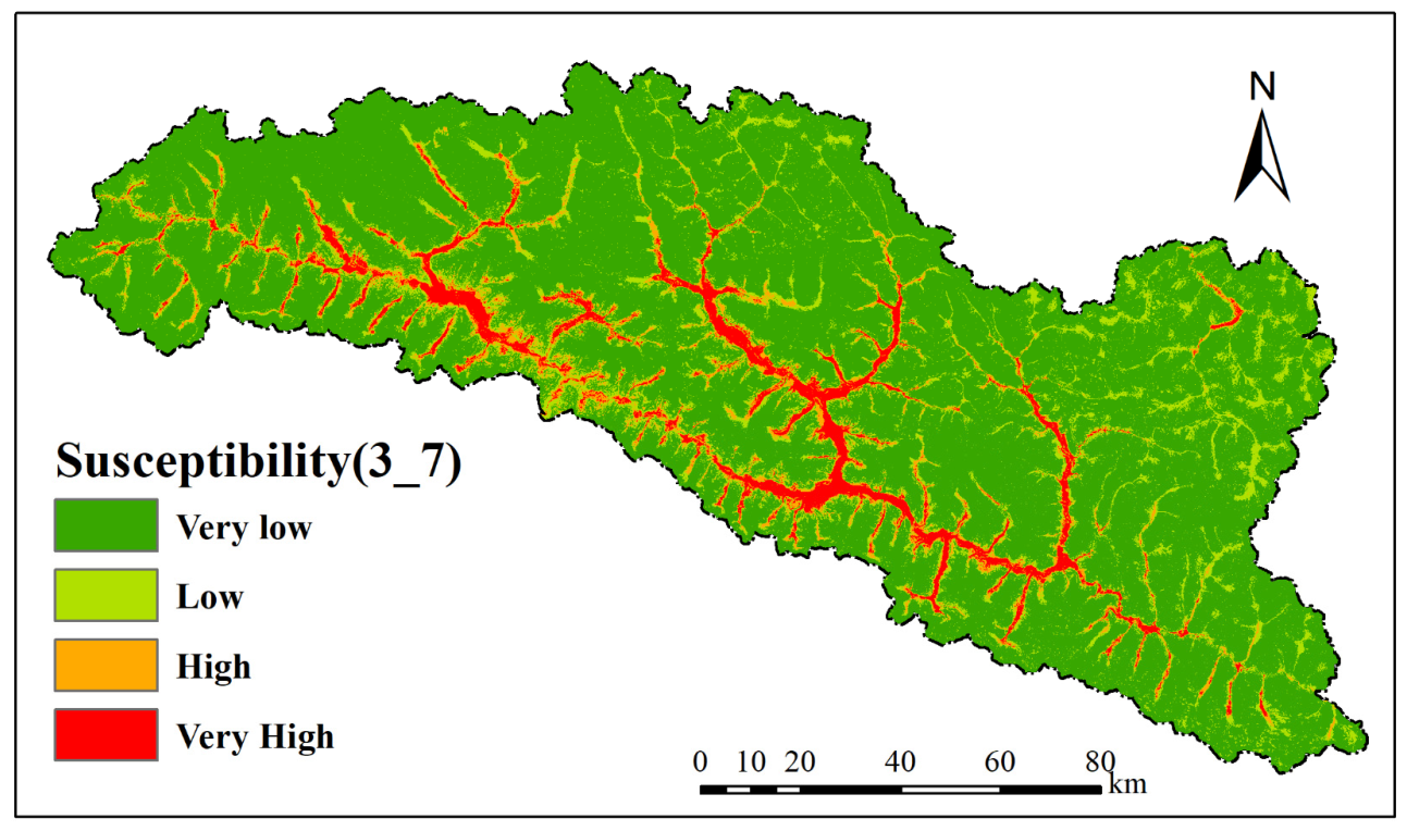
The mapping process extrapolated all 25 computational results across Bomi County to generate a spatial sensitivity atlas across multiple scales, as Figure 9 illustrates, prior to isolating the final hazard areas for engineering applications. The horizontal axis of this atlas depicts the expansion of the neighborhood statistical windows, progressing from 5 by 5 to 13 by 13 pixels. The vertical axis indicates the expansion of the localized geomorphological construction windows, progressing from 3 by 3 to 11 by 11 pixels.
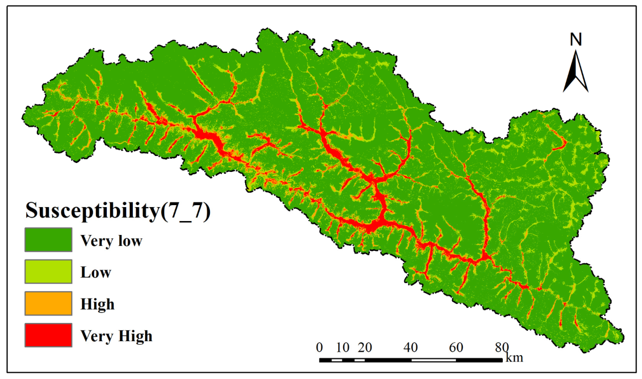
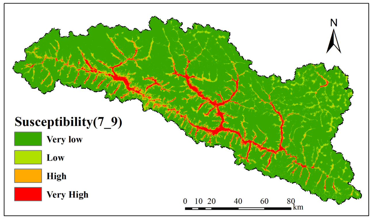
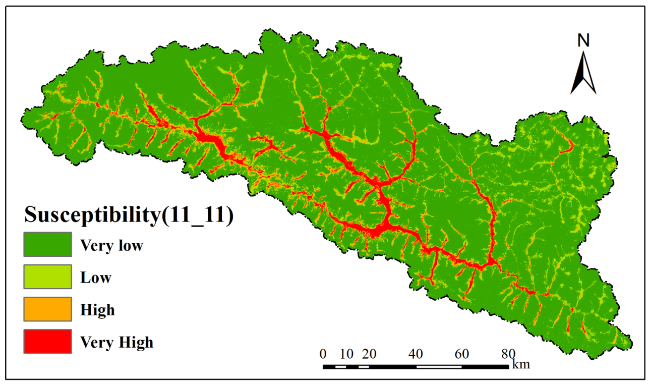
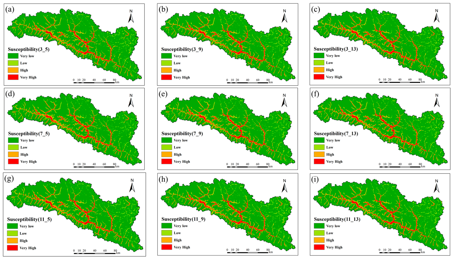
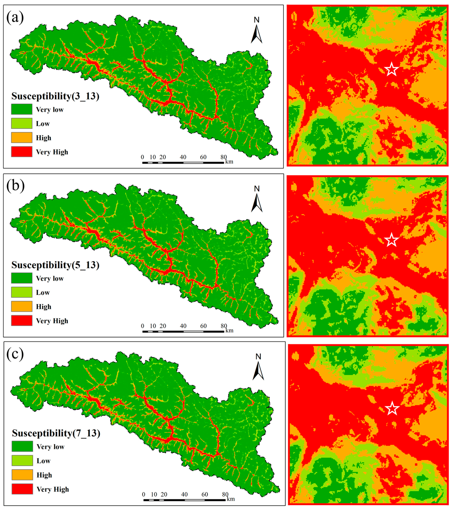
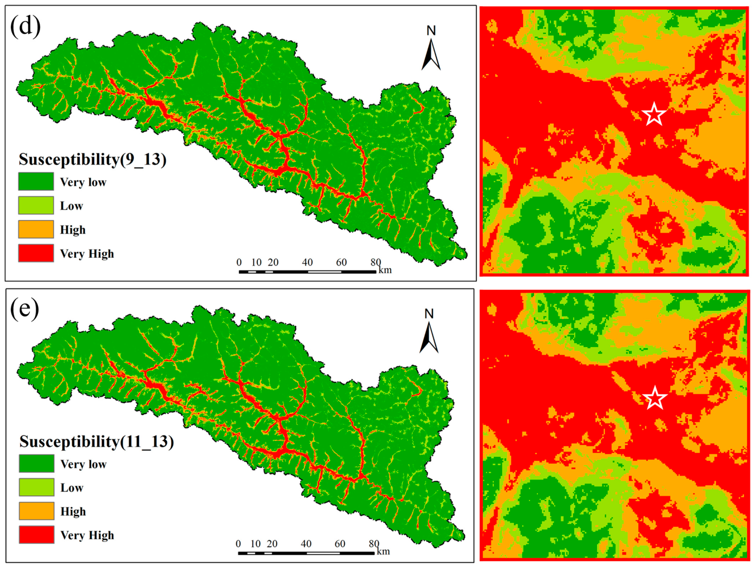
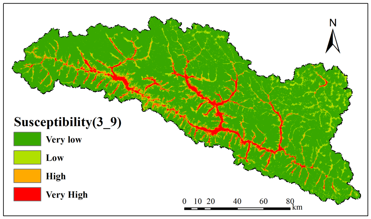
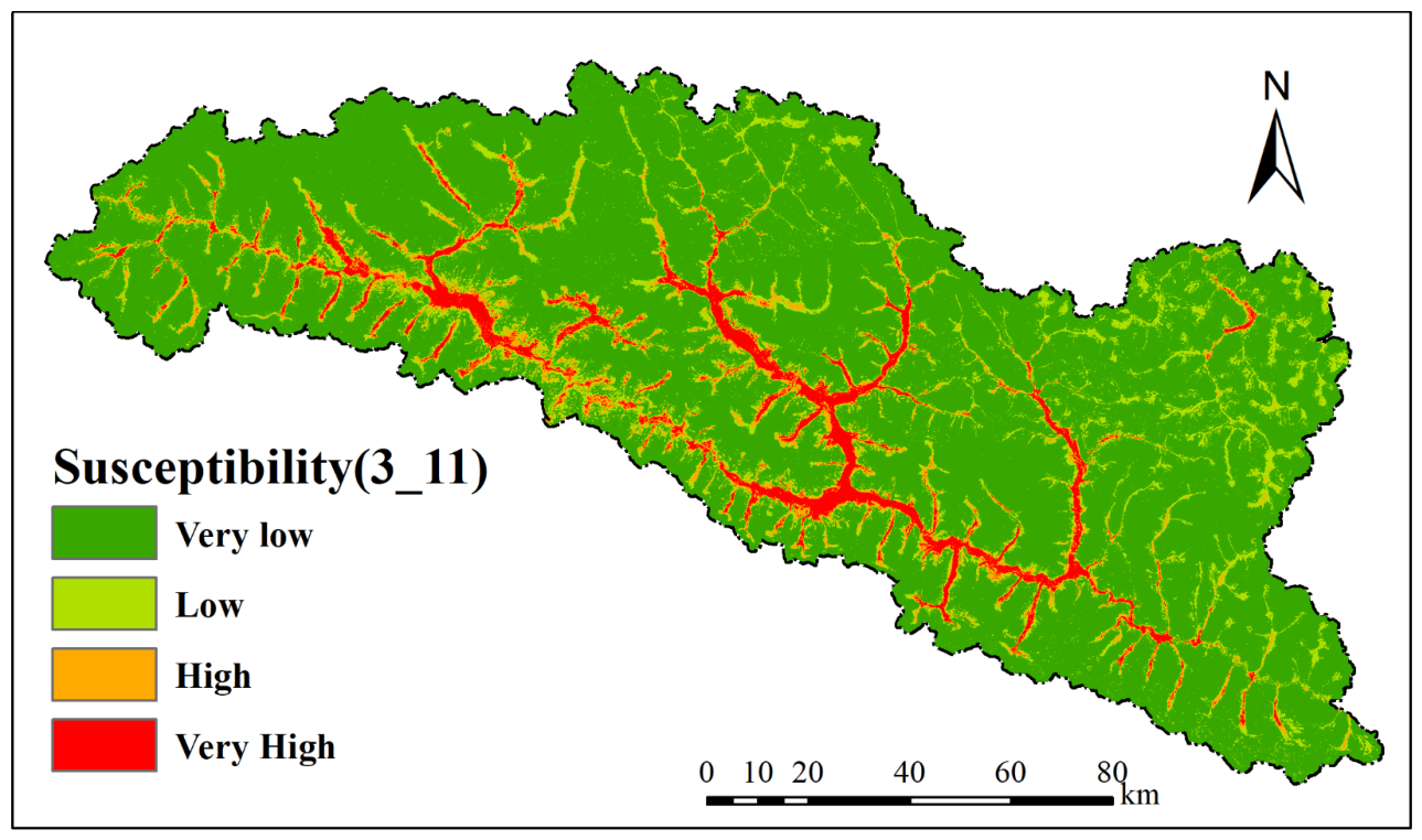
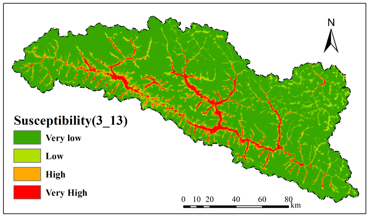
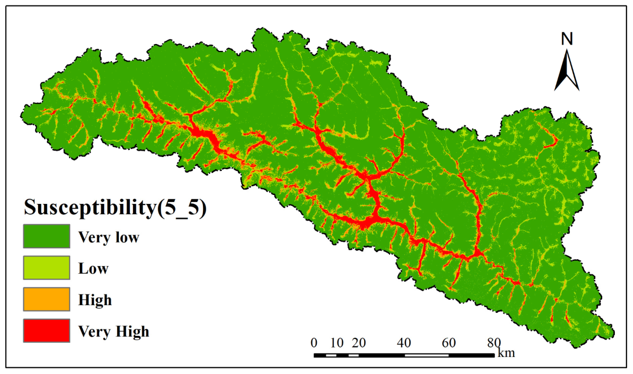
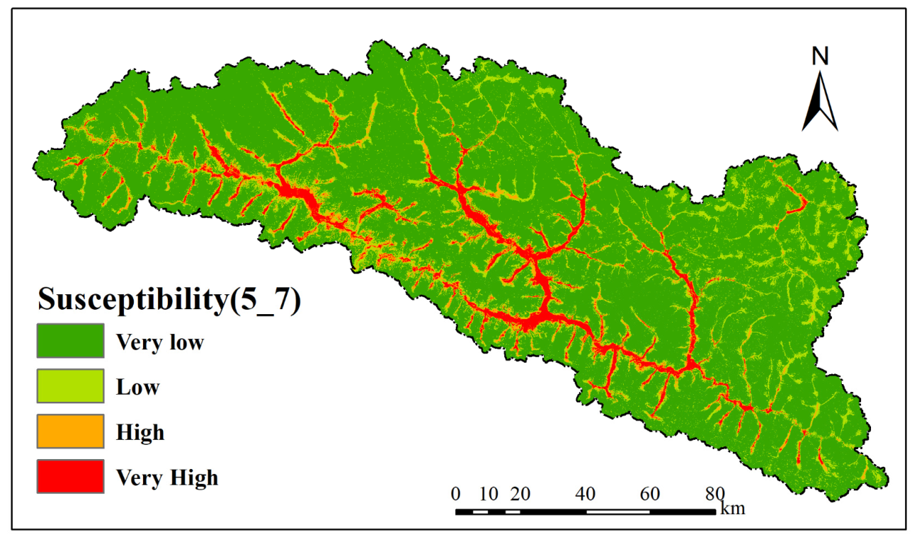
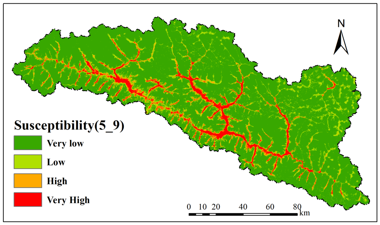
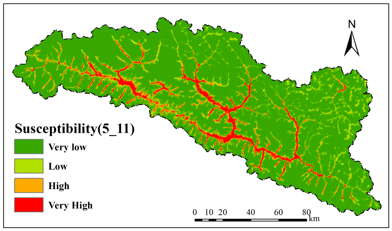
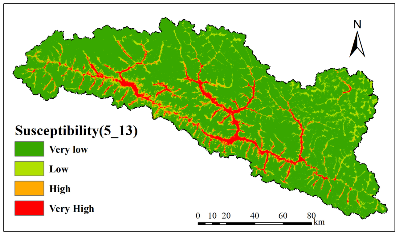
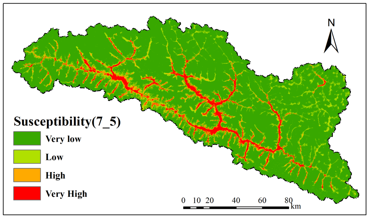
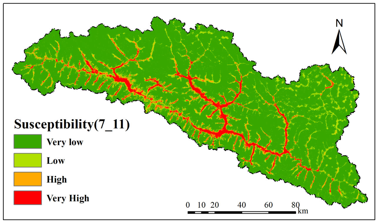
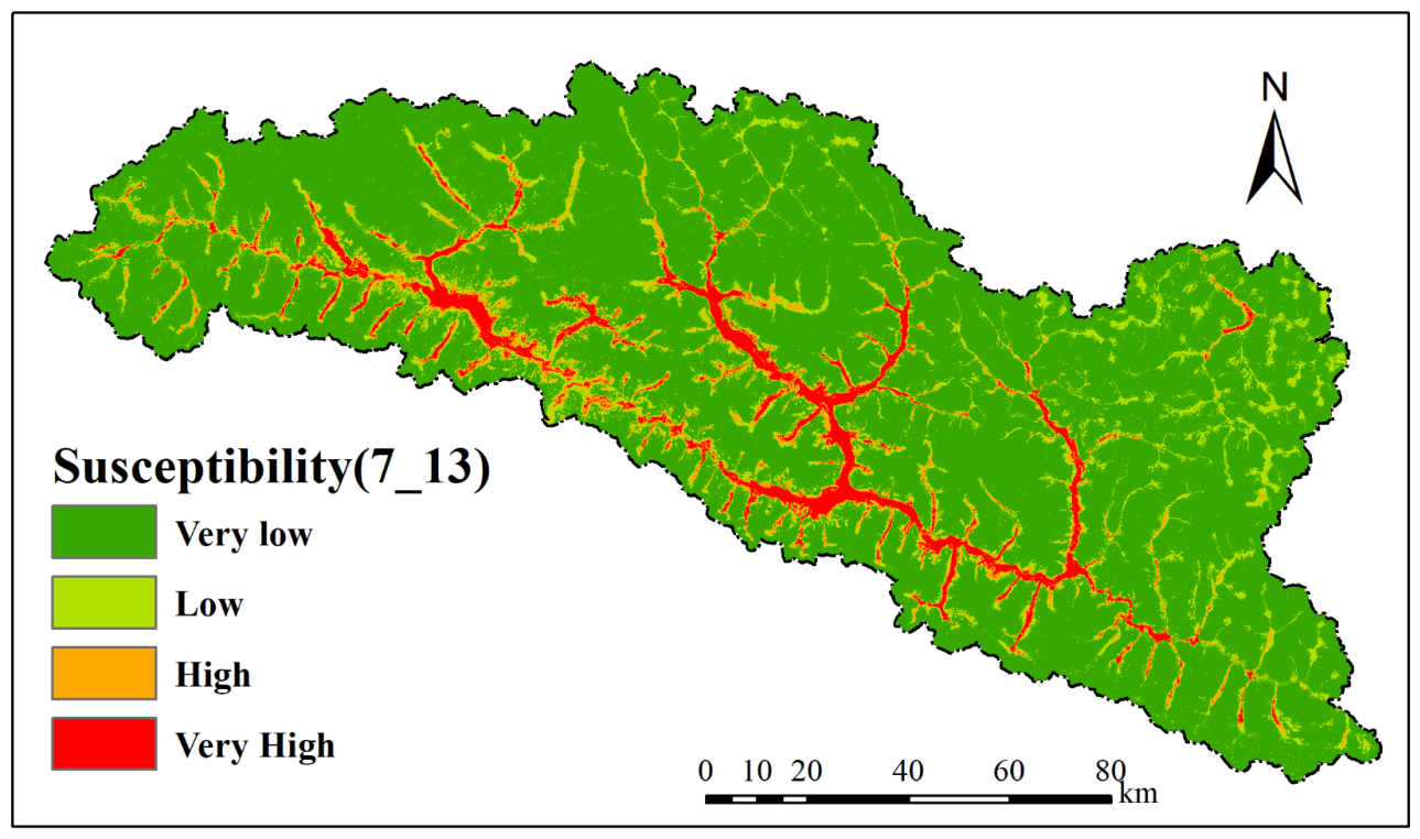
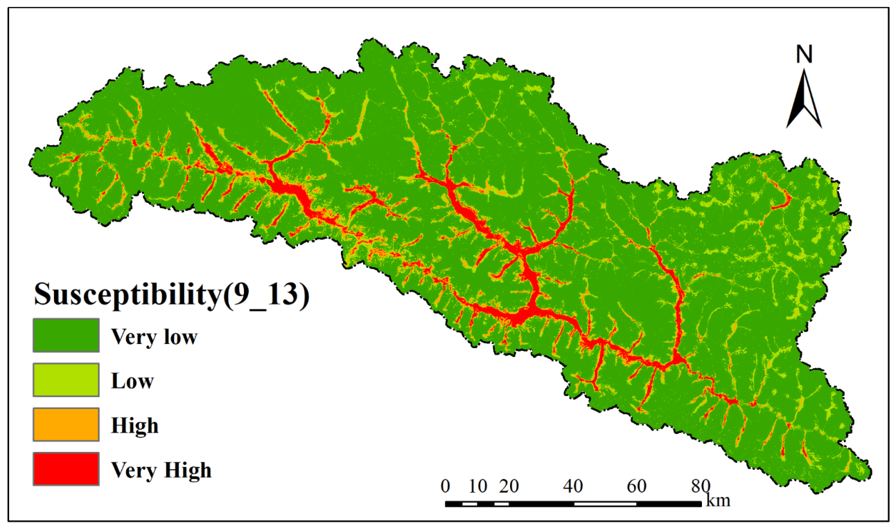
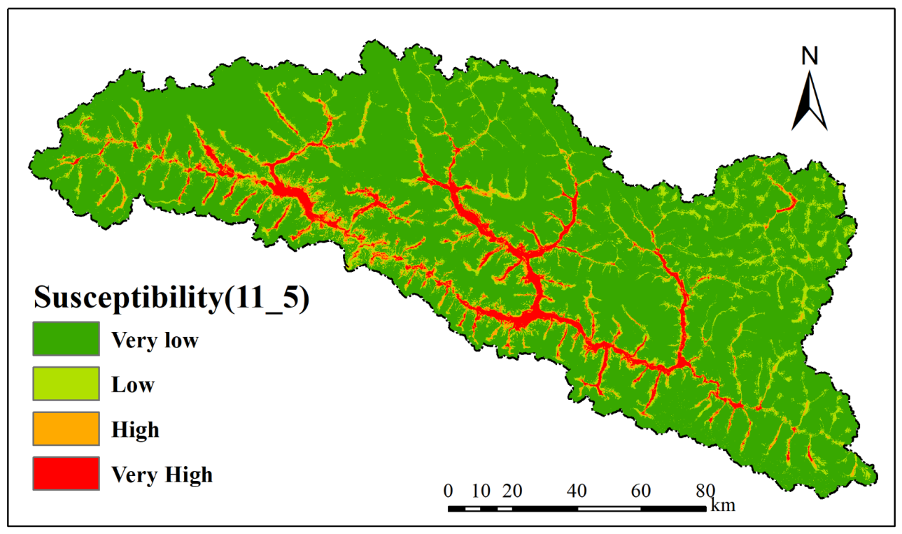
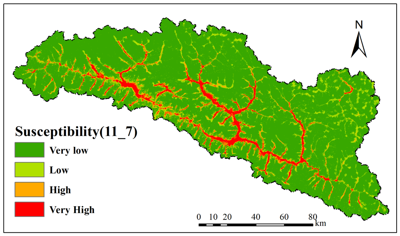
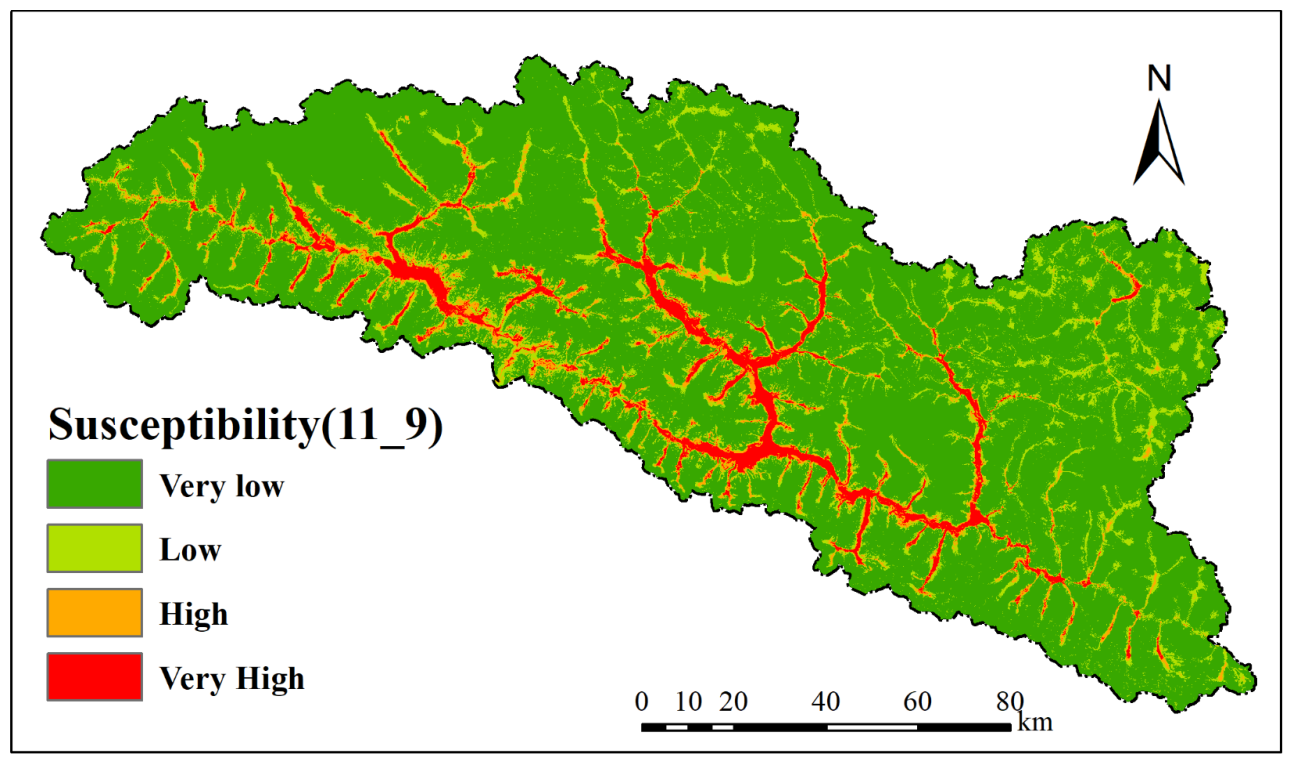
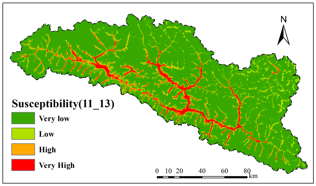
Visual examination of the 25 model grid (see Figure A1, Figure A2, Figure A3, Figure A4, Figure A5, Figure A6, Figure A7, Figure A8, Figure A9, Figure A10, Figure A11, Figure A12, Figure A13, Figure A14, Figure A15, Figure A16, Figure A17, Figure A18, Figure A19, Figure A20, Figure A21, Figure A22, Figure A23, Figure A24 and Figure A25 in Appendix A) reveals a structured cartographic progression. This progression corresponds directly with the quantitative metrics detailed in Section 4.2. Restrictive spatial combinations at the bottom left of the atlas generate susceptibility maps exhibiting extensive granular fragmentation. Topographic noise and DEMs artifacts produce disjunctive clusters of high risk pixels across geomorphologically stable planar plateau regions. Increasing the sliding matrix size toward the spatial arrangement of an 11 by 11 construction window and a 13 by 13 statistical window progressively reduces this topographic noise. The fragmented patches integrate into continuous and structurally coherent hazard corridors. This cartographic shift illustrates how the context aware neighborhood assembly algorithm resolves the isolated pixel limitation to capture continuous sediment routing pathways.
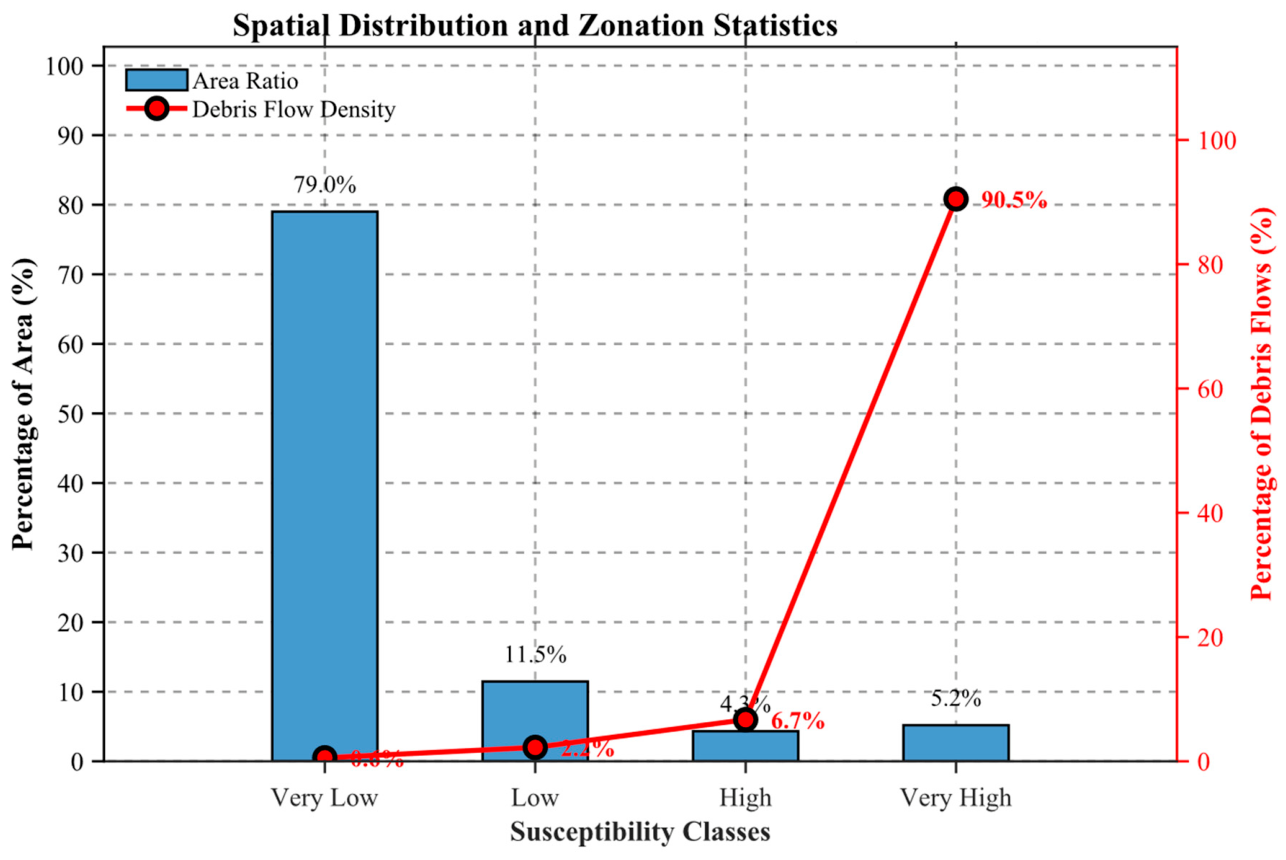
To address spatial uncertainties and validate the mapped outcomes, the spatial analysis overlaid the discretized susceptibility classes with the historical inventory of 192 documented debris flow events. A composite chart with dual axes depicts the relationship between the geographical area percentage of each susceptibility class and the geohazard hit ratio.
The empirical distribution indicates a skewed risk concentration. The Very High susceptibility zone occupies a minor geographic footprint within Bomi County. Within this spatial envelope, the hazard density curve reaches the global maximum, containing the majority of the recorded historical debris flows. Combining the Very High and High susceptibility categories restricts the risk to a prioritized zoning footprint, minimizing the omission error rate.
Conversely, the Very Low susceptibility class corresponding to the stable background terrain demonstrates the reverse statistical trend. This class encompasses the largest geographical percentage of the study area. However, the debris flow density curve approaches the global minimum and contains few historical disasters. This divergent trend across two dimensions, where hazard density increases as land area transitions to more susceptible strata, demonstrates the spatial discrimination and background noise suppression capabilities of the neighborhood assembly framework across multiple scales.
Figure 10 demonstrates that the scale configuration narrows the critical inspection zones. This spatial delineation provides civil authorities with data for early warning sensor network implementation and regional land use planning.

4.4. Impact of Spatial Scales

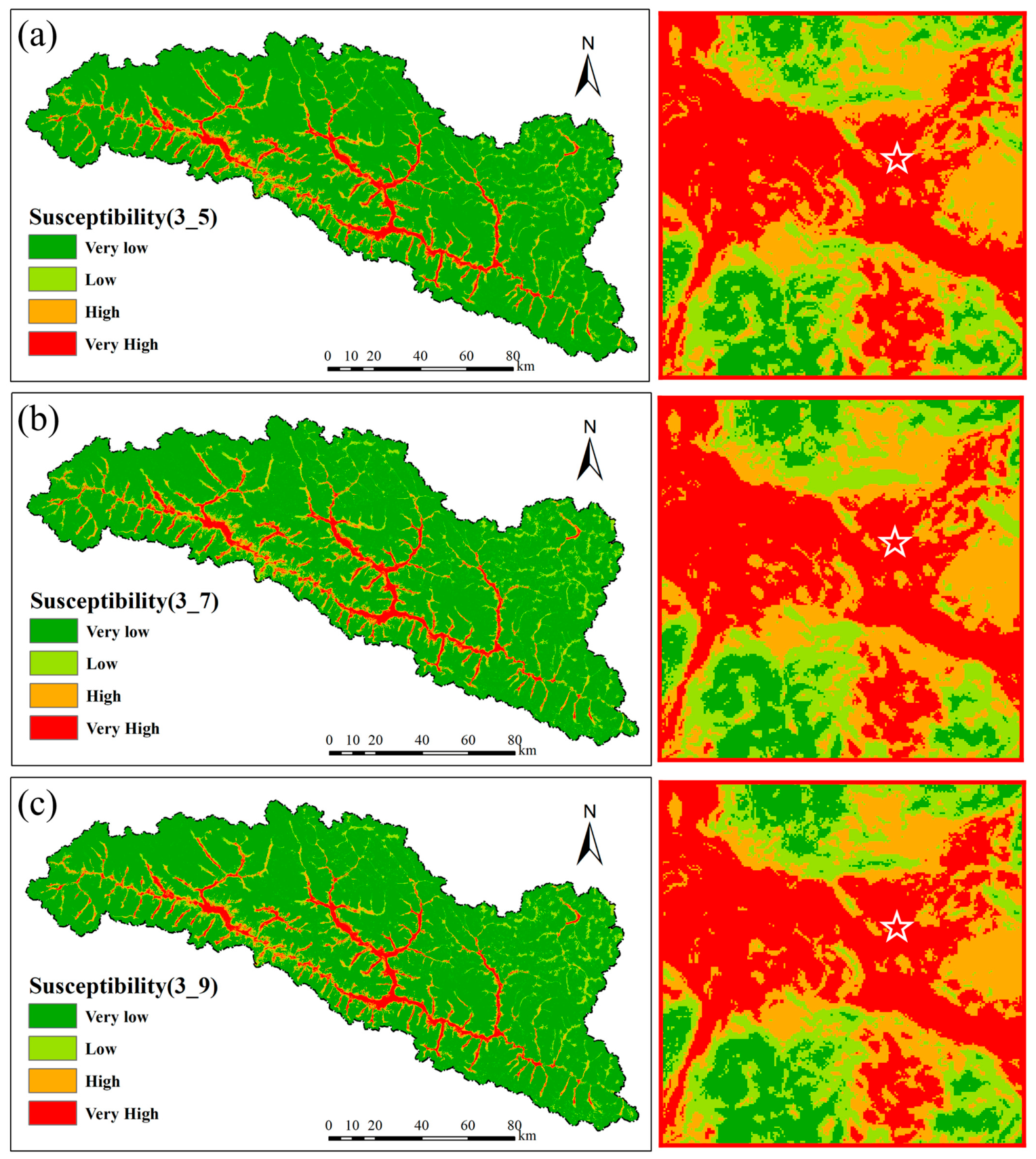
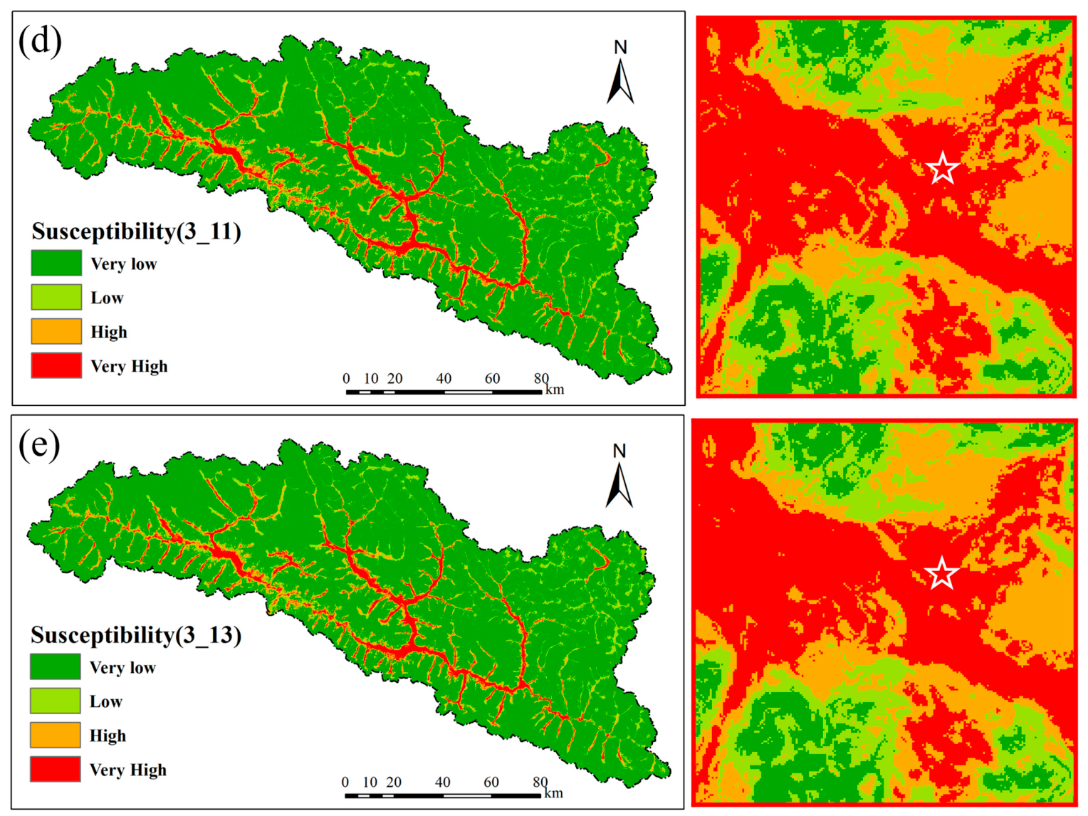
The spatial analysis extracted a high resolution subset to clarify the physical consequences of spatial scaling on sediment connectivity and to visualize the mathematical convergence detailed earlier. Figure 11 presents a 200 by 200 pixel subregion representing a physical area of six by six kilometers. This area captures the exact geographic position of a recorded major debris flow. Charting the cartographic evolution of this hazard hotspot through successive statistical windows of 5 by 5, 7 by 7, and 13 by 13 pixels, while maintaining a constant 3 by 3 construction window, illustrates the spatial enhancement process.
Operating at the most restrictive spatial scale, the susceptibility model functions as an isolated topographic detector, as the top row of Figure 11 illustrates. The resulting image exhibits extensive granular fragmentation. Because the small statistical window responds strongly to local high frequency topographic noise, the algorithm generates false positive hazard pixels across morphologically stable planar regions. Concurrently, this restricted scale fragments the continuous initiation corridor of the debris flow. The algorithm omits the broader geomorphological context, disrupting the physical continuity of sediment routing.
As the statistical window expands toward 13 by 13 pixels in the subsequent rows, the spatial limits of the susceptibility areas align with the physical boundaries of the landforms. Isolated hazard regions merge into a coherent structural hazard corridor encompassing the high risk area of the debris flow. The larger windows attenuate systematic noise in the adjacent stable ground. This visual progression supports the quantitative measures developed in this research. Increasing the neighborhood size of focal statistics enables the RF algorithm to capture sediment connectivity. The spatial configuration demonstrates that a large debris flow requires a continuous spatial connection of steep source slopes and hydrodynamic valley channels, rather than discrete high gradient pixels.
Figure 12 isolates the influence of the construction window on geomorphological representation. In this cartographic series, the methodology anchors the statistical basis at the previously identified regional scale utilizing a 13 by 13 pixel window. The localized construction matrix gradually expands to the optimal 11 by 11 pixels. To facilitate direct spatial comparison, the analysis examines a high resolution subset of 200 by 200 pixels containing the major historical debris flow.
Operating at restricted construction scales, such as 3 by 3 or 5 by 5 pixel matrices, renders the extraction of baseline topographic indicators like the TPI and surface roughness susceptible to high frequency surface artifacts within the DEMs. Despite the smoothing influence of the large 13 by 13 secondary statistical window, the underlying localized geomorphological inputs remain physically irregular. This sensitivity manifests visually as faint boundary outlines and minor false positive artifacts along morphologically stable gorge sides.
Expanding the construction window toward the optimal 11 by 11 configuration attenuates these localized topographic artifacts. The 11 by 11 matrix corresponds to a physical length of 330 m, matching the natural geometric scale of entire slope units within the incised landscape of Bomi County. Consequently, the optimal spatial configuration yields a structurally coherent susceptibility zonation map. The macroscopic landform convergence captures the major debris flow source areas and runout zones without introducing the geometric noise characteristic of isolated pixel land extraction methods.

5. Discussion

5.1. Superiority of Spatial Enhancement: Comparison with Baseline and Alternative Models

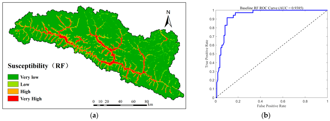
To rigorously evaluate the predictive superiority of the proposed methodology, this section presents a systematic comparative analysis between the spatially enhanced architecture and conventional benchmark algorithms. The comparative framework assesses both the cartographic rationality of the predicted hazard zones and the statistical robustness of the classification models. The primary results of this comprehensive evaluation are visually and quantitatively summarized in Figure 13.
Figure 13a illustrates the spatial distribution of debris flow susceptibility generated by the proposed spatially enhanced RF model. The map reveals that high and very high susceptibility zones concentrate along primary drainage networks and steep valley incisions, corresponding to the rugged topographic features of the study area. To quantify the physical value added by the localized geomorphological framework, the methodology incorporated an ablation study constructing a baseline isolated pixel version designated as the Traditional RF model [62]. This baseline configuration explicitly omits the neighborhood assembly indicators and relies solely on conventional macroscopic topographical features. The evaluation metrics indicate a clear performance disparity: the Traditional RF model achieves a baseline Area Under the Curve of 0.9385, whereas the proposed spatially enhanced architecture attains an improved value of 0.9434 (Figure 13b). The analysis validated this performance divergence across 20 independent model iterations to rule out random sampling biases.
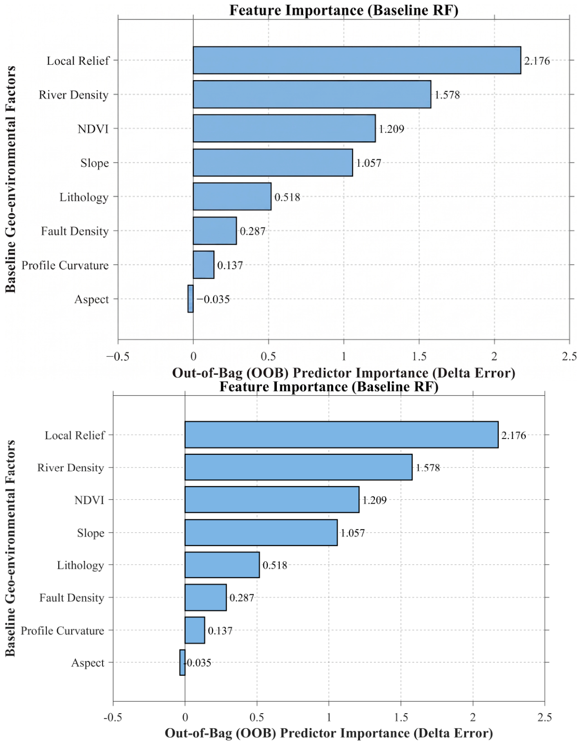
Figure 14 illustrates the internal mechanics of the baseline model via the Out of Bag feature importance. This traditional model relies heavily on individual variables, notably Local Relief scoring 2.176, River Density scoring 1.578, and the Normalized Difference Vegetation Index scoring 1.209. Although these attributes describe basic ecological conditions, relying solely on independent pixels at a macroscopic scale creates an information bottleneck. The traditional paradigm omits the continuous sediment connectivity and hydrodynamic forces linking steep source slopes and conduit valleys. Introducing the localized spatial operators resolves the assumption of pixel independence, bridging the gap between localized terrain geometry and macroscopic mass wasting kinematics [65].
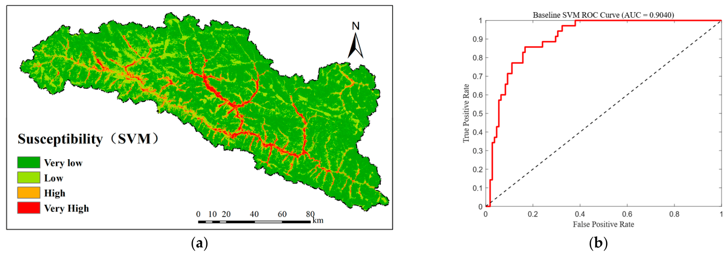
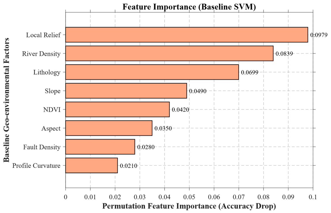
To validate the algorithmic selection, the methodology evaluated the proposed architecture against a Support Vector Machine benchmark, recognizing its structural risk minimization principles [66]. The comparison demonstrates that the benchmark records a lower predictive accuracy with an Area Under the Curve of 0.9040 (Figure 15). Analyzing the permutation feature importance of this benchmark (Figure 16) reveals that while it identifies Local Relief and River Density as dominant drivers, it fails to structurally balance the contributions of the remaining factors, exhibiting a skewed sensitivity distribution [67]. This performance constraint stems from limitations in processing geological environmental feature spaces of high dimensionality containing nonlinear and multicollinear variables. Conversely, the ensemble bagging mechanism and feature selection capabilities of the RF algorithm successfully capture the spatial heterogeneity of alpine debris flows [68].
While recent susceptibility mapping literature frequently favors hybrid modular intelligence and deep fusion networks, these data driven models encounter black box limitations and computational redundancy. Although such hybrid algorithms yield statistical improvements, they obscure physical mechanics. The spatial enhancement framework proposed in this study avoids algorithm stacking. Integrating the RF ensemble technique with physical neighborhood operators across multiple scales achieves superior predictive accuracy and preserves geomorphological interpretability. This structural transparency renders the evaluation outcomes highly operational for disaster mitigation.
The sensitivity analysis results illustrated in the associated figures validate the structural logic of the proposed modeling framework. By utilizing the structured weight database, the model dynamically filters environmental inputs, which aligns with modern novel feature selection approaches based on sensitivity metrics [52]. While traditional assessments often rely on static variable inputs, the dynamic utilization of sensitivity weights demonstrated here ensures that the ensemble architecture remains highly responsive to local data quality variations. This methodological rigor echoes the principles found in advanced neural network sensitivity evaluations [69], confirming that the identified primary driving factors physically correspond to the geomorphological realities of the study area rather than computational artifacts.

5.2. Modifiable Areal Unit Problem and Scale Sensitivity

The spatial framework encounters the Modifiable Areal Unit Problem (MAUP), where variations in the analytical unit scale directly influence predictive outcomes [70]. To validate the structural configurations, the analysis evaluated model sensitivity across a gradient of moving window sizes ranging from 3 by 3 to 15 by 15 pixels. A nonlinear relationship emerges between window size and model efficacy. Small neighborhood scales, such as the 3 by 3 and 7 by 7 matrices, respond strongly to localized topographic noise and omit the macroscopic hydrodynamic connectivity driving debris flow initiation. Conversely, spatial matrices of 15 by 15 pixels and larger introduce homogenization, diluting localized geomorphological boundaries such as steep slope incisions and channel heads. The evaluation demonstrates that intermediate configurations, specifically the 11 by 11 and 13 by 13 scales, maximize predictive capacity by balancing continuous sediment transport mechanics with the preservation of localized topographic signatures characteristic of the alpine terrain.
While spatial analysis across multiple scales introduces computational overhead compared to traditional isolated pixel models, this operational requirement remains manageable. Executing spatial operators across high resolution regional grids increases matrix operations and memory allocation. However, the resulting processing speed reduction yields critical gains in geomorphological interpretability and predictive accuracy, successfully resolving the physical limitations of pixel independence. In practical applications, modern programming platforms and parallel computing architectures effectively mitigate this computational bottleneck. Distributing focal statistics calculations across multiple processors ensures operational viability and efficient regional feature extraction across broad spatial extents.

5.3. International Context and Methodological Applicability

Contextualizing these findings within international susceptibility mapping research validates the proposed methodology. While recent studies in similar complex alpine environments utilizing conventional isolated pixel architectures report Area Under the Curve (AUC) values ranging between 0.80 and 0.88 [71], the proposed spatially enhanced framework achieves a superior predictive performance with an AUC of 0.9434 and an overall accuracy of 90.21%. This performance improvement stems directly from mitigating spatial independence assumptions. By parameterizing the spatial adjacency and sediment connectivity of macroscopic landforms, the model maintains physical consistency with actual debris flow routing mechanisms. Furthermore, the optimal 11 × 11 and 13 × 13 neighborhood scales identified in Bomi County advance previous spatial enrichment studies in the Tibetan Plateau margin, which often employed localized 3 × 3 or 5 × 5 matrices without systematic scale evaluation. These intermediate scales successfully balance localized morphological friction with macroscopic hydrodynamic convergence.
Unlike complex hybrid models (e.g., deep stacked neural networks or multi-stage ensemble hybrids) that often act as black-box predictors with excessive computational demands, the proposed multi-scale spatial operator framework explicitly encodes spatial neighborhood mechanics directly into the conditioning feature space. This approach preserves clear geomorphological interpretability, mitigates spatial overfitting caused by inventory sparsity, and achieves superior predictive performance without the parameter redundancy associated with deep hybrid architectures. Furthermore, empirical benchmarking against state-of-the-art gradient boosting algorithms—such as XGBoost (AUC = 0.9120) and LightGBM (AUC = 0.9150). Table 3 confirms that while advanced non-linear classifiers improve classification limits over standard baselines, our multi-scale spatial enrichment achieves higher predictive accuracy. This demonstrates that parameterizing spatial auto-correlation and landform continuity yields greater performance gains than merely upgrading classification algorithms on isolated pixel rasters.
Regarding geographical applicability, the methodology of spatial enrichment and landform assembly across multiple scales transfers readily to other regions. However, the optimal spatial operators identified here correspond specifically to the incised alpine terrain of Bomi County and the 30-m resolution dataset. Replicating this framework in environments possessing broader geomorphological relief or distinct hydrological catchment scales requires adjusting these threshold sizes. Future applications should conduct a preliminary scale sensitivity analysis, progressively expanding moving windows from 3 × 3 to 21 × 21 pixels, to recalibrate spatial filters according to local hydrodynamic convergence lengths. Adjusting these scale thresholds adapts this mathematical modeling strategy for various gravity-driven mass wasting environments globally.

5.4. Methodological Limitations and Future Research Directions

Utilizing a 30 m digital elevation model inherently averages localized topographic aberrations. Future research must incorporate point clouds with resolutions below one meter acquired via Light Detection and Ranging to derive precise sediment routing pathways, utilizing multiple sensor image fusion techniques to eliminate scaling noise during raster integration [72]. Furthermore, current regional mapping relies heavily on surface topography, omitting comprehensive three dimensional subsurface geomaterial characterization. The internal mechanisms of alpine mass wasting depend significantly on subsurface topography and the spatial distribution of fine grained sensitive soils. However, acquiring high density in situ geotechnical data, such as Cone Penetration Test profiles [73], remains unfeasible across Bomi County due to extreme data sparsity. Future frameworks must transition from two dimensional surface evaluations to three dimensional geological models, utilizing automated deep learning algorithms to predict subsurface structural heterogeneity [47].
The current methodology performs a static spatial susceptibility assessment [49], restricted by the absence of precise historical timestamps for documented events. This static approach introduces temporal survivorship bias and omits transient hydrometeorological triggering forces. Overcoming this temporal nonstationarity requires integrating continuous meteorological rainfall sequences and Small Baseline Subset Interferometric Synthetic Aperture Radar to quantify the transient accumulation of loose solid material. Moreover, the existing data driven framework omits the physical laws governing debris flow kinematics. Future methodologies should transition toward dual driven physics and data models. Exploring Physics Informed Neural Networks allows for the direct incorporation of geomechanical laws into deep learning loss functions, transforming susceptibility mapping from a spatial classification problem into a mechanics based early warning tool [74].
While the current spatial framework demonstrates high accuracy in identifying static susceptibility zones, fully capturing physical kinematics requires addressing temporal predictive capabilities under changing environmental conditions. Future operational deployments will necessitate a continuous updating procedure and dynamic filtering mechanisms to calibrate the susceptibility boundaries for sequential upcoming events [75]. Furthermore, the robustness of the predictive model to environmental noise, missing data, or remote sensing sensor malfunction is a critical consideration. Although the inherent bagging mechanism of the Random Forest architecture naturally resists minor data corruption, implementing automated data normalization and dynamic temporal filtering will be essential to sustain model reliability during extreme climatic fluctuations.
Finally, the historical debris flow inventory relies on documented field surveys, introducing potential spatial bias if observations favor accessible infrastructural corridors over remote catchments. Although the spatially constrained negative sampling strategy mitigates background bias during training, epistemic uncertainties impact the final predictive distribution [76]. The multiple scale spatial operators and the trained ensemble structure were explicitly calibrated to the extreme topographic incision and specific monsoonal climate of the Tibetan Plateau. Applying this configuration to regions with different hydro climatic baselines requires extensive structural recalibration. Furthermore, while the physical principles embedded within the multi-scale geo-environmental variables suggest strong theoretical transferability to other steep mountainous catchments, direct empirical cross-regional external validation remains an essential next step. Consequently, executing cross regional evaluations utilizing independent external datasets remains a critical objective to test the geographic adaptability of these localized geomorphological indicators across diverse mass wasting environments globally.

6. Conclusions

This study proposed a spatially enhanced RF framework based on multi-scale micro-geomorphic parameters to evaluate debris flow susceptibility in the extreme alpine terrain of Bomi County. By systematically contrasting this framework against pixel-isolated baselines, the following data-justified conclusions are drawn:
(1)
Predictive Superiority of Spatial Enhancement: The integration of spatial neighborhood operators significantly enhances the predictive robustness of the RF algorithm. The proposed spatially enhanced model achieved an outstanding AUC of 0.9434, substantially outperforming the pixel-isolated Traditional-RF baseline and the standard SVM benchmark. This quantitatively proves that resolving the pixel-independence misconception is critical for accurate regional hazard mapping.
(2)
Optimal Scale for Micro-Geomorphic Connectivity: The analytical results demonstrate a distinct scale-dependent effect in topographic feature extraction. Spatial moving windows of 11 × 11 and 13 × 13 pixels were identified as the optimal analytical scales. These specific configurations effectively filter high-frequency localized noise while preserving the structural boundaries of critical mass-wasting conduits, thereby successfully capturing the macro-scale hydrodynamic connectivity of debris flows.
(3)
Dominance of Topographic Mechanisms: The rigorous MDG sensitivity analysis confirms that debris flow susceptibility in Bomi County is primarily dictated by multi-scale topographic variance rather than static land-cover or absolute geological classifications. Micro-geomorphic indicators, particularly those reflecting local relief and slope configuration within the optimal spatial windows, exhibit the highest predictive weights, underscoring the necessity of high-resolution topographic parameterization.
(4)
Operational Boundaries and Future Outlook: While the framework demonstrates excellent spatial calibration for the highly incised Tibetan Plateau environment, it fundamentally represents a static, site-specific evaluation. Its immediate generalizability is strictly bounded by the specific hydro-climatic and lithological baseline of the study area. Future investigations must incorporate independent external datasets, automated 3D subsurface geo-models, and time-series environmental data to achieve cross-regional validation and dynamic spatio-temporal forecasting.

Author Contributions

J.C. contributed to investigation, data curation, methodology, writing—original draft. G.X. contributed to writing—review & editing, Funding acquisition. All authors have read and agreed to the published version of the manuscript.

Funding

This research was funded by the China Geological Survey Applied Geological Survey Project, grant number DD20242171.

Institutional Review Board Statement

Not applicable.

Informed Consent Statement

Not applicable.

Data Availability Statement

The raw data supporting the conclusions of this article will be made available by the authors on request.

Conflicts of Interest

The authors declare no conflicts of interest.

Appendix A

Figure A1. Debris flow susceptibility map based on the combination of a 3 × 3 neighborhood statistical window and a 5 × 5 localized geomorphological construction window.
Applsci 16 08585 g0a1
Figure A2. Debris flow susceptibility map based on the combination of a 3 × 3 neighborhood statistical window and a 7 × 7 localized geomorphological construction window.
Applsci 16 08585 g0a2
Figure A3. Debris flow susceptibility map based on the combination of a 3 × 3 neighborhood statistical window and a 9 × 9 localized geomorphological construction window.
Applsci 16 08585 g0a3
Figure A4. Debris flow susceptibility map based on the combination of a 3 × 3 neighborhood statistical window and a 11 × 11 localized geomorphological construction window.
Applsci 16 08585 g0a4
Figure A5. Debris flow susceptibility map based on the combination of a 3 × 3 neighborhood statistical window and a 13 × 13 localized geomorphological construction window.
Applsci 16 08585 g0a5
Figure A6. Debris flow susceptibility map based on the combination of a 5 × 5 neighborhood statistical window and a 5 × 5 localized geomorphological construction window.
Applsci 16 08585 g0a6
Figure A7. Debris flow susceptibility map based on the combination of a 5 × 5 neighborhood statistical window and a 7 × 7 localized geomorphological construction window.
Applsci 16 08585 g0a7
Figure A8. Debris flow susceptibility map based on the combination of a 5 × 5 neighborhood statistical window and a 9 × 9 localized geomorphological construction window.
Applsci 16 08585 g0a8
Figure A9. Debris flow susceptibility map based on the combination of a 5 × 5 neighborhood statistical window and a 11 × 11 localized geomorphological construction window.
Applsci 16 08585 g0a9
Figure A10. Debris flow susceptibility map based on the combination of a 5 × 5 neighborhood statistical window and a 13 × 13 localized geomorphological construction window.
Applsci 16 08585 g0a10
Figure A11. Debris flow susceptibility map based on the combination of a 7 × 7 neighborhood statistical window and a 5 × 5 localized geomorphological construction window.
Applsci 16 08585 g0a11
Figure A12. Debris flow susceptibility map based on the combination of a 7 × 7 neighborhood statistical window and a 7 × 7 localized geomorphological construction window.
Applsci 16 08585 g0a12
Figure A13. Debris flow susceptibility map based on the combination of a 7 × 7 neighborhood statistical window and a 9 × 9 localized geomorphological construction window.
Applsci 16 08585 g0a13
Figure A14. Debris flow susceptibility map based on the combination of a 7 × 7 neighborhood statistical window and a 11 × 11 localized geomorphological construction window.
Applsci 16 08585 g0a14
Figure A15. Debris flow susceptibility map based on the combination of a 7 × 7 neighborhood statistical window and a 13 × 13 localized geomorphological construction window.
Applsci 16 08585 g0a15
Figure A16. Debris flow susceptibility map based on the combination of a 9 × 9 neighborhood statistical window and a 5 × 5 localized geomorphological construction window.
Applsci 16 08585 g0a16
Figure A17. Debris flow susceptibility map based on the combination of a 9 × 9 neighborhood statistical window and a 7 × 7 localized geomorphological construction window.
Applsci 16 08585 g0a17
Figure A18. Debris flow susceptibility map based on the combination of a 9 × 9 neighborhood statistical window and a 9 × 9 localized geomorphological construction window.
Applsci 16 08585 g0a18
Figure A19. Debris flow susceptibility map based on the combination of a 9 × 9 neighborhood statistical window and a 11 × 11 localized geomorphological construction window.
Applsci 16 08585 g0a19
Figure A20. Debris flow susceptibility map based on the combination of a 9 × 9 neighborhood statistical window and a 13 × 13 localized geomorphological construction window.
Applsci 16 08585 g0a20
Figure A21. Debris flow susceptibility map based on the combination of a 11 × 11 neighborhood statistical window and a 5 × 5 localized geomorphological construction window.
Applsci 16 08585 g0a21
Figure A22. Debris flow susceptibility map based on the combination of a 11 × 11 neighborhood statistical window and a 7 × 7 localized geomorphological construction window.
Applsci 16 08585 g0a22
Figure A23. Debris flow susceptibility map based on the combination of a 11 × 11 neighborhood statistical window and a 9 × 9 localized geomorphological construction window.
Applsci 16 08585 g0a23
Figure A24. Debris flow susceptibility map based on the combination of a 11 × 11 neighborhood statistical window and a 11 × 11 localized geomorphological construction window.
Applsci 16 08585 g0a24
Figure A25. Debris flow susceptibility map based on the combination of a 11 × 11 neighborhood statistical window and a 13 × 13 localized geomorphological construction window.
Applsci 16 08585 g0a25

References

  1. Wei, L.; Zhang, X.; Zhang, H.; Xu, Y.; Ao, M.; Dai, Y.; Tolomei, C.; Liu, S.; Dong, F.; Li, B.; et al. Debris flow risk assessment via numerical simulation: A case study in Northeast China. Landslides 2025, 22, 3429–3454. [Google Scholar] [CrossRef] [Scilit]
  2. Liu, S.; Liu, S.; Lv, D.; Wei, L.; Ao, M.; Pan, X.; Li, B.; Cui, Y.; Wang, L.; He, X. Debris flow susceptibility and hazard assessment in Fushun based on hydrological response units. Nat. Hazards 2024, 120, 8667–8693. [Google Scholar] [CrossRef] [Scilit]
  3. Shah, N.A.; Shafique, M.; Owen, L.A.; Al-Mulla, Y.; Ullah, Y. Morphometric analysis of debris flow hazard and risk assessment in the mountain terrains of northern Pakistan using remote sensing and field data. Earth Sci. Inform. 2025, 18, 295. [Google Scholar] [CrossRef] [Scilit]
  4. Urs, M.S.; Nagendra, P.; Vinay, C.; Kumar, B.S.; Narasimha, K.P. Morpho-tectonic analysis of an upstream sub-basin of the Cauvery River from Bhagamandala to Shivanasamudra using geomorphic indices using GIS. J. Geomat. 2025, 19, 165–174. [Google Scholar] [CrossRef] [Scilit]
  5. Dallons Thanneur, L.; Giacona, F.; Eckert, N.; Frey, P. Constitution of a multicentennial multirisk database in a mountainous environment from composite sources: The example of the Vallouise-Pelvoux municipality (Ecrins, France). Nat. Hazards Earth Syst. Sci. 2025, 25, 4881–4906. [Google Scholar] [CrossRef] [Scilit]
  6. Peleg, N.; Koukoula, M.; Marra, F. A 2 °C warming can double the frequency of extreme summer downpours in the Alps. npj Clim. Atmos. Sci. 2025, 8, 216. [Google Scholar] [CrossRef] [Scilit]
  7. Rashid, M.A.; Leonelli, G.; Chelli, A. Quantitative characterization of geomorphological and topographical features of debris-flow channels at the Alpe di Succiso mountain, Northern Apennines (Italy). J. Maps 2024, 20, 2422549. [Google Scholar] [CrossRef] [Scilit]
  8. Dinh, N.C.; Manh, N.D.; Lan, N.C.; Tuan, N.A.; Prakash, I.; Dung, V.Q.; Van Thang, N. GIS-based Flow-R model for debris flow susceptibility mapping: A case study from Muong Bo, Lao Cai, Vietnam. J. Sci. Transp. Technol. 2026, 6, 29–47. [Google Scholar] [CrossRef] [Scilit]
  9. Niyogakiza, A.; Liu, Q. GIS-driven multi-criteria assessment of rural settlement patterns and attributes in Rwanda’s Western Highlands (Central Africa). Sustainability 2025, 17, 6406. [Google Scholar] [CrossRef] [Scilit]
  10. Li, J.; Adhikari, B.R.; Ding, X.; Wu, S.; Meng, X.; Niu, Z.; Pei, X.; Zhan, Y.; Di, B. Frequent dry-wet cycles promote debris flow occurrence: Insights from 40 years of data in subtropical monsoon region of Sichuan, China. Catena 2024, 238, 107888. [Google Scholar] [CrossRef] [Scilit]
  11. Wei, L.; Xu, Y.; Lv, D.; Cui, H.; Liu, S.; Ao, M. Rockfall susceptibility assessment in Kuandian County (Northeast China) by combining information content method and analytic hierarchy process. Bull. Eng. Geol. Environ. 2024, 83, 240. [Google Scholar] [CrossRef] [Scilit]
  12. Ming, Z.; Zhang, J.; He, H.; Zhang, L.; Chen, R.; Jia, Y. Addressing accuracy challenges in machine learning for debris flow susceptibility: Insights from the Yalong River basin. J. Mt. Sci. 2025, 22, 2034–2052. [Google Scholar] [CrossRef] [Scilit]
  13. Liu, Y.; Chen, J.; Sun, X.; Li, Y.; Zhang, Y.; Xu, W.; Yan, J.; Ji, Y.; Wang, Q. A progressive framework combining unsupervised and optimized supervised learning for debris flow susceptibility assessment. Catena 2024, 234, 107560. [Google Scholar] [CrossRef] [Scilit]
  14. Jiang, N.; Su, F.; Wei, R.; Huang, Y.; Jin, W.; Huang, P.; Zeng, Q. Dependence of debris flow susceptibility maps on sampling strategy with data-driven grid-based model. Ecol. Indic. 2024, 166, 112534. [Google Scholar] [CrossRef] [Scilit]
  15. Mehmood, Q.; Tekin, S.; Çan, T. A hybrid approach to earthquake-preconditioned debris flow: Regional susceptibility and event-based hazard assessments. Nat. Hazards 2026, 122, 440. [Google Scholar] [CrossRef] [Scilit]
  16. Ullah, H.; Wang, W.; Daud, H.; Hussain, M.A.; Ali, N. Integrating machine learning and deep learning for enhanced landslide susceptibility and propagation dynamics in Northwestern Pakistan. Bull. Eng. Geol. Environ. 2026, 85, 254. [Google Scholar] [CrossRef] [Scilit]
  17. Jaman, T.; Bhaskar, S.; Swain, S.K.; Alam, S. A hybrid geospatial framework for flood hazard zonation using AHP and machine learning: Case study of Kaziranga Tiger Reserve, India. Glob. Earth Surf. Process. Change 2026, 7, 100021. [Google Scholar] [CrossRef] [Scilit]
  18. Chen, H.; Ma, T.; Shen, L.; Ye, B.; Ni, S.; Ni, X.; Sun, H. Negative sample selection for landslide susceptibility prediction: A hybrid optimization approach using an AHP-KDE multi-ring sampling strategy. Ecol. Indic. 2025, 180, 114304. [Google Scholar] [CrossRef] [Scilit]
  19. Kumar, A.; Sarkar, R. Debris flow susceptibility evaluation—A review. Iran. J. Sci. Technol. Trans. Civ. Eng. 2023, 47, 1277–1292. [Google Scholar] [CrossRef] [Scilit]
  20. Daud, H.; Dou, J.; Tanoli, J.I.; Ali, N.; Khan, N.G.; Xiang, Z.; Dong, A.; Xing, K.; Ullah, H.; Zhang, L. The role of multi-resolution DEMs and sampling strategy uncertainty in deep learning-based debris flow susceptibility mapping. Acta Geotech. 2026, 21, 395–418. [Google Scholar] [CrossRef] [Scilit]
  21. Luo, J.; Zheng, Z.; Li, T.; He, S.; Tarolli, P. Impact of tillage-induced microtopography on hydrological-sediment connectivity and its hydrodynamic understanding. Catena 2023, 228, 107168. [Google Scholar] [CrossRef] [Scilit]
  22. Torresani, L.; Piton, G.; D’Agostino, V. Morphodynamics and sediment connectivity index in an unmanaged, debris-flow prone catchment: A through time perspective. J. Mt. Sci. 2023, 20, 891–910. [Google Scholar] [CrossRef] [Scilit]
  23. Rahmati, O.; Soleimanpour, S.M.; Arabkhedri, M.; Mehrjo, S.; Kalantari, Z.; Cavalli, M.; Crema, S.; Bahmani, A. Towards quantification of soil conservation performance using sediment connectivity concept at hillslope scale: Proposing a new framework for data-scarce regions. J. Soils Sediments 2023, 23, 2298–2309. [Google Scholar] [CrossRef] [Scilit]
  24. Wu, W.; Zhang, M.; Chen, C.; Chen, Z.; Yang, H.; Su, H. Coastal reclamation shaped narrower and steeper tidal flats in Fujian, China: Evidence from time-series satellite data. Ocean Coast. Manag. 2024, 247, 106933. [Google Scholar] [CrossRef] [Scilit]
  25. Zhang, H.; Zhang, D.; Zhou, Y.; Cutler, M.E.; Cui, D.; Zhang, Z. Quantitative analysis of the interaction between wind turbines and topography change in intertidal wind farms by remote sensing. J. Mar. Sci. Eng. 2022, 10, 504. [Google Scholar] [CrossRef] [Scilit]
  26. Bernard, M.; Barbini, M.; Berti, M.; Boreggio, M.; Simoni, A.; Gregoretti, C. Rainfall-runoff modeling in rocky headwater catchments for the prediction of debris flow occurrence. Water Resour. Res. 2025, 61, e2023WR036887. [Google Scholar] [CrossRef] [Scilit]
  27. Wang, H.; Liu, R.; Song, Y.; Wang, Y.; Cai, C.; Wang, J. Modeling to evaluate permanent gully susceptibility and dominant controlling factors analysis in the black soil region of Northeast China. Soil Tillage Res. 2025, 252, 106595. [Google Scholar] [CrossRef] [Scilit]
  28. Liu, W.; He, S. Influence of runoff on debris flow propagation at a catchment scale: A case study. Landslides 2024, 21, 1757–1774. [Google Scholar] [CrossRef] [Scilit]
  29. Fu, X.; Zhu, X.; Xu, Q.; Zhu, H.; Yuan, R.; Li, J. Decadal landslide susceptibility mapping: Impacts of sampling methods on prediction accuracy. J. Mt. Sci. 2025, 22, 4157–4173. [Google Scholar] [CrossRef] [Scilit]
  30. Baggio, T.; Martini, M.; Bettella, F.; D’Agostino, V. Debris flow and debris flood hazard assessment in mountain catchments. Catena 2024, 245, 108338. [Google Scholar] [CrossRef] [Scilit]
  31. Singh, S.; Raju, A.; Rosi, A.; Singh, R.; Floris, M.; Meena, S.R. Integrating geomorphology-based terrain segmentation with machine learning for landslide susceptibility assessment in the Darjeeling-Sikkim Himalaya, India. Preprint 2026. [Google Scholar] [CrossRef] [Scilit]
  32. He, S.; Chen, W.; Chen, X.; Wang, D.; Li, Y.; Pei, Z.; Zhao, P.; Qi, Y. Mechanisms and benefits of segmented eco-geotechnical measures for debris flow mitigation. Ecol. Eng. 2025, 216, 107621. [Google Scholar] [CrossRef] [Scilit]
  33. Guo, J.; Wang, Y.; Li, Y. Topographic controls on the initiation and transport of landslide-triggered debris flows. Geomorphology 2025, 486, 109901. [Google Scholar] [CrossRef] [Scilit]
  34. Lü, Q.; Yang, K.; Zhang, W.; Wang, L.; Wang, L. Machine learning-based assessment of future debris flow susceptibility under CMIP6 precipitation scenarios in Qinghai Province, China. Geoenviron. Disasters 2026, 13, 40. [Google Scholar] [CrossRef] [Scilit]
  35. Li, A.; Gao, K.; Wei, A.; Li, H.; Wu, J.; Wang, J.; Zhang, Y. Comparison of machine learning algorithms combined with metaheuristic-based feature selection methods for debris flow susceptibility assessments. Geomat. Nat. Hazards Risk 2026, 17, 2698970. [Google Scholar] [CrossRef] [Scilit]
  36. Zhao, H.; Wei, A.; Ma, F.; Dai, F.; Jiang, Y.; Li, H. Comparison of debris flow susceptibility assessment methods: Support vector machine, particle swarm optimization, and feature selection techniques. J. Mt. Sci. 2024, 21, 397–412. [Google Scholar] [CrossRef] [Scilit]
  37. Cao, J.; Qin, S.; Yao, J.; Zhang, C.; Liu, G.; Zhao, Y.; Zhang, R. Debris flow susceptibility assessment based on information value and machine learning coupling method: From the perspective of sustainable development. Environ. Sci. Pollut. Res. 2023, 30, 87500–87516. [Google Scholar] [CrossRef] [Scilit]
  38. Qin, Z.; Peng, Q.; Jin, C.; Xu, J.; Xing, S.; Zhu, P.; Yang, G. Geographically weighted random forest fusing multi-source environmental covariates for spatial prediction of soil heavy metals. Environ. Pollut. 2025, 385, 127135. [Google Scholar] [CrossRef] [Scilit]
  39. Yu, R.; Guo, R.; Jiang, L.; Shao, Y.; Zhou, Z. Susceptibility assessment of glacier-related debris flow on the southeastern Tibetan Plateau using different hybrid machine learning models. Sci. Total Environ. 2024, 954, 176400. [Google Scholar] [CrossRef] [Scilit]
  40. Bu, J.; Liu, S.; Yang, H.; Wang, Z.; Zuo, X. Cryosphere remote sensing using multisource satellite data: Sensor technologies, current status, challenges, and opportunities. IEEE J. Sel. Top. Appl. Earth Obs. Remote Sens. 2026, 19, 20147–20204. [Google Scholar] [CrossRef] [Scilit]
  41. Chang, L.; Wu, T.; He, H.; Li, B.; Zhang, R. Glacial debris flow hazard assessment and multi-parameter probabilistic model: A case study of Guxiang Gully. Landslides 2025, 22, 2749–2768. [Google Scholar] [CrossRef] [Scilit]
  42. Zheng, J.; Zhao, Y.; Huo, F.; Li, Y.; Meng, X.; Yue, D.; Guo, F.; Zhang, Y. Quantitative assessment method for catastrophic debris flow risks in the Bailong River Basin, China. Geomat. Nat. Hazards Risk 2026, 17, 2653716. [Google Scholar] [CrossRef] [Scilit]
  43. Li, Y.; Wang, Y.; Wang, X.; Qi, J.; Zhang, X.; Lin, Q. Risk assessment of glacial debris flow on highway under warming climate: A case study of Tianmo Gully in the southeastern Tibetan Plateau. Ecol. Indic. 2024, 167, 112606. [Google Scholar] [CrossRef] [Scilit]
  44. Feng, L.; Zhang, M.; Mao, Y.; Liu, H.; Yang, C.; Dong, Y.; Nanehkaran, Y.A. Convolutional neural network-based deep learning for landslide susceptibility mapping in the Bakhtegan watershed. Sci. Rep. 2025, 15, 13250. [Google Scholar] [CrossRef] [Scilit]
  45. Krinkin, K.; Shichkina, Y. Cognitive architecture for co-evolutionary hybrid intelligence. In Proceedings of the International Conference on Artificial General Intelligence; Springer International Publishing: Cham, Switzerland, 2022; pp. 293–303. [Google Scholar] [CrossRef] [Scilit]
  46. Shahri, A.A.; Moud, F.M. Landslide susceptibility mapping using hybridized block modular intelligence model. Bull. Eng. Geol. Environ. 2021, 80, 267–284. [Google Scholar] [CrossRef] [Scilit]
  47. Shahri, A.A.; Chunling, S.; Larsson, S. A hybrid ensemble-based automated deep learning approach to generate 3D geo-models and uncertainty analysis. Eng. Comput. 2024, 40, 1501–1516. [Google Scholar] [CrossRef] [Scilit]
  48. Fu, Y.; Fan, Z.; Li, X.; Wang, P.; Sun, X.; Ren, Y.; Cao, W. The influence of non-landslide sample selection methods on landslide susceptibility prediction. Land 2025, 14, 722. [Google Scholar] [CrossRef] [Scilit]
  49. Shahri, A.A.; Spross, J.; Johansson, F.; Larsson, S. Landslide susceptibility hazard map in southwest Sweden using artificial neural network. Catena 2019, 183, 104225. [Google Scholar] [CrossRef] [Scilit]
  50. Linardatos, P.; Papastefanopoulos, V.; Kotsiantis, S. Explainable AI: A review of machine learning interpretability methods. Entropy 2020, 23, 18. [Google Scholar] [CrossRef] [Scilit]
  51. Bhattarai, T.R.; Bhandary, N.P. Comparative analysis of slope and grid units for co-seismic landslide susceptibility mapping using machine learning methods. Discov. Geosci. 2026, 4, 121. [Google Scholar] [CrossRef] [Scilit]
  52. Asheghi, R.; Hosseini, S.A.; Saneie, M.; Shahri, A.A. Updating the neural network sediment load models using different sensitivity analysis methods: A regional application. J. Hydroinform. 2020, 22, 562–577. [Google Scholar] [CrossRef] [Scilit]
  53. Zheng, J.; Du, J.; Wang, B.; Klemeš, J.J.; Liao, Q.; Liang, Y. A hybrid framework for forecasting power generation of multiple renewable energy sources. Renew. Sustain. Energy Rev. 2023, 172, 113046. [Google Scholar] [CrossRef] [Scilit]
  54. Gharoun, H.; Yazdanjue, N.; Khorshidi, M.S.; Chen, F.; Gandomi, A.H. Leveraging neural networks and calibration measures for confident feature selection. IEEE Trans. Emerg. Top. Comput. Intell. 2025, 9, 2179–2193. [Google Scholar] [CrossRef] [Scilit]
  55. Pizarroso, J.; Portela, J.; Muñoz, A. NeuralSens: Sensitivity analysis of neural networks. J. Stat. Softw. 2022, 102, 1–36. [Google Scholar] [CrossRef] [Scilit]
  56. Omomule, T.; Engelbrecht, A. Sensitivity analysis of neural network ensembles to data quality issues. In Proceedings of the 2025 International Conference on Artificial Intelligence, Computer, Data Sciences and Applications (ACDSA), Durban, South Africa, 20–22 August 2025; IEEE: Piscataway, NJ, USA, 2025; pp. 1–8. [Google Scholar] [CrossRef] [Scilit]
  57. Reid, M.E.; Ochiai, H. Dynamic evolution from shallow landslide to fluidized debris flow in a field-scale experiment. Landslides 2025, 22, 3657–3668. [Google Scholar] [CrossRef] [Scilit]
  58. Breiman, L. Random forests. Mach. Learn. 2001, 45, 5–32. [Google Scholar] [CrossRef] [Scilit]
  59. Chowdhury, M.S.; Rahman, M.N.; Sheikh, M.S.; Sayeid, M.A.; Mahmud, K.H.; Hafsa, B. GIS-based landslide susceptibility mapping using logistic regression, random forest and decision and regression tree models in Chattogram District, Bangladesh. Heliyon 2024, 10, e23424. [Google Scholar] [CrossRef] [Scilit]
  60. Huang, Z.; Gong, D.; Tang, C.; Wang, J.; Zhang, C.; Dang, K.; Chai, X.; Wang, J.; Yan, Z. A risk prediction model for neovascular glaucoma secondary to proliferative diabetic retinopathy based on Boruta feature selection and random forest. Front. Cell Dev. Biol. 2025, 13, 1604832. [Google Scholar] [CrossRef] [Scilit]
  61. Li, L.; Sun, W.; Ayti, A.; Chen, W.; Liu, Z.; Gómez-Zamorano, L.Y. Machine learning modeling of foam concrete performance: Predicting mechanical strength and thermal conductivity from material compositions. Appl. Sci. 2025, 15, 7125. [Google Scholar] [CrossRef] [Scilit]
  62. Miftahushudur, T.; Sahin, H.M.; Grieve, B.; Yin, H. A survey of methods for addressing imbalanced data problems in agriculture applications. Remote Sens. 2025, 17, 454. [Google Scholar] [CrossRef] [Scilit]
  63. Wang, Y.; Wang, L.; Liu, S.; Liu, P.; Zhu, Z.; Zhang, W. A comparative study of regional landslide susceptibility mapping with multiple machine learning models. Geol. J. 2024, 59, 2383–2400. [Google Scholar] [CrossRef] [Scilit]
  64. Tian, Y.; Zeng, T.; Wang, L.; Chen, G.; Yang, S.; Chen, H.; Wang, L. Spectral feature integration and ensemble learning optimization for regional-scale landslide susceptibility mapping in mountainous areas. Remote Sens. 2026, 18, 382. [Google Scholar] [CrossRef] [Scilit]
  65. Gui, B.; Bhardwaj, A.; Sam, L.; Sam, B.C.; Ahmed, R.; Ali, S.N.; Pandey, P.; Vatsal, S.; Martin-Torres, J. Scalable landslide detection in complex Himalayan topography via a novel object-based residual graph attention network. Geosci. Front. 2026, 17, 102401. [Google Scholar] [CrossRef] [Scilit]
  66. Liu, D.; Zhou, J.; Sang, X.; Tang, D.; Zhang, S.; Chen, Q. Machine learning-based identification of potential debris flow catchments in the Wenchuan earthquake region. Earth Sci. Inform. 2025, 18, 515. [Google Scholar] [CrossRef] [Scilit]
  67. Abdelaziz, M.T.; Radwan, A.; Mamdouh, H.; Saad, A.S.; Abuzaid, A.S.; AbdElhakeem, A.A.; Zakzouk, S.; Moussa, K.; Darweesh, M.S. Enhancing network threat detection with random forest-based NIDS and permutation feature importance. J. Netw. Syst. Manag. 2025, 33, 2. [Google Scholar] [CrossRef] [Scilit]
  68. Kaynak, T. A systematic framework for the integration of feature selection and artificial intelligence in landslide susceptibility assessment. Nat. Hazards 2026, 122, 91. [Google Scholar] [CrossRef] [Scilit]
  69. Xu, A.; Wang, R.; Weng, X.; Wu, Q.; Zhuang, L. Strategic integration of adaptive sampling and ensemble techniques in federated learning for aircraft engine remaining useful life prediction. Appl. Soft Comput. 2025, 175, 113067. [Google Scholar] [CrossRef] [Scilit]
  70. Erener, A.; Düzgün, H.S.B. Landslide susceptibility assessment: What are the effects of mapping unit and mapping method? Environ. Earth Sci. 2012, 66, 859–877. [Google Scholar] [CrossRef] [Scilit]
  71. Li, Y.; Jiang, W.; Feng, X.; Lv, S.; Yu, W.; Ma, E. Debris flow susceptibility mapping in alpine canyon region: A case study of Nujiang Prefecture. Bull. Eng. Geol. Environ. 2024, 83, 169. [Google Scholar] [CrossRef] [Scilit]
  72. Mishra, V.K.; Nareti, U.; Kumar, R.; Pant, T.; Aleem, A.; Singh, A.; Biable, S.E. GDF: A novel image fusion approach for compelling depiction of earthly features. J. Sens. 2023, 2023, 9429505. [Google Scholar] [CrossRef] [Scilit]
  73. Ghaderi, A.; Shahri, A.A.; Larsson, S. An artificial neural network based model to predict spatial soil type distribution using piezocone penetration test data (CPTu). Bull. Eng. Geol. Environ. 2019, 78, 4579–4588. [Google Scholar] [CrossRef] [Scilit]
  74. Cui, H.; Pei, T.; Devineni, N.; Tian, Y.; Shen, C.; Ji, J. A multi-objective physics-informed machine learning framework for landslide susceptibility mapping. Georisk Asses. Manag. Risk Eng. Syst. Geohazards 2026, 20, 1–25. [Google Scholar] [CrossRef] [Scilit]
  75. Cai, J.; Liu, G.; Jia, H.; Zhang, B.; Wu, R.; Fu, Y.; Yu, J.; Zhang, R. A new algorithm for landslide dynamic monitoring with high temporal resolution by Kalman filter integration of multiplatform time-series InSAR processing. Int. J. Appl. Earth Obs. Geoinf. 2022, 110, 102812. [Google Scholar] [CrossRef] [Scilit]
  76. Shahri, A.A.; Chunling, S.; Larsson, S. A novel approach to uncertainty quantification in groundwater table modeling by automated predictive deep learning. Nat. Resour. Res. 2022, 31, 1351–1373. [Google Scholar] [CrossRef] [Scilit]
Figure 1. Location, digital elevation, and historical debris flow distribution of the Parlung Tsangpo River Basin. (Left) Regional location and drainage network within the Xizang Autonomous Region. (Right) DEM layer showing primary watercourses, highway networks, and magnitude-classified debris flow events.
Applsci 16 08585 g001
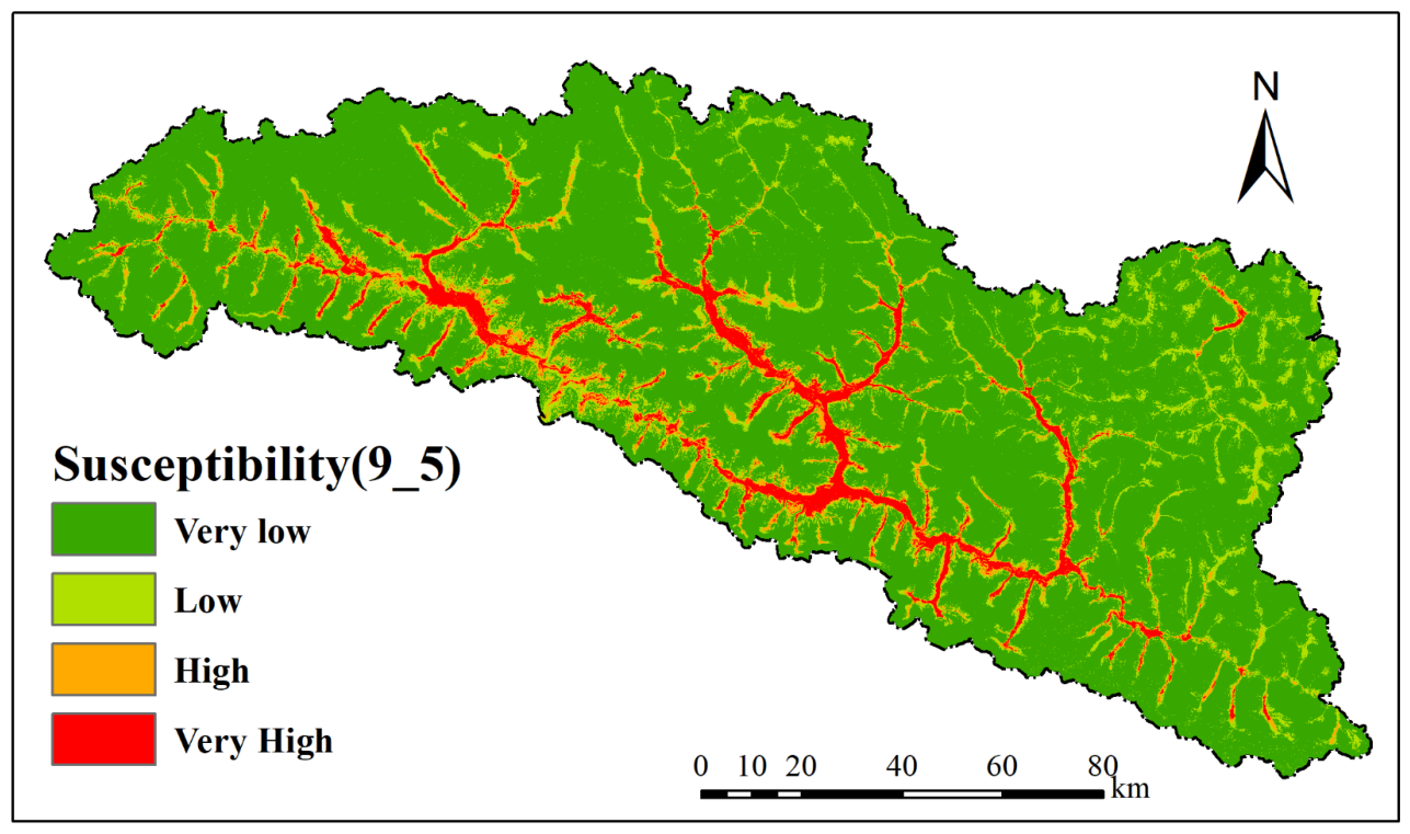
Figure 2. Topographic Indicators. (a) Slope. (b) Aspect. (c) Elevation difference. (d) Profile curvature.
Applsci 16 08585 g002
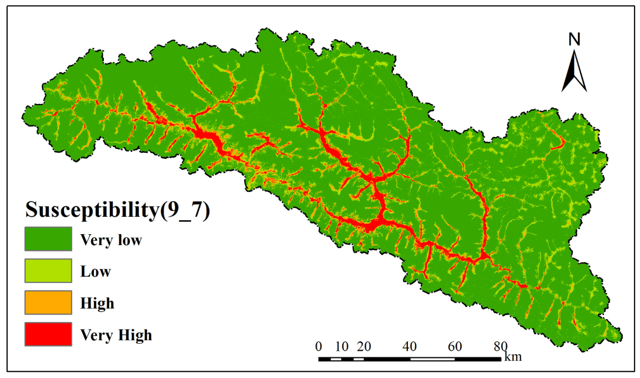
Figure 3. Micro-geomorphic Indicators. (a) Slope (3 × 3). (b) TPI (3 × 3). (c) Roughness. (d) Total Curvature (3 × 3). (e) Profile Curvature (3 × 3) (f) Local Relief (3 × 3).
Applsci 16 08585 g003
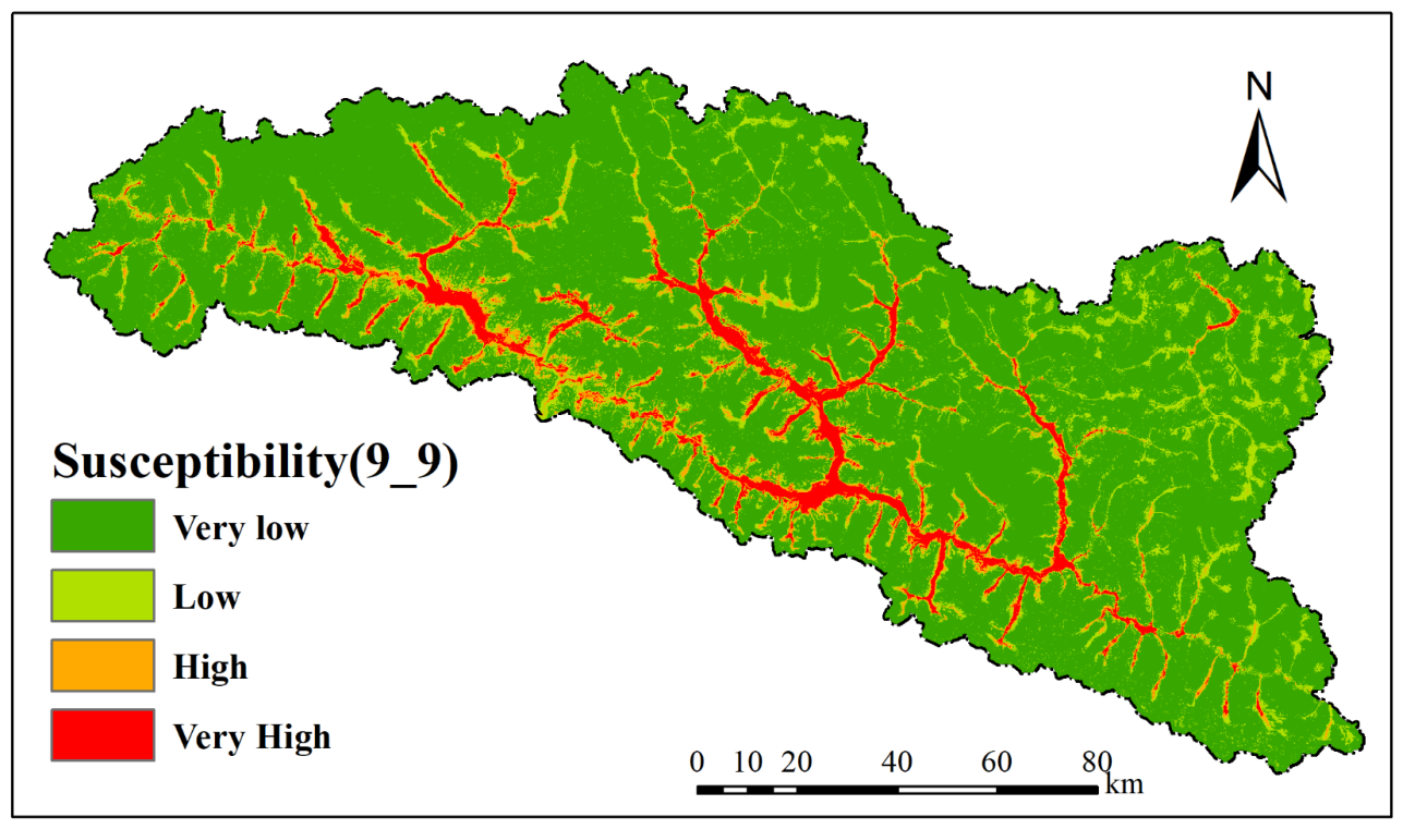
Figure 4. Micro-geomorphic within a 3 × 3 window.
Applsci 16 08585 g004
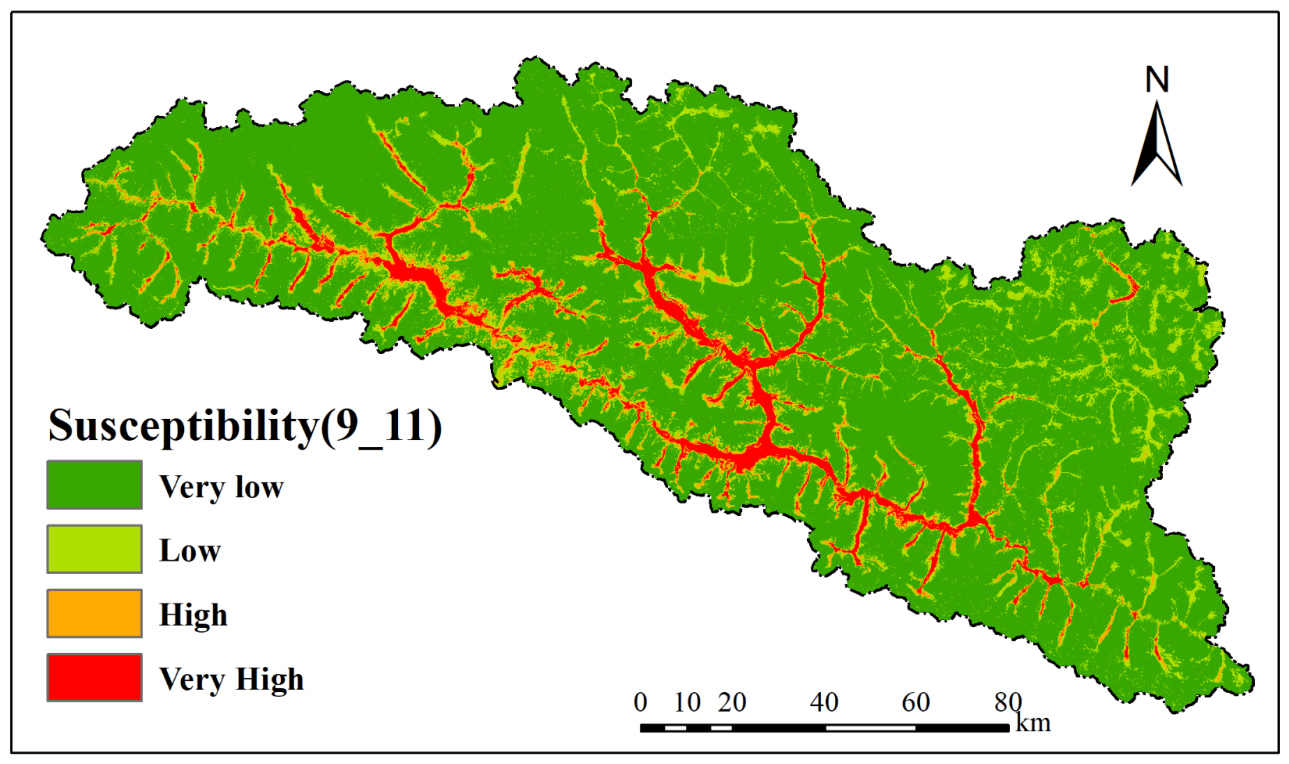
Figure 5. Scale-dependent spatial patterns of micro-geomorphic assemblages ( 5 × 5 to 13 × 13 pixel windows). Columns represent neighborhood frequencies for five process domains. The distinct categories of Fan, Flat, Hillslope, Steep, and Valley are represented by the numerical symbols 1 through 5, respectively.
Applsci 16 08585 g005
Figure 6. Geo-environmental indicators. (a) Drainage line density. (b) Fault line density. (c) Lithology. (d) Vegetation cover.
Applsci 16 08585 g006
Figure 7. OOB feature importance across baseline and multi-scale RF model configurations. Comparison of Δ Error metrics for geo-environmental conditioning variables under baseline, 11 × 11 , and 13 × 13 pixel spatial windows.
Applsci 16 08585 g007
Figure 8. Performance heatmaps evaluating 25 spatial scale combinations across multiple metrics. (a) Accuracy; (b) AUC; (c) F1 Score; (d) Precision; (e) Recall. Y -axes: micro-geomorphic construction windows ( 3 × 3 11 × 11 pixels). X -axes: neighborhood statistical windows ( 5 × 5 13 × 13 pixels). Red boxes indicate optimal performance values.
Applsci 16 08585 g008aApplsci 16 08585 g008b
Figure 9. Multi-scale sensitivity matrix for debris flow susceptibility mapping across nine window combinations. The detailed susceptibility maps (25 figures in total) are presented in Appendix A (Figure A1, Figure A2, Figure A3, Figure A4, Figure A5, Figure A6, Figure A7, Figure A8, Figure A9, Figure A10, Figure A11, Figure A12, Figure A13, Figure A14, Figure A15, Figure A16, Figure A17, Figure A18, Figure A19, Figure A20, Figure A21, Figure A22, Figure A23, Figure A24 and Figure A25). X -axes: neighborhood statistical windows ( 5 × 5 , 9 × 9 , 13 × 13 pixels). Y -axes: localized geomorphological construction windows ( 3 × 3 , 7 × 7 , 11 × 11 pixels).
Applsci 16 08585 g009
Figure 10. Spatial area allocation and debris flow event distribution across susceptibility classes (11 × 11 and 13 × 13 window configurations). Primary axis (bars): area percentage per class. Secondary axis (line): captured historical event percentage.
Applsci 16 08585 g010
Figure 11. Susceptibility mapping evolution across multi-scale neighborhood operators. (ae) Spatial maps under a fixed 3 × 3 geomorphological construction window combined with neighborhood statistical windows from 5 × 5 to 13 × 13 pixels. Right insets: enlarged localized views of high-hazard aggregation zones. The white star symbol indicates the location of a specific debris flow geological hazard.
Applsci 16 08585 g011aApplsci 16 08585 g011b
Figure 12. Susceptibility mapping evolution across micro-geomorphic construction windows. (ae) Spatial maps under a fixed 13 × 13 neighborhood statistical window combined with micro-geomorphic construction windows from 3 × 3 to 11 × 11 pixels. Right insets: enlarged localized views of hazard zone distributions. The white star symbol indicates the location of a specific debris flow geological hazard.
Applsci 16 08585 g012aApplsci 16 08585 g012b
Figure 13. Debris flow susceptibility assessment results. (a) Spatial distribution of debris flow susceptibility levels in Bomi County, classified into four categories from Very low to Very high. (b) Receiver Operating Characteristic curve evaluation of the Random Forest model, with an AUC value of 0.9385.
Applsci 16 08585 g013
Figure 14. Baseline OOB feature importance for the traditional RF model. Bars represent Δ Error values across eight baseline geo-environmental conditioning variables, quantifying relative predictive contributions derived from the bagging process.
Applsci 16 08585 g014
Figure 15. Spatial susceptibility mapping and performance metrics for the baseline SVM model. (a) Debris flow susceptibility map categorized into four hazard levels. (b) ROC curve showing an AUC of 0.9040.
Applsci 16 08585 g015
Figure 16. Baseline permutation feature importance for the SVM model. Bars represent accuracy drop values across eight baseline geo-environmental conditioning variables, quantifying relative predictive contributions derived from the permutation process.
Applsci 16 08585 g016
Table 1. Summary of spatial data sources used for debris flow susceptibility mapping.
Data TypeDescription/ResolutionSourceExtracted Variables
DEMASTER GDEM (30 m)United States Geological Survey (USGS)Slope, aspect, curvature, TPI, roughness, local relief, flow accumulation
Geological Map1:200,000 scaleChina Geological Survey (CGS)Lithology, distance to faults, fault density
Remote Sensing ImageryLandsat 8 OLI (30 m)United States Geological Survey (USGS)NDVI (Normalized Difference Vegetation Index)
Hazard Inventory192 historical events (Point data)Field surveys and historical recordsDependent variable (Debris flow presence/absence)
Table 2. Performance sensitivity matrix of the RF model across 25 combinations of spatial scales.
Construction WindowStatistical WindowAUCAccuracy (%)PrecisionSensitivity (Recall)F1-ScoreRMSEMAE
3 × 35 × 50.93981584.61540.6326530.8857140.7380950.28920.2265
3 × 37 × 70.93981587.41260.6976740.8571430.7692310.26910.2124
3 × 39 × 90.93716988.11190.7250.8285710.7733330.26550.2098
3 × 311 × 110.94431282.51750.5892860.9428570.7252750.29850.2341
3 × 313 × 130.93783188.11190.7045450.8857140.784810.26480.2091
5 × 55 × 50.94298983.91610.6153850.9142860.7356320.29210.2281
5 × 57 × 70.94232888.81120.7317070.8571430.7894740.25820.2045
5 × 59 × 90.93796385.31470.640.9142860.7529410.28470.2228
5 × 511 × 110.93783189.51050.750.8571430.80.25460.2014
5 × 513 × 130.93849286.0140.6530610.9142860.7619050.27850.2188
7 × 75 × 50.93703786.71330.6739130.8857140.7654320.27480.2156
7 × 77 × 70.93849286.0140.6530610.9142860.7619050.27850.2188
7 × 79 × 90.94378388.81120.7317070.8571430.7894740.25770.2042
7 × 711 × 110.94021289.51050.750.8571430.80.25380.2008
7 × 713 × 130.93994787.41260.6888890.8857140.7750.26900.2123
9 × 95 × 50.9470983.91610.6153850.9142860.7356320.29110.2274
9 × 97 × 70.94285787.41260.6976740.8571430.7692310.26820.2117
9 × 99 × 90.93492188.81120.7317070.8571430.7894740.26010.2061
9 × 911 × 110.93637688.81120.7317070.8571430.7894740.25970.2058
9 × 913 × 130.94603284.61540.6274510.9142860.7441860.28780.2253
11 × 115 × 50.94470987.41260.7073170.8285710.7631580.26770.2112
11 × 117 × 70.94232887.41260.6976740.8571430.7692310.26840.2118
11 × 119 × 90.93902188.11190.7142860.8571430.7792210.26420.2087
11 × 1111 × 110.94272588.81120.7317070.8571430.7894740.25800.2044
11 × 1113 × 130.94338690.20980.80.80.80.24710.1972
Table 3. Predictive performance comparison between the proposed multi-scale framework and benchmark classification algorithms.
Model ArchitectureAccuracy (%)PrecisionRecall (Sensitivity)
Baseline Traditional RF81.120.65000.7429
Baseline SVM83.220.68420.7429
XGBoost86.010.72220.7429
LightGBM86.710.73530.7143
Proposed Model ( 11 × 11 / 13 × 13 )90.210.80000.8000
Disclaimer/Publisher’s Note: The statements, opinions and data contained in all publications are solely those of the individual author(s) and contributor(s) and not of MDPI and/or the editor(s). MDPI and/or the editor(s) disclaim responsibility for any injury to people or property resulting from any ideas, methods, instructions or products referred to in the content.